Temperature as a third dimension in column-density mapping of dusty astrophysical structures associated with star formation

Abstract

We present PPMAP, a Bayesian procedure that uses images of dust continuum emission at multiple wavelengths to produce resolution-enhanced image cubes of differential column-density as a function of dust temperature and position. PPMAP is based on the generic “point process” formalism, whereby the system of interest (in this case, a dusty astrophysical structure such as a filament or prestellar core) is represented by a collection of points in a suitably defined state space. It can be applied to a variety of observational data, such as Herschel images, provided only that the image intensity is delivered by optically thin dust in thermal equilibrium. PPMAP takes full account of the instrumental point spread functions and does not require all images to be degraded to the same resolution. We present the results of testing using simulated data for a prestellar core and a fractal turbulent cloud, and demonstrate its performance with real data from the Hi-GAL survey. Specifically, we analyse observations of a large filamentary structure in the CMa OB1 giant molecular cloud. Histograms of differential column-density indicate that the warm material ($T\stackrel{{\scriptstyle>}}{{{}_{\sim}}}13$ K) is distributed log-normally, consistent with turbulence, but the column-densities of the cooler material are distributed as a high density tail, consistent with the effects of self-gravity. The results illustrate the potential of PPMAP to aid in distinguishing between different physical components along the line of sight in star-forming clouds, and aid the interpretation of the associated PDFs of column density.

1 Introduction

Observations of thermal dust emission from Galactic structures, such as starless cores, filaments, and bubbles in the interstellar medium (ISM), can provide key information on the initial conditions for star formation. Significant advances in the modelling of these structures have been made possible by the availability of submillimetre imaging data at multiple wavelengths, such as that provided by Herschel (Pilbratt et al., 2010) and various ground-based telescopes. The data carry information on physical parameters such as the density and temperature structure of prestellar cores and their filamentary environments, as well as that of the turbulent medium from which those structures are believed to evolve. The parameter estimation typically involves the fitting of modified blackbody models to the observed spectral energy distributions (SEDs). This may carried out on a pixel-by-pixel basis so as to produce maps of integrated column density and mean line-of-sight dust temperature (sometimes referred to as column temperature).

In the standard procedure (see, for example, Könyves et al., 2010; Peretto et al., 2010; Bernard et al., 2010), the images at all wavelengths are first smoothed to a common spatial resolution which, in the case of Herschel data, means the resolution at the longest wavelength, i.e., 500 $\mu$m. A variant of this technique (Palmeirim et al., 2013) uses spatial filtering to restore (with the possible exception of the cooler structures) the 250 $\mu$m spatial resolution. Three physical assumptions underlying these procedures are: (i) the dust along a given line of sight has uniform temperature, (ii) the ratio of gas to dust is uniform, and (iii) the dust opacity law is constant and represented by a power-law, $\kappa_{\lambda}\propto\lambda^{-\beta}$, as a function of wavelength, $\lambda$, with $\beta$ normally being taken as 2. The latter assumption may be relaxed by allowing $\beta$ to vary (e.g., Gordon et al., 2014), although care must be exercised in order to avoid spurious correlations due to the degeneracy between dust temperature, $T$, and $\beta$ (Kelly et al., 2012; Veneziani et al., 2013).

Since the structures of interest are, in general, not isothermal, assumption (i) is often a poor one. This is particularly true of structures such as prestellar cores, which have large temperature gradients. Those gradients can have significant effects on parameter values estimated from SED fits. For example, Malinen et al. (2011) showed that line-of-sight temperature variations can lead to underestimates in mass. Also, Shetty et al. (2009) found that the temperature variations result in poor fits of the peaks of SEDs to the models, and that temperature estimates based on simple SED fits can provide only upper limits to the coldest temperatures along the line-of-sight.

If observational images are available at several (at least three) wavelengths, there is information contained in the data which allows us to constrain the distribution of temperature on the line of sight. We accomplish this goal by using the set of observed images to produce an image cube consisting of a stack of 2D images of differential column-density, where each image in the stack represents the column-density at a different dust temperature. This is an application of the more generic “point process” algorithm (Richardson & Marsh, 1987, 1992), and we therefore refer to the new procedure as point process mapping, or PPMAP.

2 Mathematical Basis

2.1 Point Processes

A point process is defined as a random set of points in a suitably-defined state space. It provides a conceptual framework for representing an astrophysical system as a collection of primitive “objects”, each of which is characterised by a set of parameters. Those parameters then constitute the axes of a “single-object state space”, so that the system itself is represented by a distribution of points in such a space. In the present context, the system may be a filament, bubble, core, or molecular cloud, and the constituent “objects” are small building blocks, each of unit column-density and uniform temperature. Each such object is then characterised by three parameters: 2D position projected onto the plane of the sky $(x,y)$, and dust temperature $(T)$; it can thus be represented as a point in a three-dimensional state space. We divide the state space into a rectangular grid of $N_{\rm st}$ cells corresponding to the total number of states; the column-density distribution as a function of position and temperature is then defined by the set of occupation numbers of those cells, represented by vector ${\mathbf{\Gamma}}$ which is referred to as the “state” of the system.

2.2 Measurement Model

We assume that the astrophysical structure is optically thin to the radiation emitted by dust at all observed wavelengths. Consequently the images are the superposition of the instrumental responses to all of the individual component objects, whose number is denoted by $N$. Each object is defined to have unit column-density and a spatial profile corresponding to a circular Gaussian whose full width at half maximum corresponds to 2 pixels in the positional grid. The measurement model can then be expressed as:

$${\mathbf{d}}={\mathbf{A}}{\mathbf{\Gamma}}+{\mathbf{\mu}}\,.$$ (1)

Here, ${\mathbf{d}}$ is the measurement vector whose $m^{\rm th}$ component represents the pixel value at location $(X_{m},Y_{m})$ in the observed image at wavelength $\lambda_{m}$; $\;{\mathbf{\mu}}$ is the measurement noise, assumed to be a Gaussian random process with covariance ${\mathbf{C}}_{\mu}$; $\;{\mathbf{A}}$ is the system response matrix whose $mn^{\rm th}$ element expresses the response of the $m^{\rm th}$ measurement to an object which occupies the $n^{\rm th}$ cell in the state space, corresponding to spatial location $(x_{n},y_{n})$ and dust temperature $T_{n}$; it is given by

$$A_{mn}=H\!_{\lambda_{m}}\!(X_{m}\!\!-\!\!x_{n},Y_{m}\!\!-\!\!y_{n})\,K\!_{\lambda_{m}}\!(T_{n})B\!_{\lambda_{m}}\!(T_{n})\,\kappa(\lambda_{m})\,\Delta\Omega_{m}\,.$$ (2)

Here, $H_{\lambda}(x,y)$ is the convolution of the point spread function (PSF) at wavelength $\lambda$ with the profile of an individual object; $K_{\lambda}(T)$ is a possible colour correction to the model fluxes due the finite bandwidth of the observations; $B_{\lambda}(T)$ is the Planck function; $\Delta\Omega_{m}$ is the solid angle subtended by the $m^{\rm th}$ pixel and $\kappa(\lambda)$ is the dust opacity law. We could use any appropriate functional form for the latter, but for present purposes we adopt a simple power law with a constant index of $\beta=2$, i.e.,

$$\kappa(\lambda)=0.1\,{\rm cm}^{2}\,{\rm g}^{-1}\,\left(\frac{\lambda}{300\,\mu{\rm m}}\right)^{-2}\,.$$ (3)

Eq. (3) provides a reasonably good approximation (to within $\sim 50$%) when applied to observations of starless cores (Roy et al., 2014). The reference opacity (0.1 cm² g^-1 at 300 $\mu$m) is defined with respect to total mass (dust plus gas). Although observationally determined, it is consistent with a gas to dust ratio of 100 (Hildebrand, 1983).

The state vector, ${\mathbf{\Gamma}}$, is regarded as another random process; its individual components, $\Gamma_{n}$, are assumed to be statistically independent and binomially distributed a priori, i.e.

$$P(\Gamma_{n})=\begin{cases}\frac{N!}{\Gamma\!_{n}!(N-\Gamma\!_{n})!}\,p^{\Gamma\!_{n}}(1-p)^{N-\Gamma_{n}}&\mbox{if }\Gamma_{n}\in\{0,\ldots,N\},\\ 0,&\mbox{otherwise. }\end{cases}$$ (4)

Here $p$ is the probability that any given cell is occupied when there is only one object present, i.e. $p=1/N_{\rm st}$. The a priori mean of $\Gamma_{n}$ is equal to the constant value $\eta$ for all $n$, where $\eta=N_{0}/N_{\rm st}$ and $N_{0}$ is the a priori expectation number of objects. For sufficiently large $N$ (in practice, $N\stackrel{{\scriptstyle>}}{{{}_{\sim}}}20$), the deMoivre-Laplace theorem enables Eq. (4) to be approximated by a Gaussian, such that:

$$P(\Gamma_{n})=\frac{1}{\sigma\sqrt{2\pi}}\exp\frac{-(\Gamma_{n}-\eta)^{2}}{2\sigma^{2}}$$ (5)

where $\sigma=\sqrt{\eta(1-p)}$.

In either case, the a priori distribution of possible states is given by

$$P({\mathbf{\Gamma}})=\prod_{n=1}^{N_{\rm st}}P(\Gamma_{n}).$$ (6)

2.3 Solution Methodology

The goal of the procedure is to estimate ${\mathbf{\Gamma}}$ given the data, ${\mathbf{d}}$. The estimation is based on minimising the mean square error, so that the optimal estimate is then the a posteriori average value of ${\mathbf{\Gamma}}$, given by:

$$\rho({\mathbf{z}}_{n}|{\mathbf{d}})\equiv E(\Gamma_{n}|{\mathbf{d}})=\sum_{\mathbf{\Gamma}}\Gamma_{n}P({\mathbf{\Gamma}}|{\mathbf{d}})\,.$$ (7)

Here, ${\mathbf{z}}_{n}$ is a 3-dimensional vector representing the coordinates $(x_{n},y_{n},T_{n})$ of the $n^{\rm th}$ cell in state space. The conditional probability, $P({\mathbf{\Gamma}}|{\mathbf{d}})$, is given by Bayes’ rule,

$$P({\mathbf{\Gamma}}|{\mathbf{d}})=\frac{P({\mathbf{d}}|{\mathbf{\Gamma}})\,P({\mathbf{\Gamma}})}{P({\mathbf{d}})}\,,$$ (8)

where $P(\Gamma)$ is given by (6), $P({\mathbf{d}})$ serves as a normalisation factor,

$$\ln P({\mathbf{d}}|{\mathbf{\Gamma}})=-\frac{1}{2}({\mathbf{d}}-{\mathbf{A}}{\mathbf{\Gamma}})^{\rm T}{\mathbf{C}}_{\mu}^{-1}({\mathbf{d}}-{\mathbf{A}}{\mathbf{\Gamma}})+{\rm const.}$$ (9)

and ${\rm T}$ denotes the transpose.

We refer to $\rho({\mathbf{z}}|{\mathbf{d}})$ as a density since it represents the average local density of occupied cells in the state space of position and temperature. Its estimation is a generic problem in statistical mechanics, and its solution has been discussed previously in connection with acoustical imaging (Richardson & Marsh, 1987), target tracking (Richardson & Marsh, 1992), and the detection of planets using interferometric data (Marsh, Velusamy & Ware, 2006). We use a stepwise approach in which we start by artificially increasing the measurement noise to the point at which the measurements contribute essentially no information; the optimal solution is then simply the a priori mean density which is flat everywhere. We then gradually decrease the noise back down to the true value, updating $\rho({\mathbf{z}}|{\mathbf{d}})$ at each step. The process can be regarded as a time sequence of noisy measurements whose cumulative effect is to build the signal to noise ratio (SNR) back up to the correct value. The “time” corresponds to a progress variable, $t$, representing the degree of conditioning on the data, and its value increases from 0 to 1 during the estimation process. On this basis we rewrite our measurement model as

$${\mathbf{d}}(t)={\mathbf{A}}{\mathbf{\Gamma}}(t)+{\mathbf{\nu}}(t)\,,$$ (10)

where ${\mathbf{\nu}}(t)$ represents the artificially increased measurement noise, assumed to be uncorrelated between “time” samples, i.e.

$$E\nu(t)\nu(t^{\prime})^{\rm T}={\mathbf{R}}_{\nu}\delta(t-t^{\prime})\,,$$ (11)

where ${\mathbf{R}}_{\nu}$ is an appropriately scaled version of ${\mathbf{C}}_{\nu}$.

The solution procedure is obtained from a hierarchy of integro-differential equations involving densities of all orders. Fortunately, the hierarchy can be truncated, to good approximation, at the first member. We then obtain

$$\frac{\partial\rho}{\partial t}+\phi_{1}\rho=0\,,$$ (12)

where $\phi_{1}$ is the conditioning factor, given by

$$\phi_{1}=-\,({\mathbf{d}}-{\mathbf{A}\rho})^{\rm T}{\mathbf{R}_{\nu}}\!\!\!^{-1}{\mathbf{A}}+{\mathbf{b}}/2,$$ (13)

and ${\mathbf{b}}$ represents a vector formed from the diagonal elements of ${\mathbf{A}}^{\rm T}{\mathbf{R}_{\nu}}\!\!\!^{-1}{\mathbf{A}}$.

The optimal ${\mathbf{\rho}}$, denoted $\hat{\mathbf{\rho}}$, is obtained by numerically integrating Eq. (12) from $t=0$ to $t=1$ in steps of size $\delta t$, chosen to be small enough that the integrand changes approximately linearly between steps; the initial condition is $\rho_{(t=0)}=\eta$. The desired image cube of differential column-density is then obtained by mapping the set of $\hat{\rho}_{n}$ back onto the 3D grid of coordinates $(x_{n},y_{n},T_{n})$.

We refer to the quantity $\eta$ as the a priori dilution; it represents the degree to which the procedure is forced to represent the data with the least number of objects. In principle, $\eta$ should be set at the smallest value for which the reduced chi squared, $\chi_{\nu}^{2}$, is of order unity, where:

$$\chi_{\nu}^{2}=\frac{1}{M}\sum_{i}\frac{({\mathbf{d}}-{\mathbf{A}\hat{\rho}})_{i}^{2}}{(C_{\mu})_{ii}},$$ (14)

and $M$ is the number of measurements, i.e. the total number of pixels at all wavelengths. In practice, values in the range 0.1–0.01 typically suffice. Provided $\eta$ (or equivalently, $N_{0}$) has been appropriately chosen, the final number of representative objects (equal to $\sum_{n}{\hat{\rho}_{n}}$) should correspond approximately to $N_{0}$.

Having obtained $\hat{\mathbf{\rho}}$, the corresponding uncertainties may be obtained from the matrix of 2nd derivatives of $\ln P({\mathbf{\rho}}|{\mathbf{d}})$ with respect to the components of ${\mathbf{\rho}}$, using the procedure described by Whalen (1971). Based on the Gaussian approximation of Eq. (5), making use of Eqs. (8) and (9), we construct a matrix, ${\mathbf{\gamma}}$, as follows:

$${\mathbf{\gamma}}={\mathbf{A}}^{\rm T}{\mathbf{C}_{\mu}}^{-1}{\mathbf{A}}\,\,+\,\,\frac{1}{\eta}\,{\mathbf{I}}$$ (15)

where ${\mathbf{I}}$ is the identity matrix of order $N_{\rm st}$. The uncertainties in the $\hat{\rho}_{n}$ values are then given by:

$$\sigma_{\hat{\rho}_{n}}=[(\gamma^{-1})_{nn}]^{\frac{1}{2}}$$ (16)

The uncertainties become larger in localised regions of high source density, where the number of objects required to represent the astrophysical structure greatly exceeds the originally assumed $N_{0}$. In such regions a better approximation is provided by replacing $\eta$ in Eq. (15) with its a posteriori value, $\hat{\eta}$, given by:

$$\hat{\eta}=(\sum_{n=1}^{N_{\rm st}}\hat{\rho}_{n})/N_{\rm st}$$ (17)

The above approach is motivated by two important considerations:
(i) Direct maximisation of the a posteriori probability would involve searching a prohibitively large parameter space. For example, if we characterise each of $N_{\rm obj}$ objects by $N_{\rm p}$ parameters (which in this case would be $x,y,T,$ and differential column-density), we would need to search an $N_{\rm obj}N_{\rm p}$-dimensional space for the maximum probability (or, equivalently, the minimum of a weighted chi squared function) and this would be computationally intractible for any reasonable model size. By contrast, the procedure described above is guaranteed to reach the globally optimal solution in a limited number of steps without searching a multi-object parameter space.
(ii) The use of an occupation number formalism means that the computational burden does not increase with the number of objects.

3 Tests with synthetic data

3.1 Prestellar core model

Our first test of PPMAP was based on synthetic data for a $0.8\,{\rm M}_{{}_{\odot}}$ prestellar core, modelled as a critical Bonnor-Ebert sphere with central density $n_{{}_{{\rm H}_{2}}}=1.65\times 10^{5}\,{\rm cm}^{-3}$ and radius $R=0.049\,{\rm pc}$, embedded in a cloud of visual absorption, $A_{V}=1\,{\rm mag}$, and located at a distance of $140\,{\rm pc}$. The radial profile of dust temperature for this model, and the isophotal maps observable with Herschel were computed using the PHAETHON radiative transfer code (Stamatellos & Whitworth, 2003). The model radial profiles of density and temperature are shown in Fig. 1.

Figure 1: Radial profiles in the modelled prestellar core. (a) Relative density, $n_{{\rm H}_{2}}/(1.65\times 10^{5}\,{\rm cm}^{-3})$. (b) Temperature, $T[{\rm K}]$.

The model profiles were used to generate synthetic Herschel images at the SPIRE/PACS nominal wavelengths of $\lambda[\mu{\rm m}]=70,\,160,\,250,\,350\;{\rm and}\;500$, by calculating the intensity distribution on the plane of the sky, using the dust opacity law defined by Eq. (3). These intensity distributions were then convolved with the PACS and SPIRE PSFs for the appropriate wavelength bands (Poglitsch et al., 2010; Griffin et al., 2013) and synthetic Gaussian measurement noise is added, based on an assumed SNR of 300 at all bands. Fig. 2 shows the result for $\lambda=250\,\mu{\rm m}$.

Figure 2: Simulated observational image of the model prestellar core at $\lambda=250\,\mu{\rm m}$. The width of the field of view is $6^{\prime}$, corresponding to $0.24\,{\rm pc}$ at the assumed distance of $140\,{\rm pc}$.

3.1.1 Results obtained using standard procedure

Before processing the synthetic images with PPMAP, we first examine the results obtained by applying the standard procedure. In the latter, all the maps are smoothed to the resolution of the $500\,\mu{\rm m}$ image, each pixel is then allocated a mean temperature on the basis of its SED, and finally this temperature is used to estimate the column-density of each pixel. The results are shown in Fig. 3.

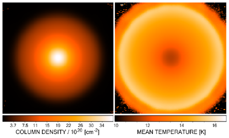
Figure 3: Maps of (a) column-density, and (b) dust temperature, for the model prestellar core, obtained by applying the standard procedure, in which the dust temperature is assumed to be uniform along the line of sight. The field of view is $6^{\prime}\times 6^{\prime}$.

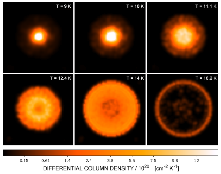
Figure 4: Maps of differential column-density on six temperature planes at $T[{\rm K}]=9.0,\,10.0,\,11.1,\,12.4,\,14.0\;{\rm and}\;16.2$, computed using PPMAP on simulated observations of the model prestellar core. The field of view of each panel is $6^{\prime}\times 6^{\prime}$.

Figure 5: Profiles of differential column-density on lines through the centre of the model prestellar core, for the temperature planes at $T[{\rm K}]=9.0,\,10.0,\,11.1,\,12.4,\,14.0\;{\rm and}\;16.2$. The solid lines are obtained with PPMAP; the dashed lines are the true profiles; and the dotted lines give the 1-$\sigma$ uncertainty levels.

3.1.2 Results obtained using PPMAP

The synthetic images were used as input to PPMAP, to produce estimates of the differential column-density in a stack of ten temperature planes corresponding to the following set of possible dust temperatures: $T[{\rm K}]=7.0,\,8.0,\,9.0,\,10.0,\,11.1,\,12.4,\,14.0,\,16.2,\,19.6\;{\rm and}\;25.0$. The resulting differential column-density maps for the six temperature planes with significant values are shown in Fig. 4. They have been expressed in units of cm^-2 K^-1 by dividing the estimated differential column-density in each temperature plane by the temperature interval itself. Fig. 5 shows a central slice through these images, together with the true (model) profiles for comparison.

From the PPMAP results we estimate that the total mass of the model prestellar core plus the cloud in which it is embedded is $0.87\,{\rm M}_{{}_{\odot}}$, which compares well with the true mass of $0.85\,{\rm M}_{{}_{\odot}}$. Likewise, the PPMAP results give the integrated column-density along the line of sight through the centre of the model prestellar core to be $6.88\times 10^{21}\,{\rm H}_{{}_{2}}\,{\rm cm}^{-2}$, which compares well with the true value of $6.58\times 10^{21}\,{\rm H}_{{}_{2}}\,{\rm cm}^{-2}$. By comparison, the standard procedure (i.e. smoothing all images to the lowest common resolution and assuming constant temperature along each line of sight) gives a peak column-density of $3.74\times 10^{21}\,{\rm H}_{{}_{2}}\,{\rm cm}^{-2}$, i.e. too low by almost a factor of 2.

3.2 Fractal turbulent cloud model

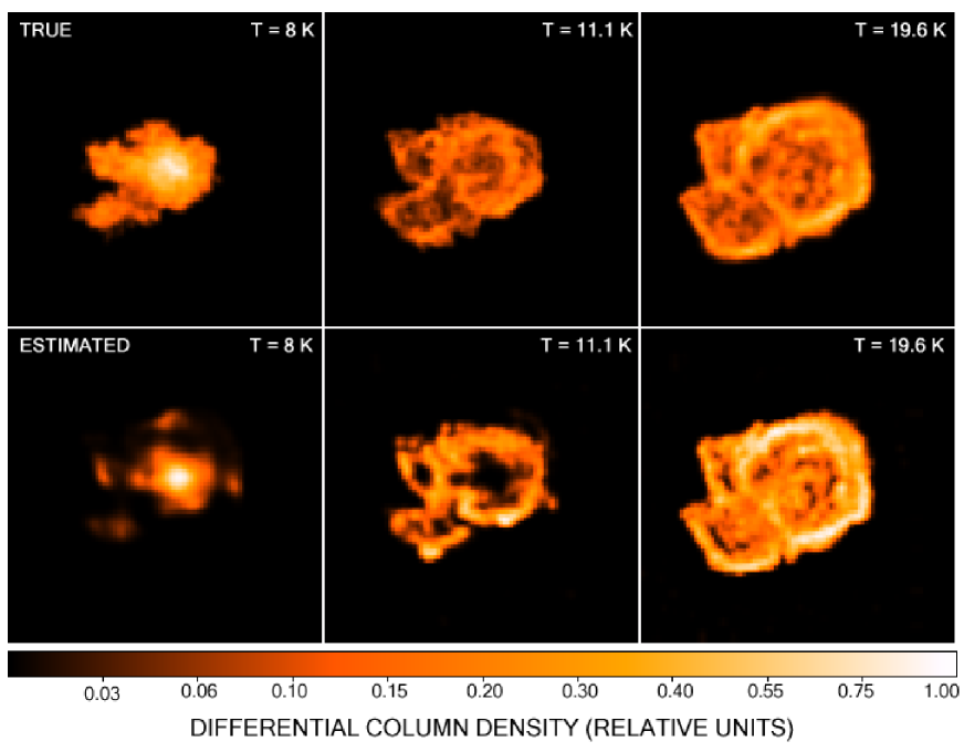
Figure 6: Maps of differential column-density for the fractal turbulent cloud model. The upper row shows the true distributions in three representative temperature intervals centred on 8 K, 11.1 K, and 19.6 K, each with a field of view of $9^{\prime}\times 9^{\prime}$ for an assumed distance of 1 kpc. The lower row shows the inversion results obtained using PPMAP. Within each temperature interval the “true” and “estimated” maps are presented on the same intensity scale, but the map pairs at different temperatures have been normalised to the same peak value of 1.0 in order to bring out the low-level structure. The actual peak values of differential column density, in units of $10^{22}\,{\rm cm}^{-2}{\rm K}^{-1}$, are 6.1, 2.8, and 0.15, at the three temperatures, respectively.

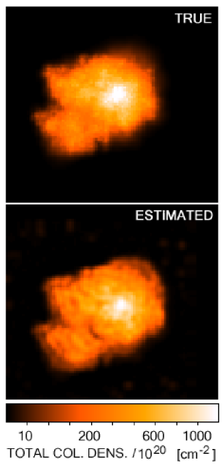
Figure 7: The line-of-sight integrated column density for the fractal turbulent cloud model, with the same field of view as for Fig. 6. The top panel shows the true distribution, and the bottom panel shows the estimated version obtained by summing the differential column density, obtained from PPMAP , over all of the temperature intervals.

We have also tested PPMAP using synthetic data for a model turbulent cloud with fractal structure, i.e., a nested, self-similar hierarchy of clumps within clumps, as described by Walch et al. (2011). We chose a model density distribution with total mass 1000 $M_{\odot}$ and determined its temperature structure via a radiative transfer calculation, assuming it to be bathed in an interstellar radiation field which gives rise to dust temperatures $\sim 7$ K in the centres of clumps and $\sim 20$ K at the cloud periphery. Synthetic Herschel data were generated at the same five wavelengths as above, assuming the structure to be at a distance of 1 kpc. As with the prestellar core model, the emergent intensity distribution was convolved with the Herschel PSFs, and Gaussian noise added (SNR = 300). A set of 2D projections of the assumed 3D model density distribution is shown in the upper portions of Figs. 6 and 7, which represent summations over selected temperature intervals and the total line-of-sight, respectively.

Table 1 presents a summary of the results obtained in the testing of PPMAP on synthetic data for both models, i.e., the prestellar core and fractal turbulent cloud. Wherever possible it includes a comparison with results obtained using the standard techniques for column density mapping. Some conclusions which can be drawn are:

1. For both the prestellar core and fractal cloud, PPMAP yielded peak column densities, total masses and minimum dust temperatures close to the true values, while conventional techniques of column density mapping gave underestimates for peak column density and total mass, and overestimates for the minimum temperature.

2. The apportioning of mass between the different temperature intervals was more accurate in the case of the prestellar core than for the fractal cloud, the median values of fractional error being 15% and 55%, respectively.

Table 1: Results of testing with synthetic data.

				PRESTELLAR CORE						FRACTAL TURBULENT CLOUD
Property	Units			True	PPMAP	Std.	Std.(enhanced)			True	PPMAP	Std.	Std.(enhanced)
$N({\rm H}_{2})_{\rm peak}$	[$10^{21}{\rm cm}^{-2}$]			6.58	6.88	3.74	4.22			125	115	45	47
$T_{\rm min}$	[K]			9.0	9.0	11.9	11.7			7.0	7.0	11.4	13.2
$M(T=7\,{\rm K})$	[$M_{\odot}$]			0.00	0.00	–	–			107	9	–	–
$M(T=8\,{\rm K})$	[$M_{\odot}$]			0.00	0.00	–	–			237	107	–	–
$M(T=9\,{\rm K})$	[$M_{\odot}$]			0.02	0.04	–	–			174	268	–	–
$M(T=10\,{\rm K})$	[$M_{\odot}$]			0.07	0.08	–	–			121	221	–	–
$M(T=11.1\,{\rm K})$	[$M_{\odot}$]			0.13	0.11	–	–			93	130	–	–
$M(T=12.4\,{\rm K})$	[$M_{\odot}$]			0.27	0.24	–	–			79	72	–	–
$M(T=14\,{\rm K})$	[$M_{\odot}$]			0.31	0.37	–	–			70	28	–	–
$M(T=16.2\,{\rm K})$	[$M_{\odot}$]			0.04	0.04	–	–			62	43	–	–
$M(T=19.6\,{\rm K})$	[$M_{\odot}$]			0.00	0.00	–	–			47	73	–	–
$M(T=25\,{\rm K})$	[$M_{\odot}$]			0.00	0.00	–	–			9	4	–	–
$M$(total)	[$M_{\odot}]$			0.85	0.87	0.80	0.81			1000	954	612	612

With regard to item (i), the superior performance of PPMAP can be attributed to the fact that it takes full account of line-of-sight temperature variations. Regarding (ii) it is evident that, for both models, the mass errors for individual temperatures are much larger than the error in total mass, and this reflects the high degree of correlation between the errors. In all cases the mass errors are consistent with the expected uncertainties which, for the fractal cloud are $\sim 85\,M_{\odot}$ at temperatures in the range 7–14 K, decreasing to $4M_{\odot}$ at 25 K. As to the question of why the errors are significantly larger for the fractal cloud than for the prestellar core, the difference probably reflects the information content of the observations relative to the complexity of either model. In particular, Table 1 shows that the prestellar core model has significant mass for only 6 temperatures, whereas the fractal cloud model has significant values for 10 temperatures. The 5 observational wavelengths (in conjunction with prior information) are apparently sufficient to constrain the 6 temperatures of the prestellar core but insufficient to constrain the 10 temperatures of the fractal cloud. In the latter case there is some degeneracy in the tradeoff of differential column density between neighbouring temperatures. When understood in these terms, the difference between the estimated and true values of fractal cloud mass at different temperatures is not as alarming as the 55% error would suggest, since closer inspection shows that the only significant difference is that the peak of the distribution is pushed upwards by $\sim 1$ K. The use of more observational wavelengths would better constrain the distribution.

4 Application to real data

We have applied PPMAP to Herschel data for a region of active star formation in the Galactic plane. The region, part of the CMa OB1 giant molecular cloud, was observed at wavelengths $\lambda[\mu{\rm m}]\simeq 70,\,160,\,250,\,350\;{\rm and}\;500$, as part of the Hi-GAL survey (Molinari et al., 2010), and is described in detail by Elia et al. (2013). We have analysed a $12^{\prime}\!\!.8\times 12^{\prime}\!\!.8$ region centred on $[\ell,b]=[224.\!\!^{\circ}2717,-0.\!\!^{\circ}8361]$, which is dominated by a filamentary ridge at the western periphery of a prominent cavity. Colour corrections were not applied in this inversion, i.e., we assumed $K_{\lambda}(T)=1$. This was because, for the dust temperatures under consideration, the deviations of the correction factors from unity are relatively small over most of the wavelength range ($\stackrel{{\scriptstyle<}}{{{}_{\sim}}}3$% for 160–500 $\mu$m; Sadavoy et al., 2013). Even at 70 $\mu$m, for which the correction is larger, it is still not significant compared to model errors since, in the field under study, essentially all of the 70 $\mu$m emission is due to protostellar point sources which are not well modelled by optically thin dust. Colour corrections would, however, be necessary for other fields in which extended 70 $\mu$m dust emission is present.

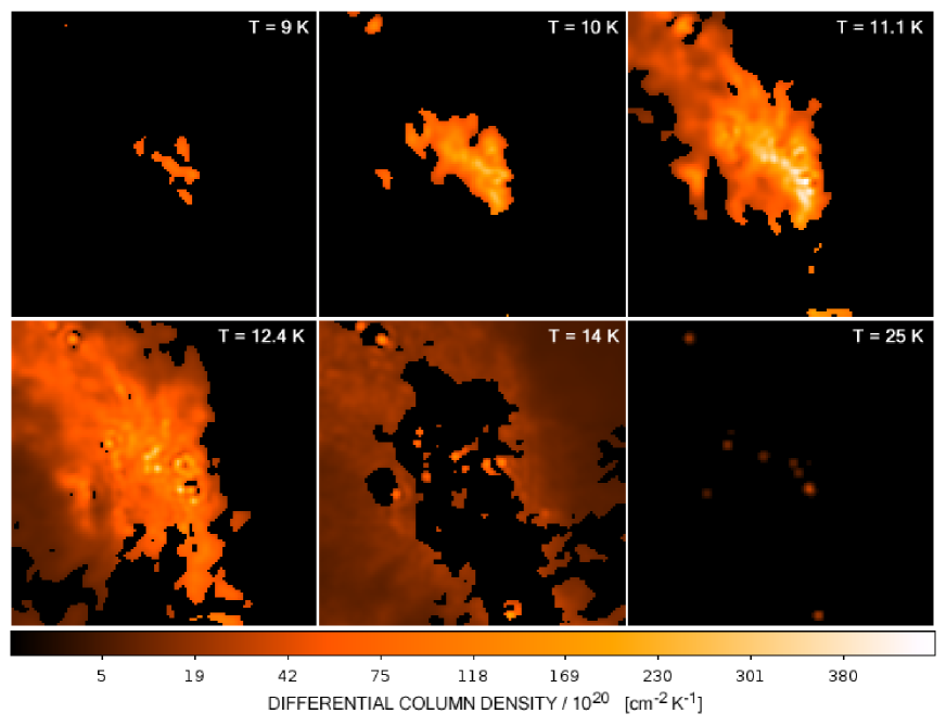
Figure 8: Maps of differential column-density on six representative temperature planes, $T[{\rm K}]=9.0,\,10.0,\,11.1,\,12.4,\,14.1\;{\rm and}\;25.0$, for a filament in the CMa OB1 molecular cloud at $\ell\simeq 224^{\circ}$, observed as part of the Hi-GAL survey. The display scale in each panel has been truncated at the corresponding 1-$\sigma$ uncertainty level. The differential column-densities in the highest temperature panel ($T=25$ K) represent upper bounds when expressed per unit temperature, since the corresponding temperature interval has no upper bound; the displayed values for that particular panel are based on $\Delta T=2.7$ K. The field of view of each panel is $12^{\prime}\!\!.8\times 12^{\prime}\!\!.8$.

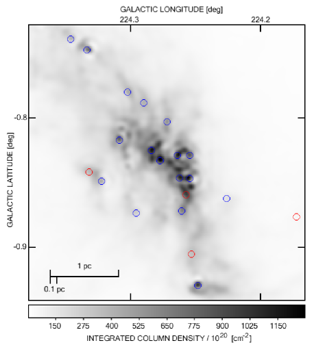
Figure 9: Integrated column-density map of the filamentary complex, obtained by summing the differential column-densities over all temperature planes. The estimated peak column density of hydrogen molecules is $1.35\times 10^{23}\,{\rm cm}^{-2}$. Prestellar and protostellar cores extracted by Elia et al. (2013) are overplotted as red squares and blue circles, respectively. The field of view is the same as for Fig. 8.

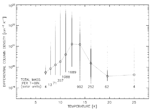
Figure 10: Differential column density as a function of temperature for the filamentary complex. At each discrete temperature, the individual plotted points represent single locations in the 3D space of position and temperature. Open circles represent the median values at each of those temperatures. Below each circle is the total mass of material in the corresponding temperature bin.

Since the computational cost of PPMAP scales approximately as the square of the number of image pixels, we reduced the computation time by analysing the region as a $3\times 3$ mosaic of partially overlapping $6^{\prime}\times 6^{\prime}$ fields. The resulting maps of differential column-density are shown for six representative temperature ranges in Fig. 8; the integrated column-density map, obtained by summing the differential column-density over all temperatures, is shown in Fig. 9. Fig. 10 shows a plot of differential column density as a function of temperature, and includes the total mass at each temperature.

Uncertainties in the differential column density estimates result from a combination of random and systematic effects. The former are due to measurement noise and are well represented by Eq. (16). That equation, however, does not take into account the systematic errors associated with flux calibration. The correlation of those errors between bands could, in principle, result in systematic effects in temperature estimation. However, based on the results of Sadavoy et al. (2013) who simulated such effects for the combination of PACS and SPIRE data, we estimate that the effect of flux calibration errors (including the correlated component) contributes less than 1 K to our temperature uncertainties.

Different structures are visible in the different temperature planes in Fig. 8. These range from dense cores seen at $T[{\rm K}]=9\;{\rm and}\;10$, to protostars seen at $T=25\,{\rm K}$; at the latter temperature, the contribution of the background interstellar medium has disappeared. At the estimated distance of $1.1\,{\rm kpc}$ (Elia et al., 2013), the cores are only marginally resolved and therefore they do not show the shell structure evident in our maps of the model prestellar core (Fig. 4). A shell structure is, however, evident in the filamentary envelope which shows a characteristic depression at $T=14$ K indicative of the lack of interior warm material.

The total mass of the filamentary complex within the analysed $12^{\prime}\!\!.8\times 12^{\prime}\!\!.8$ region, obtained by summing contributions from the pixels of the integrated column-density map of Fig. 9, is $M_{{}_{\rm TOT}}\simeq 4500\,{\rm M}_{{}_{\odot}}$. The mean mass per unit length of the large structure (i.e. the structure filling the frame of Fig. 9) is then $\mu_{{}_{\rm FIL}}\sim 1000\,{\rm M}_{{}_{\odot}}\,{\rm pc}^{-1}$. This is about two orders of magnitude larger than the maximum equilibrium value for an isothermal cylinder at $10\,{\rm K}$, i.e. $\sim\!16\,{\rm M}_{{}_{\odot}}\,{\rm pc}^{-1}$ (Inutsuka & Miyama, 1997), which is consistent with the highly fragmented appearance of the large structure. Many local maxima are visible and the most prominent of these correspond to compact sources extracted by Elia et al. (2013); the locations of the extracted prestellar and protostellar cores are overplotted on Fig. 9.

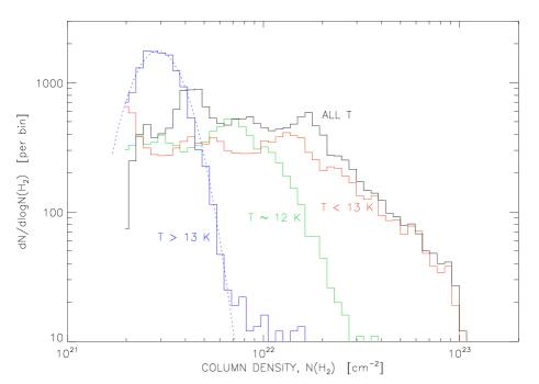
Figure 11: The distribution of column-densities in the filamentary complex. The black histogram represents the distribution of integrated column-density. The red, green, and blue histograms represent the column-densities of material with $T<13$ K, $T\sim 12$ K, and $T>13$ K, respectively. The blue dotted line represents a log-normal function with standard deviation of log column-density equal to 0.28.

The distribution of dust-derived column-density values for the larger ($\sim 9^{\circ}\times 2^{\circ}$) field, which includes the filamentary complex, is presented as a histogram by Elia et al. (2013); it can be characterised as a log-normal distribution with a power-law tail, consistent with the effects of self-gravity on density fluctuations produced by interstellar turbulence (Klessen, 2001; Kainulainen et al., 2009; Kritsuk, Norman & Wagner, 2011; Schneider et al., 2013). The column-density distribution within the $12^{\prime}\!\!.8\times 12^{\prime}\!\!.8$ region under present study is shown by the black histogram in Fig. 11. In contrast to the Elia et al. (2013) plot, no log-normal component is apparent; the most prominent feature is a power-law-like variation at high column densities. However, if instead of considering total column-density we sum the differential column-density over various separate temperature ranges, we obtain a somewhat different picture. This is evident, for example, from the blue and red histograms in Fig. 11, which represent the column-density distributions of the warm ($T>13$ K) and cool ($T<13$ K) material, respectively. Of these, the blue histogram is well fit by a log-normal, whose peak location ($2.9\times 10^{21}\,{\rm cm}^{-2}$) and standard deviation of log column-density (0.28) closely match the log-normal component plotted by Elia et al. (2013)—the latter component, therefore, is still present, even though not apparent in the histogram of integrated column-density for the $12^{\prime}\!\!.8\times 12^{\prime}\!\!.8$ field. The green histogram represents material at $T\sim 12$ K. It appears that the material at this intermediate temperature dominates the flat portion of the total histogram below a column density of $\sim 2\times 10^{22}\,{\rm cm}^{-2}$. It is also the temperature range in which the differential column density reaches its peak, as shown by Fig. 10.

These results might be interpreted to mean that the warm gas (log-normally distributed) has retained the density structure produced by interstellar turbulence while the cool gas has collapsed into cores and comprises the high density tail of the histogram. The reason that the log-normal (turbulent) component is much more prominent in the Elia et al. (2013) histogram is that the latter was derived from a much larger area of sky, over which the total contribution of the warm ISM component was significantly larger than that of the more localised filamentary structure. The material at intermediate temperatures ($\sim 12$ K) may be in a transitional stage of evolution, whereby self gravity has taken over, but the collapse has not yet terminated in a power-law distribution. Such a scenario is consistent with the simulations of Ward, Wadsley & Sills (2014).

We defer a more quantitative analysis of the distribution of differential column density to a forthcoming paper. In that regard we expect that the decomposition of column densities into components at different temperatures will help in resolving some of the issues, currently being debated, in the interpretation of column density PDFs. These include the question of whether the apparent power-law tail can be interpreted more fundamentally as a combination of log-normals (Brunt, 2015), or whether the reverse is true, i.e. that the apparent log-normal components are actually combinations of power-laws with low-column-density turnovers (Lombardi et al., 2015).

5 Discussion

The PPMAP results demonstrate that there is considerably more information in multi-wavelength imaging data than simply the integrated column-density and the mean dust temperature. Even if only the integrated column-density is required, PPMAP provides more accurate estimates of both peak column density and total mass than the standard analysis procedure. The increased accuracy derives both from the ability to capture line-of-sight temperature variations, and from the improved spatial resolution that comes with not having to smooth observational data to the lowest common resolution. The minimum temperature along the line of sight can also be obtained with much greater accuracy, and this is particularly important in the study of starless cores whereby the gas chemistry at core centre is strongly temperature dependent. Moreover, PPMAP-based estimates of column-density and temperature at the centre of a starless core are model- and geometry-independent.

The multi-temperature maps of differential column-density can aid in the interpretation of more complex systems by distinguishing different physical components along the line of sight, as illustrated by our analysis of the filamentary structure in the CMa OB1 cloud. In particular the image cubes served to bring out the log-normal component which was not at all apparent in the distribution of integrated column-density in the immediate vicinity of the filamentary complex. Our future work will include a more quantitative analysis of the functional forms of the PDFs of differential column density at different temperatures. In particular we expect that the temperature decomposition will provide some insight into the issues currently being debated in connection with PDFs of molecular clouds. An additional avenue that we will pursue is to add an additional variable to our state space, namely the index, $\beta$, of the dust opacity law in order to provide information on the spatial variation of grain properties. This will necessitate the inclusion of submillimetre data at longer wavelengths in order to break the well-known degeneracy between temperature and opacity.

Although we have applied the Point Process algorithm to the problem of column density mapping of dusty Galactic structures, the technique itself is far more generic, and can be applied to any system that can be represented as a set of points in a suitably defined parameter space, such that the instrumental response to each point contributes independently to the observations, i.e., the measurement model obeys the superposition principle. In addition the formalism is ideally suited to the study of dynamically evolving systems. To deal with the latter, it is necessary only to add a dynamic term of the form $L\rho$ to Eq. (12), where $L$ is the Fokker-Planck operator (Richardson & Marsh, 1992). This would, for example, provide the ability to integrate on a moving object without knowing, in advance, how fast it is moving or in what direction. The single-object state space would then include not only the $(x,y)$ source position, but two additional variables, $v_{x}$ and $v_{y}$, representing the components of source velocity. One important application might be the detection of near-Earth asteroids, whereby PPMAP has the potential to provide a significant increase in sensitivity.

6 Conclusions

PPMAP is an algorithm designed to produce image cubes of differential column density as a function of angular position and dust temperature for dusty astrophysical structures associated with star formation. The input data consist of a set of observational images at various wavelengths and the associated PSFs. All observational images are used at their native resolution and no smoothing is required.

The performance has been evaluated using simulated Herschel data at five wavelengths between 70 $\mu$m and 500 $\mu$m. Two representative cases were chosen, namely a model prestellar core (embedded Bonnor-Ebert sphere) and a spatially complex model of a fractal turbulent cloud, the dust temperatures being based on a radiative transfer model. In both cases the spatial structure at different temperatures was recovered well. The apportioning of mass between different temperatures was accompished accurately for the prestellar core and reasonably well for the fractal cloud, except for a displacement in the distribution of estimated differential column density by $\sim 1$ K in the latter case. The displacement reflects a limitation in the number of temperatures which can be constrained using observational data at five wavelengths. The temperature resolution can be expected improve with the use of additional observational wavelengths. Comparison with column density maps produced by conventional techniques shows that PPMAP can produce significantly more accurate estimates of peak column density, total mass, and minimum dust temperature within the particular structure.

Application of PPMAP to a filamentary complex observed during the Hi-GAL survey shows that the decomposition into different temperatures facilitates the separation of different physical components along the line of sight and has the potential to provide insight into the mechanisms associated with column density PDFs of molecular clouds.

References

- Bernard et al. (2010) Bernard, J.-Ph., Paradis, D., Marshall, D. J. et al. 2010, A&A, 518, L88
- Brunt (2015) Brunt, C. M. 2015, MNRAS, 449, 4465
- Elia et al. (2013) Elia, D., Molinari, S., Fukui, Y. et al. 2013, ApJ, 772, 45
- Gordon et al. (2014) Gordon, K. D., Roman-Duval, J., Bot, C. et al. 2014, ApJ, 797, 85
- Griffin et al. (2013) Griffin, M. J., North, C. E., Amaral-Rogers, A. et al. 2013, MNRAS, 434, 992
- Hacar et al. (2013) Hacar, A., Tafalla, M., Kauffmann, J, & Kov’acs, A. 2013, A&A 554, 55
- Hildebrand (1983) Hildebrand, R. H. 1983, QJRAS, 24, 267
- Inutsuka & Miyama (1997) Inutsuka, S. & Miyama, S. M. 1997, ApJ, 480, 6811
- Kainulainen et al. (2009) Kainulainen, J., Beuther, H., Henning, T. & Plume, R. 2009, A&A, 508, L35
- Kelly et al. (2012) Kelly, B. C., Shetty, R., Stutz, A. M. et al. 2012, ApJ, 752, 55
- Klessen (2001) Klessen, R. S. 2001, ApJ, 556, 837
- Lombardi et al. (2015) Lombardi, M., Alves, J., & Lada, C. J. 2015, A&A, 576, L1
- Malinen et al. (2011) Malinen, J., Juvela, M., Collins, D. C. et al. 2011, A&A 530, A101
- Könyves et al. (2010) Könyves, V., André, Ph., Men’shchikov, A. et al. 2010, A&A, 518, L106
- Kritsuk, Norman & Wagner (2011) Kritsuk, A. G., Norman, M. L. & Wagner, R. 2011, ApJ, 727, L20
- Marsh, Velusamy & Ware (2006) Marsh, K. A., Velusamy, T. & Ware, B. 2006, AJ, 132, 1789
- Molinari et al. (2010) Molinari, S., Swinyard, B., Bally, J., et al. 2010, PASP, 122, 314
- Palmeirim et al. (2013) Palmeirim, P., André, Ph., Kirk, J. et al. 2013, A&A, 550, A38
- Peretto et al. (2010) Peretto, N., Fuller, G. A., Plume, R. et al. 2010, A&A, 518, 98
- Pilbratt et al. (2010) Pilbratt, G. L., Riedinger, J. R., Passvogel, T., et al. 2010, A&A, 518, L1
- Poglitsch et al. (2010) Poglitsch, A., Waelkens, C., Geis, N., et al. 2010, A&A, 518, L2
- Richardson & Marsh (1987) Richardson, J. M. & Marsh, K. A. 1987, Acoustical Imaging, 16, 615
- Richardson & Marsh (1992) Richardson, J. M. & Marsh, K. A. 1992, in Maximum Entropy and Bayesian Methods, ed. C. R. Smith et al. (Dordrecht: Kluwer), 213
- Roy et al. (2014) Roy, A., André, Ph., Palmeirim, P. et al. 2014, A&A, 562, A138
- Sadavoy et al. (2013) Sadavoy, S. I., Di Francesco, J., Jonhstone, D. 2013, ApJ, 767, 126
- Schneider et al. (2013) Schneider, N., André, Ph., Könyves, V. et al. 2013, ApJ, 766, L17
- Shetty et al. (2009) Shetty, R., Kauffmann, J., Schnee, S. et al. 2009, ApJ, 696, 2234
- Stamatellos & Whitworth (2003) Stamatellos, D. & Whitworth, A. P. 2003, A&A, 407, 941
- Veneziani et al. (2013) Veneziani, M., Piacentini, F., Noriega-Crespo, A. et al. 2013, ApJ, 772, 56
- Walch et al. (2011) Walch, S., Whitworth, A., Bisbas, T. et al. 2011, in Computational Star Formation, Proc. IAU Symp. No. 270, 323
- Ward, Wadsley & Sills (2014) Ward, R. L., Wadsley, J. & Sills, A. 2014, MNRAS, 445, 1575
- Whalen (1971) Whalen, A. D., “Detection of Signals in Noise” (New York: Academic Press)