Abstract Interpretation with Higher-Dimensional Ellipsoids
and Conic Extrapolation

Abstract

The inference and the verification of numerical relationships among variables of a program is one of the main goals of static analysis. In this paper, we propose an Abstract Interpretation framework based on higher-dimensional ellipsoids to automatically discover symbolic quadratic invariants within loops, using loop counters as implicit parameters. In order to obtain non-trivial invariants, the diameter of the set of values taken by the numerical variables of the program has to evolve (sub-)linearly during loop iterations. These invariants are called ellipsoidal cones and can be seen as an extension of constructs used in the static analysis of digital filters. Semidefinite programming is used to both compute the numerical results of the domain operations and provide proofs (witnesses) of their correctness.

keywords: static analysis, semidefinite programming, ellipsoids, conic extrapolation

1 Introduction

Ellipsoids have been widely used to overapproximate convex sets. For instance, in Control Theory they naturally arise as sublevel sets of quadratic Lyapunov functions. They are chosen to minimize some criterion, such as the volume. In Abstract Interpretation [9], they have been used to compute bounds on the output of linear digital filters [4, 5]. Roux et al. [6, 7] further extended that approach by borrowing techniques from Semidefinite Programming (SDP). However, all those works try to recover an ellipsoid that is known to exist as the Lyapunov invariant of some control system from the numerical algorithm implementing that system. The analysis algorithms are tailored for the particular type of numerical code considered. Ellipsoids are interesting in and of themselves because they provide a space-efficient yet expressive representation of convex sets in higher dimensions (quadratic compared to exponential for polyhedra). In this paper, we devise an Abstract Interpretation framework [10] to automatically compute an overapproximation of the values of the numerical variables in a program by an ellipsoid.

We focus our attention on the case when the program variables grow linearly with respect to the enclosing loop counters. We call this approximation an ‘ellipsoidal cone’. Our work also relates to the gauge domain [8], which discovers simple linear relations between loop counters and the numerical variables of a program. Even though the definitions of the abstract operations are general, this model arises more naturally when the analyzed system naturally tends to exhibit quadratic invariants, for instance in the analysis of switched linear systems. Section 2 defines the basic ellipsoidal operations and their verification, and Sect. 4 extends this to the conic extrapolation. The soundness of our analysis relies on the verification of Linear Matrix Inequalities (LMI), which we describe in Sect. 3 before delving into the description of ellipsoidal cones. Finally Sect. 5 presents experiments and discusses applications to switched linear systems.

2 Ellipsoidal Operations

Ellipsoids are the building blocks of our conic extrapolation. We define how to compute the result of basic operations (union, affine transformation…). Since there is generally no minimal ellipsoid in the sense of inclusion, we choose the heuristic of minimizing the volume. Other choices, such as minimizing the so called ‘condition number’ or preserving the shape, are compared in [6].

We mainly rely on SDP optimization methods [3, 11, 12] both to find a covering ellipsoid and test the soundness of our result. However, we do not rely on the correctness of the SDP solver. For each operation whose arguments and results are expressed in function of matrices $(A_{i})_{1\leq i\leq r}$, we define a linear matrix inequality (LMI) of the form $\sum\limits_{i=0}^{r}\alpha_{i}A_{i}\succeq 0$, where $A\succeq 0$ means “$A$ is semidefinite positive”, such that proving the soundness of the result is equivalent to showing that the LMI is satisfied for some reals $(\alpha_{i})$. We find $(\alpha_{i})$ candidates using an SDP solver and then verify the inequality with a sound procedure described in Sect. 3.

Definition 1 (Ellipsoid).

$\operatorname{Ell}(Q,c)=\{x\in\mathbb{R}^{n}|(x-c)^{T}Q(x-c)\leq 1\}$ is the definition of an ellipsoid where $c\in\mathbb{R}^{n}$ and $Q$ is a definite positive $n\times n$ matrix. For practical use, we also define the function $F:(Q,c)\mapsto\begin{pmatrix}Q&-Qc\\ -c^{T}Q&~{}c^{T}Qc-1\end{pmatrix}$.

2.1 A Test of Inclusion

Let $\operatorname{Ell}(Q,c)$ and $\operatorname{Ell}(Q^{*},c^{*})$ be two ellipsoids, using the function $F$ of Definition 1 we have the following duality result (proven in [1]):

Theorem 1.

$$\max_{x\in\operatorname{Ell}(Q,c)}\left((x-c^{*})^{T}Q^{*}(x-c^{*})-1\right)=\\ \min_{\lambda,\beta\in\mathbb{R}}\left\{\beta\text{ s.t. }\lambda\geq 0\mbox{ and }\beta E_{n+1}+\lambda F(Q,c)\succeq F(Q^{*},c^{*})\right\}$$

Where $E_{n+1}$ is an $(n+1)\times(n+1)$ matrix, with $(E_{n+1})_{i,j}=1$ if $i=j=n+1$, else $(E_{n+1})_{i,j}=0$. Hence $\operatorname{Ell}(Q,c)\subset\operatorname{Ell}(Q^{*},c^{*})$ if and only if the minimizing value $\beta^{*}$ is nonpositive.

For given $\operatorname{Ell}(Q,c)$, $\operatorname{Ell}(Q^{*},c^{*})$ and candidates $\lambda$ and $\beta$ computed by the SDP solver, the right hand term provides the LMI to check.

2.2 Computation of the Union

Let $(\operatorname{Ell}(Q_{i},c_{i}))_{1\leq i\leq p}$ be $p$ ellipsoids, we want to find an ellipsoid $\operatorname{Ell}(Q^{*},c^{*})$ which is of nearly minimal volume containing them. To do so, we can solve the following SDP problem. It is decomposed into a first part ensuring the inclusion, proven in [1], and a second part describing the volume minimization criterion, proven in [3, example 18d].

The unknowns of the SDP problem are $X$ an $n\times n$ symmetric matrix, $z\in\mathbb{R}^{n}$ a vector, $\Delta$ a lower triangular matrix and real numbers $t$, $(\tau_{i})_{1\leq i\leq p}$ $(u_{i})_{1\leq i\leq 2^{l+1}-2}$ where $n\leq 2^{l}<2n$:

maximize $$t\mbox{ {such that}}$$ (1)

Inclusion conditions, see [1]:

$$\forall i,1\leq i\leq p,\mbox{ }\exists\tau_{i}\geq 0\text{ s.t. }$$

$$\tau_{i}\begin{pmatrix}Q_{i}&~{}-Q_{i}c_{i}&0\\ -c_{i}^{T}Q_{i}&~{}c_{i}^{T}Q_{i}c_{i}-1~{}~{}&0\\ 0&0&0\end{pmatrix}\succeq\begin{pmatrix}X&-z&0\\ -z^{T}~{}&-1~{}&z^{T}\\ 0&z&-X\end{pmatrix}$$

Volume minimization, see [3, example 18d]:

$$\begin{pmatrix}X&\Delta\\ \Delta^{T}&D(\Delta)\end{pmatrix}\succeq 0$$

where $$D(\Delta) \Delta$$ is the diagonal matrix with the diagonal of .

$$\begin{pmatrix}u_{1}&t\\ t&u_{2}\end{pmatrix}\succeq 0\mbox{ and }\forall i,1\leq i\leq 2^{l}-2,\begin{pmatrix}u_{2i+1}&u_{i}\\ u_{i}&u_{2i+2}\end{pmatrix}\succeq 0$$

$$\forall i,2^{l}-1\leq i<2^{l}-1+n,u_{i}=\delta_{i-2^{l}+2}$$

where $$(\delta_{1},\ldots,\delta_{n}) \Delta$$ are the diagonal coefficients of .

$$\forall i,2^{l}-1+n\leq i\leq 2^{l+1}-2,u_{i}=1\mbox{ }$$

We then define $Q^{*}=X$ and $c^{*}=Q^{*-1}z$ (in floating-point numbers, then we possibly increase the ratio of $Q$ to ensure the inclusion condition). We can check that the resulting ellipsoid really contains the others with Theorem 1.

2.3 Affine Assignments

In this section, we are interested in computing the sound counterpart of an assignment $x\leftarrow Ax+b$, where $x$ is the vector of variables, $A$ is a matrix and $b$ a vector.

2.3.1 Computation.

We want to find a minimal volume ellipsoid such that the inclusion  $\operatorname{Ell}(Q^{*},c^{*})\supset\{Ax+b|(x-c)^{T}Q(x-c)\leq 1\}$ is verified.

By a symmetry argument, we can set $c^{*}=Ac+b$. By expanding the inclusion equation, we find   $\{Ax+b|x\in\operatorname{Ell}(Q,c)\}\subset\operatorname{Ell}(Q^{*},Ac+b)\iff Q\succeq A^{T}Q^{*}A$.

Hence $Q^{*}$ is a solution of the following SDP problem with unknowns $X$ an $n\times n$ symmetric matrix, $z\in\mathbb{R}^{n}$ a vector, $\Delta$ a lower triangular matrix and real numbers $t$, $(\tau_{i})_{1\leq i\leq p}$ $(u_{i})_{1\leq i\leq 2^{l+1}-2}$ where $n\leq 2^{l}<2n$:

Volume minimization: (2)

The same constraints and objective as in (1).

Inclusion conditions:

$$Q\succeq A^{T}XA\mbox{ and }\frac{1}{\epsilon}\operatorname{Id}\succeq X\mbox{ where $\operatorname{Id}$ is the $n\times n$ identity matrix and $\epsilon>0$}$$

We then set $Q^{*}=X$ and $c^{*}=Ac+b$.

The second inclusion condition is here to ensure the numerical convergence of the SDP solving algorithm: if $A$ is singular, the image by $A$ of an ellipsoid is a flat ellipsoid. With this condition, we ensure that $\operatorname{Ell}(Q^{*},c^{*})$ contains a ball of radius $\epsilon$.

To add an input defined by the convex hull of a finite set of vectors (for instance a hypercube), we can just compute the sum for every one of these vectors and compute the union [6].

2.3.2 Verification.

The previous procedure gives us inequalities whose correctness ensures that the ellipsoid $\operatorname{Ell}(Q^{*},Ac+b)$ contains the image of $\operatorname{Ell}(Q,c)$ by $x\mapsto Ax+b$. However, $c^{*}=Ac+b$ is computed in floating-point arithmetic, hence the soundness does not extend to our actual result $\operatorname{Ell}(Q^{*},c^{*})$. Therefore, we have to devise a test of inclusion for an arbitrary $c^{*}$. Let us compute the resulting center in two steps: we first assume that $b=0$. We have from [1]:

$$\left(\forall x,x\in\operatorname{Ell}(Q,c)\Rightarrow Ax\in\operatorname{Ell}(Q^{*},c^{*})\right)$$ (3)

$$\iff \max_{x\in\operatorname{Ell}(Q,c)}(x^{T}A^{T}Q^{*}Ax-2x^{T}A^{T}Q^{*}c^{*}+c^{*T}Q^{*}c^{*})\leq 1$$

$$\iff \min_{\lambda,\beta\in\mathbb{R}}\left\{\beta|\lambda\geq 0\mbox{ and }\lambda F(Q,c)+\beta E_{n+1}\succeq G\right\}\leq 0$$

$$\mbox{\quad\quad\quad\quad where }G=\begin{pmatrix}A^{T}Q^{*}A&-A^{T}Q^{*}c^{*}\\ (-A^{T}Q^{*}c^{*})^{T}~{}~{}&c^{*T}Q^{*}c^{*}-1\end{pmatrix}$$

We can hence verify the inclusion by finding suitable parameters and verifying the resulting LMI.

We finally have to perform the sound computation of the center translation $(c+b)$. Again, this is computed in floating-point arithmetic and we may have to increase the ratio of $Q$ to ensure the verification of the inclusion condition in interval arithmetics: in the test of Theorem 1, we first compute $(c+b)$ and $F(Q,c+b)$ in floating-point arithmetic (and possibly increase the ratio), and with the LMI we check that it “contains” $F(Q,c+b)$ directly computed in interval arithmetic.

2.4 Variable Packing

It can be useful to analyze groups of variables independently, and merge the results. Given a set of variables $\{x_{1},\ldots,x_{p},x_{p+1},\ldots,x_{p+q}\}$ and an ellipsoidal constraint over these variables $(Q,c)$, we can find an ellipsoidal constraint linking $x_{1},\ldots,x_{p}$ by computing the assignment defined by the matrix $\begin{pmatrix}I_{p}&0\\ 0&0\end{pmatrix}$.

Given two sets of variables $\{x_{1},\ldots,x_{p}\}$ and $\{x_{p+1},\ldots,x_{p+q}\}$ linked respectively by $(Q_{1},c_{1})$ and $(Q_{2},c_{2})$, their product is tightly overapproximated by: $\operatorname{Ell}\left(\begin{pmatrix}\frac{Q_{1}}{2}&0\\ 0&\frac{Q_{2}}{2}\end{pmatrix},\begin{pmatrix}c_{1}\\ c_{2}\end{pmatrix}\right)$.

3 Verifying Linear Matrix Inequalities

We now describe how we check the LMI’s that determine the soundness of our analysis. We use interval arithmetic: the coefficients are intervals of floating-point numbers. Each atomic operation (addition, multiplication…) is overapproximated in the interval domain.

3.1 Cholesky Decomposition

Recall that the SDP solver gives us an inequality of the form $\sum\limits_{i=0}^{r}\alpha_{i}A_{i}\succeq 0$, and candidate coefficients $(\alpha_{i})$.

We translate each matrix and coefficient into the interval domain, and sum them up in interval arithmetic so that the soundness of the result does not depend on the floating-point computation of the linear expression.

Then, we compute the Cholesky decomposition of the resulting matrix in interval arithmetic. That is, we decompose [16] the matrix $A$ into $A=LDL^{T}$ where $D$ is an interval diagonal matrix and $L$ a (non interval) lower triangular matrix with ones on the diagonal. Checking that $D$ has only positive coefficients implies that $A$ is definite positive.

3.2 Practical Aspects of the Ellipsoidal Operations

3.2.1 The Precision Issue.

The limitation in the precision of the computations makes us unable to actually test whether a matrix is semidefinite positive: we can only decide when a matrix is definite positive “enough”. For instance, standard libraries fail at deciding that the null matrix $0$ is semidefinite positive.

It means that for all the operations and verifications, we have to perform additional overapproximations in addition to those made by the SDP solver, such as multiplying the ratio of the ellipsoid by a number $(1+\epsilon)$. Moreover, in the verification of LMI’s, it can prove useful to explore the neighborhood $\alpha_{i}\pm\epsilon>0$ of the parameters $(\alpha_{i})$. As Roux and Garoche write in [7]: “Finding a good way to pad equations to get correct results, while still preserving the best accuracy, however remains some kind of black magic.”

3.2.2 Complexity Results.

From the complexity results of Porkolab and Khachiyan, the resolution of an LMI with $m$ terms in dimension $n$ has a complexity of $O(mn^{4})+n^{O(\min(m,n^{2}))}$ [13]. Hence the complexity of the abstract operations is polynomial as a function of the dimension $n$ (i.e., the number of variables), with a degree almost always smaller than 4 (for most operations, $m\leq 4$). The complexity of the Cholesky decomposition can be directly computed and is $O(n^{3})$.

4 Conic Extrapolation

Now that the ellipsoidal operations are well defined, we can describe the construction of the conic extrapolation. The goal is to analyze variable transformations when the ellipsoidal radius evolves (sub-)linearly in the value of the loop counters.

Let us have numerical variables $x=(x_{1},\ldots,x_{n})$ and loop counters $y=(y_{1},\ldots,y_{k})$, we want to control the evolution of $x$ depending on the counters $y$, which are expected to be monotonically increasing.

Inspired by the ellipsoidal constraints, we can use intersections of linear inequalities and a quadratic constraint of the form:

Definition 2 (Conic extrapolation).

Let $q$ be a definite positive quadratic form (that is, there is a matrix $Q\succ 0$ such that $\forall x\in\mathbb{R}^{n}$, $q(x)=x^{T}Qx$), $c\in\mathbb{R}^{n}$, and for $i\in\llbracket 1,k\rrbracket$, $\beta_{i}>0$, $\delta_{i}\in\mathbb{R}^{n}$, $\lambda_{i}\in\mathbb{R}$, and $b_{i}$ a boolean value. We define the ellipsoidal cone:

$$\operatorname{Con}((q,c),(\beta_{i},\delta_{i},\lambda_{i},b_{i})_{1\leq i\leq k})=\\ \{(x,y)\in\mathbb{R}^{n}\times\mathbb{R}^{k}|\forall i\in\llbracket 1,k\rrbracket,y_{i}\geq\lambda_{i}\mbox{ }\land\\ \forall i\in\llbracket 1,k\rrbracket,(b_{i}\lor(y_{i}=\lambda_{i}))\mbox{ }\land\\ q(x-c-\sum\limits_{i=1}^{k}(y_{i}-\lambda_{i})\delta_{i})\leq(\sum\limits_{i=1}^{k}\beta_{i}(y_{i}-\lambda_{i})+1)^{2}\}$$

Let $Q$ be the matrix associated with $q$, $\operatorname{Ell}(Q,c)$ is the ellipsoidal base of the cone. The $\lambda_{i}\in\mathbb{R}$ are the base levels of the cone, that is the minimum values of the loop counters (usually zero). The $\delta_{i}\in\mathbb{R}^{n}$ are the directions toward which the cone is “leaning” (for instance, with a single loop iterating $\operatorname{x\leftarrow x+1}$, we would want $\delta$ to be equal to $1$). The $\beta_{i}\in\mathbb{R}$ determine the slope of the cone in each dimension. The $b_{i}$ are boolean values stating, for each dimension, whether an extrapolation has been made in this dimension. That is, do we consider only the $(x,y)$ with $y_{i}=\lambda_{i}$ (case $b_{i}=\operatorname{False}$) or all those with $y_{i}\geq\lambda_{i}$ and verifying the other conditions (case $b_{i}=\operatorname{True}$).

Figure 1: Example for $p=1,k=1$.

4.1 Conditions of Inclusion

We need to be able to test the inclusion of two cones. The following theorem shows that this inclusion can be reframed as conditions that can be verified with an SDP solver.

Theorem 2.

If we consider two cones $C=\operatorname{Con}((q,c),(\beta_{i},\delta_{i},\lambda_{i},b_{i})_{1\leq i\leq k})$ and $C^{\prime}=\operatorname{Con}((q^{\prime},c^{\prime}),(\beta_{i}^{\prime},\delta_{i}^{\prime},\lambda_{i}^{\prime},b_{i}^{\prime})_{1\leq i\leq k})$, then $C\subset C^{\prime}$ if and only if

$$\left\{\begin{aligned} &(i)\quad\forall i\in\llbracket 1,k\rrbracket,\lambda_{i}^{\prime}\leq\lambda_{i}\mbox{ and }\lambda_{i}>\lambda_{i}^{\prime}\Rightarrow b_{i}^{\prime}\\ &(ii)\quad\operatorname{Ell}(q,c)\subset\operatorname{Ell}\left(\frac{q^{\prime}}{(1+\sum\limits_{i=1}^{k}\beta_{i}^{\prime}(\lambda_{i}-\lambda_{i}^{\prime}))^{2}},c^{\prime}+\sum\limits_{i=1}^{k}(\lambda_{i}-\lambda_{i}^{\prime})\delta_{i}^{\prime}\right)\\ &(iii)\quad\forall i\in\llbracket 1,k\rrbracket,b_{i}\Rightarrow\left(b_{i}^{\prime}\mbox{ and }{\beta_{i}^{\prime}}^{2}\geq\max_{u\in\mathbb{R}^{n},q(u)\leq 1}q^{\prime}(\beta_{i}u+\delta_{i}-\delta_{i}^{\prime})\right)\\ \end{aligned}\right.$$

To prove this theorem, we first consider the case when the two cones have the same base levels. That is, we reduce it to the case when all the $\lambda_{i}$’s are equal to $0$.

Lemma 1.

If we consider two cones $C=\operatorname{Con}((q,c),(\beta_{i},\delta_{i},0,b_{i})_{1\leq i\leq k})$ and $C^{\prime}=\operatorname{Con}((q^{\prime},c^{\prime}),(\beta_{i}^{\prime},\delta_{i}^{\prime},0,b_{i}^{\prime})_{1\leq i\leq k})$, then $C\subset C^{\prime}$ if and only if

$$\left\{\begin{aligned} &(i)\quad\operatorname{Ell}(q,c)\subset\operatorname{Ell}(q^{\prime},c^{\prime})\\ &(ii)\quad\forall i\in\llbracket 1,k\rrbracket,b_{i}\Rightarrow\left(b_{i}^{\prime}\mbox{ and }{\beta_{i}^{\prime}}^{2}\geq\max_{u\in\mathbb{R}^{n},q(u)\leq 1}q^{\prime}(\beta_{i}u+\delta_{i}-\delta_{i}^{\prime})\right)\\ \end{aligned}\right.$$

The proof of these two results is postponed to the end of the section.

4.2 Test of Inclusion

Theorem 2 enables us to build a sound test of inclusion between two cones $C$ and $C^{\prime}$. Condition $(i)$ can be directly tested. We can use the procedure of the previous section to test the ellipsoidal inclusion of condition $(ii)$.

Note that in practice, the test of inclusion will be used (during widening iterations) on cones with the same ellipsoidal base. In these cases, we do not want the overapproximations of the SDP solver to reject the inclusion. Therefore we should directly test whether the bases $(Q,c)$ and the $\lambda_{i}$’s are equal (as numerical values) and answer $\operatorname{True}$ for the test of base inclusion in this case.

To perform a sound test on the subcondition of $(iii)$:

$${\beta_{i}^{\prime}}^{2}\geq\max_{u\in\mathbb{R}^{n},q(u)\leq 1}q^{\prime}(\beta_{i}u+\delta_{i}-\delta_{i}^{\prime})$$

we can compute an overapproximation of $M=\max_{u\in\mathbb{R}^{n},q(u)\leq 1}q^{\prime}(\beta_{i}u+\delta_{i}-\delta_{i}^{\prime})$

From Theorem 1, we know that

$$M=1+\min_{s,t\in\mathbb{R}}\left\{t\mbox{ $|$ }s\geq 0\text{ and }sF(\frac{Q}{\beta_{i}^{2}},0)+tE_{n+1}\succeq F(Q^{\prime},\delta_{i}^{\prime}-\delta_{i})\right\}$$

So for any feasible solution $(s,t)$ of this SDP problem, $1+t$ is a sound overapproximation of $M$.

4.3 Affine Operations on Cones

4.3.1 Counter Increment.

The abstract counterpart of a statement $y_{i}\leftarrow y_{i}+v$ for some value $v$, is the operation $\lambda_{i}\leftarrow\lambda_{i}+v$: after the statement, the constraint is verified for $y_{i}-v$, and making this change in Definition 2 leads to the new value of $\lambda_{i}$. To have a sound result, we can compute the sum in interval arithmetic, and take the lower bound. Note that, in general, the loop counters are integer valued. In that case, the value can be computed exactly.

4.3.2 Affine Transformations.

We want to have a sound counterpart for the affine assignment $x\leftarrow Ax+b$ where $A$ is a matrix and $b$ a vector. Let us fix the values of $(y_{i})_{1\leq i\leq k}$ and note $R=(1+\sum\limits_{i=1}^{k}\beta_{i}(y_{i}-\lambda_{i}))$ and $\hat{c}=c+\sum\limits_{i=1}^{k}(y_{i}-\lambda_{i})\delta_{i}$. Let $Q$
be the matrix of $q$. We first want to find $(Q^{\prime},c^{\prime})\text{ such that we have the inclusion }\\ \{Ax+b|x\in\operatorname{Ell}(\frac{Q}{R^{2}},\hat{c})\}\subset\operatorname{Ell}(\frac{Q^{\prime}}{R^{2}},c^{\prime})$. By symmetry, we can set $c^{\prime}=A\hat{c}+b$. Thus, by doing the same calculations as in Sect.2.3, we have

$$\{Ax+b|x\in\operatorname{Ell}(\frac{Q}{R^{2}},\hat{c})\}\subset\operatorname{Ell}(\frac{Q^{\prime}}{R^{2}},c^{\prime})\iff Q\succeq A^{T}Q^{\prime}A$$

The last condition does not depend on the $y_{i}$’s, so for any quadratic form $q^{\prime}$ whose matrix $Q^{\prime}$ verifies $Q\succeq A^{T}Q^{\prime}A$ (which is an SDP equation, we can add the conditions of volume minimization of (1), and $Q^{\prime}\preceq\frac{1}{\epsilon}I_{n}$ with $\epsilon$ small enough, to ensure numerical convergence), we have

$$\{(Ax,y)|(x,y)\in\operatorname{Con}((q,c),(\beta_{i},\delta_{i},\lambda_{i},b_{i})_{1\leq i\leq k})\}\subset\\ \operatorname{Con}((q^{\prime},Ac),(\beta_{i},A\delta_{i},\lambda_{i},b_{i})_{1\leq i\leq k})$$

As in the case of ellipsoidal assignments, $Ac+b$ and $A\delta_{i}$ are computed in floating-point arithmetic. Hence once they are computed, we have to ensure that the resulting numerical cone contains the formally defined cone, i.e. we need to verify the inclusion of ellipsoidal bases with (3) and the procedure described in Sect.2.3. We also need to verify the conic inclusion, i.e. the fact that $\beta_{i}^{\prime}\geq\beta_{i}+\sqrt{q^{\prime}(A\delta_{i}-\delta_{i}^{\prime})}$, where $\beta_{i}^{\prime}$ and $\delta_{i}^{\prime}$ are the parameters of the resulting cone. So we may have to update the parameters and verify the inequalities in a sound manner.

4.4 Addition and Removal of Counters

When the analyzer enters a new loop, it needs to take into account the previous constraint and add a dependency on the current loop counter $y_{i}$. Moreover, when it exits a loop, it needs to build a new constraint overapproximating the previous one that does not involve the counter $y_{i}$.

Ellipsoidal constraints can be seen as conic constraints with $k=0$. Hence we study the problem of adding and removing counters to a conic constraint $\operatorname{Con}((q,c),(\beta_{i},\delta_{i},\lambda_{i},b_{i})_{1\leq i\leq k})$.

4.4.1 Adding a Counter.

Let $y_{k+1}$ be the counter we want to add. Let $\lambda_{k+1}$ be the minimal value of the counter inferred at this point. We set $\beta_{k+1}=0$, $\delta_{k+1}=0$ and $b_{k+1}=\operatorname{True}$ if the value of $y_{k+1}$ at this point of the analysis is not known precisely, else if we know that $y_{k+1}=\lambda_{k+1}$, then $b_{k+1}=\operatorname{False}$.

That gives us the constraint $\operatorname{Con}((q,c),(\beta_{i},\delta_{i},\lambda_{i},b_{i})_{1\leq i\leq k+1})$.

Proof.

It is immediate from Definition 2 and the distinction made on what we know about $y_{i}$, that this constraint overapproximates the set of reachable $(x,y)$ at this point. ∎∎

4.4.2 Removing a Counter.

We now want to remove the counter $y_{k}$ from the conic constraint, provided that we know that $y_{k}\in[\lambda_{k},M]$ with $M<+\infty$ (note that if it happens that $b_{k}=\operatorname{False}$, then $M=\lambda_{k}$).

Figure 2: Removing the counter $y_{k}$, hence projecting along its direction.

Theorem 3.

Let $C=\operatorname{Con}((q,c),(\beta_{i},\delta_{i},\lambda_{i},b_{i})_{1\leq i\leq k+1})$. Then $C$ is convex and we have

$$C_{|y_{k}\in[a,b]}=C\cap\{(x,y)|y_{k}\in[a,b]\}=\operatorname{Conv}(C\cap\{(x,y)|y_{k}=a\lor y_{k}=b\}).$$

where we suppose $a\geq\lambda_{k}$ and where $\operatorname{Conv}(X)$ is the convex hull of $X$.

Proof.

Up to translation, we can assume that $\forall i\in\llbracket 1,k\rrbracket,\lambda_{i}=0$. If $a=b$, it is immediate. We suppose $a<b$. Then, if $Q$ is the matrix of $q$, let $S$ be the inverse of its square root ($S^{-2}=Q$). We have

$$(x,y)\in C\iff q(x-c-\sum\limits_{i=1}^{k}y_{i}\delta_{i})\leq(1+\sum\limits_{i=1}^{k}\beta_{i}y_{i})^{2}$$

$$\iff \exists u\in\mathbb{R}^{p},||u||_{2}\leq 1,x-c-\sum\limits_{i=1}^{k}y_{i}\delta_{i}=(1+\sum\limits_{i=1}^{k}\beta_{i}y_{i})Su$$

$$\iff \exists u\in\mathbb{R}^{p},||u||_{2}\leq 1,x=\frac{y_{k}-a}{b-a}x_{b}+(1-\frac{y_{k}-a}{b-a})x_{a}$$

where $$x_{b}=(c+\sum\limits_{i=1}^{k-1}y_{i}\delta_{i}+(1+\sum\limits_{i=1}^{k-1}\beta_{i}y_{i})Su+b(\delta_{k}+\beta_{k}Su))$$

$$x_{a}=(c+\sum\limits_{i=1}^{k-1}y_{i}\delta_{i}+(1+\sum\limits_{i=1}^{k-1}\beta_{i}y_{i})Su+a(\delta_{k}+\beta_{k}Su))$$

From the previous equivalences, we have $z_{a}=(x_{a},y_{1},\ldots,y_{k-1},a)\in C$ and $z_{b}=(x_{b},y_{1},\ldots,y_{k-1},b)\in C$. Moreover $(x,y)=\frac{y_{k}-a}{b-a}z_{b}+(1-\frac{y_{k}-a}{b-a})z_{a}$. ∎∎

Let $\pi_{y_{k}}$ be the projection along $y_{k}$. Since convexity and barycenters are preserved up to projections, $\pi_{y_{k}}(C_{|y_{k}\in[a,b]})=\operatorname{Conv}(\pi_{y_{k}}(C_{|y_{k}=a})\cup\pi_{y_{k}}(C_{|y_{k}=b}))$. So, by a direct calculation

$$\pi_{y_{k}}(C_{|y_{k}=a}) =\operatorname{Con}((\frac{q}{(1+\beta_{k}(a-\lambda_{k}))^{2}},c+(a-\lambda_{k})\delta_{k}),$$

$$\mbox{\quad\quad\quad\quad\quad\quad\quad\quad}(\frac{\beta_{i}}{1+(a-\lambda_{k})\beta_{k}},\delta_{i},\lambda_{i},b_{i})_{1\leq i\leq k-1})$$

We have a similar equality for $\pi_{y_{k}}(C_{|y_{k}=b})$, hence we just have to compute the join $(\pi_{y_{k}}(C_{|y_{k}=a})\bigsqcup_{\operatorname{Con}}\pi_{y_{k}}(C_{|y_{k}=b}))$, which is an overapproximation of the convex hull of the union.

However, we have to implement this operation such that it is sound when computed in floating-point arithmetic. Via affine transformation, we can soundly compute an ellipsoidal base $\operatorname{Ell}(q^{*},c^{*})$ such that

$$\left\{\begin{aligned} &q(x-(c+(a-\lambda_{k})\delta_{k}))\leq(1+\beta_{k}(a-\lambda_{k}))^{2}\\ &q(x-(c+(b-\lambda_{k})\delta_{k}))\leq(1+\beta_{k}(b-\lambda_{k}))^{2}\\ \end{aligned}\right.\Rightarrow q^{*}(x-c^{*})\leq 1$$

Then, for any $i\in\llbracket 1,k-1\rrbracket$ such that $b_{i}=\operatorname{True}$, if we note $\beta_{i}^{*}$ and $\delta_{i}^{*}$ the parameters of the resulting cone, in order to have an inclusion of $C_{|y_{k}=a}$ and $C_{|y_{k}=b}$ in $C^{*}$, we need to establish by Theorem 2 that:

$$\left\{\begin{aligned} &\beta_{i}^{*2}\geq\max_{\frac{q(u)}{(1+\beta_{k}(a-\lambda_{k}))^{2}}\leq 1}q^{*}(\frac{\beta_{i}}{1+(a-\lambda_{k})\beta_{k}}u+\delta_{i}-\delta_{i}^{*})\\ &\beta_{i}^{*2}\geq\max_{\frac{q(u)}{(1+\beta_{k}(b-\lambda_{k}))^{2}}\leq 1}q^{*}(\frac{\beta_{i}}{1+(b-\lambda_{k})\beta_{k}}u+\delta_{i}-\delta_{i}^{*})\end{aligned}\right.$$

And since from our hypothesis on $\operatorname{Ell}(q^{*},c^{*})$ we know that $q\succeq q^{*}$, we can just set $\delta_{i}^{*}=\delta_{i}$ and the condition becomes $\beta_{i}^{*}\geq\beta_{i}$. So we can just define $\beta_{i}^{*}=\beta_{i}$, hence the resulting cone after the removing of the $k^{\mbox{th}}$ counter is

$$\operatorname{Con}((q^{*},c^{*}),(\beta_{i},\delta_{i},\lambda_{i},b_{i})_{1\leq i\leq k-1})$$

4.5 A Widening Operator

Let $C=\operatorname{Con}((q,c),(\beta_{i},\delta_{i},\lambda_{i},b_{i})_{1\leq i\leq k})$ and $C^{\prime}=\operatorname{Con}((q^{\prime},c^{\prime}),(\beta_{i}^{\prime},\delta_{i}^{\prime},\lambda_{i}^{\prime},b_{i}^{\prime})_{1\leq i\leq k})$. We suppose that $\forall i\in\llbracket 1,k\rrbracket,\lambda_{i}\leq\lambda_{i}^{\prime}$ and $\exists i\in\llbracket 1,k\rrbracket,\lambda_{i}<\lambda_{i}^{\prime}$.

We want to define a widening operator $\bigtriangledown$ over cones. The intuitive idea is that if $C$ “starts strictly below” $C^{\prime}$ (cf. the conditions on the $\lambda_{i}$’s), then $C^{*}=C\bigtriangledown C^{\prime}$ has the same ellipsoidal base as $C$, but its opening has been “widened” to contain $C^{\prime}$. The decision of only changing the opening and the orientation of the cone (i.e., to change only the $\beta_{i}$’s and $\delta_{i}$’s) relies on the hypothesis that the relative shift of $C^{\prime}$ from $C$ has good chances to be reproduced again. Hence the name of “conic extrapolation”.

4.5.1 Definition of $\bigtriangledown_{p}$.

More formally, we first study the special case in which we know that $\operatorname{Ell}(q^{\prime},c^{\prime})\subset C$ and we define a partial widening operator $\bigtriangledown_{p}$.

Let $C^{*}=C\bigtriangledown_{p}C^{\prime}=\operatorname{Con}((q,c),(\beta_{i}^{*},\delta_{i}^{*},\lambda_{i},b_{i}^{*})_{1\leq i\leq k})$. We note $(i),(ii),(iii)$ (resp. $(i^{\prime}),(ii^{\prime}),(iii^{\prime})$) the conditions of Theorem 2 relative to the inclusion $C\subset C^{*}$ (resp. $C^{\prime}\subset C^{*}$). By construction of $C^{*}$, we already have $(ii)$ and with our hypothesis $\operatorname{Ell}(q^{\prime},c^{\prime})\subset C^{\prime}$, we just need to verify $C\subset C^{*}$ to have $(ii^{\prime})$. We can define $\forall i\in\llbracket 1,k\rrbracket,b_{i}^{*}=(b_{i}\lor b_{i}^{\prime}\lor\lambda_{i}<\lambda_{i}^{\prime})$, which gives us $(i)$ and $(i^{\prime})$.

Finally to verify $(iii)$ and $(iii^{\prime})$, we only need to define the $\beta_{i}^{*}$’s and $\delta_{i}^{*}$’s such that

$$\forall i\in\llbracket 1,k\rrbracket,\left\{\begin{aligned} &b_{i}\Rightarrow{\beta_{i}^{*}}^{2}\geq\max_{q(u)\leq 1}q(\beta_{i}u+\delta_{i}-\delta_{i}^{*})\\ &b_{i}^{\prime}\Rightarrow{\beta_{i}^{*}}^{2}\geq\max_{q^{\prime}(u)\leq 1}q(\beta_{i}^{\prime}u+\delta_{i}^{\prime}-\delta_{i}^{*})\\ \end{aligned}\right.$$

which we overapproximate by a triangle inequality for the norm defined by $q$:

$$\forall i\in\llbracket 1,k\rrbracket,\left\{\begin{aligned} &b_{i}\Rightarrow\beta_{i}^{*}\geq\beta_{i}+\sqrt{q(\delta_{i}-\delta_{i}^{*})}\\ &b_{i}^{\prime}\Rightarrow\beta_{i}^{*}\geq\beta_{i}^{\prime}r+\sqrt{q(\delta_{i}^{\prime}-\delta_{i}^{*})}\\ &\quad\quad\quad\mbox{ where }r\geq\min\{\rho>0|\frac{q^{\prime}}{\rho^{2}}\preceq q\}\end{aligned}\right.$$

With the SDP methods of the first section, we can compute an overapproximating $r$. For each $i$, if none of $b_{i}$ or $b_{i}^{\prime}$ is $\operatorname{True}$, then from our hypothesis $\operatorname{Ell}(q^{\prime},c^{\prime})\subset C^{\prime}$, $b_{i}^{*}=\operatorname{False}$ and we do not have to give values to either $\beta_{i}$ or $\delta_{i}$. If only $b_{i}$ (resp. $b_{i}^{\prime}$) is $\operatorname{True}$, then we define $\delta_{i}^{*}=\delta_{i}$ and $\beta_{i}^{*}=\beta_{i}$ (resp. $\delta_{i}^{*}=\delta_{i}^{\prime}$ and $\beta_{i}^{*}\geq r\beta_{i}^{\prime}$).

If $b_{i}=b_{i}^{\prime}=\operatorname{True}$, we want to minimize $\max(\beta_{i}+\sqrt{q(\delta_{i}-\delta_{i}^{*})},\beta_{i}^{\prime}r+\sqrt{q(\delta_{i}^{\prime}-\delta_{i}^{*})}).$ If we fix the $q$-distance $\sqrt{q(\delta_{i}-\delta_{i}^{*})}$, we want to minimize the $q$-distance $\sqrt{q(\delta_{i}^{\prime}-\delta_{i}^{*})}$. With this geometrical point of view, we see that the optimal $\delta_{i}^{*}$ is a barycenter of $\delta_{i}$ and $\delta_{i}^{\prime}$.

So we define $\delta_{i}^{*}=\mu\delta_{i}+(1-\mu)\delta_{i}^{\prime}$ where we want to find $\mu\in[0,1]$ minimizing

$$\max(\beta_{i}+\sqrt{q(\delta_{i}-\mu\delta_{i}-(1-\mu)\delta_{i}^{\prime})},\beta_{i}^{\prime}r+\sqrt{q(\delta_{i}^{\prime}-\mu\delta_{i}-(1-\mu)\delta_{i}^{\prime})})=\\ \max(\beta_{i}+(1-\mu)\sqrt{q(\delta_{i}-\delta_{i}^{\prime})},\beta_{i}^{\prime}r+\mu\sqrt{q(\delta_{i}-\delta_{i}^{\prime})}).$$

Hence, we can exactly (up to floating-point approximations) compute $\mu$, define $\delta_{i}^{*}$ and then $\beta_{i}^{*}$. This construction of $(\beta_{i}^{*},\delta_{i}^{*},b_{i}^{*})_{1\leq i\leq k}$ ensures that $C,C^{\prime}\subset C^{*}$ and defines $\bigtriangledown_{p}$.

4.5.2 Definition of $\bigtriangledown$.

We now study the general case in which the only assumption made is that $\forall i\in\llbracket 1,k\rrbracket,\lambda_{i}\leq\lambda_{i}^{\prime}$ and $\exists i\in\llbracket 1,k\rrbracket,\lambda_{i}<\lambda_{i}^{\prime}$.

We define a cone $C^{+}=\operatorname{Con}((q,c),(\beta_{i}^{+},\delta_{i}^{+},\lambda_{i},b_{i}^{+})_{1\leq i\leq k})$, which contains the ellipsoidal base of the two cones. The definition (with $q$, $c$ and the $\lambda_{i}$) ensures the inclusion of the ellipsoidal base of $C$. Let $R=1+\sum\limits_{i=1}^{k}\beta_{i}^{+}(\lambda_{i}^{\prime}-\lambda_{i})$ and $\Delta=\sum\limits_{i=1}^{k}\delta_{i}^{+}(\lambda_{i}^{\prime}-\lambda_{i})$.

We define $\forall i\in\llbracket 1,k\rrbracket,b_{i}^{+}=(\lambda_{i}<\lambda_{i}^{\prime})$. Let $r=\min\{\rho>0|\frac{q}{\rho^{2}}\preceq q^{\prime}\}$, if we have $\operatorname{Ell}(\frac{q}{r^{2}},c^{\prime})\subset\operatorname{Ell}(\frac{q}{R^{2}},c+\Delta)$ then $\operatorname{Ell}(q^{\prime},c^{\prime})\subset\operatorname{Ell}(\frac{q}{R^{2}},c+\Delta)$ and from the definitions of the $b_{i}^{+}$’s and Definition 2, we would have $\operatorname{Ell}(q^{\prime},c^{\prime})\times\{(\lambda_{1}^{\prime},\ldots,\lambda_{k}^{\prime})\}\subset C^{+}$. To get this result, we need:

$$\operatorname{Ell}(\frac{q}{r^{2}},c^{\prime})\subset\operatorname{Ell}(\frac{q}{R^{2}},c+\Delta)\iff\{q(c^{\prime}-c-\Delta)\leq(R-r)^{2}\}\land\{R\geq r\}$$

If the transformations applied to the cone are affine, the shift can be seen as the difference between centers. So we choose to define $\Delta=c^{\prime}-c$. Then we choose the minimal possible value of $R$ to have a cone as tight as possible: once the $\delta_{i}$’s corresponding to $\Delta$ are computed in floating-point arithmetic, we can define an upper bound on $\sqrt{q(c^{\prime}-c-\Delta)}+r$ and define $R$ accordingly, so that the above inequality is verified.

These definitions of $\Delta$ and $R$ must be implemented in terms of $\beta_{i}^{+}$ and $\delta_{i}^{+}$. Since we ensured that there is at least one $i$ such that $(\lambda_{i}^{\prime}-\lambda_{i})\neq 0$, there is always a solution. If only one $i$ fits this criterion the solution is unique, otherwise a choice must be made on how to weight the different variable.

This uncertainty can be easily explained: recall that in real programs, only one loop counter is increased at a time, so we know what causes the change in our constraint. This is not the case if many loop counters are increased at the same time.

Finally, this definition of $C^{+}$ allows us to define the widening operator $\bigtriangledown$ by: $C\bigtriangledown C^{\prime}=\left(C\bigtriangledown_{p}C^{+}\right)\bigtriangledown_{p}C^{\prime}$. Note that the assumptions of $\bigtriangledown_{p}$ are verified since $C$ and $C^{+}$ have the same ellipsoidal base, and $C^{+}$, hence $C\bigtriangledown_{p}C^{+}$, contains the base of $C^{\prime}$.

To ensure the convergence of the widening sequence in the cases described in Sect. 5, we can use a real widening operator on the $\beta_{i}$’s that sets them to $+\infty$ after a certain number of steps, for instance.

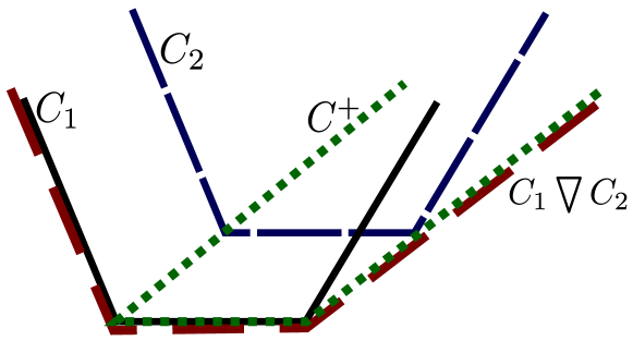
Figure 3: Example showing the various cones involved in the definition of $\bigtriangledown$: $C_{1}$ in black, $C_{2}$ in blue, $C^{+}$ in green and $C_{1}\bigtriangledown C_{2}$ in red.

4.6 Proof of the Characterization of Conic Inclusion

Proof of Lemma 1.

$\bullet$ We first prove that $(i)\land(ii)\Rightarrow C\subset C^{\prime}$. From $(i)$, we know that
$\forall u\in\mathbb{R}^{p},q(u)\leq 1\Rightarrow q^{\prime}(u+c-c^{\prime})\leq 1$. Thus, for $(x,y)\in\mathbb{R}^{p}\times\mathbb{R}_{+}^{k}$ such that $q(x-c-\sum\limits_{i=1}^{k}y_{i}\delta_{i})\leq(1+\sum\limits_{i=1}^{k}\beta_{i}y_{i})^{2}$, we define $\nu=(1+\sum\limits_{i=1}^{k}\beta_{i}y_{i})\geq\sqrt{q(x-c-\sum\limits_{i=1}^{k}y_{i}\delta_{i})}$ and $u=\frac{1}{\nu}(x-c-\sum\limits_{i=1}^{k}y_{i}\delta_{i})$. We have $q(u)\leq 1$.

$$q^{\prime}(x-c^{\prime}-\sum\limits_{i=1}^{k}y_{i}\delta_{i}^{\prime}) =q^{\prime}\left(u+(c-c^{\prime})+(\nu-1)u+\sum\limits_{i=1}^{k}y_{i}(\delta_{i}-\delta_{i}^{\prime})\right)$$ (4)

$$\leq\left(\sqrt{q^{\prime}(u+c-c^{\prime})}+\sum\limits_{i=1}^{k}y_{i}\sqrt{q^{\prime}(\beta_{i}u+\delta_{i}-\delta_{i}^{\prime})}\right)^{2}$$

So if $b_{i}=\operatorname{False}$ then $y_{i}=0$, hence $y_{i}\sqrt{q^{\prime}(\beta_{i}u+\delta_{i}-\delta_{i}^{\prime})}\leq y_{i}\beta_{i}^{\prime}$, and from $(ii)$, if $b_{i}=\operatorname{True}$, then we have the same inequality since $q(u)\leq 1$. So this inequality is true for all $i\in\llbracket 1,k\rrbracket$.

Thus, we have $q^{\prime}(x-c^{\prime}-\sum\limits_{i=1}^{k}y_{i}\delta_{i}^{\prime})\leq(1+\sum\limits_{i=1}^{k}\beta_{i}^{\prime}y_{i})^{2}$ and $\forall i\in\llbracket 1,k\rrbracket$ we have $y_{i}\geq 0$ and from $(ii)$, $y_{i}>0\Rightarrow b_{i}\Rightarrow b_{i}^{\prime}$. So $(x,y)\in C^{\prime}$. So $C\subset C^{\prime}$.

$\bullet$ Now we prove that $C\subset C^{\prime}\Rightarrow(i)\land(ii)$. It is obvious that $C\subset C^{\prime}\Rightarrow(i)$ by taking the intersections of the cones with the set $\{(x,0)\in\mathbb{R}^{p+k}\}$.

If $\exists i\in\llbracket 1,k\rrbracket\text{ s.t. }b_{i}^{\prime}=\operatorname{False}$ and $b_{i}=\operatorname{True}$, then there exist a point $(x,y)$ of $C$ with $y_{i}>0$, so $(x,y)\notin C^{\prime}$ and $C\not\subset C^{\prime}$.

If $\exists i\in\llbracket 1,k\rrbracket\text{ s.t. }b_{i}=\operatorname{True}$ and $\beta_{i}^{\prime}<\max_{q(u)\leq 1}\sqrt{q^{\prime}(\beta_{i}u+\delta_{i}-\delta_{i}^{\prime})}$, then let us take $u\in\mathbb{R}^{p}$ such that $q(u)\leq 1$ and $\beta_{i}^{\prime}<\sqrt{q^{\prime}(\beta_{i}u+\delta_{i}-\delta_{i}^{\prime})}$. We define $x(t)=(1+\beta_{i}t)u+t\delta_{i}+c$.

For any $t\geq 0$, $q^{\prime}(x(t)-c^{\prime}-t\delta_{i}^{\prime})\geq\left(\sqrt{q^{\prime}(u+c-c^{\prime})}-t\sqrt{q^{\prime}(\beta_{i}u+\delta_{i}-\delta_{i}^{\prime})}\right)^{2}\\$

Since $\beta_{i}^{\prime}<\sqrt{q^{\prime}(\beta_{i}u+\delta_{i}-\delta_{i}^{\prime})}$, and from the previous inequality, we have for $t$ big enough, $q^{\prime}(x(t)-t\delta_{i}^{\prime}-c^{\prime})>(1+\beta_{i}^{\prime})^{2}$. By a direct computation $q(x(t)-t\delta_{i}-c)\leq(1+\beta_{i}t)^{2}$. And since $b_{i}=\operatorname{True}$, we have for $y(t)$ such that $y(t)_{i}=t$ and $y(t)_{j\neq i}=0$, $(x(t),y(t))\in C$, $(x(t),y(t))\notin C^{\prime}$ so $C\not\subset C^{\prime}$.

We have proven $\neg(i)\lor\neg(ii)\Rightarrow C\not\subset C^{\prime}$, so we finally have $(i)\land(ii)\iff C\subset C^{\prime}$. ∎∎

Proof of Theorem 2.

Since $(c,(\lambda_{i})_{1\leq i\leq k})\in C$, it is clear that $(i)$ is a necessary condition. Moreover, $C\subset\{(x,y)\in\mathbb{R}^{p+k}|\forall i\in\llbracket 1,k\rrbracket,y_{i}\geq\lambda_{i}\}=:\operatorname{Orth}_{\lambda}$, therefore $C\subset C^{\prime}\iff C\subset C^{\prime}\cap\operatorname{Orth}_{\lambda}\iff C\subset C^{\prime}\cap\operatorname{Orth}_{\lambda}\land(i)$.

Directly from Definition 2, we have for $R=(1+\sum\limits_{i=1}^{k}\beta_{i}^{\prime}(\lambda_{i}-\lambda_{i}^{\prime}))$ the implication $(i)\Rightarrow C^{\prime}\cap\operatorname{Orth}_{\lambda}=\operatorname{Con}((\frac{q^{\prime}}{R^{2}},c^{\prime}+\sum\limits_{i=1}^{k}(\lambda_{i}-\lambda_{i}^{\prime})\delta_{i}^{\prime}),(\frac{\beta_{i}^{\prime}}{R},\delta_{i}^{\prime},\lambda_{i},b_{i}^{\prime})_{1\leq i\leq k})$. So up to translation, we can reduce this case to $\lambda_{i}=\lambda_{i}^{\prime}=0$ and apply Lemma 1.

$$C\subset C^{\prime}\iff C\subset C^{\prime}\cap\operatorname{Orth}_{\lambda}\land(i)$$

$$\iff (i)\land\operatorname{Ell}(q,c)\subset\operatorname{Ell}(\frac{q^{\prime}}{R^{2}},c^{\prime}+\sum\limits_{i=1}^{k}(\lambda_{i}-\lambda_{i}^{\prime})\delta_{i}^{\prime})$$

$$\land\forall i\in\llbracket 1,k\rrbracket,b_{i}\Rightarrow\left(b_{i}^{\prime}\mbox{ and }\frac{{\beta_{i}^{\prime}}^{2}}{R^{2}}\geq\max_{q(u)\leq 1}\frac{q^{\prime}}{R^{2}}(\beta_{i}u+\delta_{i}-\delta_{i}^{\prime})\right)$$

$$\iff (i)\land(ii)\land(iii)$$

∎∎

5 Application and Convergence

1:$x\leftarrow 0\in\mathbb{R}^{n}$

2:for $y$ from 0 to $\infty$ do

3:     pick $i\in\llbracket 1,n\rrbracket$

4:     pick $\epsilon\in\{-1,1\}$

5:     $x_{i}\leftarrow x_{i}+\epsilon$

$n$	2	4	6	8	10	12	14	16
Ell. cones	3s	7s	19s	49s	1m56s	4m16s	8m	12m
Polyhedra	$<$0.1s	$<$0.1s	0.3s	2.5s	54s	47m	$>$1h	$>$1h

Figure 4: Example of a program and its average analysis time on a $2\text{\,}\mathrm{GHz}$ CPU. Ellipsoidal cones have been prototyped in Python using NumPy[17], CVXOPT[15], mpmath[16]. The Apron[18] C library has been used for polyhedra.

In the definition of the conic extrapolation, we did not describe how to choose the ellipsoidal base. For instance, it is possible to get an ellipsoidal shape by computing some iterates of the loop. This seems to work well in the case of programs composed of loops and nondeterministic counter increments: the iterations capture in which direction the counters globally increase (Fig. 2). Since the diameter of the set containing the numerical variables grows linearly, any cone will be overapproximating for $\beta$ big enough.

5.1 Switched Linear Systems

1:$x\leftarrow 0\in\mathbb{R}^{n}$

2:$(A_{i},b_{i})_{1\leq i\leq k}$

3: where $b_{i}\in\mathbb{R}^{n},A_{i}\in\mathcal{M}_{n}(\mathbb{R})$

4:for $y$ from 0 to $\infty$ do

5:     $i\leftarrow\operatorname{rand}(1,n)$

6:     $x\leftarrow A_{i}x+b_{i}$

Benchmark	1	2	3	4	5	6	7
Ell. Cones	1s	2s	2s	2s	1.8s	1.2s	1.3s
Polyhedra	3.2s	16.6s	18s	24s	$>$1h	$>$1h	2m35s

Figure 5: The structure of a Switched Linear System and some benchmarks. Experimental conditions are the same as in Fig. 2. Except for Benchmarks 1 and 2, the resulting polyhedron is trivial.

However, the picture is not as nice if we add linear transformation. This is the case, for instance, for switched linear systems in control theory (Fig.5): if the quadratic form associated with the ellipsoid is not a Lyapunov function of the linear part of the system (of the matrices $A_{i}$ in Fig.5), then the growth of its radius is exponential in the loop counters, and cannot be captured by our conic extrapolation. So if $Q$ is the matrix of the ellipsoidal base of the cone, the Lyapunov conditions should be verified simultaneously : $\forall i,Q-A_{i}^{T}QA_{i}\succeq 0$. This is not always possible, but one can use the SDP solver to try to find a suitable $Q$. Note that the identity matrix is not stable in the sense of control theory and should not be included in the search of $Q$. When $Q$ verifies the Lyapunov conditions, it is easy to show that for $\beta_{i}$ large enough, the cone will be invariant during loops iterations.

5.2 Proof of Convergence with the Lyapunov Condition

Now we show the converse of the assertion of the previous paragraph: if $q$ is a Lyapunov function for the matrix $A$ and $b$ is a vector, then for $\beta$ large enough $C=\operatorname{Con}((q,c),(\beta,\delta,\lambda,\operatorname{True}))$ is stabilized by the iteration of $x\leftarrow Ax+b$.

Proof.

Up to translation, we show the result for $\lambda=0$. We know than for any $x\in C$, $q(x-c-y\delta)\leq(\beta y+1)^{2}$ and by the Lyapunov condition, there exist $\epsilon>0$ such that $\forall x,q(Ax)\leq(1-\epsilon)q(x)$.

Let $\eta=1-\sqrt{1-\epsilon}$ and $M=(A-\operatorname{Id})c+b-\delta$. We have

$$\sqrt{q(Ax+b-c-(y+1)\delta)}=\sqrt{q(A(x-c-y\delta)+(A-\operatorname{Id})(c+y\delta)+b-\delta)}\\ \leq\sqrt{1-\epsilon}(\beta y+1)+\sqrt{q((A-\operatorname{Id})(c+y\delta)+b-\delta)}\\ \leq\beta y+1+\sqrt{q(M+y(A-\operatorname{Id})\delta)}-\eta\beta y\\ \leq\beta y+1+\sqrt{q(M)}+y(\sqrt{q((A-\operatorname{Id})\delta)}-\eta\beta)$$

So for $\beta$ large enough ($\beta>\sqrt{q(M)}$ and $\beta>\sqrt{q((A-\operatorname{Id})\delta)}/\eta$), we have $q(Ax+b-c-(y+1)\delta)\leq(\beta(y+1)+1)^{2}$. ∎∎

6 Concluding Remarks and Perspectives

We proposed an abstract interpretation framework based on ellipsoidal cones to study systems with (sub-)linear growth in loop counters. The aim of this work is twofold: to build an extension of the formal verification of linear systems, and to devise a framework that can be used outside the context of digital filters. Indeed, only the choice of the ellipsoidal base of the cone has to deal with control theory considerations.

The next step is obviously to go beyond the prototype and have a robust implementation to test this framework on actual systems. This will involve a research on how to accurately tune and use the SDP solver, how to deal with precision issues.

The main tools are the SDP solver and the SDP duality to check the soundness of the results of operations via LMI’s. However, we are not bound to use SDP solvers to compute these results, and exploring other options might speed up the analysis.

It would also be interesting to generalize this framework to switched linear systems that are more complex than those studied above. An example is the analysis in [14].

6.0.1 Acknowledgments.

We want to thank Pierre-Loïc Garoche and Léonard Blier for the fruitful conversations we had with each of them during this work, as well as the anonymous referees for the time and efforts taken to review this work.

References

- [1] Yildirim, E. Alper. “On the minimum volume covering ellipsoid of ellipsoids.” SIAM Journal on Optimization 17.3 (2006): 621-641.
- [2] Ros, Lluís, Assumpta Sabater, and Federico Thomas. “An ellipsoidal calculus based on propagation and fusion.” Systems, Man, and Cybernetics, Part B: Cybernetics, IEEE Transactions on 32.4 (2002): 430-442.
- [3] Ben-Tal, A., & Nemirovski, A. (2001). Lectures on modern convex optimization: analysis, algorithms, and engineering applications (Vol. 2). SIAM.
- [4] Feret, J. (2004). “Static Analysis of Digital Filters”. In the 13th European Symposium on Programming-ESOP 2004 (Vol. 2986, pp. 33-48).
- [5] Feret, J. (2005). “Numerical abstract domains for digital filters”. In International workshop on Numerical and Symbolic Abstract Domains (NSAD 2005).
- [6] Roux, P., Jobredeaux, R., Garoche, P. L., Féron, É. (2012). “A generic ellipsoid abstract domain for linear time invariant systems”. In Proceedings of the 15th ACM international conference on Hybrid Systems: Computation and Control (pp. 105-114). ACM.
- [7] Roux, Pierre, and Pierre-Loïc Garoche. “Computing quadratic invariants with min-and max-policy iterations: a practical comparison.” FM 2014: Formal Methods. Springer International Publishing, 2014. 563-578.
- [8] Venet, Arnaud J. “The gauge domain: scalable analysis of linear inequality invariants.” Computer Aided Verification. Springer Berlin Heidelberg, 2012.
- [9] Cousot, Patrick, and Radhia Cousot. “Abstract interpretation: a unified lattice model for static analysis of programs by construction or approximation of fixpoints.” Proceedings of the 4th ACM SIGACT-SIGPLAN symposium on Principles of programming languages. ACM, 1977.
- [10] Cousot, Patrick, and Radhia Cousot. “Abstract interpretation frameworks.” Journal of logic and computation 2.4 (1992): 511-547.
- [11] Blekherman, G., Parrilo, P.A., Thomas, R.R. (Eds) (2013). “Semidefinite Optimization and Convex Algebraic Geometry” (Vol. 13). In SIAM.
- [12] Vandenberghe, L., Boyd, S. (1996). “Semidefinite Programming” (Vol. 38). In SIAM Review (pp. 49-95).
- [13] Porkolab, Lorant, and Leonid Khachiyan. “On the complexity of semidefinite programs.” Journal of Global Optimization 10.4 (1997): 351-365.
- [14] Daafouz, Jamal, Pierre Riedinger, and Claude Iung. “Stability analysis and control synthesis for switched systems: a switched Lyapunov function approach.” Automatic Control, IEEE Transactions on 47.11 (2002): 1883-1887.
- [15] M. S. Andersen, J. Dahl, and L. Vandenberghe. “CVXOPT: A Python package for convex optimization”, version 1.1.6. Available at cvxopt.org, 2013.
- [16] Fredrik Johansson and others. “mpmath: a Python library for arbitrary-precision floating-point arithmetic”, (version 0.18), December 2013.
- [17] Stéfan van der Walt, S. Chris Colbert and Gaël Varoquaux. “The NumPy Array: A Structure for Efficient Numerical Computation”, Computing in Science & Engineering, 13, 22-30 (2011)
- [18] Jeannet, Bertrand, and Antoine Miné. “Apron: A library of numerical abstract domains for static analysis.” Computer Aided Verification. Springer Berlin Heidelberg, 2009.