Understanding the water emission in the mid- and far-IR
from protoplanetary disks around T Tauri stars

Abstract

Aims. We investigate which properties of protoplanetary disks around T Tauri stars affect the physics and chemistry in the regions where mid- and far-IR water lines originate and their respective line fluxes. We search for diagnostics for future observations.

Methods. With the code ProDiMo, we build a series of models exploring a large parameter space, computing rotational and ro-vibrational transitions of water in nonlocal thermodynamic equilibrium (non-LTE). We select a sample of transitions in the mid-IR regime and the fundamental ortho and para water transitions in the far-IR. We investigate the chemistry and the local physical conditions in the line emitting regions. We calculate Spitzer spectra for each model and compare far-IR and mid-IR lines. In addition, we use mid-IR colors to tie the water line predictions to the dust continuum.

Results. Parameters affecting the water line fluxes in disks by more than a factor of three are : the disk gas mass, the dust-to-gas mass ratio, the dust maximum grain size, ISM (InterStellar Medium) UV radiation field, the mixing parameter of Dubrulle settling, the disk flaring parameter, and the dust size distribution. The first four parameters affect the mid-IR lines much more than the far-IR lines.

Conclusions. A key driver behind water spectroscopy is the dust opacity, which sets the location of the water line emitting region. We identify three types of parameters, including those (1) affecting global disk opacity and opacity function (maximum dust size and dust size distribution), (2) affecting global disk opacity (dust-to-gas mass ratio, Dubrulle settling, disk gas mass), and (3) not affecting disk opacity (flaring parameter, ISM UV radiation field, fraction of PAHs). Parameters, such as dust-to-gas ratio, ISM radiation field, and dust size distribution, affect the mid-IR lines more, while the far-IR transitions are more affected by the flaring index. The gas mass greatly affects lines in both regimes. Higher spectral resolution and line sensitivities, like from the James Webb Space Telescope, are needed to detect a statistically relevant sample of individual water lines to distinguish further between these types of parameters.

1 Introduction

Water is a fundamental component of protoplanetary disks. Its role is already pivotal in the disk formation phase as an important coolant in the cloud collapse (see, e.g., recent works, Zinnecker & Yorke, 2007; van der Tak et al., 2013; van Dishoeck et al., 2014). Water ice mantles can facilitate the sticking between dust grains (Machida & Abe, 2010). To date water has even been detected in several exoplanets (e.g.,  Brogi et al., 2014; Fraine et al., 2014; Crouzet et al., 2014), and is common throughout the whole solar system in comets, meteorites, moons, and rocky planets (Encrenaz, 2008). The observed abundance of water on Earth, Mars, and maybe Venus (combined with D/H ratio measurements) suggests a delivery process by comets (van Dishoeck et al., 2014).

Water in protoplanetary disks around T Tauri stars has been detected over a wide spectral range: near-IR, ground-based spectra (Salyk et al., 2008), mid-IR Spitzer, VISIR spectra (Carr & Najita, 2008; Pontoppidan et al., 2010a, b), and far-IR Herschel spectra (Hogerheijde et al., 2011; Riviere-Marichalar et al., 2012). For Spitzer, the detected transitions span from 5 to 36 $\mu$m, and they originate from warm water gas layers ($T$ $\simeq$ 100-2000 K) close to the planet-forming region. At the low resolution of Spitzer, these lines are blended in complexes with very close upper level energies ($E_{\mathrm{up}}$). It is possible to use different $E_{\mathrm{up}}$ of the transitions to probe the radial distribution of water in disks (Pontoppidan et al., 2010b; Zhang et al., 2013). Spitzer observations found a correlation between water and HCN in T Tauri stars. The presence of these molecular features can be explained with low continuum opacity (possibly due to settling; Najita et al., 2013). Riviere-Marichalar et al. (2012) reported Herschel/PACS observations of o-H₂O 63.32 $\mu$m (8₁₈-7₀₇, $E_{\mathrm{up}}$ = 1071 K). They found them to be consistent with emission from within 3 AU, as predicted by ProDiMo modeling of a typical T Tauri disk. The Herschel/HIFI water lines have only been detected for TW Hya (Hogerheijde et al., 2011) and DG Tau (Podio et al., 2013). Bergin et al. (2010) report a tentative detection toward DM Tau. The reason for this low detection rate can be due to water first freezing on dust, then settling and possibly ice transportation to the midplane beyond the snow line (Meijerink et al., 2009; Hogerheijde et al., 2011, 2012), or because of photodissociation in the outer disk (Dominik et al., 2005). Two modeling studies for TW Hya and DG Tau performed with ProDiMo show different gas temperatures in these regions (Kamp et al., 2013, $\simeq$ 30 K for TW Hya;; Podio et al., 2013, $\simeq$ 50-600 K for DG Tau;).

Next to these observational studies, disk modeling has been carried out using various degrees of complexity and self-consistency in the numerical codes. Meijerink et al. (2008) modeled far-IR water transitions with an X-ray thermochemical code using a typical T Tauri disk model. They show that the far-IR lines probe the physical conditions in the outer disk (10-100 AU) and the level of turbulence. These lines are typically in non-LTE because of their large critical densities ($n_{\mathrm{cr}}\!>\!10^{8-12}\!\mathrm{cm}^{-3}$ Meijerink et al., 2009). Using a simplified water abundance prescription, Meijerink et al. (2009) find that dust depletion (due to settling, dust growth, lower dust-to-gas ratio) is required to produce the observed line-to-continuum ratio in the far-IR line emitting regions. Glassgold et al. (2009), using an X-ray irradiated chemical slab model at 1 AU, reproduced molecular column densities of water consistent with the observations of IR lines toward T Tauri disks when H₂ is efficient formation on dust grains is considered. A DM Tau study performed with a 1+1D disk model and very simple chemical network (Dominik et al., 2005) found an extended cold water reservoir (up to the outer disk, 800 AU). This reservoir is unaffected by the external FUV radiation field because of a balance between photodesorption and photodissociation. One of the main formation channels for water is through ion molecule chemistry. The particular disk model for DM Tau predicted the sub-mm water lines to be in absorption and undetectable by the Herschel Space Telescope because of beam dilution.

Woitke et al. (2009b) used a radiation thermochemical disk model for a typical disk around a Herbig star to identify the presence of three water reservoirs: an inner one in LTE (log$\epsilon(\mathrm{H_{2}O})\!\sim\!10^{-4}$; $\epsilon(\mathrm{H_{2}O})\!=n_{\mathrm{H_{2}O}}/n_{\mathrm{tot}}$), extended up to 10 AU dominated by equilibrium chemistry and endothermic reactions; a cold outer belt ($R\sim$ 20-150 AU; $z/r\leavevmode\nobreak\ \lesssim$ 0.05) with desorption and adsorption in tight equilibrium, where the water vapour is mainly photodissociated by the stellar FUV photons; and an intermediate irradiated region ($R\leavevmode\nobreak\ \sim$ 1-30 AU; $z/r\leavevmode\nobreak\ \lesssim$ 0.1-0.3), where water is mainly produced by neutral-neutral channels and destroyed by photodissociation. Far-IR rotational lines with higher $E_{\mathrm{up}}$ are produced from surface layers ($z/r$ $\sim$ 0.1-0.3). Woitke et al. also found that a computation of the level populations using vertical escape probability underestimates the population compared to a detailed Monte Carlo computation, affecting the final line fluxes by 2-45%.

Meijerink et al. (2009) found that the role of X-ray heating (10-40% efficiency) for neutral-neutral water formation is more important than FUV heating. If X-ray heating dominates locally, then far-IR lines are stronger. Simultaneously, also ion-molecule reactions become more important (Meijerink et al., 2012).

Recent modeling by Heinzeller et al. (2011) performed with a thermochemical code found that mixing and settling are important in limiting the water formation if the high H₂ formation rate on dust grains from Cazaux & Tielens (2002) is used. Including these effects, they find a better agreement with the observed column densities. Non-LTE is required to reproduce the observed mid-IR line fluxes.

Du & Bergin (2014) use radiation thermochemical disk models to study the impact of the stellar radiation field and disk properties on the water column densities/masses in a typical T Tauri disk with a focus on the inner warm reservoir ($\lesssim 5$ AU). At very low dust opacities (dust-to-gas mass ratio $<\leavevmode\nobreak\ 10^{-4}$), photodissociation can supress the gas-phase water reservoir inside 1.3 AU. Large dust grains with a smaller scale height than the small grain population (mimicking settling) produces a similar effect.

What is still lacking after the history of modeling described above is a detailed systematic study of how the disk and stellar parameters affect the key water emission lines in the mid- and far-IR. We want to understand what conclusions on specific pure disk properties can be drawn, given the existing Spitzer and Herschel observations, and also in the light of the new capabilities with JWST/MIRI. This kind of study requires a combination of radiation thermochemical disk models with non-LTE treatment of water level populations, thus taking the dust for the underlying physical disk structure into account, as well as the chemical structure for the subsequent computation of emission lines (fraction of water column above the dust continuum). This is the aim of the work presented here. In a next paper (Antonellini et al., in prep.), we will address the effect of a different central star on the disk mid-IR water spectroscopy, trying to find the reason for the different behavior in observations toward low-mass and high-mass pre-main-sequence stars.

In Section 2, we describe our code, the line selection, the standard disk, and the series of models, also motivating the explored parameter space. In Section 3, we present the results of the standard model, its chemistry, and water spectroscopy. In Section 4, we present the results of our parameter study, and finally, in Section 5 and 6, we present the discussion and conclusions.

2 Modeling procedure

Our code ProDiMo (Protoplanetary Disk Model) is a radiation thermochemical code, which self-consistently computes the physical and chemical structure of disks. The code includes 2D radiative transfer, and gas chemistry, including freeze-out and desorption processes; it can perform hydrostatic or parametric description of an axisymmetric disk structure (Woitke et al., 2009a). X-ray chemistry has been implemented by Aresu et al. (2011). The code computes the energy balance of the gas, including photoelectric heating, C photoionization, H₂ photodissociation and formation heating, collisional de-excitation of H₂, cosmic ray heating, viscous heating, cooling via Ly-$\alpha$, [OI] 6300 Å, and more than 10000 atomic/molecular emission lines. Thermalization between dust and gas and free-free processes complete the energy balance.

The radiation field comprises the central star and the ISM (InterStellar Medium) UV field. The multiwavelength radiative transfer is performed using accelerated $\Lambda$ iteration, and ray tracing (generally 100 rays). The statistical equilibrium of atoms/molecules, however, is computed considering a two-directional escape probability, assuming that the line source function varies slowly in local environments, where the optical depths grows quickly, and photon escape is mainly in the vertical direction. For each species treated in the spectroscopy, the code ProDiMo computes the statistical equilibrium based on a large set of molecular and collisional data. Optionally, a detailed line radiative transfer can be performed for a selected subsample of transitions.

The code has been updated with several features: a detailed computation of the photoionization and photodissociation cross-sections from van Dishoeck et al. (2006), an extension of the collisional partners for the water statistical equilibrium (Kamp et al., 2010), a soft-edge truncation of the outer disk (Sect. 2.1.3), PAH (Polycyclic Aromatic Hydrocarbons) ionization balance and heating/cooling, UV fluorescence pumping, a parametric description of settling, pumping by OH photodissocation, H₂ pumping by formation on dust grains, and chemical heating (Woitke et al., 2011). A prescription for the settling following the formalism of Dubrulle et al. (1995) has been implemented and is described in Section 2.1.2.

The chemical modeling has been performed using the UMIST 2006 database (Woodall et al., 2007). Even though the UMIST 2012 database (McElroy et al., 2013) is now available, it was not implemented when our work started. If three-body reactions are included, however, the results for water are comparable with the older network (Kamp et al. in prep.). A test performed with the UMIST 2012 database and the standard model shows that the disk gaseous water distribution is unchanged (except a tiny abundance variation, which is very difficult to quantify in the outer disk), and the line fluxes of the far-IR water lines are affected by less than 25% and those of the mid-IR lines by about 1%. Our chemical network contains a complete series of gas-phase reactions for 94 atomic, ionic, and molecular species, involving water and related precursors. Surface reactions for water are not included in the network, as they are not relevant for the emitting regions of the transitions that we consider (Kamp et al., 2013). The chemistry is calculated assuming steady state. The chemical network and heating/cooling balance are solved iteratively. Gas heating via exothermic reactions is approximated via the chemical heating efficiency (Woitke et al., 2011) using the reaction enthalpies at the reference temperature of 0 K from NIST and Millar et al. (1997). Dependence of the reaction thermodynamics on the real temperature is neglected.

We calculate the detailed water statistical equilibrium using a subset of the first 500 levels, including high-J rotational and ro-vibrational levels. The ro-vibrational levels are computed from the work of Tennyson et al. (2001) and Barber et al. (2006); the complete set of levels (824 in total) include 411 o-H₂O and 413 p-H₂O ro-vibrational levels, in which rotational levels up to $J$ = 25 (and projections till $K_{\mathrm{a,c}}$ = 18) and vibrational levels up to $v_{1}$ = 2, $v_{2}$ = 2, $v_{3}$ = 1 are considered. Our water energy levels, lines, and collisional data (Green et al., 1993; Faure & Josselin, 2008; Rothman et al., 2013) are the same as adopted in Kamp et al. (2013).

The analysis of each model is based on the averaged physical and chemical quantities computed in the line emitting region that produces 50% of the radially and vertically integrated flux (for details see Appendix A).

2.1 Standard model and description of the parameter study

The standard model is a parametrized “monolithic” disk (properties defined in Table 1 are the same throughout the whole disk structure) surrounding a typical T Tauri K-type star with the parameters reported in Table 1. It represents a typical disk around a T Tauri star without viscous heating ($\alpha_{\mathrm{vis}}\leavevmode\nobreak\ =\leavevmode\nobreak\ 0.0$), with X-ray irradiation from the central star, a UV excess, a 20% chemical heating efficiency due to exothermic reactions, a settling prescription for the dust according to Dubrulle et al. (1995) (Sect. 2.1.2), and a tapering off outer edge (Sect. 2.1.3).

We explore individual parameters around this standard model, considering a series of models in which we vary a single parameter at a time. A list of the considered parameters in the series and adopted values are reported in Table 2. For each parameter, the range spans from a factor of a few up to orders of magnitude around the initial standard value. We choose to model single parameters at a time to disentangle and understand individual effects on both water spectroscopy and continuum fluxes/spectral index indicators in the same wavelength regime. Based on our results from model grids, such as DENT (Woitke et al., 2011; Kamp et al., 2011) and the beta2 grid (Woitke, 2012), the interplay of parameters is often well represented by combining the effects of the individual parameters.

The series deliberately extends beyond real observed disks to facilitate the detection of correlations and to disentangle the effects of the various individual parameters on the water lines. In the following subsections, we provide a short description of the different parameters investigated in this modeling.

Table 1: Overview of the fixed model parameters for the standard T Tauri model

Central star and radiation field parameters
Parameter	Symbol	Value
Photospheric temperature	$T_{\mathrm{eff}}$ [K]	4400
Stellar mass	$M_{\mathrm{*}}$ [M⊙]	0.8
Stellar luminosity	$L_{\mathrm{*}}$ [L⊙]	0.7
FUV excess	$L_{\mathrm{UV}}$/$L_{\mathrm{*}}$	0.01
UV powerlaw exponent	$p_{\mathrm{UV}}$	0.2
X-ray luminosity	$L_{\mathrm{X}}$ [erg/s]	1030
X-ray minimum energy	$E_{\mathrm{min,X}}$ [keV]	0.1
X-ray Temperature	$T_{\mathrm{X}}$ [K]	107
Disk parameters of the standard model fixed in the series
Parameter	Symbol	Value
Radial $\times$ vertical grid points	$N_{\mathrm{xx}}\times\!N_{\mathrm{zz}}$	70 $\times$ 70
Outer radius	$R_{\mathrm{out}}$ [AU]	300
Inner radius	$R_{\mathrm{in}}$ [AU]	0.1
Surface density power law index	$\epsilon$	1.0
Minimum dust size	$a_{\mathrm{min}}$ [$\mu$m]	0.05
Reference radius	$R_{\mathrm{0}}$ [AU]	0.1
Scale height at reference radius	$H_{\mathrm{0}}$ [AU]	3.5$\times 10^{-3}$
Tapering-off radius	$R_{\mathrm{taper}}$ [AU]	200
Chemical heating efficiency	-	0.2
Settling description	-	Dubrulle
Cosmic ray ionization rate	$\zeta_{\mathrm{CRs}}$ [s-1]	1.7$\times 10^{-17}$
Distance	$d$ [pc]	140
Turbulence viscosity coefficient	$\alpha_{\mathrm{vis}}$	0
Disk inclination	[$\deg$]	30

Table 2: Disk parameters varied in the series

Parameter	Symbol	Series values
Flaring power law index	$\beta$	0.8, 0.85, 0.9, 0.95, 1.0, 1.05, 1.1, $\bm{1.13}$, 1.15, 1.2, 1.25
Dust-to-gas mass ratio	$d/g$	0.001, $\bm{0.01}$, 0.1, 1, 10, 100
Gas mass	$M_{\mathrm{gas}}$ [M⊙]	10-5, 10-4, 0.001, $\bm{0.01}$, 0.05, 0.1
Mixing parameter	$\alpha_{\mathrm{set}}$	10-5, 10-4, 10-3, 10-2, $\bm{0.05}$, 0.1
ISM radiation field	$\chi_{\mathrm{ISM}}$ [$G_{0}^{*}$]	0.5, $\bm{1}$, 10, 100, 1000, 104, 105, 106
Fraction of PAH∗∗	$f_{\mathrm{PAH}}$	0.0001, 0.001, $\bm{0.01}$, 0.1, 1.0
Maximum dust size	$a_{\mathrm{max}}$ [$\mu$m]	250, 400, 500, 700, $\bm{1000}$, 2000, 5000, 104, 105
Dust size power law index	$a_{\mathrm{pow}}$	2.0, 2.5, 3.0, $\bm{3.5}$, 4.0, 4.5

Several other parameters have been studied as well but we do not discuss them because they do not significantly affect the mid-IR lines, such as the cosmic ray ionization rate (less than 1% variation), the chemical heating efficiency (factor less than 3), the disk outer radius (4% variation), the radioactive decay rate of unstable nuclei and related heating (less than 1%), the tapering-off radius (about 10%), and the surface density power law index (about 10%). Some of these parameters particularly affect the optically thick regions of the disk, and will be discussed in a future paper on ice reservoirs.

2.1.1 Dust-to-gas mass ratio

In the intestellar medium, dust represents approximately 1% of the total mass (Flower & Pineau des Forets, 1995), while this value can be different in environments in which dust grows, settles and the gas photoevaporates (as in protoplanetary disks). For example, an extreme ratio can occur in the case of a debris disk, in which the disk is essentially composed of dust, probably of secondary origin (recent review by Wyatt, 2008). A common hypothesis is that the dust-to-gas mass ratio is related to the age of the object, and expected to increase with age. However, this picture might be oversimplified, since there are detected objects in millimeter observations with low dust content, but still high accretion rates, for example, toward star formation environments like Cep OB2 (Sicilia-Aguilar et al., 2011). This suggests that the dust content of the disk alone cannot be considered a diagnostic for the disk age.

In our series of models, we explore a range of dust-to-gas mass ratio spanning from 10^-3 up to 100.0 to reproduce the situation of dust poor and dust-rich protoplanetary disks. The highest dust-to-gas mass ratio represents the most evolved systems.

2.1.2 Turbulent viscosity and settling

A description of the dust settling has been implemented in ProDiMo following the approach of Dubrulle et al. (1995). The description of the adopted settling is based on the balance between gravity and vertical mechanical gas mixing effects in disks on dust grains. Since the effect is grain size dependent, it produces a different corresponding scale height for each dust grain size. Dubrulle et al. (1995) describe settling as a function of the grain size, density, relative dust and gas velocity, and the mixing parameter ($\alpha_{\mathrm{set}}$). The prescription of the gas vertical mixing is conceptually the same as the turbulent motion responsible for the angular momentum redistribution through the disk and accretion, i.e.,

$$\nu=\alpha_{\mathrm{vis}}c_{\mathrm{s}}H$$ (1)

Here, $\nu$ is the kinematical viscosity of the gas, $c_{\mathrm{s}}$ is the sound speed, and $H$ the gas scale height (Shakura & Sunyaev, 1973). The two $\alpha$’s are physically the same quantities, but here we model passive disks (without viscous heating and accretion, and so $\alpha_{\mathrm{vis}}\leavevmode\nobreak\ =\leavevmode\nobreak\ 0$) and use $\alpha_{\mathrm{set}}$ to describe the amount of settling in the disk. The relation between settling, viscous accretion, and UV excess is still not fully understood and additional factors, such as stellar activity and dead zones, possibly contribute as well.

We consider a range of $\alpha_{\mathrm{set}}$ that spans from 0.1 to 10^-5. The dust settling changes the corresponding dust scale height with respect to the gas scale height. As a consequence, settling produces a local variation of the dust-to-gas mass ratio. In particular, a low value of $\alpha_{\mathrm{set}}$ means that the dust is less homogeneously mixed with the gas and hence strongly settled.

2.1.3 Structure of the disk

The geometrical shape of the disk is determined by the flaring index $\beta$ and the tapering-off radius $R_{\mathrm{taper}}$. The scale height $H$ of the disk is parametrized as a power law function of the radius $r$

$$\centering H(r)=H_{0}\left(\frac{r}{R_{0}}\right)^{\beta}\@add@centering$$ (2)

The surface density prescription follows that often used in observational studies (de Gregorio-Monsalvo et al., 2013; Guilloteau et al., 2013), i.e.,

$$\centering\Sigma(r)=\int_{0}^{z_{\mathrm{max}}}\rho(r,z)dz\propto r^{-\epsilon}e^{-\left(\frac{r}{R_{\mathrm{taper}}}\right)^{2-\gamma}}\@add@centering$$ (3)

It includes an exponential radial cut-off (beyond the tapering-off radius $R_{\mathrm{taper}}$), which affects the flaring structure in the outer disk. The parameter $\epsilon$ is the power law index of the surface density; $\gamma$ is an exponent that regulates the radial cut-off, $\gamma=\mathrm{min}(2,\epsilon)$; and $M_{\mathrm{gas}}$ is the disk gas mass. The vertical mass distribution of a disk follow hydrostatics, and the density decreases exponentially with $z$, accordingly to the radial scale height ($H$),

$$\centering\rho(r,z)=\frac{\Sigma(r)}{\sqrt{2\pi}H}\mathrm{exp}\left(-\frac{z^{2}}{2H^{2}}\right)\@add@centering$$ (4)

Observations of protoplanetary disks are often found to be consistent with the previous theoretical description, and have flared structures, with a scale height increasing with the radius (Kenyon & Hartmann, 1987). HST scattered light images of disks in Taurus (Burrows et al., 1996; Stapelfeldt et al., 1998; Padgett et al., 1999) and in Orion (Smith et al., 2005) show the flared silhouette directly. Flaring is important for the thermal, ionization, and chemical structure of the disk. It is a relevant aspect of disk evolution, since the amount of irradiation of the outer regions affects photoevaporation (see recent review by Williams & Cieza, 2011). The tapered disk profile can for example explain the differences in size of CO rotational emission and continuum images (e.g., Piétu et al., 2005; Isella et al., 2007; de Gregorio-Monsalvo et al., 2013). Viscous accretion models indeed predict this kind of exponential outer cut-off (Lynden-Bell & Pringle, 1974; Hartmann et al., 1998). In our series of models we explore very flat ($\beta\leavevmode\nobreak\ <\leavevmode\nobreak\ 1.0$) to very flared disks (up to $\beta\leavevmode\nobreak\ =\leavevmode\nobreak\ 1.25$) to study a wide dynamic range.

2.1.4 Dust grain sizes and size distributions

Dust grows in protoplanetary disks beyond sizes found in the ISM. This can be inferred from the SED slope in the mm range ($F\leavevmode\nobreak\ \propto\leavevmode\nobreak\ \nu^{\alpha_{\mathrm{mm}}}$). In particular, the slope in the range 0.5-1 mm is much shallower in protoplanetary disks ($\rm\alpha_{\mathrm{mm}}\approx$ 2-3 Beckwith & Sargent, 1991; Mannings & Emerson, 1994; Andrews & Williams, 2005, 2007) than in the diffuse ISM ($\rm\alpha_{\mathrm{mm}}\leavevmode\nobreak\ \sim$ 4; Boulanger et al., 1996). There is evidence that the growth continues during the disk lifetime, since a change in the slope has been detected for class I (median $\alpha_{\mathrm{mm}}$ = 2.5) and class II objects (median $\alpha_{\mathrm{mm}}$ = 1.8; Andrews & Williams, 2005). These mm observations, however, only provide a lower limit to the dust size, since the free-free emission from an ionized stellar wind can contaminate the emission for $\lambda\gtrsim$ 1 cm (Natta et al., 2004). Assuming that the 3.5 cm emission detected from TW Hya (Wilner et al., 2005) is entirely from thermal emission of dust, a bimodal dust model (Draine, 2003) suggests the presence of grains up to $\sim$ 10 cm, extended out at least to tens of AU to match the observations. However, growth of dust grains should proceed faster in the inner disk because of their dependence on orbital timescale and density. Hence the size distribution can also be a function of radius (e.g.,  Dullemond & Dominik, 2005; Isella et al., 2006; Blum & Wurm, 2008).

During the growth of dust particles, competitive processes of depletion start to happen, like settling, differential mixing, and fragmentation, which are all size dependent. Fragmentation can explain the presence of small grains in protoplanetary disks ($a\leavevmode\nobreak\ <\leavevmode\nobreak\ 100\leavevmode\nobreak\ \mu$m) after 10⁴ yrs (Dullemond & Dominik, 2005; Zsom et al., 2011). Small grains experience a complex interplay between collisions and coagulation (Dullemond & Dominik, 2008). Large dust bodies (in particular, around a meter in size) are also affected by radial drift, which can enhance local selective dust depletion (e.g., Brauer et al., 2008; Ormel et al., 2011). In the interstellar medium and in protoplanetary disks, the dust size distribution is often described as a power law in the form $n(a)\leavevmode\nobreak\ \sim\leavevmode\nobreak\ a^{-a_{\mathrm{pow}}}$. The previous described effects can lead to a change in the power law distribution over the lifetime of protoplanetary disks with clear deviations from the MRN distribution (Mathis et al., 1977; Testi et al., 2014; Birnstiel et al., 2011). From the observation of the continuum in the mm, the power law index $\alpha_{\mathrm{mm}}$ (see previous section) can be used to estimate the opacity function ($\kappa\leavevmode\nobreak\ \propto\leavevmode\nobreak\ \nu^{\beta}$), where $\beta$ is the power law index for the opacity function. From this, the dust size power law distribution can be inferred. $\beta$ is smaller than 1 for $a_{\mathrm{max}}\leavevmode\nobreak\ \!\leavevmode\nobreak\ \gtrsim\leavevmode\nobreak\ \!\leavevmode\nobreak\ 0.5$ mm in a range of power law indices $a_{\mathrm{pow}}$ from 2.5 to 3.5 (Natta et al., 2004; Draine, 2006). Indexes that are smaller than 3.5 are to be expected as a consequence of the dust growth, while a value above 3.5 is indicative of a regime of fragmentation (Weidenschilling, 1997). Many observations are consistent with indexes between 2.5 and 3.3, e.g., objects like TW Hya, CQ Tau, and HD 142666 (Natta et al., 2004). The dust size power law index is degenerate with the maximum dust size, however, values $\geq$ 4.0 do not fit the observations (Natta et al., 2004). To probe slightly beyond the observed range, we extended the upper limit to 4.5. The smaller the power law index, the higher the fraction of the total dust mass in big grains, thus lowering the UV opacity of the dust.

2.1.5 The ISM UV radiation field

Star formation mostly happens in large clusters with hundreds to thousands of stars (McKee & Williams, 1997; Lada & Lada, 2003) with a relevant population of O and B-type stars. These are intense sources of UV radiation, which generate local UV radiation fields that are several orders of magnitude stronger than the local UV field in the solar neighborhood. This strong radiation bath can erode the external surface regions of the disk. Examples of these objects are cocoons embedded in an ionized sheath, like those observed in Orion by the Hubble Space Telescope (Bally et al., 2000). In these objects, the far-UV (FUV) photons produce a thick photon dominated region (PDR), whose exposed gas layers reach $T\leavevmode\nobreak\ \geq$ 1000 K.

The ISM UV radiation field has been extensively studied by Draine (1978). He defined the solar neighborhood integrated flux $G_{\mathrm{0}}\leavevmode\nobreak\ =\leavevmode\nobreak\ 1.6\times 10^{-3}$ erg s^-1 cm^-2. To probe the effects of the external radiation field, we create models with $\chi_{\mathrm{ISM}}$ spanning from less than the local solar neighborhood flux (0.5 $G_{\mathrm{0}}$) up to 10${}^{6}\leavevmode\nobreak\ G_{\mathrm{0}}$. The high limit reproduces extreme cases like the Orion Bar (Marconi et al., 1998) or active galaxies (van der Werf et al., 2010), which should also host protoplanetary disks as part of the star formation process.

2.1.6 PAHs in disks

From a study of the interstellar medium opacity function (Draine & Lee, 1984), dust is assumed to be a mixture of silicates and carbon compounds; however, polycyclic aromatic hydrocarbons (PAHs) contribute as well to the total opacity function. PAHs are of major importance for the gas physics of the disks, since they represent an important source of heating in the irradiated layers (Kamp & Dullemond, 2004). Usually, for protoplanetary disks, the fraction of PAHs ($f_{\mathrm{PAHs}}$) is assumed to be 0.01 with respect to the ISM abundance ($\sim$ 3$\times$10^-7 per H nucleus; Tielens, 2008). However, there are no clear observational constraints because for T Tauri stars the PAH features are absent with relatively few exceptions (Gürtler et al., 1999). A more detailed study concerning embedded YSOs suggests that the carriers of the PAHs are depleted by at least an order of magnitude with respect to the ISM (Geers et al., 2009).

The PAH abundance can affect lines produced in the upper layers of the disk or in optically thin regions. The model series assumes a range of $f_{\mathrm{PAH}}$ from 10^-4 to 1.0. In the current implementation, $f_{\mathrm{PAH}}$ only affects the heating of the gas and is not treated as an additional opacity source.

2.1.7 Gas masses

Gas generally dominates the total mass of protoplanetary disks, at least for the youngest objects. However, its detection is more challenging than the dust, since the emission is in discrete lines and bands. Their detection often requires high spectral resolution. Emission lines can only be detected if the gas excitation temperature ($T_{\mathrm{ex}}$) is larger than the dust temperature ($T_{\mathrm{dust}}$).

The mass of the disk can be inferred from line observations in the (sub)mm, using tracers as CO and CO isotopologues ($\@element[13]{\mathrm{C}}$O, C$\@element[18]{\mathrm{O}}$) (e.g., Zuckerman et al., 1995; Dent et al., 2005; Miotello et al., 2014). Kamp et al. (2011) propose a method for the gas mass estimation based on the [OI] 63 $\mu$m and CO $J$ = 2-1 transitions for low-mass disks ($M_{\mathrm{gas}}\leavevmode\nobreak\ <\leavevmode\nobreak\ 10^{-3}$ M_⊙). Alternatively, sub-mm continuum observations can be used to derive a disk mass from the dust mass, making assumptions on the dust-to-gas mass ratio (Beckwith & Sargent, 1991; Andrews & Williams, 2005, 2007). Continuum observations toward Taurus-Auriga and $\rho$ Oph are consistent with disk masses in the range 10^-4 - 0.1 M_⊙. To analyze the situation of the most extreme disks observed toward several SFRs, we investigate a range of $M_{\mathrm{gas}}$ from 10^-5 to 0.1 M_⊙.

3 Standard model results

Our standard disk model (Fig. 1) shows three main water gas reservoirs (A,B,C) and an ice reservoir (I). A similar structure has been found previously for a generic Herbig disk (Woitke et al., 2009b). The classification of the different reservoirs adopted here is, however, different. Because of the overall lower disk temperature compared to Herbig disks, the ice reservoir is more extended in the case of the T Tauri disks. In general, models of circumstellar disks find similar structures for the water vapour distribution, but the size of the reservoirs change according to the detailed physical conditions (van Dishoeck et al., 2014). The radial extent of each reservoir is defined here using the density and the emitting regions of the water lines in the standard model. The ice reservoir is shaped by the disk opacity. At $A_{\mathrm{V}}\leavevmode\nobreak\ \geq$ 10, the dust temperatures and photodesorption rates are so low that H₂O freezes onto dust grains. The exact position of the snow line is a function of the gas temperatures and pressure (Lecar et al., 2006).

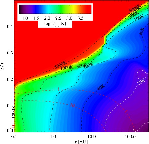
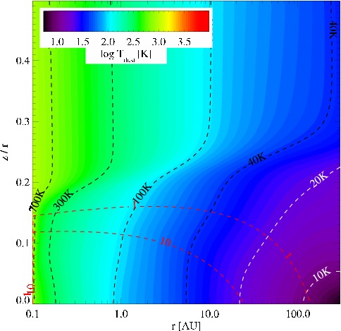
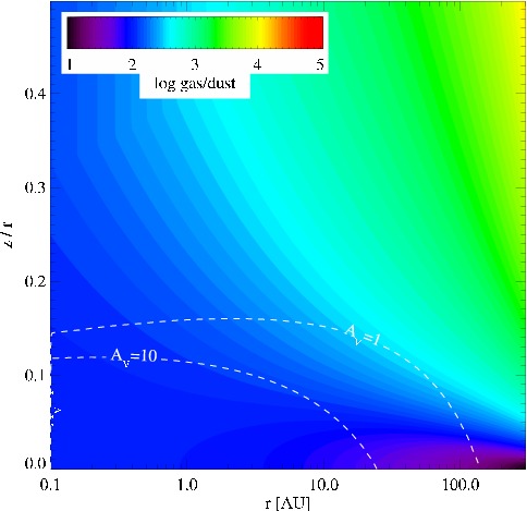
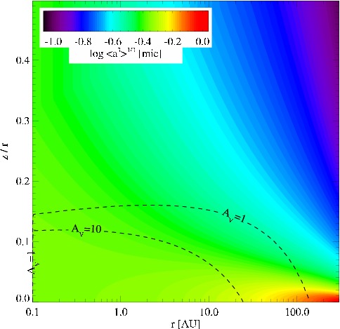
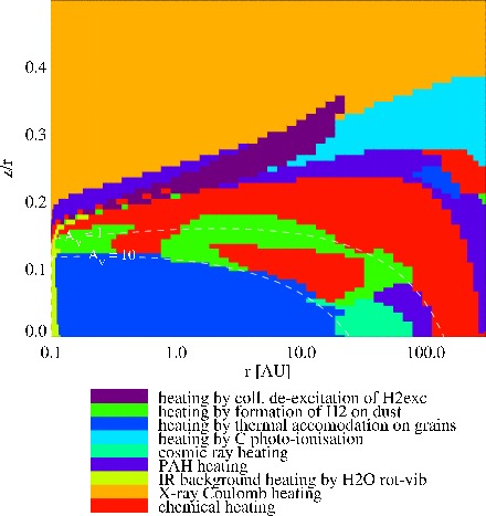
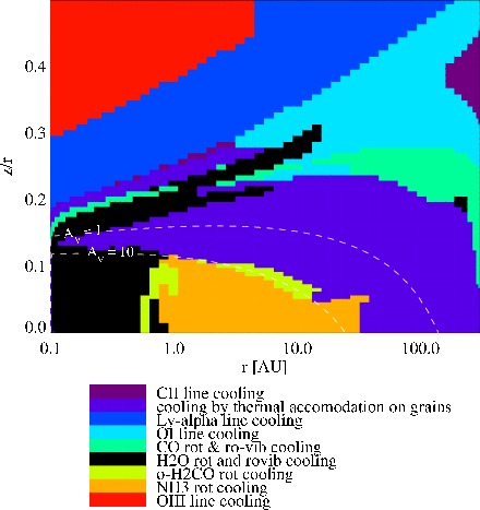
Figure 16: Standard model, from top to bottom and from left to right: $T_{\mathrm{gas}}$ with overplotted gas temperature contours (white/black) and $A_{\mathrm{V}}\leavevmode\nobreak\ =\leavevmode\nobreak\ 1,\leavevmode\nobreak\ 10$ (red), $T_{\mathrm{dust}}$ with overplotted temperature contours (black/white) and $A_{\mathrm{V}}\leavevmode\nobreak\ =\leavevmode\nobreak\ 1,\leavevmode\nobreak\ 10$ (red), dust-to-gas mass ratio, average dust grain size, main cooling processes (CII fine structure lines, dust grain-gas thermal exchange, Ly $\alpha$ line, neutral O line cooling, CO rotational and ro-vibrational cooling, water rotational and ro-vibrational cooling, formaldehyde rotational cooling, ammonia rotational cooling, OIII line cooling), main heating processes (collisional excitation of vibrationally excited H₂, chemical heating due to H₂ formation on dust grains, dust grain-gas thermal exchange, heating from the superthermal photo-electrons produced by C, heating by cosmic rays, heating by the photo-electrons produced by polycyclic aromatic hydrocarbons, IR heating due to the water transitions, heating by mutual electron collisions, Coulomb heating, produced by X-rays photoionization, reaction free energy heating from exothermic reactions).

The inner zone of the disk (A) is a warm reservoir with high density ($\geq$ 10⁹ cm^-3), which produces the Spitzer lines. Disk (A) zone is that with the largest water column density in the disk, and is extended from the inner wall up to the snow line. The lowest abundance gas reservoir is the outer reservoir (C). In this region, the density is below 100 cm^-3, and the optical depth is low. Hence, transitions from this cold outer region of the disk probe deeper into the disk; examples are the Herschel/HIFI lines as 538.29 $\mu$m and 269.27 $\mu$m. Reservoir C is extended from the outer end of the snow line (45 AU) up to the outer disk radius. The intermediate region above the ice is the reservoir B ($z/r\sim$ 0.1-0.25); it is radially extended between the reservoirs A and C. In this region, physical conditions (densities of H₂, H, e^-, temperatures of dust and gas) show large changes with radius. Many of the Herschel PACS and Spitzer Space Telescope high excitation lines (200 $<$ $E_{\mathrm{up}}$ $<$ 1000  K, not analyzed in this work) arise in this disk zone. Below this region, water is predominantly in the form of ice (I). The icy reservoir in Fig. 1 is here defined by a combination of the $T_{\mathrm{dust}}\leavevmode\nobreak\ \simeq\leavevmode\nobreak\ 100$ K line and the location of the continuum opacity $A_{\mathrm{V}}$ = 10. In the ice reservoir, the water abundances of the gas phase are depleted by 5 orders of magnitude with respect to the upper reservoir B. The ice reservoir can be indirectly probed through ice features arising from dust covered by mantles of frozen water. The 3 $\mu$m NIR ice feature has been detected by Terada et al. (2007), while McClure et al. (2012) reported the tentative detection of the 63 $\mu$m far-IR feature. Gas and dust are thermally coupled in the regions of the line emission of reservoir A and C (Fig. 16). In reservoir B, dust and gas temperatures are partially decoupled.

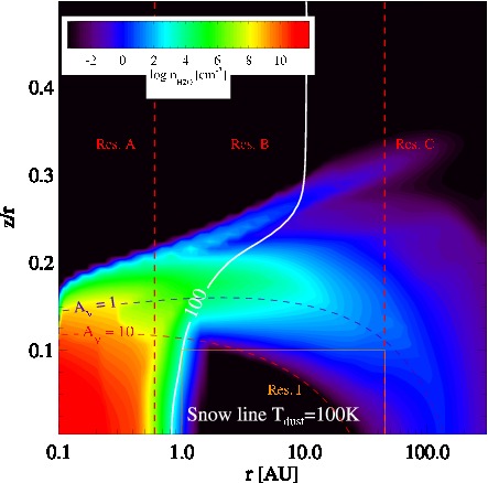
Figure 1: Water reservoirs in the standard disk; the white line represents the contour of $T_{\mathrm{dust}}\leavevmode\nobreak\ =\leavevmode\nobreak\ 100$ K, the black and red dashed curved lines represent the contours of optical extinction for $A_{\mathrm{V}}\leavevmode\nobreak\ =\leavevmode\nobreak\ 1$ and $A_{\mathrm{V}}\leavevmode\nobreak\ =\leavevmode\nobreak\ 10$, respectively. The water ice reservoir is outlined by the white contour and the dashed line corresponds to $A_{\mathrm{V}}\leavevmode\nobreak\ =\leavevmode\nobreak\ 10$. Vertical red dashed lines and the orange rectangle delimit the water reservoirs.

In general, dust settling produces a lower local dust content in the surface layers of all models (Fig. 16) and steepens the local dust power law distribution with respect to a completely unsettled case. The effect of settling is particularly relevant in the outer disk, where the mixing is not strong enough to stir up the dust grains. This makes the average grain size $\left<a\right>$ close to the midplane larger with respect to an unsettled model. In the line emitting region of the 12.407 $\mu$m water line (Fig. 2) for the standard model the average dust size is 0.45 $\mu$m, while in the region of the 538.29 $\mu$m this size drops to 0.36 $\mu$m. The standard model has a high mixing parameter, and is thus close to an unsettled disk model. In the water line emitting regions of all reservoirs ($z/r$ $\simeq$ 0.15-0.2), above the $A_{\mathrm{V}}\leavevmode\nobreak\ >$ 1 layer, chemical heating and H₂ formation heating are the main heating processes (Fig. 16). The cooling is dominated by H₂O rotational and ro-vibrational emission and CO rotational and ro-vibrational emission. Deeper in the disk, gas-grain collisions couple $T_{\mathrm{gas}}$ and $T_{\mathrm{dust}}$. Additional plots on the standard model properties can be found in Appendix B (Fig. 16).

3.1 Water chemistry

A complete list of the main reactions involving water in the disk model is reported in Table 4. The most important reactions in the emitting region of every transition are summarized in Table 5. They are sorted by their relevance with respect to the timescale and the number of grid points in which they dominate. The kinetical reaction constants of the gas phase are expressed in a parametrized manner with three coefficients ($\alpha$, $\beta$, $\gamma$). The calculation of the various types of reaction rates, using these coefficients, is described in Woodall et al. (2007) and Woitke et al. (2009a).

Table 3: Main reaction channels in order or relevance for water formation and destruction in the standard disk model

Reaction number	Reaction	$\rm\alpha$ [cm3 s-1] or [s-1]	$\rm\beta$ [-]	$\rm\gamma$ [K]	Type	References
1	H2 + OH $\rightarrow$ H2O + H	2.05$\times 10^{-12}$	1.52	1740.00	Neutral-Neutral	1
2	NH + OH $\rightarrow$ H2O + N	3.11$\times 10^{-12}$	1.20	0.00	Neutral-Neutral	2,1
3	NH2 + OH $\rightarrow$ H2O + NH	7.78$\times 10^{-13}$	1.50	-230.00	Neutral-Neutral	1
4	NH2 + NO $\rightarrow$ N2 + H2O	4.27$\times 10^{-11}$	-2.50	331.00	Neutral-Neutral	2,1
5	OH + OH $\rightarrow$ H2O + O	1.65$\times 10^{-12}$	1.14	50.00	Neutral-Neutral	3
6	OH + H2CO $\rightarrow$ HCO + H2O	2.22$\times 10^{-12}$	1.42	-416.00	Neutral-Neutral	1
7	NH2 + H3O+ $\rightarrow$ H2O + NH${}_{3}^{+}$	9.70$\times 10^{-10}$	0.00	0.00	Ion-Neutral	4
8	H3O+ + Si $\rightarrow$ SiH+ + H2O	1.80$\times 10^{-9}$	0.00	0.00	Ion-Neutral	4
9	H3O+ + SiO $\rightarrow$ SiOH+ + H2O	2.00$\times 10^{-9}$	0.00	0.00	Ion-Neutral	5
10	H3O+ + e- $\rightarrow$ H2O + H	1.08$\times 10^{-7}$	-0.50	0.00	Dissociative Recombination	6
11	H- + OH $\rightarrow$ H2O + e-	1.00$\times 10^{-10}$	-5.22	90.00	Associative Detachment	4
12	H + OH $\rightarrow$ H2O + h$\nu$	5.26$\times 10^{-18}$	-5.22	90.00	Radiative Association	7
13	H3O+ + h$\nu$ $\rightarrow$ H2O + H+	2.00$\times 10^{-11}$	0.00	2.00	Photodissociation	8
14	H${}_{2}^{*}$ + OH $\rightarrow$ H2O + H	3.60$\times 10^{-11}$	0.00	0.00	Neutral-Neutral(a)	1
15	H2O(ice) + dust $\rightarrow$ H2O + dust	-	-	4800.00	Desorption(b)	9,19
16	H2O(ice) + C.R.P. $\rightarrow$ H2O + dust	-	-	4800.00	Cosmic-rays-desorption(b)	19
17	H2O(ice) + h$\nu$ $\rightarrow$ H2O	-	-	4800.00	Photodesorption(b)	9,19
18	PAH- + H3O+ $\rightarrow$ PAH + H2O + H	1.70$\times 10^{-8}$	0.50	0.00	PAH Dissociative Recombination	18
1	H2O + H $\rightarrow$ OH + H2	1.59$\times 10^{-11}$	1.20	9610.00	Neutral-Neutral	1
2	H${}_{3}^{+}$ + H2O $\rightarrow$ H3O+ + H2	5.90$\times 10^{-9}$	0.00	0.00	Ion-Neutral	10
3	C+ + H2O $\rightarrow$ HCO+ + H	9.00$\times 10^{-10}$	0.00	0.00	Ion-Neutral	4
4	CH${}_{5}^{+}$ + H2O $\rightarrow$ H3O+ + CH4	3.70$\times 10^{-9}$	0.00	0.00	Ion-Neutral	10
5	H2O + Si+ $\rightarrow$ SiOH+ + H	2.30$\times 10^{-10}$	0.00	0.00	Ion-Neutral	11
6	H2O + HCO+ $\rightarrow$ CO + H3O+	2.50$\times 10^{-9}$	0.00	0.00	Ion-Neutral	12
7	H2O + HN${}_{2}^{+}$ $\rightarrow$ N2 + H3O+	2.60$\times 10^{-9}$	0.00	0.00	Ion-Neutral	13
8	H2O + SiH+ $\rightarrow$ Si+ + H3O+	8.00$\times 10^{-10}$	0.00	0.00	Ion-Neutral	5
9	H+ + H2O $\rightarrow$ H2O+ + H	6.90$\times 10^{-9}$	0.00	0.00	Charge Exchange	14
10	He+ + H2O $\rightarrow$ He + H2O+	6.05$\times 10^{-11}$	0.00	0.00	Charge Exchange	15
11	H2O + h$\nu$ $\rightarrow$ OH + H	5.90$\times 10^{-10}$	0.00	1.70	Photodissociation	16
12	H2O + h$\nu$ $\rightarrow$ H2O+ + e-	3.30$\times 10^{-11}$	0.00	3.90	Photoionization	16
13	H2O + dust $\rightarrow$ H2O(ice)	-	-	-	Adsorption(b)	19
14	Ne+ + H2O $\rightarrow$ Ne + H2O+	8.00$\times 10^{-10}$	0.00	0.00	Charge Exchange	17

(1) Mallard, W. G., Westley, F., Herron, J.T., Hampson, R.F., Frizell, D.H. (1994); (2) McElroy et al. (2013); (3) Woodall et al. (2007); (4) Prasad & Huntress (1980); (5) Herbst et al. (1989); (6) Tielens & Hollenbach (1985); (7) Field et al. (1980); (8) Jensen et al. (2000); (9) Hollenbach & Gorti (2009); (10) Kim & Huntress (1975); (11) Fahey et al. (1981); (12) Adams et al. (1978); (13) Rakshit (1982); (14) Smith et al. (1992); (15) Mauclaire et al. (1978); (16) van Dishoeck et al. (2006); (17) Anicich (1993); (18) Flower & Pineau des Forêts (2003); (19) Aikawa et al. (1996)

Table 4: Main reaction channels in the emitting regions of the considered transitions in the standard model

Species & wavelength [$\rm\mu m$]	Formation reaction number	Destruction reaction number
o-H2O 12.396	1,10	1,11
p-H2O 12.407	1,10	1,11
o-H2O 12.445	1,10	1,11
o-H2O 12.453	1,10	1,11
p-H2O 12.832	1,10	1,11
p-H2O 12.894	1,10	1,11
o-H2O 33.510	1,10,4	1,11
p-H2O 269.27	12,10,4	12,10,13,11,5
o-H2O 538.29	12,10,4	12,10,13,11,5

The emitting regions of the Spitzer transitions (except the 33.510 $\mu$m line) are co-spatial (Fig. 2). Hence the main processes and chemical rates are very similar. For these transitions, the main formation channels are the neutral-neutral reactions of H₂ and OH, and due to the presence of X-rays, the dissociative recombination of H₃O⁺. For the 33.510 $\mu$m line, there is an additional neutral-neutral nitrogen chemistry channel via NH₂ and NO. The reaction rates (for a two-body reaction, $k_{\mathrm{i,j}}\cdot n_{\mathrm{i}}\cdot n_{\mathrm{j}}$ [s^-1]) in these dense and hot regions of the disk are above 10³ s^-1. Water in these regions is chemically mainly depleted through neutral-neutral reactions involving atomic hydrogen and through photodissociation.

In the outer disk (reservoir C), water is produced mainly through dissociative recombination of H₃O⁺ and radiative association of OH and H. Secondary formation channels are the neutral-neutral reactions involving NO and NH₂. In this reservoir, several processes deplete water vapor: photoionization, charge exchange with He⁺ and ion-neutral reaction with Si⁺ (driven by X-rays, cosmic rays and collisional ionization with electrons), water photodissociation, and ice formation. The reaction rates here are lower than in reservoir A, of the order of 10^-5 s^-1 ($\sim$ 1 day), but the timescales are still shorter than the disk lifetime.

Previous studies found differences in terms of nitrogen chemistry for T Tauri disks. The channels mentioned above are an important formation path for water precursors (as OH) in the outer disk of TW Hya, and in a tiny region in the inner rim where water is directly formed from NO and NH₂ (Kamp et al., 2013). In the Najita et al. (2011) chemistry network, atomic nitrogen is a competitor that depletes OH in the disk atmosphere, making it harder to produce water. However, this model only includes X-rays and not FUV and also lacks water rotational cooling. Water in the inner disk is formed through the activated channel involving OH and H₂, in agreement with our modeling. The Glassgold et al. (2009) model does not include FUV and its network is limited to 125 reactions and 25 species, including only H, He, C, and O. This model agrees with our study on the water formation mechanism through neutral-neutral reaction of OH and H₂, and finds that reactions with H⁺ are the main destruction channels of water in the upper layers.

In the modeling of Herbig disks, performed with a comparable chemical network, Woitke et al. (2009b) found that dissociative recombination is not important in the inner disk, contrary to the case of T Tauri disks. The outer disk water reservoir of Herbigs is then fueled by photodesorption processes from the ices, while the depletion is again due to photodissociation. The main difference from the chemistry in T Tauri disks is the lack of channels involving ions.

3.2 Water spectroscopy

Water has an extremely rich spectroscopy, making it necessary to select a subsample of lines for this study. We thus focus here on the list of transitions shown in Table 5, which are based on Spitzer and Herschel/HIFI line detections in disks around T Tauri stars. A detailed investigation of each single line regarding the chemistry is only performed for the reference model (parameters are reported in boldface in Table 2).

Table 5: Water lines selected for this work

Species	Wavelength [$\mu$m]	Instrument	Reservoir	$E_{\mathrm{up}}$ [K]	Quantum numbers $v_{\mathrm{1}}v_{\mathrm{2}}v_{\mathrm{3}}JK_{\mathrm{a}}$ $K_{\mathrm{c}}$
p-H2O	12.407	Spitzer IRS	A	4945.0	000-000 16-15 3-2 13-14
o-H2O	12.396	Spitzer IRS	A	5781.0	000-000 17-16 4-3 13-14
o-H2O	12.445	Spitzer IRS	A	3629.0	000-000 11-10 8-5 3-6
o-H2O	12.453	Spitzer IRS	A	4213.0	000-000 13-12 7-4 6-9
p-H2O	12.832	Spitzer IRS	A	3243.0	000-000 10-9 8-5 2-5
p-H2O	12.894	Spitzer IRS	A	3310.0	000-000 12-11 5-2 7-10
o-H2O	33.510	Spitzer IRS	A/B	2275.0	000-000 10-9 4-3 7-6
p-H2O	269.27	Herschel HIFI	B/C	53.43	000-000 1-0 1-0 1-0
o-H2O	538.29	Herschel HIFI	B/C	60.96	000-000 1-1 1-0 0-1

The mid-IR transitions originate from the warmest water reservoir (A, Fig. 2), consistent with their high upper level energies (Table 5). The two sub-mm lines are produced in the outer cold disk (reservoir C). We chose the mid-IR 12 $\mu$m lines because they are also observable from the ground with VISIR on the VLT (Pontoppidan et al., 2010a) and they are physically unblended. This last aspect is very important, because our modeling is based on individual line radiative transfer. The strongest detections in the Spitzer regime are the blends around 15 $\mu$m and 17 $\mu$m (Pontoppidan et al., 2010b; Carr & Najita, 2011; Zhang et al., 2013), but the difference from the 12 $\mu$m lines is within a factor 10. We verified that the behavior of the single components of the blends in the Pontoppidan et al. (2010b) work is the same as that of the individual lines we discussed. In the following, we plot all the line fluxes as a function of the selected parameters. The focus of this study is to understand the discrepancy in detection between Spitzer/IRS and Herschel/HIFI, i.e., between the inner and outer disk, and to find a possible connection/explanation with the physical properties of the disks.

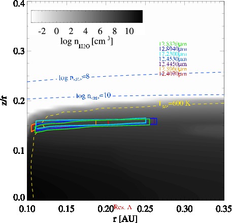
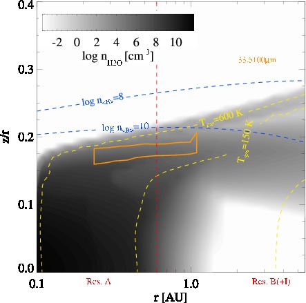
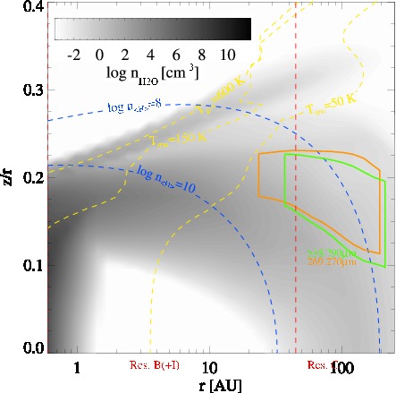
Figure 2: Water lines from different reservoirs in the standard model; left: reservoir A, center: reservoir A-B, right: reservoir B-C. the blue dashed curved lines are contours for gas densities of 10⁸ and 10¹⁰ cm^-3, the yellow contours are for gas temperatures of 50 K, 150 K, 600 K. Vertical red dashed lines delimit the reservoirs.

Fig. 2 shows the observed and detected Spitzer lines considered here; ($E_{\mathrm{up}}\leavevmode\nobreak\ \geq\leavevmode\nobreak\$3000 K). Since reservoir A is very compact compared to the disk size, these transitions largely overlap in their emitting volume, and as a consequence, the physical conditions are very similar for all the lines. As long as the radial and vertical temperature and density gradients in these line emitting regions are small, a simplified slab approach as employed, e.g., in Carr & Najita (2008) presents a reasonable approximation. The transitions below 12.5 $\mu$m are produced in a region that is partially optically thick. A vertical integration of the dust extinction (see Appendix A) confirms that the $\tau_{\mathrm{dust}}$ = 1 surface at the wavelength of the line is above the mean vertical height of the line emitting region, so that the lines are partially buried in the continuum. Lines from reservoir B are produced in an optically thinner region, about 50% of the emitting region is optically thin. More than 30% of the 269.27 $\mu$m and 70% of the 538.29 $\mu$m line emitting regions (reservoir C) are vertically extended above the $\tau_{\mathrm{dust}}\leavevmode\nobreak\ =\leavevmode\nobreak\ 1$ contour at the respective wavelengths.

The far-IR transitions are very close to LTE because the average density of H₂ is close to the critical density (within an order of magnitude), and so we expect them to be sensitive to $T_{\mathrm{gas}}$ and $n_{\mathrm{gas}}$ variations. Our mid-IR lines, instead, are produced in a very dense region of the disk, and so they form under LTE conditions. Table 6 shows that H₂ is the main collisional partner for all considered transitions because the H/H₂ ratio is always below 0.1. Because of changes in the physical conditions of the different models, the previous statements are strictly valid only for our standard disk model.

Table 6: Overview and coefficients of the considered transitions

species	wavelength [$\mu$m]	$A_{\mathrm{ul}}$ [s-1]	$\left<n_{\mathrm{H_{2}}}\right>C_{\mathrm{H_{2},ul}}^{\mathrm{(a)}}$ [s-1]	$\left<n_{\mathrm{H}}\right>C_{\mathrm{H,ul}}^{\mathrm{(a)}}$ [s-1]	$\left<n_{\mathrm{e^{-}}}\right>C_{\mathrm{e^{-},ul}}^{\mathrm{(a)}}$ [s-1]
p-H2O	12.407	4.217	4.489$\times 10^{12}$ (o & p)	2.838$\times 10^{9}$	8.918$\times 10^{-3}$
o-H2O	12.396	7.665	4.823$\times 10^{12}$ (o & p)	3.076$\times 10^{9}$	1.757$\times 10^{-2}$
o-H2O	12.445	2.937$\times 10^{-1}$	4.982$\times 10^{11}$ (o & p)	2.990$\times 10^{8}$	4.089$\times 10^{-4}$
o-H2O	12.453	1.160	1.660$\times 10^{12}$ (o & p)	9.963$\times 10^{8}$	1.431$\times 10^{-3}$
p-H2O	12.832	1.564$\times 10^{-1}$	1.375$\times 10^{12}$ (o & p)	8.253$\times 10^{8}$	2.399$\times 10^{-4}$
p-H2O	12.894	2.596$\times 10^{-1}$	5.856$\times 10^{11}$ (o & p)	3.154$\times 10^{8}$	3.956$\times 10^{-4}$
o-H2O	33.510	4.691	1.877$\times 10^{11}$ (o & p)	6.689$\times 10^{7}$	2.862$\times 10^{-2}$
p-H2O	269.27	1.852$\times 10^{-2}$	1.817$\times 10^{-3}$ (para) 7.943$\times 10^{-3}$ (ortho)	1.070$\times 10^{-6}$	4.145$\times 10^{-5}$
o-H2O	538.29	3.477$\times 10^{-3}$	1.348$\times 10^{-3}$ (para) 1.274$\times 10^{-2}$ (ortho)	5.985$\times 10^{-7}$	5.869$\times 10^{-5}$

4 Results

The previously discussed standard model is a starting point from which we build a series of models, modifying a single parameter per disk model. In the following, we discuss the results from this series.

The line fluxes have been treated as independent transitions, hence, as physically unblended. The results reported here are based on vertical escape probability. This approach agrees within a factor of two with a more detailed and computationally more expensive radiative transfer (Fig. 3). In particular, far-IR lines agree within 30%, while mid-IR lines agree within 70%. The lines from vertical escape probability show a systematical stronger value than detailed RT lines. The reason for this mismatch is twofold: the disk inclination (30 $\deg$) causes larger column densities of gas and dust in the detailed RT calculation with respect to the vertical escape treatment. In addition, the vertical escape does not take the line self-absorption into account. The vertical escape method is a fast and powerful method to compute tens of thousands of lines for different species. Cases in which the vertical escape probability is unreliable are rare cases of absorption lines. Those are limited to very few flat models ($\beta\leavevmode\nobreak\ <\leavevmode\nobreak\ 0.8$), to models with $a_{\mathrm{pow}}\!\geq\!4.0,$ or dust-to-gas mass ratio $\geq$ 100, and our conclusions are not affected.

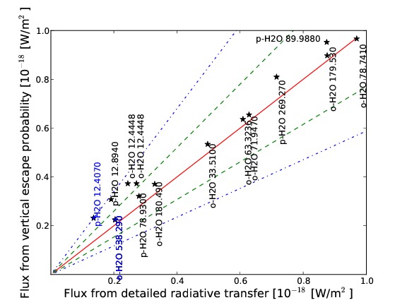
Figure 3: Comparison between the vertical escape probability flux and a detailed radiative transfer computation for the standard model. Green dashed and blue dot-dashed lines are confidence intervals of 30% and 70% from the red line, respectively.

To illustrate the results, the theoretical Spitzer spectrum of each model is computed with a resolution of 600 (the maximum of IRS, of LH and SH modules; Houck et al., 2004). These spectra give a first qualitative result, which can be compared to observations. We also define a “mid-IR color” as the ratio of the continuum fluxes at 13.5 and 30 $\mu$m as indicator of the SED slope in the Spitzer wavelength range.

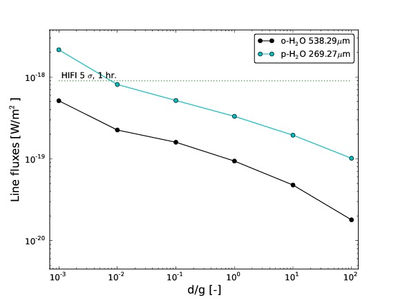
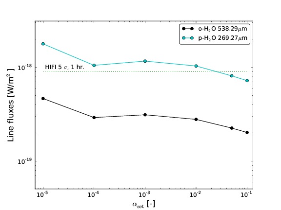
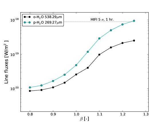
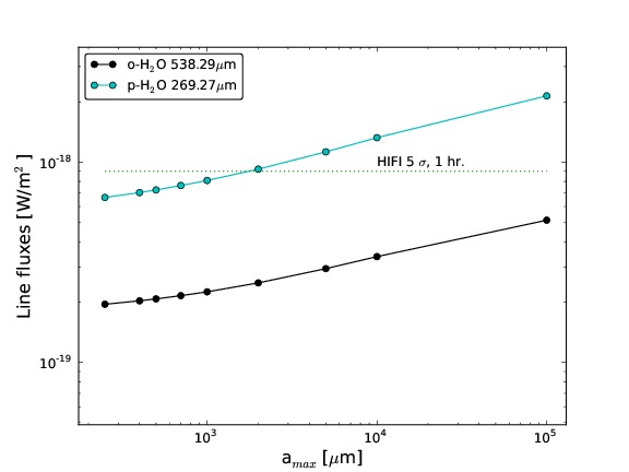
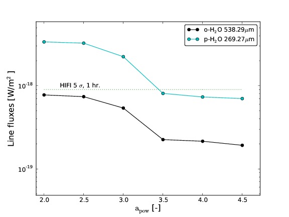
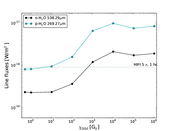
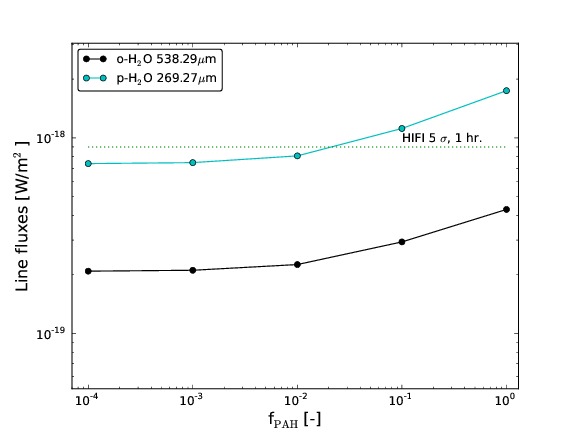
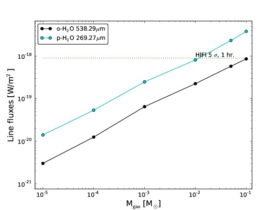
Figure 15: Line fluxes behavior for Herschel/HIFI lines 538.29 $\rm\mu m$ and 269.27 $\rm\mu m$ for different model series. First row left: dust-to-gas mass ratio, $d/g$. First row right: mixing parameter, $\alpha_{\mathrm{set}}$. Second row left: disk flaring, $\beta$. Second row right: maximum grain size a_max. Third row left: power law index of grain size distribution, $a_{\mathrm{pow}}$. Third row right: strength of UV radiation field, $\chi_{\mathrm{ISM}}$. Third row left: PAH abundance, $f_{\mathrm{PAH}}$. Bottom right: disk gas mass, $M_{\mathrm{gas}}$.

In the following subsections, we discuss the behavior of the selected transitions, considering the representative mid-IR and far-IR lines. We also describe in detail some average physical quantities in the line emitting regions. The computation of these quantities is described in detail in Appendix A. We compare the predicted fluxes with the sensitivity limits for Spitzer/IRS ($5\cdot 10^{-18}$ W/m², 1 $\sigma$, deduced from the typical upper limits; Pontoppidan et al., 2010b), Herschel/HIFI ($9\cdot 10^{-19}$ W/m², 1 hr, 5 $\sigma$; de Graauw, 2004), and finally JWST/MIRI (10^-20 W/m², 2.7 hrs., 10 $\sigma$; Glasse et al., 2010). Additional plots with the 538.29 $\mu$m o-H₂O line flux and line ratios 538.29 $\mu$m/12.407 $\mu$m are included in Appendix B (Fig. 15 & 17).

4.1 Dust-to-gas mass ratio

A variation of this parameter means changing the dust mass since the gas mass is fixed to 0.01 M_⊙.

The water total column densities in the inner disk are unaffected by the dust content (Fig. 4b). However, the Spitzer line at 12.4 $\mu$m is produced by a volume in which the column density is suppressed up to 14 orders of magnitude from the low to high dust-to-gas mass ratio (Fig. 4a). The emitting region of the Spitzer line becomes radially more extended between the low and high dust-to-gas case (Fig. 4c). This is because the total water reservoir is unaffected, while the emitting region moves upward to the disk surface with increasing dust mass (Fig. 4c); this causes the densities in the emitting region to drop by 8 orders of magnitude. The continuum opacity in the line emitting region grows with increasing dust mass (Fig. 4h).

In summary, mid-IR line fluxes are driven indirectly by the increase in dust opacity; it forces the lines to move upward in the disk into lower density regions (Fig. 4c & h). The continuum optical depth increase reduces the column density of emitting water. The deviation beyond a dust-to-gas ratio of 10.0 is due to the extremely optically thick disk, which forces the lines to be produced from more optically thin surface layers beyond 0.5 AU.

In the outer disk, which hosts the ice reservoir, changes in the opacity affect the photoevaporation process, increasing the total water vapor column density (Fig. 4b). The emitting region of the fundamental water lines gets progressively close to $A_{\mathrm{V}}\leavevmode\nobreak\ =\leavevmode\nobreak\ 1$. The emitting region’s radial displacement with the increase of dust mass is less pronounced than in the mid-IR case (Fig. 4c), but the vertical displacement is significant. Also, the line flux of the far-IR water lines is driven by an opacity effect, but to a lesser extent compared to the mid-IR. Also, the emitting region moves upward with increasing dust mass, however, the emitting water column density is only reduced by two orders of magnitude between the most extreme models (Fig. 4a). The situation is less extreme, because the outer disk is only marginally optically thick (Fig. 4a).

(a)

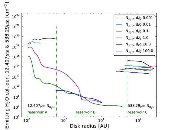
(b)

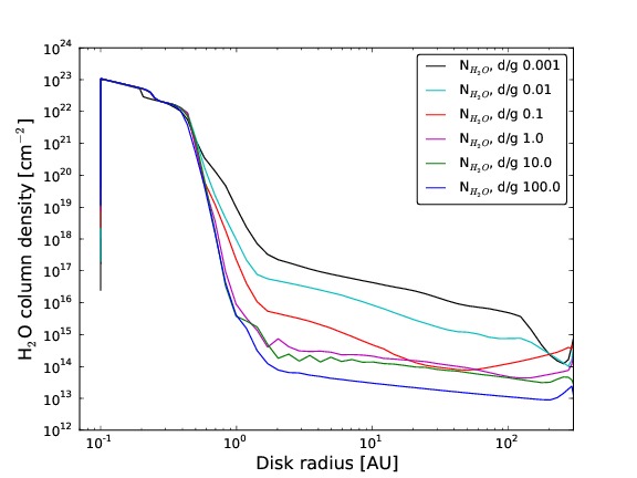
(c)

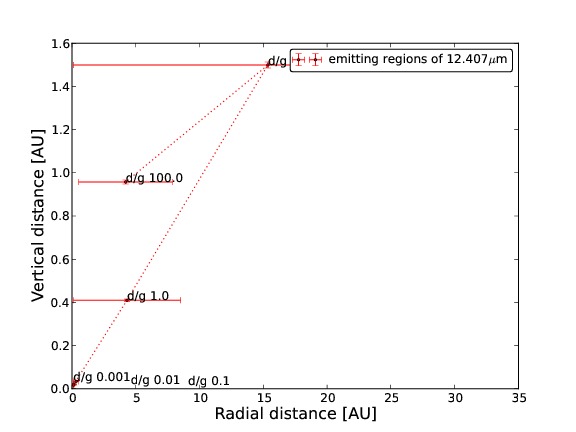
(d)

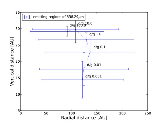
(e)

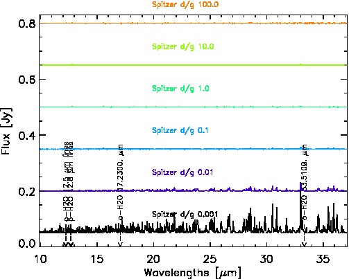
(f)

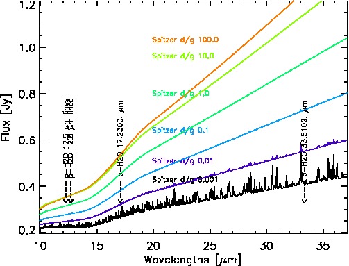
(g)

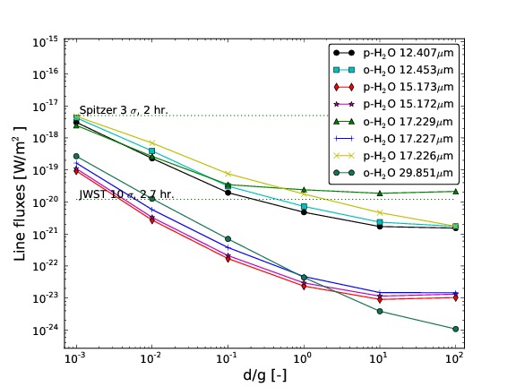
(h)

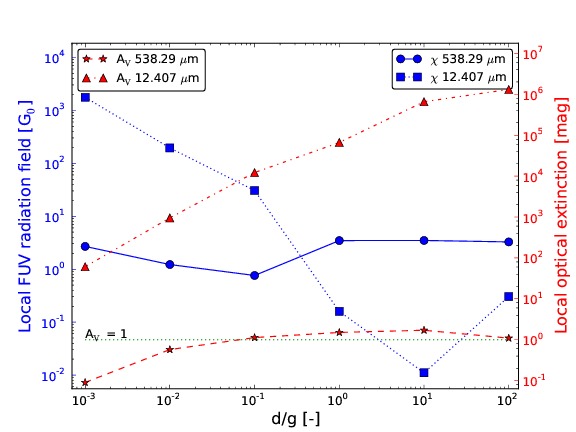
Figure 4: Plots for dust-to-gas mass ratio models. (a) Emitting region water column density comprises 15-85% of the radially and vertically integrated flux. Vertical dotted green lines distinguish the reservoirs. (b) Total water column densities as a function of radius. (c) Average extension of the line emitting region that comprises 50% of the line flux radially and vertically for 12.407 $\mu$m. (d) Average extension of the line emitting region for 538.29 $\mu$m (50% of radially and vertically integrated flux). (e) Theoretical Spitzer SH/LH modules spectra ($R$ = 600) for this model series, continuum subtracted and arbitrarily shifted. (f) Theoretical Spitzer SH/LH modules spectra ($R$ = 600) for this model series. (g) Spitzer line fluxes with sensitivity limits (green dotted lines) for Spitzer/IRS, JWST/MIRI. (h) Radiation field and optical extinction in the line emitting regions of 12.407 $\mu$m and 538.29 $\mu$m.

All Spitzer transitions show a strong dependence on the dust-to-gas mass ratio (Fig. 4e & f). The line-to-continuum ratio changes by a factor 2.5 between the smallest and largest dust-to-gas ratio, and in the dust-rich models all line features disappear from the Spitzer/IRS spectra. This is in agreement with previous results of Meijerink et al. (2009). The continuum fluxes decrease with decreasing dust content, and the 13.5/30 $\mu$m continuum flux ratio decreases with increasing dust content in the disk.

4.2 Dust settling

Settling affects the water spectroscopy much less than the dust-to-gas mass ratio. In fact, the largest systematic difference in water column density can be found in the outer disk, $r\!>$ 10 AU (Fig. 5b). The Spitzer emitting region only shows a change in the water emitting column density in the most settled model; that is also the only one producing a slightly stronger line flux (Fig. 5g). The most settled model has a higher column density in the water emitting regions of the mid-IR and far-IR lines because of the reduced continuum opacity that boosts the thermally activated water formation channels. In the inner disk, the density is very high, and therefore the dust is largely unsettled. In cases of extremely low mechanical mixing only($\alpha_{\mathrm{set}}\!\leq\!10^{-5}$), the disk has such a low opacity that the line emitting region moves upward because of increased radial extension in the disk, and the column density of the emitting region is higher than in an unsettled case (Fig. 5b). In the emitting region of the far-IR lines, the column density is more affected (Fig. 5b); for $\alpha_{\mathrm{set}}\!<\!0.01$, the total water column density grows about an order of magnitude (Fig. 5d). Because of the migration of the far-IR line emitting region, dust extinction fades quickly from a marginally optically thick regime to an optically thin regime (Fig. 5h). The outer disk is affected by settling only for $\alpha_{\mathrm{set}}\!<\!10^{-3}$; this threshold can be found in the evolution of several properties, such as the opacity (Fig. 5h).

In the outer disk the photodesorption of water (Sect. 3.1) and photodissociation processes are not strong enough to deplete water significantly. This produces an upward migration of the emitting region for the far-IR transition in the most settled models. The Spitzer line emitting region migration (Fig. 5c) and larger emitting water column density are negligible given numerical uncertainties.

(a)

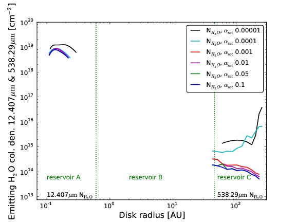
(b)

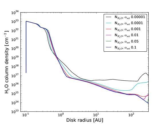
(c)

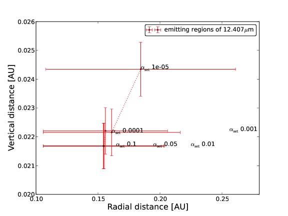
(d)

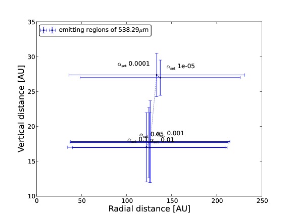
(e)

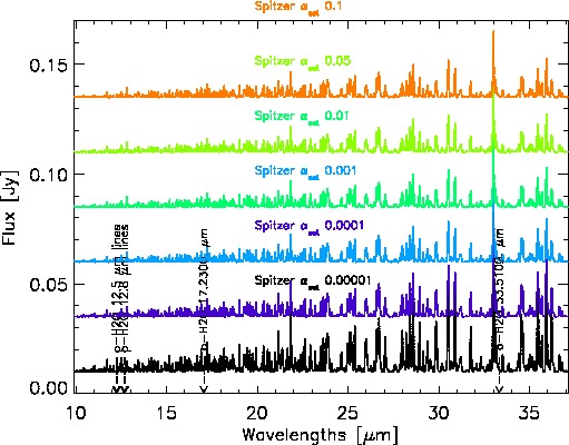
(f)

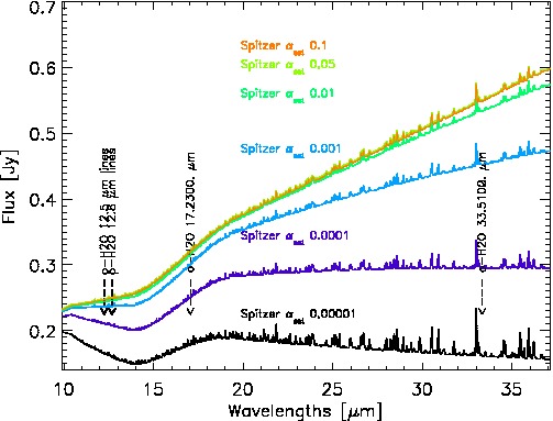
(g)

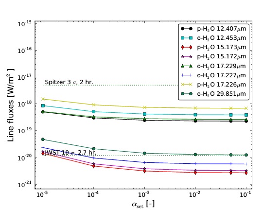
(h)

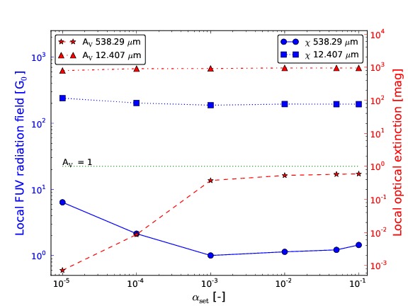
Figure 5: Plots for mixing coefficient models. For further details see Fig. 4.

The reduction of the mixing parameter produces a moderate enhancement in the mid-IR line-to-continuum ratio (Fig. 5e & f), along with a reduction of the continuum flux because of the decrease of dust in the surface layers of the inner disk. The 13.5/30.0 $\mu$m continuum flux ratio decreases with increasing the mixing coefficient $\alpha_{\mathrm{set}}$.

4.3 Flaring parameter $\beta$

In the parametrized modeling, the disk structure can be set through the scale height at a reference radius $H_{\mathrm{0}}$ and the flaring index $\beta$. Here, we only change the flaring and fix the scale height at the inner disk radius. A value of $\beta\!<\!1.0$ produces a disk collapsed vertically behind the inner radius and completely shadowed by the vertical extent of the inner disk rim.

(a)

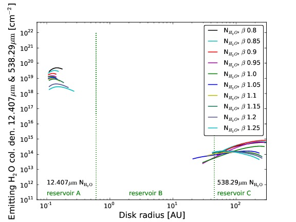
(b)

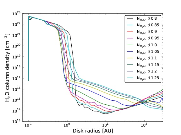
(c)

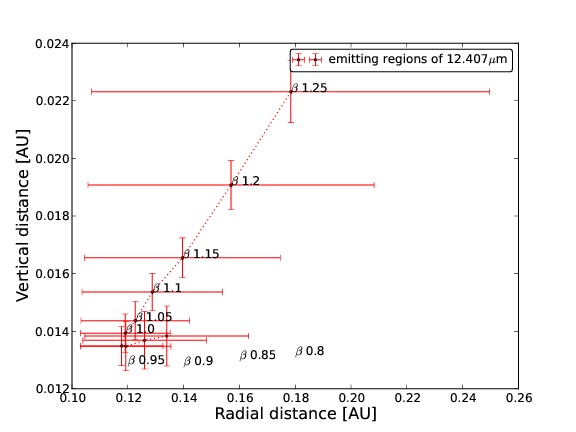
(d)

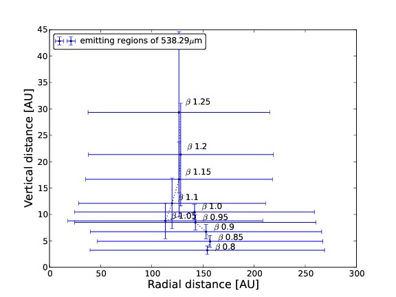
(e)

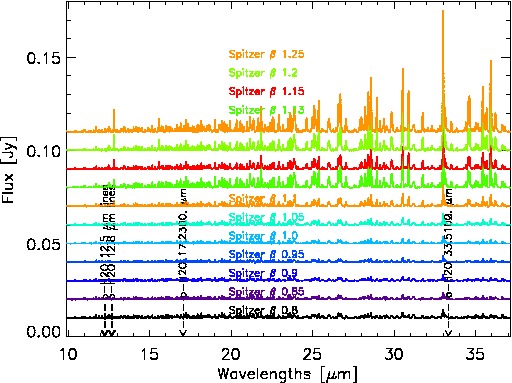
(f)

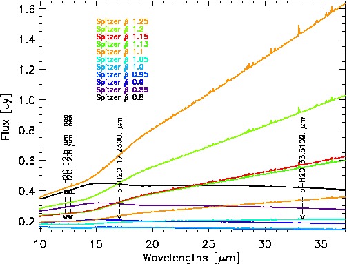
(g)

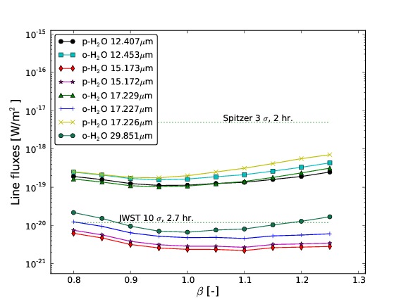
(h)

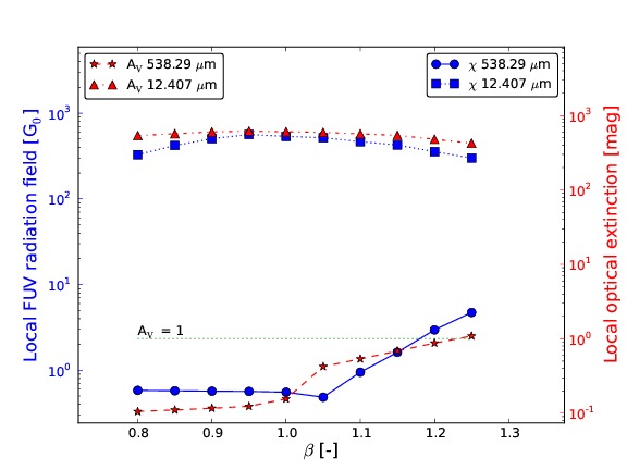
Figure 6: Plots for flaring index exponent models. For further details see Fig. 4.

An increasing flaring index decreases the water column density of the emitting region by up to two orders of magnitude, and the emitting region becomes up to a factor 1.5 more radially extended (Fig. 6h). As consequence of the increased radial extension, the emitting region of the Spitzer lines also moves upward with increasing flaring index (Fig. 6c). The line fluxes show a minimum for $\beta\leavevmode\nobreak\ =\leavevmode\nobreak\ 1.0$ (Fig. 6g) and increase for $\beta\leavevmode\nobreak\ >\leavevmode\nobreak\ 1.0$ up to a factor 1.5. The mid-IR spectral changes can be explained by a pure geometrical effect. Although the variation in the inner disk is small (since the inner disk scale height is fixed), it is enough to increase the heating of the surface layers of the inner disk to the central star radiation.

The outer disk total water column density is more affected than the inner disk, and the total amount of water (beyond 80 AU) is a factor $\sim$ 2 larger in the most flared case with respect to the flattest case (Fig. 6b). With increasing flaring, the emitting region moves upward and gets vertically more extended (Fig. 6d) because of an increase of the line opacity. The column density of water vapor in the emitting region becomes smaller, but the $T_{\mathrm{gas}}$ becomes larger. This is consistent with the monotonic increase of the Herschel/HIFI line flux.

With increasing flaring, the disk surface is irradiated more strongly by the central star. This increases the dust temperature through the entire disk (especially in the surface layers) and hence the mid-IR color value decreases (Fig. 6f).

4.4 Maximum grain size

The total column density of water beyond 1 AU is affected by the maximum grain size; the models with bigger grains have a larger water vapor column density (Fig. 7b). The lower the opacity, the more depleted is the ice reservoir, both vertically and radially, thus enriching the gas phase. The water column density in the emitting region of the Spitzer transition also increases (Fig. 7a). That region moves upward and becomes more extended with increasing maximum grain size (Fig. 7 g). Since the total dust mass remains constant with increasing $a_{\mathrm{max}}$, the population of small grains is reduced. As a consequence, the average continuum opacity (Fig. 7h) in the emitting region decreases with the increase of maximum grain size because the radial gas and dust temperature gradient flattens and the emitting region becomes radially more extended. This is a consequence of the increased FUV flux through the whole disk. The vertical displacement is a consequence of a radially more extended emitting region because the disk is flared and the emitting region moved outward also becomes more extended vertically (Fig. 7c). The mid-IR line fluxes increase monotonically with increasing maximum dust size because of increased emitting area and lower continuum opacity (Fig. 7c & h).

The emitting region of the Herschel lines (Fig. 7d) moves closer to the midplane of the disk for larger $a_{\mathrm{max}}$, maintaining roughly the same radial extent and position (Fig. 7d). This is again due to the lower dust optical depth for the models with larger grains. The water column density increase with increasing $a_{\mathrm{max}}$ translates into larger fluxes since the lines are optically thin.

(a)

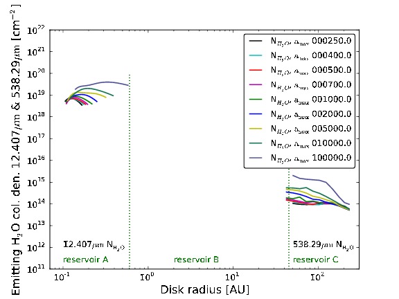
(b)

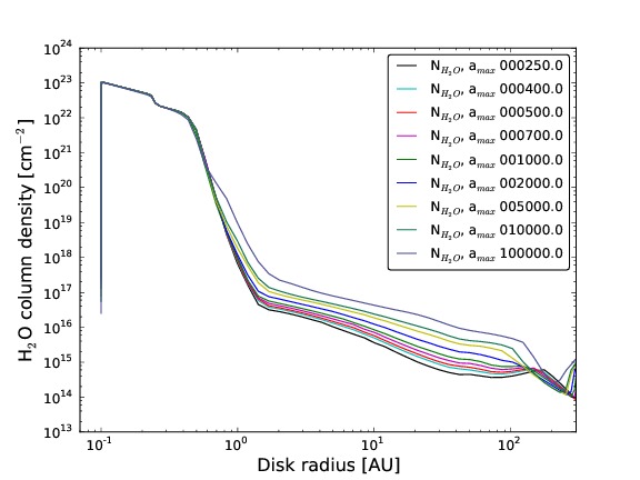
(c)

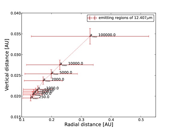
(d)

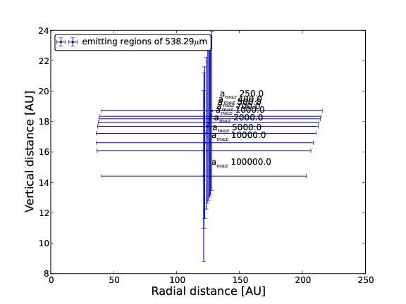
(e)

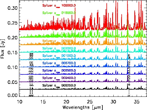
(f)

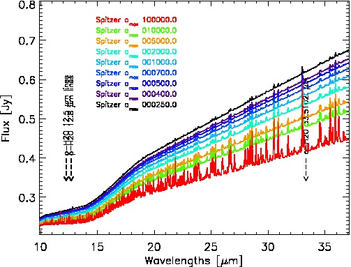
(g)

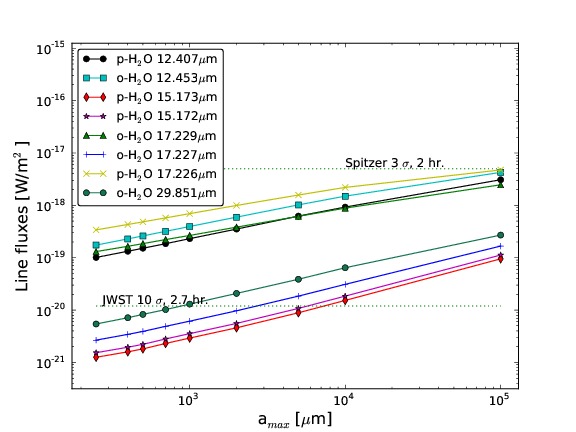
(h)

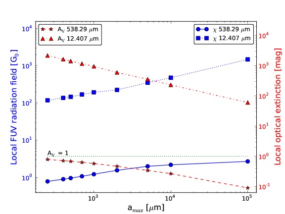
Figure 7: Plots for maximum dust size models. For further details see Fig. 4.

The modeled Spitzer spectrum (Fig. 7e & f) shows a decreasing mid-IR dust continuum for models with larger maximum grain sizes. There is, however, no significant variation of mid-IR color (within a factor 2).

4.5 Dust size power law distribution

The total water column density inside 1 AU remains constant when varying the power law index of the grain size distribution, while it decreases by several orders of magnitude in the outer disk (Fig. 8b). The water column density in the Spitzer line emitting region becomes lower, and the region shrinks radially by more than a factor of 3 (Fig. 8a & c). The migration is, however, not monotonic (Fig. 8c). This is because in the models with a power law index above 3.0, the continuum optical depth in the Spitzer emitting region increases strongly. Below 3.0, the optical depth stays constant ($\tau_{\mathrm{cont}}\!\sim\!100$). The increase in opacity causes the line emitting region to move inward, where the gas still reaches the line excitation temperatures.

In the Herschel/HIFI emitting region, dust and gas are thermally coupled above a threshold of $a_{\mathrm{pow}}\!=\!3.5$. The emitting region becomes progressively optically thick for larger $a_{\mathrm{pow}}$, but it never reaches $A_{\mathrm{V}}\!=\!1$. The line is emitted deeper in the disk in the models with $a_{\mathrm{pow}}\!=$ 2.0 up to 3.0. This is due to enhanced photodesorption, which increases the water column density in the sub-mm line emitting region. The lower column densities of water vapour in the outer disk lead to lower fluxes in the sub-mm water lines (Fig. 8a & b). The emitting region of the far-IR lines moves upward for $a_{\mathrm{pow}}\!>\!3.0$. In this case, the opacity is so high that water is not efficiently photodesorbed anymore and the line has to be produced higher up in the disk, where water is still in gaseous form.

(a)

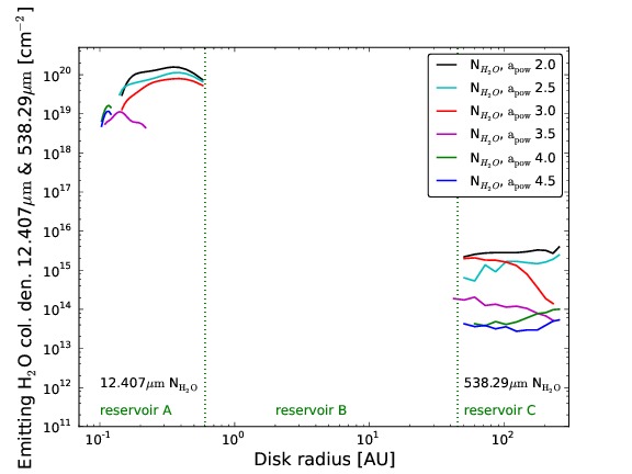
(b)

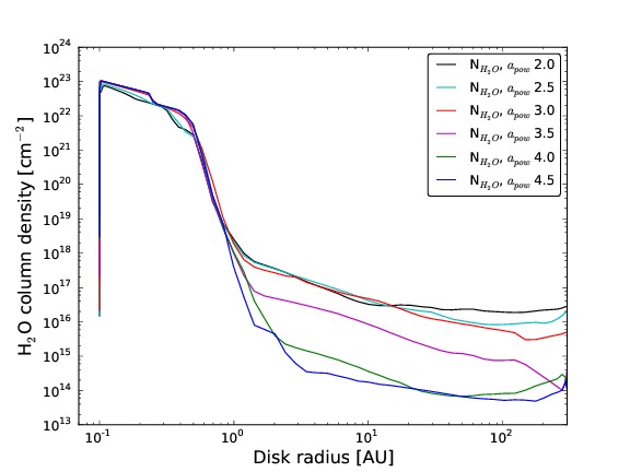
(c)

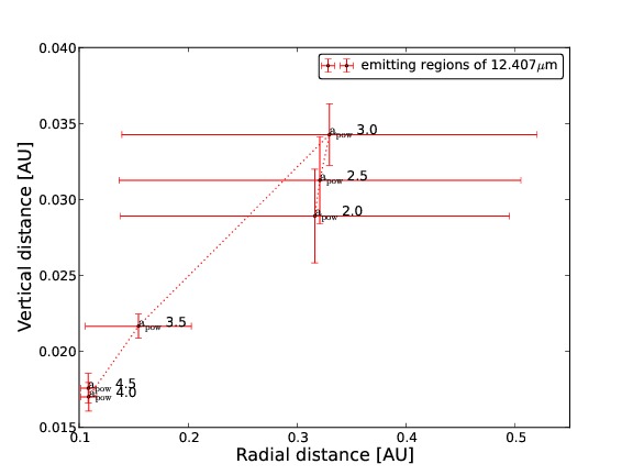
(d)

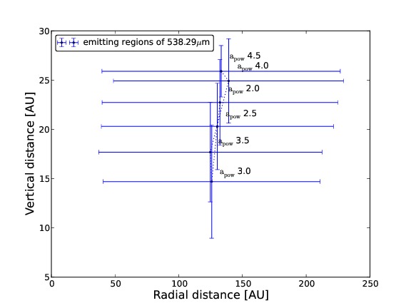
(e)

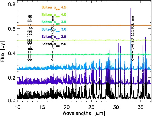
(f)

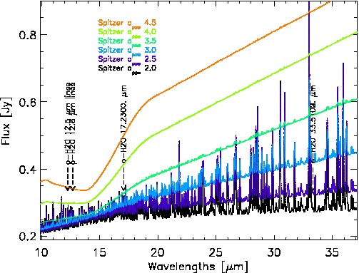
(g)

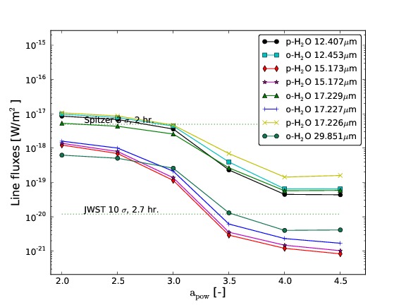
(h)

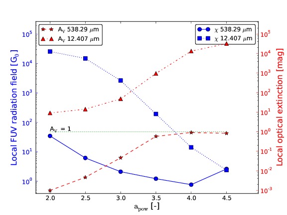
Figure 8: Plots for dust size distribution power law index models. For further details, see Fig. 4.

The modeled Spitzer spectrum (Fig. 8e & f) shows an increase of the continuum in the near-IR to mid-IR range and a lower line-to-continuum ratio for the models with a larger amount of small dust (high values of $a_{\mathrm{pow}}$). The mid-IR color variation is very high and the 13.5/30 $\mu$m continuum flux ratio decreases by more than a factor 2. The change in continuum flux is a consequence of settling (present in all the models). For larger $a_{\mathrm{pow}}$, the disk has more smaller grains (that are not settled), and so the warm surface layers contain a higher dust mass, which contributes to the continuum. In this case, the dust consists mainly of small grains and the opacity is high. As discussed in Sect. 4.1, the line-to-continuum ratio is then very low. The flat grain size distribution model has a lower opacity (flatter and more than 4 dex weaker in the UV-optical range), and the dust and gas temperature gradients are radially and vertically steeper than in the case of a steeper grain size distribution. Then, the dust becomes colder overall, producing less mid-IR continuum.

4.6 ISM radiation field

The ISM FUV radiation field affects the outer regions of the disk and changes the water column density beyond 30 AU in a complex way (Fig. 9b). In the most irradiated model, the total water column density decreases from photodissociation. In the emitting region of the Spitzer lines, the column density is unaffected below $\chi_{\mathrm{ISM}}\!=\!10^{3}\!\leavevmode\nobreak\ G_{\mathrm{0}}$ (Fig. 9a). The Spitzer line emitting region for $\chi_{\mathrm{ISM}}\!>\!10^{3}\!\leavevmode\nobreak\ G_{\mathrm{0}}$ extends over the entire disk, overlapping with the sub-mm lines. This happens because of a strong change in the thermal structure of the irradiated disk, and the formation of a hot layer of gas extending into the outer disk (beyond 10 AU). The hot gas extends down to the midplane for the $\chi_{\mathrm{ISM}}\!=\!10^{6}\!\leavevmode\nobreak\ G_{\mathrm{0}}$ model. Water is then eroded through photodissociation in the outer disk and the line is produced at smaller radii and closer to the midplane (Fig. 9d). The increase in $T_{\mathrm{gas}}$ for the more irradiated models ($\chi_{\mathrm{ISM}}\!>\!10^{3}\!\leavevmode\nobreak\ G_{\mathrm{0}}$) makes the line emitting regions radially more extended, and the mid-IR line fluxes increase (Fig. 9g).

In the outer disk, the opacity in the emitting region of the far-IR lines drops of an order of magnitude at $\chi_{\mathrm{ISM}}\!=\!10^{4}\!\leavevmode\nobreak\ G_{0}$, but then it raises again for larger $\chi_{\mathrm{ISM}}$. This is because of a complex variation in the total water column density in the outer disk (Fig. 9b & a), which also affects the emitting region’s extension and position (Fig. 9c & d). The far-IR lines first moves outward and then above $\chi_{\mathrm{ISM}}\!=\!10^{3}\!\leavevmode\nobreak\ G_{\mathrm{0}}$ inward and closer to the midplane. The line optical depth drops below 1.0 for $\chi_{\mathrm{ISM}}\!>\!10^{3}\!\leavevmode\nobreak\ G_{0}$ (Fig. 9d). Increasing the FUV radiation field, the emitting column density becomes larger because of enhanced photodesorption (Fig. 9a). The emitting region, however, is radially less extended because of increasing photodissociation, which removes water from the outer disk and even partially depletes the ice reservoir (Fig. 9b). The gas temperature in the emitting region increases from less than 100 K to 500 K and decouples from the dust temperature for models with $\chi_{\mathrm{ISM}}\!>\!100\!\leavevmode\nobreak\ G_{\mathrm{0}}$. The interplay between the increased temperature, the larger column density and the decreasing emitting area in the outer disk limits the sub-mm line flux increase to an order of magnitude.

(a)

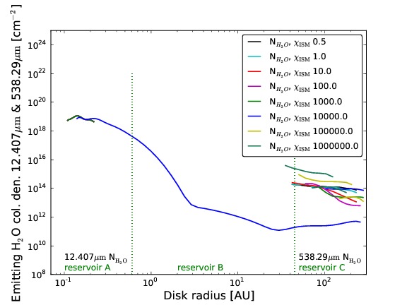
(b)

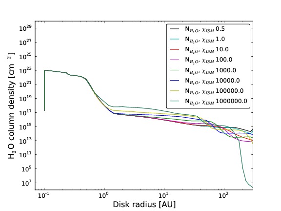
(c)

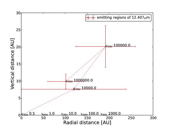
(d)

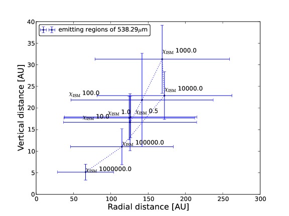
(e)

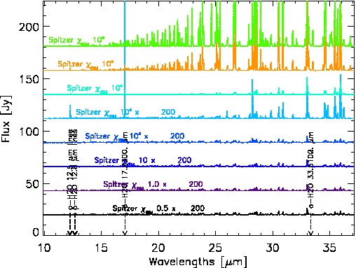
(f)

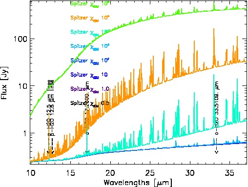
(g)

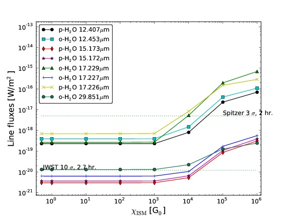
(h)

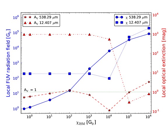
Figure 9: Plots for ISM radiation field models. For further details see Fig. 4.

The theoretical Spitzer spectrum (Fig. 9e & f) shows an increase of the line-to-continuum ratio for an increasing $\chi_{\mathrm{ISM}}$ up to 10 $G_{\mathrm{0}}$. For fluxes larger than 1000 $G_{\mathrm{0}}$, the continuum starts to become stronger, reducing the line-to-continuum ratio. This is due to the fact that $\chi_{\mathrm{ISM}}\!>\!\chi_{\mathrm{star}}$ ($\chi_{\mathrm{star}}\!\sim\leavevmode\nobreak\ \!10^{4}\!\leavevmode\nobreak\ G_{\mathrm{0}}$ within 2 AU). Beyond 10${}^{3}\!\leavevmode\nobreak\ G_{\mathrm{0}}$, the mid-IR color becomes much smaller than 1.

4.7 PAHs photoelectric heating

PAHs affect the total water column density by less than an order of magnitude in the outermost regions of the disk (Fig. 10a). The Spitzer transitions are almost unaffected (Fig. 10b). Their emitting region moves slightly upward and outward due to the increase in heating caused by PAHs (Fig. 10c). However, this displacement is too small to affect the line fluxes in the mid-IR. The column density in the emitting region of the far-IR lines increases by less than a factor of two with increasing $f_{\mathrm{PAH}}$. The sub-mm line emitting region moves outward and upward (Fig. 10d), but the gas temperature hardly changes. The line fluxes increase by a factor $\sim$ 2.

(a)

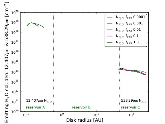
(b)

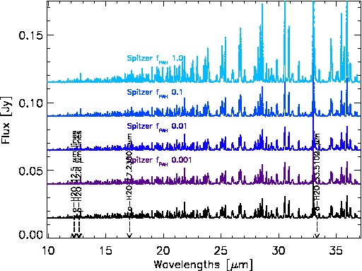
(c)

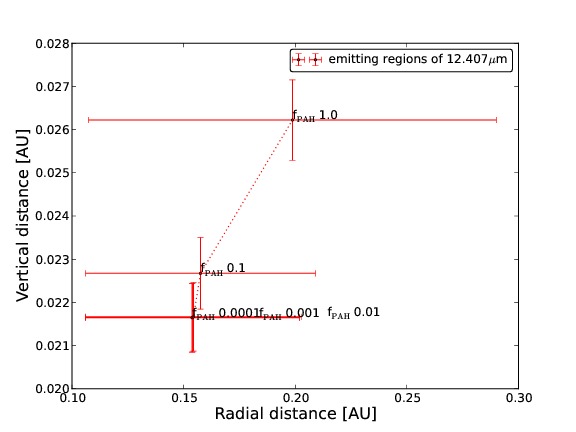
(d)

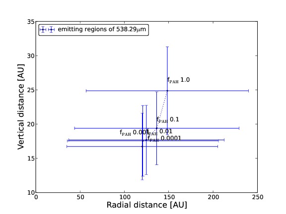
Figure 10: Plots for the fraction of PAHs models. (a) Emitting region water column density for dust-to-gas mass ratio models; this region comprises 15-85% of the radially and vertically integrated flux. Green vertical dotted lines distinguish the reservoirs. (b) Theoretical Spitzer SH/LH modules spectra ($R$ = 600) for a dust-to-gas model series, continuum subtracted, and arbitrarily shifted. (c) Average extension of the line emitting region, which comprises 50% of the line flux radially and vertically for 12.407 $\mu$m. (d) Average extension of the line emitting region, which comprises 50% of the line flux radially and vertically for 538.29 $\mu$m.

Since the dust opacities stay constant, the Spitzer spectra all show the same continuum; the 13.5/30 $\mu$m continuum flux ratio is thus also unaffected. The line-to-continuum ratio grows with increasing PAH abundance because of the heating effect on the gas.

4.8 Disk gas mass

The total gas mass in the disk affects almost proportionally the total water column density in the disk (Fig. 11b). All reservoirs are enhanced by the same amount with increasing gas mass. In the Spitzer emitting region, the gas density progressively increases for larger $M_{\mathrm{gas}}$. The water column density in the Spitzer water line emitting region follows a nonlinear trend (Fig. 11a). From $M_{\mathrm{gas}}$ 10^-5 to 10^-4 M_⊙, the emitting region moves outward and upward (Fig. 11c). Then, for masses larger than $M_{\mathrm{gas}}\!=\!10^{-4}\!\leavevmode\nobreak\ \mathrm{M_{\odot}}$, the migration of the line emitting region is inverted. Below a certain water column density ($N_{\mathrm{H_{2}O}}\!=\!1.6-8\cdot 10^{17}$ cm^-2, Bethell & Bergin, 2009), self-shielding becomes inefficient and water is strongly photodissociated. For the Spitzer line fluxes, the driving mechanism is first the increase of gas column density in the emitting region and, subsequently, the growth of the emitting region itself.

The water column density in the outer disk increases with $M_{\mathrm{gas}}$ (Fig. 11b) and also the optical depth of the lines. This causes the transition to be emitted progressively outward and higher up in the outer disk (Fig. 11d). Thus, the increase in the far-IR line flux with $M_{\mathrm{gas}}$ has the same explanation as the increase in the mid-IR lines.

(a)

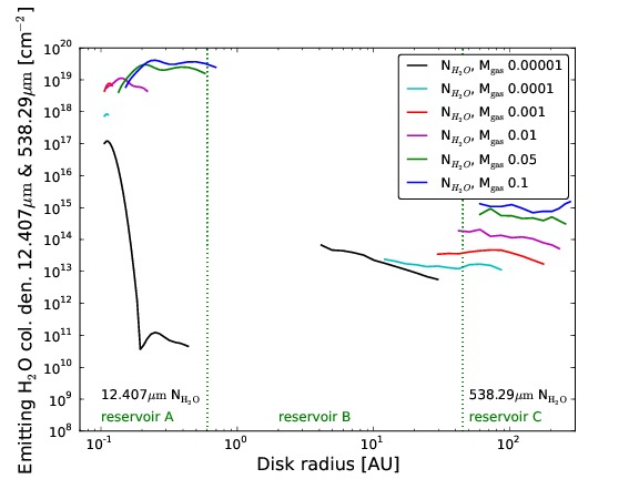
(b)

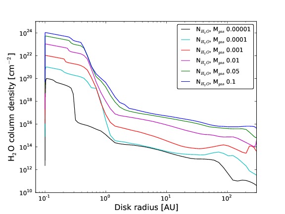
(c)

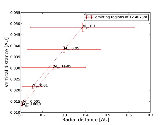
(d)

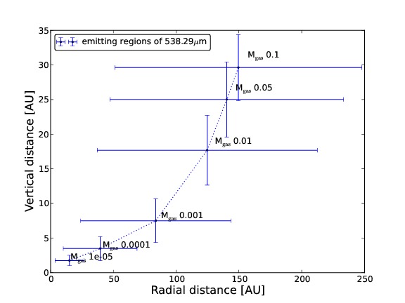
(e)

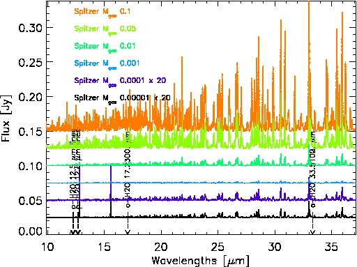
(f)

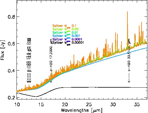
(g)

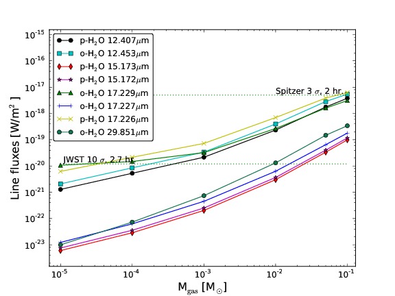
(h)

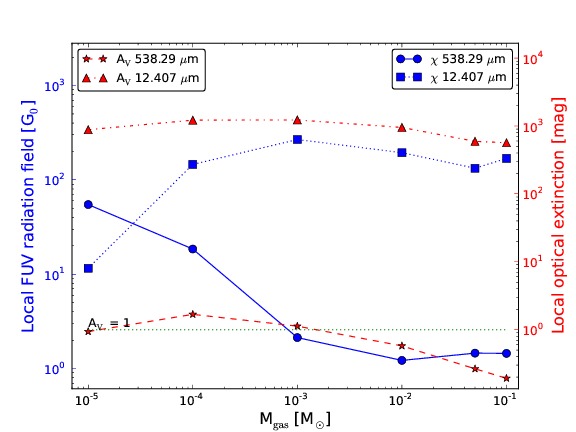
Figure 11: Plots for the gas mass content models. For further details see Fig. 4.

The theoretical Spitzer spectrum (Fig. 11e & f) cleary shows an increase in the line fluxes with the gas content of the disk. The different continuum level is a consequence of the dust settling. In the formalism adopted here, the corresponding dust scale height depends on the gas density, which is directly proportional to the mass of the gas in the disk. This means that increasing $M_{\mathrm{gas}}$ produces less settling, and hence a stronger IR continuum with a steeper slope. As a consequence, the mid-IR color becomes smaller.

5 Discussion

5.1 Discrimination between parameters affecting water line fluxes

The main goal of this work can be summarized in two questions:

1. Why do disks sometimes lack the detection of water?

2. Why are the water lines from the outer disk absent in disks that have clear detections of inner water reservoirs?

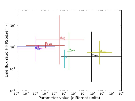
Figure 12: Overview of the line ratios Herschel/Spitzer (538.29 $\mu$m/12.407 $\mu$m) for all the parameters as a function of the explored range of values.

To answer these questions, we divide the parameters into three categories: those that strongly affect the line ratios (line flux variation $\geq$ 1 dex, parameter variation $<$ 1 dex); those that produce a relevant variation (line flux variation same order of magnitude as parameter variation); and parameters that produce a weak variation (line flux variation less than parameter variation). An overview of the effects of the parameters on continuum and line fluxes is listed in Table 8.

The Spitzer transitions around 12 $\mu$m are not those typically detected since their flux is weaker compared to other blends. We verified, however, that the same conclusions also hold for other mid-IR lines around 15, 17, and 29 $\mu$m. The conclusions about the far-IR lines are limited to the fundamental ortho and para water lines. The line forming regions of other far-IR lines suffer very large radial and vertical dispacements in these model series, hence, making the discussion even more complex. They will require a dedicated study.

The Herschel/HIFI lines would be largely undetectable with a standard observational setup and 1 hr of exposure, however, our modeling results suggest that the lines become detectable in many disks at a 5 $\sigma$ sensitivity level of 5$\cdot$10^-20 W/m². TW Hya required a total 181 min on-source integration with Herschel/HIFI to detect the 538.29 $\mu$m line (Hogerheijde et al., 2011).

In the first category, we find parameters such as the flaring index $\beta$ and the power law dust size distribution exponent $a_{\mathrm{pow}}$. These parameters are hard to constrain from observations of SEDs alone. The Herschel and Spitzer line fluxes are very sensitive to their exact values. Flaring affects the Herschel/HIFI lines strongly (2 dex) and the Spitzer transitions only marginally (less than a factor 3). The exponent of the dust grain size distribution produces larger changes in the Spitzer regime than in the Herschel regime. These flux variations are due to geometrical effects (in the outer disk, because of flaring, the emitting column of water and the area of the emitting region increase) and opacity/temperature changes (the inner disk in the flared models is directly exposed to the radiation, and so is warmer). In the case of the dust size distribution exponent, the far-IR is always emitted in an optically thin region, and therefore are less affected by any opacity change, while in the mid-IR regime the variation is about 4 dex and the line flux is suppressed. The external part (at larger radii) of reservoir B and all of reservoir C are optically thin in the continuum. This means that the line flux is directly affected by the variation in the dust opacity, and partially by a change in the local thermal conditions. For the transitions produced in the inner disk (as the Spitzer ones), the situation is driven by a change in the thermal structure since the lines are optically thick, with the exception o f very peculiar models explored in our series of models.

In the second category, we find almost all other parameters: dust-to-gas mass ratio, $d/g$; maximum dust size, $a_{\mathrm{max}}$; ISM radiation field, $\chi_{\mathrm{ISM}}$; and gas mass of the disk, $M_{\mathrm{gas}}$. Excluding the ISM radiation field, that is an environmental property, all the other properties are good candidates to understand the absence of a correlation between detections in the mid-IR and far-IR wavelength range. In these cases, the Spitzer lines are more affected by the parameter variations, and are strongly enhanced (3-4 dex) in disks with $M_{\mathrm{dust}}\!<\!10^{-4}\leavevmode\nobreak\ \!\leavevmode\nobreak\ M_{\mathrm{\odot}}$ and/or $M_{\mathrm{gas}}\!>$ 0.01 M_⊙, dust grains larger than 400 $\mu$m and few small grains ($a_{\mathrm{pow}}\!<$ 3.5). The continuum is enhanced in the presence of larger dust masses or smaller dust grains that absorb more FUV radiation and become warmer. Herschel lines show the same trend, but the magnitude of the variation is smaller. The effect of these parameters on the spectrum of the outer disk is not as important as in the inner disk.

The last category of parameters, mixing coefficient $\alpha_{\mathrm{set}}$ and fraction of polycyclic aromatic hydrocarbons $f_{\mathrm{PAH}}$, do not significantly affect the Spitzer nor the Herschel water emission lines. All water transitions respond in the same manner to the mixing coefficient. We stress here that the treatment of the mixing is disconnected from the viscous heating, which is set to zero in all our models. The PAHs are more important in the outer disk, which is optically thin, and is thus be warmed up by the increased photoelectric heating from PAHs. PAHs are not treated consistently as an opacity source, otherwise the enhanced opacity (expecially in the UV-optical regime) would have produced effects comparable to an increased dust-to-gas mass ratio in the disk.

Since every parameter affecting the line flux also modifies the emitting region position and extension in the disk, the line profiles are consequently affected, and outward displacements of the emitting regions produce narrower transitions (Keplerian velocity decreases with radial distances).

Our work finds that the main driver of water spectroscopy in the mid- to far-IR wavelengths range is the continuum opacity. Changes occur because of differences in the disk dust content or the opacity function ($a_{\mathrm{max}}$, $a_{\mathrm{pow}}$ variation). These directly affect the line flux (extinction) or indirectly affect the local thermal conditions (temperature change). The second effect is the disk geometry. A flared disk geometry exposes more water to the central stellar radiation field. Hence the total column density is depleted in the outer disk because of photodissociation. An increase in the ISM FUV radiation field also produces a suppression of water in the outermost reservoir C.

As discussed in Section 3.2, the mid-IR water lines are in LTE, while the outer disk water lines are marginally in non-LTE. Hence the far-IR line fluxes can be affected by uncertanties in the collision cross sections, as discussed in Kamp et al. (2013). We perform a sensitivity check on the standard model making a random variation (increase/decrease) of an order of magnitude in the water collisional constants. The results confirm the robustness of the conclusions presented in this paper: the line fluxes of the Spitzer transitions are unaffected, while the Herschel line variations are within 10%.

The disk water distribution found from the modeling is in qualitative agreement with recent modeling performed by Du & Bergin (2014). In particular, we reproduce the change of the column densities of water in the inner and outer disk due to the variation of dust-to-gas mass ratio and settling. A quantitative comparison is not possible because we use a more physical approach in our models (non-parametric settling; Dubrulle et al., 1995).

Table 7: General overview of the series of models results. All the variations refer to an increase of the respective parameter value.

Parameter∗	IRS lines	mid-IR continuum	HIFI lines	IRS line profiles	HIFI line profiles
$d/g$	$--$	$+$ (bolometrically)	$-$	narrower	unaffected
$\beta$	$+$	$+$ (bolometrically,	$++$	narrower	unaffected
$\alpha_{\mathrm{set}}$	$-$	$+$ (stronger with	$-$	unaffected	unaffected
$a_{\mathrm{max}}$	$++$	$-$	$+$	narrower	unaffected
$a_{\mathrm{pow}}$	$--$	$+$ (variation weaker	$-$	wider	unaffected
$\chi_{\mathrm{ISM}}$	$++$ (1)	$++$ (1)	$+$	narrower	unaffected
$f_{\mathrm{PAH}}$	x	x	$+$	unaffected	unaffected
$M_{\mathrm{gas}}$	$++$	$+$ (stronger with	$++$	narrower	narrower

5.2 Comparison with observations

Observationally, it will be difficult to assess the exact properties of a certain disk. Previous observational studies of mid-IR water spectroscopy used continuum diagnostics in the same spectral region to connect to disk properties of the targets. We expect to find such correlations, and we want to use them to define the position of each model produced by a parameter space exploration (that starts from our standard disk model), in a plot of the line flux vs. continuum flux. Here, we decide to use a mid-IR color (13.5/30; similar to what is used in Acke et al., 2009) because it traces slope changes in the Spitzer spectrum, and we found that that every parameter produces its own fingerprint. For the far-IR, we decided to use a diagnostic connected with the outer disk properties. We choose the SCUBA flux at 850 $\mu$m because it is available for many objects and traces dust mass to first order. We search for a direct relation between mid-IR colors, submm photometry, and simulated line fluxes at 12.407 $\mu$m and 538.29 $\mu$m. We distinguished three types of parameters (not to be confused with the categories defined in Sect. 5): parameters that change the dust opacity function ($a_{\mathrm{max}}$, $a_{\mathrm{pow}}$), parameters that change only the total opacity ($M_{\mathrm{gas}}$, $d/g$, $\alpha_{\mathrm{set}}$), and parameters that do not affect the opacity (ISM radiation field, $f_{\mathrm{PAH}}$, $\beta$). Every parameter produces its own signature on the SED and line fluxes, and Fig. 13 and Table 9 summarize the main findings. The parameter $M_{\mathrm{gas}}$ produces a limited variation in the mid-IR continuum, and a more important effect on the submm (82% in sub-mm, 10% in mid-IR, due to the settling). It produces a strong variation in the line flux both in the mid- and far-IR. Settling only modestly affects the line fluxes in both the regimes, but the mid-IR slope is strongly changed by up to 50% and the submm continuum flux changes by 87%. The dust-to-gas mass ratio does not strongly affect the mid-IR continuum (about 25%); however it changes the submm flux by almost a factor 2. Flaring significantly affects both the mid-IR continuum (90% relative variation) and the submm (more than 95% between extreme models), but the Spitzer lines are hardly affected. The ISM FUV radiation flux produces a stronger change in the Spitzer lines compared to the Herschel/HIFI lines, and a steepening of the IR excess beyond 10 $\mu$m. For the far-IR lines, the flux grows with increasing FUV radiation field until a certain limit and then levels off. The fraction of PAHs does not affect the SED, since the PAH opacity is not taken into account in the continuum radiative transfer.

A comparison of the modeling results with observations toward T Tauri disks shows that our simplified model predictions define a parameter space that is in good agreement with a number of objects: AA Tau, DG Tau, RW Aur, DM Tau for the mid-IR spectral region (top plot of Fig. 13), DG Tau, DM Tau, and TW Hya for the far-IR spectral region (bottom plot of Fig. 13). These targets have spectral types and properties compatible with our central star, and are not heavily affected by the presence of companions, either because they are too faint (case of RW Aur A+B; White & Ghez, 2001) or because the members are widely separated (DG Tau A+B; Mundt & Fried, 1983). Appendix C describes how the 12.4 $\mu$m blend flux was extracted from Spitzer spectra for the above targets and how continuum errors were propagated; fluxes are listed in Table 10. Fig. 13 compares the model results with the observational data: line blends around 12.4 $\mu$m versus our mid-IR color and 538.29 $\mu$m versus the SCUBA 850 $\mu$m flux. Our model series does not pretend to describe the situation of each target, which is a complex interplay of properties, but the position of the targets agree nicely with our models and support the predictional power of mid- and far-IR observations. The direct comparison with the sensitivities of Spitzer/IRS and JWST/MIRI (or Herschel/HIFI for the far-IR plot) shows the discovery potential of these facilities.

Fig. 13 shows that it is not possible to build trends that clearly connect line fluxes with continuum properties because different parameters affect the relation between these two quantities in a different manner. Hence, it is logical to expect a large amount of scatter in observations. Previous observational work (e.g.,  Pontoppidan et al., 2010b) show several plots with scattered observations in the continuum properties or line vs continuum fluxes or even continuum versus continuum. Any individual parameter produces a complex displacement in each of these plots, and every disk can be a different combination of parameters.

5.3 The future with JWST

The low resolution of the IRS spectrograph ($R$ = 600) does not enable an investigation of the line profiles; the blends usually contain several transitions (Banzatti, 2013). The problem is particularly important when the line profiles deviate from Keplerian rotation because of other kinematical components caused by winds/outflows/jets (Baldovin-Saavedra et al., 2011, 2012). The future facility to study mid-IR water lines is the James Webb Space Telescope (Greenhouse et al., 2014). The larger mirror and higher spectral resolution of the MIRI spectrograph ($\diameter\leavevmode\nobreak\ =\leavevmode\nobreak\ 6.5\leavevmode\nobreak\$m, $R\leavevmode\nobreak\ \simeq$ 3000; Clampin, 2011) will overcome the technical limitations of IRS. Fig. 14 shows a comparison of the mid-IR spectrum of our standard model in the Spitzer/IRS range with the resolution of the IRS and MIRI spectrographs. The higher sensitivity and the spectral coverage (5-28.5 $\mu$m) similar to Spitzer IRS, will allow us to detect water lines in almost all the cases modeled in this study, within a 2.7 hr exposure (10 $\sigma$; Fig. 13). Fig. 14 also shows that JWST/MIRI can make a decomposition of line blends into individual lines feasible, allowing, possibly for the first time, a quantitative analysis of the physical conditions in their emitting region.

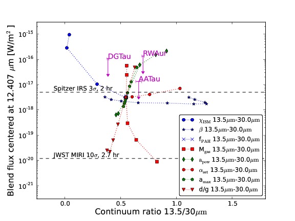
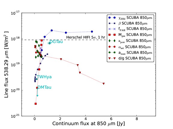
Figure 13: Line fluxes vs continuum. Top: 12.407 $\mu$m versus 13.5/30 IRS continuum flux ratios. Bottom: 538.29 $\mu$m versus the 850 $\mu$m SCUBA flux. Color code: blue for parameters not affecting the opacity, red for parameters affecting the total continuum opacity, green for parameters affecting the opacity function. Overplotted are the sensitivity limits for Spitzer/IRS, Herschel/HIFI, and JWST/MIRI (references in the text). The magenta data points are Spitzer/IRS observations available for stars with spectral type similar to our model central star, and blend fluxes have been extracted from Spitzer spectra following the procedure described in Appendix C. Cyan data points are the only Herschel/HIFI observations published for this submm line. All line fluxes have been scaled to 140 pc. Arrows indicate upper limits.

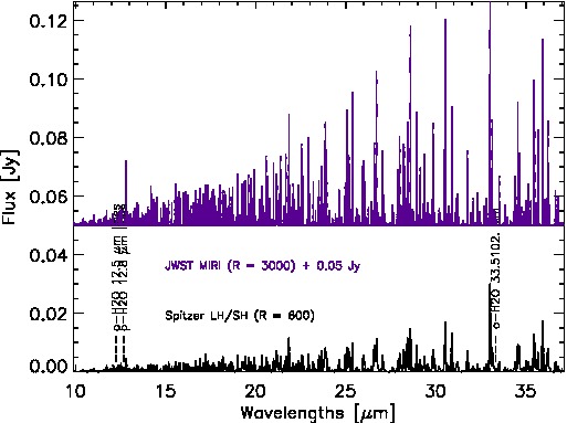
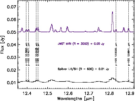
Figure 14: Mid-IR spectra of the standard disk model, continuum subtracted, convolved, and properly rebinned with the resolution of Spitzer/IRS LH/SH modules ($R$ = 600) and JWST/MIRI ($R$ = 3000) and arbitrarily shifted by 0.05 Jy. The bottom panel shows a zoom in the range 12.35-12.39 $\mu$m, JWST spectrum is again shifted by 0.05 Jy. The range of MIRI is artificially extended up to 37 $\mu$m to compare the performances.

Table 8: Line flux and color variation for the different parameters changes

Parameter	typea	Extreme ratiosb 538.29$\mu$m	Flux variation 850 $\mu$m [%]	Extreme ratiosb 12.407 $\mu$m	Flux ratio 13.5/30 variation
$a_{\mathrm{pow}}$	1	0.208	77.6	0.007	-0.453
amax	1	3.216	85.0	24.507	0.119
$M_{\mathrm{gas}}$	2	271.825	82.2	2600.789	-0.276
$d/g$	2	0.047	98.8	5.360	-0.253
$\alpha_{\mathrm{set}}$	2	0.456	87.5	0.454	-0.484
$\beta$	3	38.236	95.2	4.070	-0.911
$\chi_{\mathrm{ISM}}$	3	12.255	89.1	274.378	-0.532
$f_{\mathrm{PAH}}$	3	2.362	0.18	1.127	0.003

6 Conclusions

We explore here the parameter space around a standard T Tauri disk model to identify the main drivers of mid- and far-IR water spectroscopy. We primarly analyze two transitions, a mid-IR line at 12.407 $\mu$m and a far-IR line at 538.29 $\mu$m, representative of the whole group of transitions considered. In our series of models, we find that the gas mass and dust-to-gas mass ratio simultaneously affect water lines in the Spitzer and Herschel/HIFI wavelength ranges. Disks with a low gas content or high dust content are undetectable in both regimes. In the first case, the lack of emitting gas explains the nondetections, in the second case, the continuum opacity hides the water reservoirs. These two parameters could explain the occurrence of disks without any water features.

Dust properties ($a_{\mathrm{max}}$, $a_{\mathrm{pow}}$) only affect the mid-IR transitions, and can explain the nondetections of Spitzer lines, while the Herschel/HIFI transitions would be detectable in case of several hours of integration. On the other hand, flaring strongly affects the far-IR regime; so the nondetection of far-IR water lines can also be due to disk geometry.

Models with strong external FUV radiation field ($\chi_{\mathrm{ISM}}\!>\!10^{3}\!\leavevmode\nobreak\ G_{0}$) show strong mid-IR lines with narrow profiles. Herschel/HIFI lines are less affected and increase only by a factor of a few due to the external irradiation.

Our choice of implementing the PAHs only as a heating source and not as an opacity source causes the PAHs fraction to only weakly affect both mid- and far-IR lines. Our prescription of the settling is based on a physical description of the effects of gas vertical mixing on dust grains, but it is not related to the heating associated with the mechanical turbulence in the disk; the two phenomena are disconnected. In that case, the settling affects the inner disk physics very little.

We demonstrate the importance of future telescopes such as JWST in the investigation of water in disks. The higher sensitivity is capable of increasing dramatically the number of disks detected in water. The higher spectral resolution will permit us to detect unblended transitions, and to study in detail the physical conditions in the inner water reservoir.

Appendix A Computation of properties in the line emitting region

The different water lines are divided in groups based on their spatial origin. The latter is defined as that part of the disk from which a cumulative radially and vertically integrated flux of 15% to 85% of the total flux is produced. For each of these regions, averaged physical conditions $\left<X\right>$ are derived, such as the density of water, density of the collisional partners (e^-, H, H₂), $T_{\mathrm{gas}}$ and $T_{\mathrm{dust}}$ by numerically integrating over the emitting region (Eq. 5), i.e.,

$$\centering\left<X\right>=\frac{\int\limits_{r_{\mathrm{in}}}^{r_{\mathrm{out}}}\int\limits_{z_{\mathrm{low}}}^{z_{\mathrm{high}}}Xn_{\mathrm{gas}}2\pi rdrdz}{\int\limits_{r_{\mathrm{in}}}^{r_{\mathrm{out}}}\int\limits_{z_{\mathrm{low}}}^{z_{\mathrm{high}}}n_{\mathrm{gas}}2\pi rdrdz}\@add@centering$$ (5)

In order to determine the continuum extinction, a vertical integration is performed from the disk surface to the midplane. $\tau_{\nu}$ is the continuum optical depth at the frequency of the line. It is related to the dust density $\rho_{\mathrm{dust}}$ and dust mass extinction coefficient $\kappa_{\nu}$. The integration is performed numerically, as follows:

$$\centering\tau_{\nu}(z)=\int_{z_{\mathrm{max}}(r)}^{z(r,\tau_{\nu}=1)}\rho(r,z)\kappa_{\nu}dz\@add@centering$$ (6)

Through interpolation, we find the value at which $\tau_{\nu}$ = 1. The optical depth is evaluated at the radial midpoint of the emitting region.

Appendix B Model details

The following appendix shows a number of additional plots. These can be useful for the interpretation of the main results and conclusions reported in the paper.

Here we show the Herschel/HIFI fundamental o-H₂O and p-H₂O lines fluxes behavior with the different parameters.

Here, we also present plots collecting the main properties of the standard model: $T_{\mathrm{gas}}$, $T_{\mathrm{dust}}$, the local dust-to-gas mass ratio, local average dust size, and the main heating and cooling processes.

Line ratio plots are used to compare the relative behavior of the mid- and far-IR lines, considering two representative Spitzer water transitions and the Herschel fundamental ortho and para water lines. To show the trend clearly, we add a parabolic regression to the data (magenta lines).

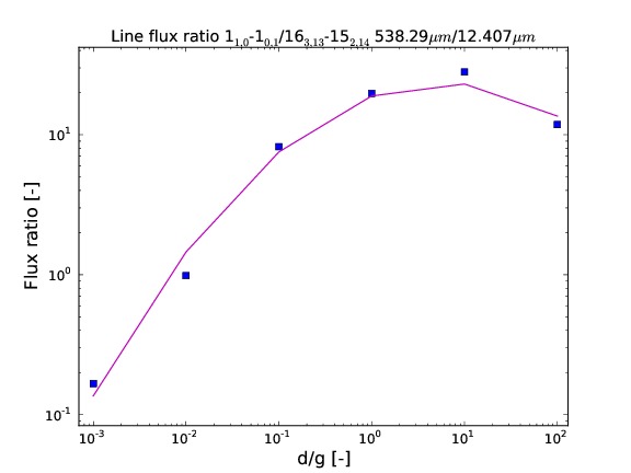
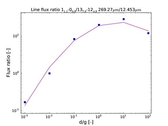
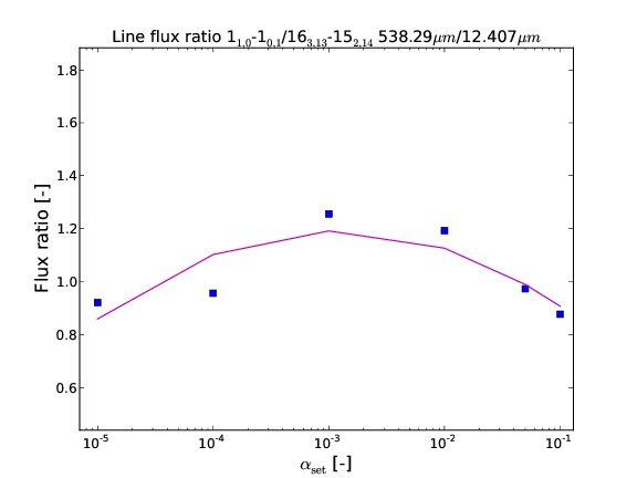
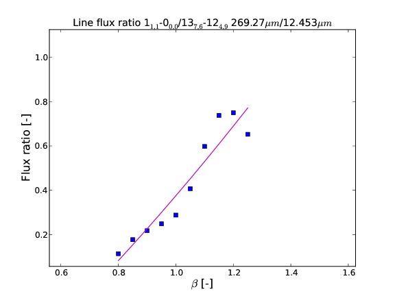
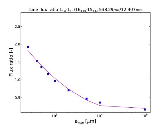
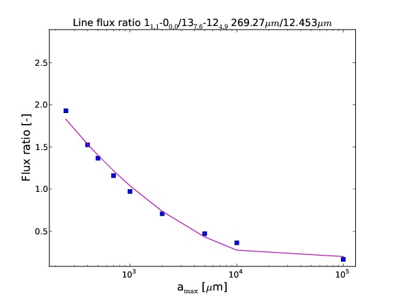
Figure 17: Ratios between Herschel/HIFI & Spitzer/IRS lines 538.29 $\rm\mu m$/12.407 $\rm\mu m$ and 269.27 $\rm\mu m$/12.453 $\rm\mu m$ for different model series. First row: dust-to-gas mass ratio, $d/g$. Second row: mixing parameter, $\alpha_{\mathrm{set}}$. Third row: disk flaring, $\beta$. Fourth row: maximum grain size, a_max.

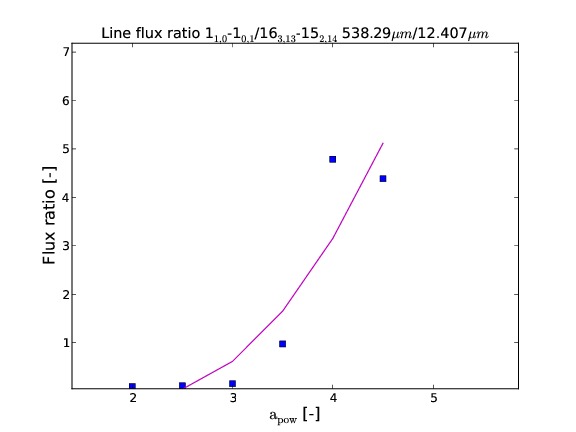
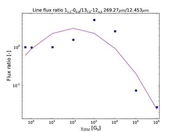
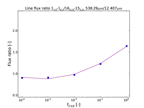
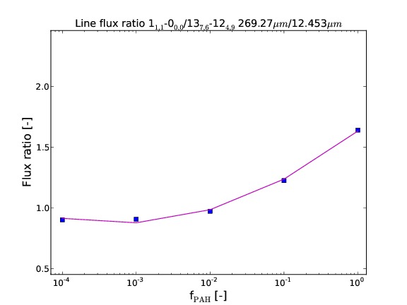
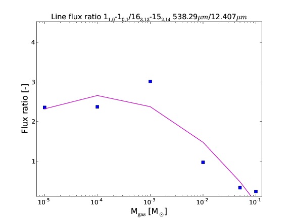
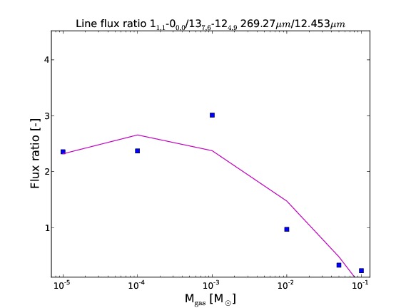
Fig. 17 Ratios between Herschel/HIFI & Spitzer/IRS lines 538.29 $\rm\mu m$/12.407 $\rm\mu m$ and 269.27 $\rm\mu m$/12.453 $\rm\mu m$ for different model series. Top: power law index of grain size distribution, $a_{\mathrm{pow}}$. Second line: strength of UV radiation field, $\chi_{\mathrm{ISM}}$. Third line: PAH abundance, $f_{\mathrm{PAH}}$. Fourth: disk gas mass, $M_{\mathrm{gas}}$.

Appendix C Mid- and far-IR observations

Table 9: Line and continuum observations of the targets discussed in the main paper.

Object	$d$ [pc]	$12.407\leavevmode\nobreak\ \mu$m blend flux∗∗	$13.5/30\leavevmode\nobreak\ \mu$m continuum	$538.29\leavevmode\nobreak\ \mu$m line flux	$850\leavevmode\nobreak\ \mu$m continuum(5)
		[10-17 W/m2]	flux ratio(1)	[10-20 W/m2]	[Jy]
AA Tau	140	$<$1.33	0.663$\pm$0.027	n.a.	n.a.
DM Tau	140	n.a.	n.a.	$<$1.15(4)	0.237$\pm$0.012
DG Tau	140	$<$10.63	0.388$\pm$0.008	67.00$\pm$7.00(2)	1.180$\pm$0.118
RW Aur	144	$<$13.51∗	0.702$\pm$0.010∗	n.a.	n.a.
TW Hya	56	n.a.	n.a.	2.72$\pm$0.12(3)∗	0.182$\pm$0.018∗

Far-IR line fluxes have been obtained from the literature. Mid-IR blends have been extracted from IRS spectra fitting a Gaussian function plus a linear continuum, computing the error in the flux as noise of the continuum,

$$F(\lambda)=A\times e^{(\lambda-\lambda_{0})^{2}/(2\sigma)^{2}}+B\times\lambda+C$$ (7)

This procedure is formally identical to that used in (Pontoppidan et al. 2010b). Table 10 lists all the observational data shown in Fig. 13 with respective references.

The mid-IR color 13.5/30 continuum flux is defined as pure ratio between the Spitzer/IRS fluxes at 13.5 $\mu$m and 30 $\mu$m, similarly to what is done in Acke et al. (2009) for the 30/13.5 continuum ratio. The observations overplotted include the errors propagated accordingly to

$$\sigma_{\mathrm{ratio}}=\frac{F_{13.5}}{F_{30}}\cdot\sqrt{\left(\frac{\sigma_{13.5}}{F_{13.5}}\right)^{2}+\left(\frac{\sigma_{30}}{F_{30}}\right)^{2}}$$ (8)