Self-Consistent Sources for Integrable Equations
via Deformations of Binary Darboux Transformations

Abstract

We reveal the origin and structure of self-consistent source extensions of integrable equations from the perspective of binary Darboux transformations. They arise via a deformation of the potential that is central in this method. As examples, we obtain in particular matrix versions of self-consistent source extensions of the KdV, Boussinesq, sine-Gordon, nonlinear Schrödinger, KP, Davey-Stewartson, two-dimensional Toda lattice and discrete KP equation. We also recover a (2+1)-dimensional version of the Yajima-Oikawa system from a deformation of the pKP hierarchy. By construction, these systems are accompanied by a hetero binary Darboux transformation, which generates solutions of such a system from a solution of the source-free system and additionally solutions of an associated linear system and its adjoint. The essence of all this is encoded in universal equations in the framework of bidifferential calculus.

1 Introduction

The study of soliton equations with self-consistent sources has been pursued in particular in the work of Mel’nikov [1, 2, 3, 4, 5, 6]. Mathematically, such systems of equations arise via a multiscaling limit of familiar integrable systems (see, e.g., [7, 5]), or via a symmetry constraint imposed on a higher than two-dimensional integrable system (see [8, 9], and also, e.g., [10, 11, 12, 13] for related work). Several of these systems appeared, independently from those more mathematical explorations, in various physical contexts. For example, the nonlinear Schrödinger (NLS) equation with self-consistent sources describes the nonlinear interaction of an electrostatic high-frequency wave with the ion acoustic wave in a plasma (cold ions, warm electrons) in a small amplitude limit [14, 15]. In nonlinear optics it describes the interaction of self-induced transparency and NLS solitons [16, 17]. By now quite a number of publications have been devoted to such equations.

In this work, we show that self-consistent source extensions arise via a simple deformation of the “potential” that appears in the binary Darboux transformation method (see, e.g., [18]). Moreover, the present work provides a more universal approach to such extensions, generalizations to matrix versions of such equations, and a corresponding solution generating method. This is achieved in the framework of bidifferential calculus [19, 20, 21].

In Section 2 we consider the example of the potential KP (pKP) equation with self-consistent sources. The underlying structure is then abstracted to bidifferential calculus in Section 3. The resulting system allows to generate self-consistent source extensions of other integrable equations and supplies them with a solution-generating method. Examples are treated in the further sections. In Appendix Appendix A: The extended matrix pKP hierarchy, we apply the aforementioned deformation to the matrix pKP hierarchy. The first non-trivial member then turns out to be a (2+1)-dimensional version [1] of the Yajima-Oikawa system [22]. Finally, Section 11 contains some concluding remarks.

2 Via binary Darboux transformation to self-consistent source extensions of the pKP equation

Let $\phi_{0}$ solve the matrix potential KP (pKP) equation, i.e.,

$$\left(4\,\phi_{0,t}-\phi_{0,xxx}-6\,(\phi_{0,x})^{2}\right)_{x}-3\,\phi_{0,yy}+6\,[\phi_{0,x},\phi_{0,y}]=0\,,$$ (2.1)

where a subscript $x,y$ or $t$ indicates a partial derivative with respect to this variable. A comma is used to separate them from subscripts of a different kind. Let $\theta,\eta$ solve the associated linear system and its adjoint, i.e.,

$$\theta_{y}=\theta_{xx}+2\,\phi_{0,x}\,\theta\,,\qquad\theta_{t}=\theta_{xxx}+3\,\phi_{0,x}\,\theta_{x}+\frac{3}{2}\left(\phi_{0,y}+\phi_{0,xx}\right)\,\theta$$ (2.2)

and

$$\eta_{y}=-\eta_{xx}-2\,\eta\,\phi_{0,x}\,,\qquad\eta_{t}=\eta_{xxx}+3\,\eta_{x}\,\phi_{0,x}-\frac{3}{2}\,\eta\,\left(\phi_{0,y}-\phi_{0,xx}\right)\,.$$ (2.3)

Both pairs of equations have the above pKP equation as consistency condition. As a consequence of these equations, the compatibility conditions of the system

$$\Omega_{x}=-\eta\,\theta\,,\qquad\Omega_{y}=-\eta\,\theta_{x}+\eta_{x}\,\theta\,,\qquad\Omega_{t}=-\eta\,\theta_{xx}+\eta_{x}\,\theta_{x}-\eta_{xx}\,\theta-3\,\eta\,\phi_{0,x}\,\theta\,,$$

are satisfied, which guarantees the existence of a “potential” $\Omega$. Then it follows that

$$\phi=\phi_{0}-\theta\,\Omega^{-1}\,\eta$$ (2.4)

is a new solution of (2.1), and

$$q=\theta\,\Omega^{-1}\,,\qquad r=\Omega^{-1}\,\eta\,,$$ (2.5)

solve (2.2) and (2.3), respectively, with $\phi$ instead of $\phi_{0}$. This is an essential step of the binary Darboux transformation method for the pKP equation.

Remark 2.1.

An attempt to iterate this procedure by using $\phi$, $q$ and $r$ instead of $\phi_{0}$, $\theta$ and $\eta$, leads back to the $\phi_{0}$ we started with to generate $\phi$. Iteration of the binary Darboux transformation method involves the construction of still other solutions of the linear systems. But we will not need these further steps here, since we consider a vectorial binary Darboux transformation, so that there is no need for iteration.

Let us now deform the potential $\Omega$ as follows,

$$\Omega_{x} = -\eta\,\theta+c_{1}\,,$$

$$\Omega_{y} = -\eta\,\theta_{x}+\eta_{x}\,\theta+c_{2}\,,$$

$$\Omega_{t} = -\eta\,\theta_{xx}+\eta_{x}\,\theta_{x}-\eta_{xx}\,\theta-3\,\eta\,\phi_{0,x}\,\theta+c_{3}\,,$$ (2.6)

with (matrix) functions $c_{i}$, $i=1,2,3$. Consistency requires that

$$c_{1}=\omega_{x}\,,\qquad c_{2}=\omega_{y}\,,\qquad c_{3}=\omega_{t}\,,$$

with a potential $\omega$. Hence the above deformation actually amounts to the substitution $\Omega\mapsto\Omega-\omega$ in the previous equations. Then $\phi,q,r$ no longer satisfy (2.1), (2.2) and (2.3). Instead we find

$$q_{y}-q_{xx} = 2\,\phi_{x}\,q+\left(-q\,\omega_{y}+q\,\omega_{xx}+2\,q_{x}\,\omega_{x}\right)\,\Omega^{-1}\,,$$

$$q_{t}-q_{xxx} = 3\,\phi_{x}\,q_{x}+\frac{3}{2}\left(\phi_{y}+\phi_{xx}\right)\,q+\frac{3}{2}\,\left(-q\,\omega_{y}+q\,\omega_{xx}+2\,q_{x}\,\omega_{x}\right)\,r\,q$$ (2.7)

$$+\left(-q\,\omega_{t}+q\,\omega_{xxx}+3\,(q_{x}\,\omega_{x})_{x}+3\,\phi_{x}\,q\,\omega_{x}\right)\,\Omega^{-1}\,,$$

$$r_{y}+r_{xx} = -2\,r\,\phi_{x}-\Omega^{-1}\left(\omega_{y}\,r+\omega_{xx}\,r+2\,\omega_{x}\,r_{x}\right)\,,$$

$$r_{t}-r_{xxx} = 3\,r_{x}\,\phi_{x}-\frac{3}{2}\,r\,\left(\phi_{y}-\phi_{xx}\right)+\frac{3}{2}\,r\,q\,\left(\omega_{y}\,r+\omega_{xx}\,r+2\,\omega_{x}\,r_{x}\right)$$ (2.8)

$$+\Omega^{-1}\,\left(-\omega_{t}\,r+\omega_{xxx}\,r+3\,(\omega_{x}\,r_{x})_{x}+3\,\omega_{x}\,r\,\phi_{x}\right)\,,$$

and the extended pKP equation

$$\left(4\,\phi_{t}-\phi_{xxx}-6\,(\phi_{x})^{2}\right)_{x}-3\,\phi_{yy}+6\,[\phi_{x},\phi_{y}]$$ (2.9)

$$= \left(4\,q\,\omega_{t}\,r-6\,q\,\omega_{x}\,r_{y}-6\,q\,\omega_{x}\,r_{xx}+6\,q\,\omega_{y}\,r_{x}-18\,q\,\omega_{xx}\,r_{x}-6\,q\,\omega_{xy}\,r-10\,q\,\omega_{xxx}\,r\right)_{x}$$

$$+\left(6\,q\,\omega_{x}\,r_{x}-3\,q\,\omega_{y}\,r+9\,q\,\omega_{xx}\,r\right)_{y}+\left(6\,q\,\omega_{x}\,r_{x}-3\,q\,\omega_{y}\,r+9\,q\,\omega_{xx}\,r\right)_{xx}\,.$$

If $\phi$ is an $m\times m$ matrix, then $\theta,q$ have matrix size $m\times n$, and $\eta,r$ have size $n\times m$. $\Omega$ and $\omega$ are then $n\times n$ matrices.

Remark 2.2.

Using (2.5), and introducing $\hat{\Omega}:=-\Omega^{-1}$, we turn (2.6) into the Riccati system

$$\hat{\Omega}_{x}=-r\,q+\hat{\Omega}\,\omega_{x}\,\hat{\Omega}\,,\qquad\hat{\Omega}_{y}=-r\,q_{x}+r_{x}\,q+\hat{\Omega}\,\omega_{y}\,\hat{\Omega}\,,$$

$$\hat{\Omega}_{t}=-r\,q_{xx}+r_{x}\,q_{x}-r_{xx}\,q-3\,r\,\phi_{x}\,q+\hat{\Omega}\,\omega_{t}\,\hat{\Omega}\,.$$

This completes the system consisting of (2.7), (2.8) (where $\Omega^{-1}$ should be replaced by $-\hat{\Omega}$) and (2.9). The above hetero binary Darboux transformation can now be inverted to map solutions of (2.7), (2.8) and (2.9) to solutions of the source-free pKP equation and solutions of its linear system:

$$\phi_{0}=\phi-q\,\hat{\Omega}^{-1}r\,,\quad\theta=-q\,\hat{\Omega}^{-1}\,,\quad\eta=-\hat{\Omega}^{-1}\,r\,.$$

The equations for $q,r$ and $\hat{\Omega}$ are nonlinear, however, and thus more difficult to solve.

Next we look for choices of $\omega$, such that $\Omega$ can be eliminated in half of the equations (2.7) and (2.8). This requires $\omega_{x}=0$ and leaves us with the choices $\omega_{y}=0$ or $\omega_{t}=0$. In the first case, we only keep the equations for $q_{y}$ and $r_{y}$. In the second case, we only keep those for $q_{t}$ and $r_{t}$. This results in the two versions of pKP with self-consistent sources that appeared in the literature.

1. $\omega=\omega(t)$.

   $$\left(4\,\phi_{t}-\phi_{xxx}-6\,(\phi_{x})^{2}\right)_{x}-3\,\phi_{yy}+6\,[\phi_{x},\phi_{y}]=4\,\left(q\,\omega_{t}\,r\right)_{x}\,,$$

   $$q_{y}-q_{xx}=2\,\phi_{x}\,q\,,\qquad r_{y}+r_{xx}=-2\,r\,\phi_{x}\,.$$ (2.10)

   In terms of

   $$\tilde{q}=q\,\mathcal{Q}\,,\qquad\tilde{r}=\mathcal{R}\,r\,,$$ (2.11)

   with a suitable choice of $\mathcal{Q}(t)$ and $\mathcal{R}(t)$, this system can be written as

   $$\left(4\,\phi_{t}-\phi_{xxx}-6\,(\phi_{x})^{2}\right)_{x}-3\,\phi_{yy}+6\,[\phi_{x},\phi_{y}]=(\tilde{q}\,\tilde{r})_{x}\,,$$

   $$\tilde{q}_{y}-\tilde{q}_{xx}=2\,\phi_{x}\,\tilde{q}\,,\qquad\tilde{r}_{y}+\tilde{r}_{xx}=-2\,\tilde{r}\,\phi_{x}\,,$$ (2.12)

   where $\omega_{t}$ has been absorbed. The latter is rather what we should call a system with self-consistent sources. Its scalar version has been studied in [1, 23, 4, 7, 24, 25, 26, 27]. The “noncommutative” generalization (2.12) already appeared in [28]. In our framework, the modification (2.10) is important. By actually solving (2.10), we obtain solutions of the self-consistent source system (2.12), which depend on arbitrary functions of $t$. The appearance of arbitrary functions of a single variable in solutions is a generic feature of systems with self-consistent sources.

2. $\omega=\omega(y)$.

   $$\left(4\,\phi_{t}-\phi_{xxx}-6\,(\phi_{x})^{2}\right)_{x}-3\,\phi_{yy}+6\,[\phi_{x},\phi_{y}]=3\,\left(q\,\omega_{y}\,r_{x}-q_{x}\,\omega_{y}\,r\right)_{x}-3\,\left(q\,\omega_{y}\,r\right)_{y}\,,\qquad\quad$$

   $$q_{t}-q_{xxx}=3\,\phi_{x}\,q_{x}+\frac{3}{2}\left(\phi_{y}+\phi_{xx}\right)\,q-\frac{3}{2}\,q\,\omega_{y}\,r\,q\,,$$

   $$r_{t}-r_{xxx}=3\,r_{x}\,\phi_{x}-\frac{3}{2}\,r\,\left(\phi_{y}-\phi_{xx}\right)+\frac{3}{2}\,r\,q\,\omega_{y}\,r\,.$$ (2.13)

   Again, introducing new variables as in (2.11), now with a suitable $\mathcal{Q}(y)$ and $\mathcal{R}(y)$, $\omega_{y}$ can be absorbed. The scalar version of this system has been studied in [1, 26].

Remark 2.3.

In the scalar case ($m=1$), if $\omega$ does not depend on $x$, the expression (2.4) can be rewritten as $\phi=\phi_{0}+\mathrm{tr}(-\theta\,\Omega^{-1}\,\eta)=\phi_{0}+\mathrm{tr}(\Omega_{x}\,\Omega^{-1})=\phi_{0}+(\ln(\det\Omega))_{x}$. Together with (2.5), this provides us with solutions of the scalar versions of (2.7) and (2.8). If $\omega$ depends only on $t$ or $y$, we obtain solutions of (2.10) and (2.13), respectively.

Remark 2.4.

As formulated above, the number of sources appears to be $n$. However, this is only so if $\omega_{t}$, respectively $\omega_{y}$, has maximal rank. If the rank is $N<n$, then only $N$ sources appear on the right hand side of (2.9).

The above procedure provides us with a hetero binary Darboux transformation from the pKP equation and its associated linear system to any of the pKP systems with self-consistent sources (modified by $\omega$). In the framework of bidifferential calculus, we can abstract the underlying structure from the specific example (here pKP) and then obtain corresponding self-consistent source extensions of quite a number of other integrable equations.

Remark 2.2 shows that there is also a transformation that maps a class of solutions of any of the self-consistent source extensions of the pKP equation to solutions of the source-free pKP equation and its linear system. We expect that this is a general feature of integrable systems with self-consistent sources.

Exact solutions in case of constant seed.

Let $\phi_{0}$ be constant. Special solutions of (2.2) and (2.3) are given by

$$\theta=a\,e^{\vartheta(P)}\,A\,,\qquad\eta=B\,e^{-\vartheta(Q)}\,b\,,\qquad\vartheta(P):=P\,x+P^{2}\,y+P^{3}\,t\,,$$

with constant matrices $a$, $b$, $A$, $B$, $P$ and $Q$ of appropriate size. Then (2.6) is solved by

$$\Omega=\omega-B\,e^{-\vartheta(Q)}\,X\,e^{\vartheta(P)}\,A\,,$$

with a constant matrix $X$ that satisfies the Sylvester equation

$$X\,P-Q\,X=b\,a\,.$$

(2.4) and (2.5) now provide us with explicit solutions of the above matrix pKP equations with self-consistent sources, (2.10) and (2.13). The basic soliton solutions are obtained if $P$ and $Q$ are diagonal with distinct eigenvalues, and if they have disjoint spectra, in which case the Sylvester equation has a unique solution. Also see [29] for the source-free case.

Example 2.5.

In the scalar case ($m=1$), choosing $n=1$, $a=A=B=b=1$ and $\omega=e^{\alpha}/(Q-P)$, where $\alpha$ is either a function only of $y$ or of $t$, we obtain

$$\phi=\phi_{0}+\frac{(P-Q)\,e^{{\vartheta(P)}-\vartheta(Q)}}{e^{\alpha}+e^{{\vartheta(P)}-\vartheta(Q)}}=\phi_{0}+\frac{1}{2}(P-Q)+\left(\ln(\cosh\Theta)\right)_{x}\,,$$

$$q=\frac{(Q-P)\,e^{{\vartheta(P)}}}{e^{\alpha}+e^{{\vartheta(P)}-\vartheta(Q)}}=\frac{1}{2}(Q-P)\,e^{\tilde{\Theta}}\,\mathrm{sech}(\Theta)\,,\;r=\frac{(Q-P)\,e^{-{\vartheta(Q)}}}{e^{\alpha}+e^{{\vartheta(P)}-\vartheta(Q)}}=\frac{1}{2}(Q-P)\,e^{-\tilde{\Theta}-\alpha}\,\mathrm{sech}(\Theta),$$

where $\Theta=\frac{1}{2}\left(\vartheta(P)-\vartheta(Q)-\alpha\right)$ and $\tilde{\Theta}=\frac{1}{2}\left(\vartheta(P)+\vartheta(Q)-\alpha\right)$. Then $u=\phi_{x}$, together with $q$ and $r$, or rather the transformed $\tilde{q}$ and $\tilde{r}$, is a soliton solution of the scalar KP equation with self-consistent sources. Also see [30, 24, 25, 31].

3 A framework for generating self-consistent source extensions of integrable equations

Let us recall some basics of bidifferential calculus. A graded associative algebra is an associative algebra $\boldsymbol{\Omega}=\bigoplus_{r\geq 0}\boldsymbol{\Omega}^{r}$ over $\mathbb{C}$, where $\mathcal{A}:=\boldsymbol{\Omega}^{0}$ is an associative algebra over $\mathbb{C}$ and $\boldsymbol{\Omega}^{r}$, $r\geq 1$, are $\mathcal{A}$-bimodules such that $\boldsymbol{\Omega}^{r}\,\boldsymbol{\Omega}^{s}\subseteq\boldsymbol{\Omega}^{r+s}$. A bidifferential calculus is a unital graded associative algebra $\boldsymbol{\Omega}$, supplied with two ($\mathbb{C}$-linear) graded derivations $\mathrm{d},\bar{\mathrm{d}}:\boldsymbol{\Omega}\rightarrow\boldsymbol{\Omega}$ of degree one (hence $\mathrm{d}\boldsymbol{\Omega}^{r}\subseteq\boldsymbol{\Omega}^{r+1}$, $\bar{\mathrm{d}}\boldsymbol{\Omega}^{r}\subseteq\boldsymbol{\Omega}^{r+1}$), and such that

$$\mathrm{d}^{2}=\bar{\mathrm{d}}^{2}=\mathrm{d}\bar{\mathrm{d}}+\bar{\mathrm{d}}\mathrm{d}=0\,.$$ (3.1)

In this framework, many integrable equations can be expressed either as

$$\mathrm{d}\,\bar{\mathrm{d}}\,\phi_{0}+\mathrm{d}\phi_{0}\;\mathrm{d}\phi_{0}=0\,,$$ (3.2)

with $\phi_{0}\in\mathrm{Mat}(m,m,\mathcal{A})$ (the algebra of $m\times m$ matrices over $\mathcal{A}$), and possibly with some reduction condition, or as

$$\mathrm{d}\,[(\bar{\mathrm{d}}g_{0})\,g_{0}^{-1}]=0\,,$$ (3.3)

with an invertible $g_{0}\in\mathrm{Mat}(m,m,\mathcal{A})$. The two equations are related by the Miura equation

$$\bar{\mathrm{d}}g_{0}=(\mathrm{d}\phi_{0})\,g_{0},$$ (3.4)

which has both, (3.2) and (3.3), as integrability conditions. (3.2) and (3.3) are generalizations or analogs of well-known potential forms of the self-dual Yang-Mills equation (cf. [20]).

A linear system and an adjoint linear system for (3.2) is given by

$$\bar{\mathrm{d}}\theta=(\mathrm{d}\phi_{0})\,\theta+(\mathrm{d}\theta)\,\Delta+\theta\,\lambda\,,$$ (3.5)

respectively

$$\bar{\mathrm{d}}\eta=-\eta\,\mathrm{d}\phi_{0}+\Gamma\,\mathrm{d}\eta+\kappa\,\eta\,,$$ (3.6)

where $\theta\in\mathrm{Mat}(m,n,\mathcal{A})$, $\eta\in\mathrm{Mat}(n,m,\mathcal{A})$, $\Delta,\Gamma\in\mathrm{Mat}(n,n,\mathcal{A})$, and $\lambda,\kappa$ are $n\times n$ matrices of elements of $\Omega^{1}$. They have to satisfy

$$\bar{\mathrm{d}}\Delta+[\lambda,\Delta]=(\mathrm{d}\Delta)\,\Delta\,,\qquad\bar{\mathrm{d}}\lambda+\lambda^{2}=(\mathrm{d}\lambda)\,\Delta\,,$$

$$\bar{\mathrm{d}}\Gamma-[\kappa,\Gamma]=\Gamma\,\mathrm{d}\Gamma\,,\qquad\bar{\mathrm{d}}\kappa-\kappa^{2}=\Gamma\,\mathrm{d}\kappa\,,$$ (3.7)

as a consequence of (3.1) and the graded derivation property of $\mathrm{d}$ and $\bar{\mathrm{d}}$.

Binary Darboux transformation.

Let $\Omega$ be a solution of

$$\Gamma\,\Omega-\Omega\,\Delta=\eta\,\theta\,,$$ (3.8)

$$\bar{\mathrm{d}}\Omega=(\mathrm{d}\Omega)\,\Delta-(\mathrm{d}\Gamma)\,\Omega+\kappa\,\Omega+\Omega\,\lambda+(\mathrm{d}\eta)\,\theta\,.$$ (3.9)

The equation obtained by acting with $\bar{\mathrm{d}}$ on (3.8) is identically satisfied as a consequence of (3.5), (3.6), (3.8), and the equation that results from (3.8) by acting with $\mathrm{d}$ on it. Correspondingly, also the equation that results from acting with $\bar{\mathrm{d}}$ on (3.9) is identically satisfied as a consequence of the preceding equations. It follows [20] that

$$\phi=\phi_{0}-\theta\,\Omega^{-1}\,\eta$$

is a new solution of (3.2), and

$$q=\theta\,\Omega^{-1}\,,\qquad r=\Omega^{-1}\,\eta\,,$$

satisfy

$$\bar{\mathrm{d}}q=(\mathrm{d}\phi)\,q+\mathrm{d}(q\,\Gamma)-q\,\kappa\,,\qquad\bar{\mathrm{d}}r=-r\,(\mathrm{d}\phi)+\mathrm{d}(\Delta\,r)-\lambda\,r\,.$$

Deformation of the potential.

Guided by the pKP example in the preceding section, we replace $\Omega$ by $\Omega-\omega$ in the above equations, i.e.,

$$\Gamma\,(\Omega-\omega)-(\Omega-\omega)\,\Delta=\eta\,\theta\,,$$

$$\bar{\mathrm{d}}(\Omega-\omega)=\mathrm{d}(\Omega-\omega)\,\Delta-(\mathrm{d}\Gamma)\,(\Omega-\omega)+\kappa\,(\Omega-\omega)+(\Omega-\omega)\,\lambda+(\mathrm{d}\eta)\,\theta\,.$$

Hence

$$\Gamma\,\Omega-\Omega\,\Delta=\eta\,\theta+c\,,$$

$$\bar{\mathrm{d}}\Omega=(\mathrm{d}\Omega)\,\Delta-(\mathrm{d}\Gamma)\,\Omega+\kappa\,\Omega+\Omega\,\lambda+(\mathrm{d}\eta)\,\theta+\gamma\,,$$ (3.10)

where

$$c:=\Gamma\,\omega-\omega\,\Delta\,,\qquad\gamma:=\bar{\mathrm{d}}\omega-(\mathrm{d}\omega)\,\Delta+(\mathrm{d}\Gamma)\,\omega-\kappa\,\omega-\omega\,\lambda\,.$$ (3.11)

We note that they satisfy

$$\bar{\mathrm{d}}\gamma=(\mathrm{d}\gamma)\,\Delta-(\mathrm{d}\Gamma)\,\gamma+\kappa\,\gamma-\gamma\,\lambda-(\mathrm{d}\kappa)\,c\,,$$

$$\bar{\mathrm{d}}c=(\mathrm{d}c)\,\Delta+\kappa\,c+c\,\lambda+\Gamma\,\gamma-\gamma\,\Delta\,.$$ (3.12)

By straightforward computations, one proves the following.

Theorem 3.1.

Let $\phi_{0}$ be a solution of (3.2) and let $\theta$, $\eta$, $\Omega$ satisfy the linear equations (3.5), (3.6) and (3.10), respectively. Then

$$\phi=\phi_{0}-\theta\,\Omega^{-1}\,\eta\,,\qquad q=\theta\,\Omega^{-1}\,,\qquad r=\Omega^{-1}\,\eta\,,$$ (3.13)

are solutions of

$$\mathrm{d}\,\bar{\mathrm{d}}\,\phi+\mathrm{d}\phi\;\mathrm{d}\phi=\mathrm{d}(q\,\gamma\,r-q\,\mathrm{d}(c\,r))$$ (3.14)

and

$$\bar{\mathrm{d}}q = (\mathrm{d}\phi)\,q+\mathrm{d}(q\,\Gamma)-q\,\kappa-q\,\gamma\,\Omega^{-1}-(\mathrm{d}q)\,c\,\Omega^{-1}\,,$$

$$\bar{\mathrm{d}}r = -r\,\mathrm{d}\phi+\mathrm{d}(\Delta\,r)-\lambda\,r-\Omega^{-1}\,\gamma\,r+\Omega^{-1}\,\mathrm{d}(c\,r)\,.$$ (3.15)

From (3.14) and (3.15) we can recover the self-consistent source extensions of the pKP equation, revisited in the preceding section, see below. But now we can choose different bidifferential calculi and obtain self-consistent source extensions also of other integrable equations. A number of examples will be presented in the following sections. In all these examples, we have $c=0$, i.e.,

$$\Gamma\,\omega=\omega\,\Delta\,.$$ (3.16)

Remark 3.2.

The above equations form a consistent system in the sense that any equation derived from it by acting with $\bar{\mathrm{d}}$ on any of its members yields an equation that is satisfied as a consequence of the system.

Remark 3.3.

Using the last two equations in (3.13), we eliminate $\theta$ and $\eta$ in (3.10) to obtain

$$\Delta\,\hat{\Omega}-\hat{\Omega}\,\Gamma=r\,q+\hat{\Omega}\,c\,\hat{\Omega}\,,$$

$$\bar{\mathrm{d}}\hat{\Omega}=\mathrm{d}(\hat{\Omega}\Gamma)-\hat{\Omega}\,\kappa-\lambda\,\hat{\Omega}+(\mathrm{d}r)\,q+\left((\mathrm{d}\hat{\Omega})\,c+\hat{\Omega}\,\gamma\right)\,\hat{\Omega}\,,$$

where $\hat{\Omega}=-\Omega^{-1}$. (3.15) then reads

$$\bar{\mathrm{d}}q = (\mathrm{d}\phi)\,q+\mathrm{d}(q\,\Gamma)-q\,\kappa+q\,\gamma\,\hat{\Omega}+(\mathrm{d}q)\,c\,\hat{\Omega}\,,$$

$$\bar{\mathrm{d}}r = -r\,\mathrm{d}\phi+\mathrm{d}(\Delta\,r)-\lambda\,r+\hat{\Omega}\,\gamma\,r-\hat{\Omega}\,\mathrm{d}(c\,r)\,.$$

Together with (3.14), this constitutes a system of equations for $\phi$, $q$, $r$ and $\hat{\Omega}$, for which we now have a solution-generating technique at hand. Also see Remark 2.2.

Generating solutions of the equations for $g$.

If $\phi_{0}$ and $g_{0}$ satisfy the Miura equation (3.4), then $\phi,q,r$ together with

$$g=(I-\theta\,\Omega^{-1}\,\Gamma^{-1}\eta)\,g_{0}\,,$$

where $I$ is the identity matrix, satisfy

$$\bar{\mathrm{d}}g-(\mathrm{d}\phi)\,g=(q\,\gamma+(\mathrm{d}q)\,c)\,\Omega^{-1}\,\Gamma^{-1}\,\Omega\,r\,g_{0}\,.$$

If (3.16) holds, i.e., $c=0$, then we have

$$g^{-1}=g_{0}^{-1}\,(I+\theta\,\Delta^{-1}\,\Omega^{-1}\,\eta)\,,$$

and $g$ satisfies the extended Miura equation

$$\bar{\mathrm{d}}g-(\mathrm{d}\phi)\,g=(q\,\gamma\,\Delta^{-1}\,r)\,g\,,$$ (3.17)

which implies the following extension of (3.3),

$$\mathrm{d}[(\bar{\mathrm{d}}g)\,g^{-1}]=\mathrm{d}(q\,\gamma\,\Delta^{-1}\,r)\,.$$ (3.18)

Via the extended Miura equation (3.17), we can eliminate $\phi$ in (3.15) in favor of $g$. The resulting equations, together with (3.18), constitute the (Miura-) dual of (3.14) and (3.15). It is another generating system for further self-consistent source extensions of integrable equations.

Transformations.

The equations for $\Delta$ and $\lambda$ in (3.7) and the linear equation (3.5) are invariant under a transformation

$$\theta\mapsto\theta\,L\,,\quad\Delta\mapsto L^{-1}\,\Delta\,L\,,\quad\lambda\mapsto L^{-1}\,\lambda\,L+L^{-1}\,\bar{\mathrm{d}}L+(\mathrm{d}L^{-1})\,\Delta\,L\,,$$

with an invertible $L$. Correspondingly, the equations for $\Gamma$ and $\kappa$ in (3.7) and the linear equation (3.6) are invariant under

$$\eta\mapsto M\,\eta\,,\quad\Gamma\mapsto M\,\Gamma\,M^{-1}\,,\quad\kappa\mapsto M\,\kappa\,M^{-1}+(\bar{\mathrm{d}}M)\,M^{-1}+M\,\Gamma\,\mathrm{d}M^{-1}\,,$$

with an invertible $M$. (3.10) is invariant if we supplement these transformations by $\Omega\mapsto M\,\Omega\,L$ and $\omega\mapsto M\,\omega\,L$. Now (3.12) implies $c\mapsto M\,c\,L$ and $\gamma\mapsto M\,\gamma\,L$. The formula for $\phi$ in (3.13) is invariant, and those for $q$ and $r$ imply $q\mapsto q\,M^{-1}$ and $r\mapsto L^{-1}\,r$. It follows that (3.14), (3.15), (3.16), (3.17) and (3.18) are invariant. This suggests that, via such a transformation, $\kappa$ and $\lambda$ can typically be eliminated. However, Sections 4-7 show that this may not necessarily be so and that special choices of $\kappa$ and $\lambda$ can achieve a drastic simplification of the equations.

Choice of the graded algebra.

In this work, we specify the graded algebra $\boldsymbol{\Omega}$ to be of the form

$$\boldsymbol{\Omega}=\mathcal{A}\otimes\boldsymbol{\Lambda}\,,\qquad\boldsymbol{\Lambda}=\bigoplus_{i=0}^{2}\boldsymbol{\Lambda}^{i}$$ (3.19)

where $\boldsymbol{\Lambda}$ is the exterior (Grassmann) algebra of the vector space $\mathbb{C}^{2}$. It is then sufficient to define $\mathrm{d}$ and $\bar{\mathrm{d}}$ on $\mathcal{A}$, since they extend to $\boldsymbol{\Omega}$ in a straightforward way, treating the elements of $\boldsymbol{\Lambda}$ as constants. Moreover, $\mathrm{d}$ and $\bar{\mathrm{d}}$ extend to matrices over $\boldsymbol{\Omega}$. We choose a basis $\xi_{1},\xi_{2}$ of $\boldsymbol{\Lambda}^{1}$.

Recovering the pKP case.

Let $\mathcal{A}_{0}$ be the space of smooth complex functions on $\mathbb{R}^{3}$. We extend it to $\mathcal{A}=\mathcal{A}_{0}[\partial]$, where $\partial:=\partial_{x}$ is the partial differentiation operator with respect to $x$. On $\mathcal{A}$ we define (cf. [20])

$$\mathrm{d}f=[\partial,f]\,\xi_{1}+\frac{1}{2}\,[\partial_{y}+\partial^{2},f]\,\xi_{2}\,,\qquad\bar{\mathrm{d}}f=\frac{1}{2}\,[\partial_{y}-\partial^{2},f]\,\xi_{1}+\frac{1}{3}\,[\partial_{t}-\partial^{3},f]\,\xi_{2}\,.$$

The maps $\mathrm{d}$ and $\bar{\mathrm{d}}$ extend to linear maps on $\boldsymbol{\Omega}=\mathcal{A}\otimes\boldsymbol{\Lambda}$, and moreover to matrices over $\boldsymbol{\Omega}$. Choosing

$$\Delta=\Gamma=-I_{n}\partial\,,\qquad\kappa=\lambda=0\,,$$

where $I_{n}$ is the $n\times n$ identity matrix, (3.7) is satisfied, and $c=0$, i.e., (3.16), becomes $\omega_{x}=0$. The second equation in (3.11) leads to

$$\gamma=\frac{1}{2}\omega_{y}\,\xi_{1}+\left(\frac{1}{3}\omega_{t}+\frac{1}{2}\omega_{y}\,\partial\right)\,\xi_{2}\,.$$

(3.10) becomes (2.6) with $c_{1}=0$, $c_{2}=\omega_{y}$, $c_{3}=\omega_{t}$. Taking $\omega_{x}=0$ into account, we recover all equations in Section 2. For example, (3.15) yields (2.7) and (2.8), and (3.14) becomes (2.9). A corresponding extension of the whole pKP hierarchy is presented in Appendix Appendix A: The extended matrix pKP hierarchy.

4 Matrix KdV equation with self-consistent sources

Let $\mathcal{A}_{0}$ be the space of smooth complex functions on $\mathbb{R}^{2}$. We extend it to $\mathcal{A}=\mathcal{A}_{0}[\partial]$, where $\partial:=\partial_{x}$ is the partial differentiation operator with respect to the coordinate $x$. On $\mathcal{A}$ we define (cf. [20])

$$\mathrm{d}f=[\partial,f]\,\xi_{1}+\frac{1}{2}\,[\partial^{2},f]\,\xi_{2}\,,\qquad\bar{\mathrm{d}}f=-\frac{1}{2}\,[\partial^{2},f]\,\xi_{1}+\frac{1}{3}\,[\partial_{t}-\partial^{3},f]\,\xi_{2}\,.$$

The maps $\mathrm{d}$ and $\bar{\mathrm{d}}$ extend to linear maps on $\boldsymbol{\Omega}=\mathcal{A}\otimes\boldsymbol{\Lambda}$, and moreover to matrices over $\boldsymbol{\Omega}$. Choosing

$$\Delta=\Gamma=-I_{n}\partial\,,\quad\kappa=\frac{1}{2}\,Q^{2}\,(\xi_{1}+\partial\,\xi_{2})\,,\quad\lambda=-\frac{1}{2}\,P^{2}\,(\xi_{1}+\partial\,\xi_{2})\,,$$

with constant matrices $P,Q$, (3.7) is satisfied, and (3.16) becomes $\omega_{x}=0$. The choices for $\kappa$ and $\lambda$ considerably simplify the subsequent equations. The second equation in (3.11) yields

$$\gamma=\gamma_{1}\,\xi_{1}+(\gamma_{2}+\gamma_{1}\,\partial)\,\xi_{2}\,,\qquad\gamma_{1}=-\frac{1}{2}(Q^{2}\omega-\omega\,P^{2})\,,\quad\gamma_{2}=\frac{1}{3}\,\omega_{t}\,.$$

The linear equations (3.5) and (3.6) read

$$\theta_{xx}=\theta\,P^{2}-2\,\phi_{0,x}\,\theta\,,\quad\theta_{t}=\theta_{x}\,P^{2}+\phi_{0,x}\,\theta_{x}-\frac{1}{2}\phi_{0,xx}\,\theta\,,$$

$$\eta_{xx}=Q^{2}\eta-2\eta\,\phi_{0,x}\,,\quad\eta_{t}=Q^{2}\eta_{x}+\eta_{x}\,\phi_{0,x}-\frac{1}{2}\eta\,\phi_{0,xx}\,,$$

and (3.10) takes the form

$$Q^{2}\,\Omega-\Omega\,P^{2}=\eta\,\theta_{x}-\eta_{x}\,\theta+Q^{2}\,\omega-\omega\,P^{2}\,,$$

$$\Omega_{x}=-\eta\,\theta\,,\quad\Omega_{t}=-Q^{2}\,\eta\,\theta-\eta\,\theta\,P^{2}+\eta_{x}\,\theta_{x}+\eta\,\phi_{0,x}\,\theta+\omega_{t}\,.$$ (4.1)

According to Section 3, it follows that $\phi$, $q$ and $r$, given by (3.13), satisfy

$$4\,u_{t}-u_{xxx}-3\,(u^{2})_{x}=8\,(q\,\omega_{t}\,r)_{x}+6\,\left(q_{x}\,(Q^{2}\omega-\omega P^{2})\,r-q\,(Q^{2}\omega-\omega P^{2})\,r_{x}\right)_{x}\,,$$

$$q_{xx}=q\,Q^{2}-u\,q-q\,(Q^{2}\,\omega-\omega P^{2})\,\Omega^{-1}\,,$$

$$q_{t}=q_{x}\,Q^{2}+\frac{1}{2}q\,(Q^{2}\omega-\omega\,P^{2})\,r\,q+\frac{1}{2}u\,q_{x}-\frac{1}{4}u_{x}\,q-q_{x}\,(Q^{2}\omega-\omega\,P^{2})\,\Omega^{-1}-q\,\omega_{t}\,\Omega^{-1}$$

$$\quad=q_{xxx}+\frac{3}{2}u\,q_{x}+\frac{3}{4}u_{x}\,q+\frac{3}{2}q\,(Q^{2}\omega-\omega\,P^{2})\,r\,q-q\,\omega_{t}\,\Omega^{-1}\,,$$

$$r_{xx}=P^{2}\,r-r\,u+\Omega^{-1}\,(Q^{2}\omega-\omega\,P^{2})\,,$$

$$r_{t}=P^{2}\,r_{x}-\frac{1}{2}r\,q\,(Q^{2}\omega-\omega\,P^{2})\,r+\frac{1}{2}r_{x}\,u-\frac{1}{4}r\,u_{x}+\Omega^{-1}\,(Q^{2}\omega-\omega\,P^{2})\,r_{x}-\Omega^{-1}\,\omega_{t}\,r$$

$$\quad=r_{xxx}+\frac{3}{2}r_{x}\,u+\frac{3}{4}r\,u_{x}-\frac{3}{2}r\,q\,(Q^{2}\omega-\omega\,P^{2})\,r-\Omega^{-1}\,\omega_{t}\,r\,,\qquad$$ (4.2)

where we introduced $u=2\,\phi_{x}$. From this we obtain the following two versions of a matrix KdV equation with self-consistent sources.

1. Setting $\gamma_{1}=0$, i.e.,

   $$Q^{2}\omega=\omega\,P^{2}\,,$$ (4.3)

   and disregarding the equations for $q_{t}$ and $r_{t}$, (4.2) reduces to

   $$4\,u_{t}-u_{xxx}-3\,(u^{2})_{x}=8\,(q\,\omega_{t}\,r)_{x}\,,\quad q_{xx}=q\,Q^{2}-u\,q\,,\quad r_{xx}=P^{2}\,r-r\,u\,.$$ (4.4)

   Here $\omega_{t}$ can be absorbed by a redefinition of either $q$ or $r$, which exchanges $P$ and $Q$ in the corresponding linear equation due to a necessary application of (4.3). The scalar version appeared in [3], also see [33, 34, 35, 36].

2. $\gamma_{2}=0$, i.e., constant $\omega$. In this case (4.2) yields

   $$4\,u_{t}-u_{xxx}-3\,(u^{2})_{x}=\left(\tilde{q}_{x}\,r-\tilde{q}\,r_{x}\right)_{x}\,,$$

   $$\tilde{q}_{t}=\tilde{q}_{xxx}+\frac{3}{2}\,u\,\tilde{q}_{x}+\frac{3}{4}u_{x}\,\tilde{q}+\frac{3}{2}\tilde{q}\,r\,\tilde{q}\,,\quad r_{t}=r_{xxx}+\frac{3}{2}\,r_{x}\,u+\frac{3}{4}r\,u_{x}-\frac{3}{2}r\,\tilde{q}\,r\,,\qquad$$ (4.5)

   where we introduced $\tilde{q}=6\,q\,(Q^{2}\omega-\omega P^{2})$. This system is also obtained from (2.13) by assuming that $\phi,q,r$ do not depend on $y$, whereas $\omega_{y}$ is non-zero, but constant. We note that (4.5) is a system of evolution equations for all dependent variables. In this respect it is very different from all other examples of systems with self-consistent sources presented in this work, with the exception of (5.1).

Exact solutions for vanishing seed.

Let $\phi_{0}$ be constant, i.e., $u_{0}=0$. Then we have the following solutions of the linear equations,

$$\theta=a_{1}\,e^{\vartheta(P)}+a_{2}\,e^{-\vartheta(P)}\,,\quad\eta=e^{\vartheta(Q)}\,b_{1}+e^{-\vartheta(Q)}\,b_{2}\,,\quad\vartheta(P)=P\,x+P^{3}\,t\,,$$ (4.6)

with constant matrices $a_{i},b_{i}$. A corresponding solution of (4.1) is

$$\Omega=e^{\vartheta(Q)}\,A_{11}\,e^{\vartheta(P)}+e^{-\vartheta(Q)}\,A_{22}\,e^{-\vartheta(P)}+e^{-\vartheta(Q)}\,A_{21}\,e^{\vartheta(P)}+e^{\vartheta(Q)}\,A_{12}\,e^{-\vartheta(P)}+\omega\,,$$

with constant matrices $A_{ij}$ that satisfy the Sylvester equations

$$QA_{11}+A_{11}P=-b_{1}a_{1}\,,\quad QA_{22}+A_{22}P=b_{2}a_{2}\,,\quad QA_{21}-A_{21}P=b_{2}a_{1}\,,\quad QA_{12}-A_{12}P=-b_{1}a_{2}\,.$$

Then (3.13) yields exact solutions of (4.4), respectively (4.5), under the corresponding condition for $\omega$.

Example 4.1.

In case of the first version of a KdV equation with self-consistent sources, for the sake of definiteness we choose $\omega(t)=\beta(t)\,I_{n}$. Then (4.3) leads to $Q=\pm P$. The two cases turn out to be equivalent, hence we choose $Q=P$. Now (3.13) determines a class of exact solutions of (4.4). Fig. 1 shows an example of a modulated 2-soliton solution. Introducing $\tilde{r}=\beta\,r$, this becomes a solution of (4.4) without the presence of $\omega_{t}$.

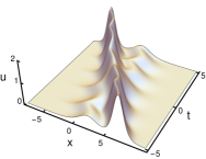
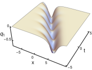
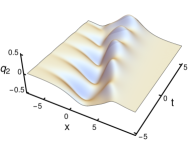
Figure 1: Plots of a 2-soliton solution of the first scalar KdV equation with self-consistent sources, see Example 4.1. Here we chose $\beta(t)=\sin(3t)$, $p_{1}=1$, $p_{2}=-1/2$, $a_{1}=b_{1}^{\intercal}=(1,0)$ and $a_{2}=(0,1)=b_{2}^{\intercal}$ in (4.6). The plots for $r_{1}$ and $r_{2}$ look like those for $q_{1}$ and $q_{2}$.

Example 4.2.

In case of the second KdV equation with self-consistent sources, let $n=1$. Then we obtain the following 2-soliton solution of (4.5),

$$\phi=\frac{2\,(P^{2}-Q^{2})}{D}\,\cosh(\vartheta_{1})\,\sinh(\vartheta_{2})\,,\quad\tilde{q}=\frac{e^{-\nu_{1}-\nu_{2}}\,(P+Q)\,(Q^{2}\omega-\omega P^{2})}{D}\,\cosh(\vartheta_{1})\,,$$

$$r=\frac{e^{-\mu_{1}-\mu_{2}}\,(P-Q)}{D}\,\sinh(\vartheta_{2})\,,\quad D:=\omega+(Q-P)\,\cosh(\vartheta_{1}+\vartheta_{2})+(Q+P)\,\cosh(\vartheta_{1}-\vartheta_{2})\,,$$

with constants $\mu_{i},\nu_{i}$ and $\vartheta_{1}=\vartheta(P)+\mu_{1}-\mu_{2}$, $\vartheta_{2}=\vartheta(Q)+\nu_{1}-\nu_{2}$.

5 Matrix Boussinesq equation with self-consistent sources

Let $\mathcal{A}_{0}$ be the space of smooth complex functions on $\mathbb{R}^{2}$, with coordinates $x$ and $t$, and $\mathcal{A}=\mathcal{A}_{0}[\partial]$, where $\partial:=\partial_{x}$ is the partial differentiation operator with respect to $x$. On $\mathcal{A}$ we define a bidifferential calculus via

$$\mathrm{d}f=[\partial,f]\,\xi_{1}+\frac{1}{2}\,[\partial_{t}+\partial^{2},f]\,\xi_{2}\,,\qquad\bar{\mathrm{d}}f=\frac{1}{2}\,[\partial_{t}-\partial^{2},f]\,\xi_{1}-\frac{1}{3}\,[\partial^{3},f]\,\xi_{2}\,.$$

Setting

$$\Delta=\Gamma=-I_{n}\partial\,,\quad\kappa=-\frac{1}{3}\,Q^{3}\,\xi_{2}\,,\quad\lambda=-\frac{1}{3}\,P^{3}\,\xi_{2}\,,$$

with constant matrices $P,Q$, (3.7) is satisfied, and (3.16) becomes $\omega_{x}=0$. The second equation in (3.11) yields

$$\gamma=\gamma_{1}\,\xi_{1}+(\gamma_{2}+\gamma_{1}\,\partial)\,\xi_{2}\,,\qquad\gamma_{1}=\frac{1}{2}\,\omega_{t}\,,\quad\gamma_{2}=\frac{1}{3}\,(Q^{3}\omega+\omega\,P^{3})\,.$$

The linear equations (3.5) and (3.6) read

$$\theta_{xxx}=\theta\,P^{3}-3\,\phi_{0,x}\,\theta_{x}-\frac{3}{2}(\phi_{0,t}+\phi_{0,xx})\,\theta\,,\qquad\theta_{t}=\theta_{xx}+2\,\phi_{0,x}\,\theta\,,$$

$$\eta_{xxx}=Q^{3}\eta-3\,\eta_{x}\,\phi_{0,x}+\frac{3}{2}\eta\,(\phi_{0,t}-\phi_{0,xx})\,,\qquad\eta_{t}=-\eta_{xx}-2\,\eta\,\phi_{0,x}\,,$$

and (3.10) takes the form

$$Q^{3}(\Omega-\omega)+(\Omega-\omega)\,P^{3}=-\eta\,\theta_{xx}+\eta_{x}\,\theta_{x}-\eta_{xx}\,\theta-3\,\eta\,\phi_{0,x}\,\theta\,,$$

$$\Omega_{x}=-\eta\,\theta\,,\qquad(\Omega-\omega)_{t}=-\eta\,\theta_{x}+\eta_{x}\,\theta\,.$$

Our general results in Section 3 imply that $\phi$, $q$ and $r$, given by (3.13), satisfy

$$3\,\phi_{tt}+\phi_{xxxx}+6\,(\phi_{x}{}^{2})_{x}-6\,[\phi_{x},\phi_{t}]=-\left(4\,q\,(Q^{3}\omega+\omega\,P^{3})\,r+3\,q\,\omega_{t}\,r_{x}-3\,q_{x}\omega_{t}\,r\right)_{x}+3\,(q\,\omega_{t}\,r)_{t}\,,$$

$$q_{xxx}=-q\,Q^{3}-3\,\phi_{x}q_{x}-\frac{3}{2}(\phi_{t}+\phi_{xx})\,q+\frac{3}{2}q\,\omega_{t}r\,q+q\,(Q^{3}\omega+\omega\,P^{3})\,\Omega^{-1}\,,$$

$$q_{t}=q_{xx}+2\,\phi_{x}q-q\,\omega_{t}\,\Omega^{-1}\,,$$

$$r_{xxx}=-P^{3}\,r-3\,r_{x}\,\phi_{x}+\frac{3}{2}r\,(\phi_{t}-\phi_{xx})-\frac{3}{2}r\,q\,\omega_{t}\,r+\Omega^{-1}\,(Q^{3}\omega+\omega\,P^{3})\,r\,,$$

$$r_{t}=-r_{xx}-2\,r\,\phi_{x}-\Omega^{-1}\,\omega_{t}\,r\,.$$

From this we obtain the following two versions of a matrix Boussinesq equation with self-consistent sources. Here we set $u:=2\phi_{x}$.

1. $Q^{3}\omega+\omega\,P^{3}=0$.

   $$3\,u_{tt}+u_{xxxx}+3\,(u^{2})_{xx}-3\,[u,\partial^{-1}u_{t}]_{x}=-6\,\left(q\,\omega_{t}\,r_{x}-q_{x}\omega_{t}\,r\right)_{xx}+6\,(q\,\omega_{t}\,r)_{xt}\,,$$

   $$q_{xxx}=-q\,Q^{3}-\frac{3}{2}\,u\,q_{x}-\frac{3}{4}(\partial^{-1}u_{t}+u_{x})\,q+\frac{3}{2}q\,\omega_{t}r\,q\,,$$

   $$r_{xxx}=-P^{3}\,r-\frac{3}{2}\,r_{x}\,u+\frac{3}{4}r\,(\partial^{-1}u_{t}-u_{x})-\frac{3}{2}r\,q\,\omega_{t}r\,.$$

   The scalar version appeared in [37].

2. $\omega_{t}=0$, i.e., constant $\omega$.

   $$3\,u_{tt}+u_{xxxx}+3\,(u^{2})_{xx}-3\,[u,\partial^{-1}u_{t}]_{x}=\left(\tilde{q}\,r\right)_{xx}\,,$$

   $$\tilde{q}_{t}=\tilde{q}_{xx}+u\,\tilde{q}\,,\qquad r_{t}=-r_{xx}-r\,u\,.$$ (5.1)

   where we introduced $\tilde{q}=-8\,q\,(Q^{3}\omega+\omega\,P^{3})$. In contrast to most systems with self-consistent sources obtained in this work, here we have evolution equations for all dependent variables. Also see (4.5).

Solutions with vanishing seed.

If $u_{0}=\phi_{0,x}/2=0$, solutions of the linear equations are given by

$$\theta=a_{0}\,e^{\vartheta(P)}+a_{1}\,e^{\vartheta(\zeta\,P)}+a_{2}\,e^{\vartheta(\zeta^{2}\,P)}\,,\qquad\eta=e^{-\vartheta(-Q)}\,b_{0}+e^{-\vartheta(-\zeta\,Q)}\,b_{1}+e^{-\vartheta(\zeta^{2}\,Q)}\,b_{2}\,,$$

where $a_{i},b_{i}$ are constant and

$$\zeta:=e^{2\pi\mathrm{i}/3}\,,\qquad\vartheta(P):=P\,x+P^{2}\,t\,.$$

A corresponding solution of the equations for $\Omega$ is then given by

$$\Omega=\sum_{j,k=0}^{2}e^{-\vartheta(-\zeta^{k}Q)}\,A_{kj}\,e^{\vartheta(\zeta^{j}P)}+\omega\,,$$

where $A_{kj}$ are constant matrices subject to

$$\zeta^{k}Q\,A_{kj}+\zeta^{j}A_{kj}\,P=-b_{k}\,a_{j}\qquad\quad j,k=0,1,2\,.$$

Now (3.13) yields exact solutions of the above Boussinesq systems with self-consistent sources. In case of the first version, we still have to take the constraint $Q^{3}\omega=-\omega\,P^{3}$ into account.

6 Matrix sine-Gordon equation with self-consistent sources

Let $\mathcal{A}_{0}$ be an associative algebra, where the elements depend on variables $x$ and $y$. Let $\mathcal{A}=\mathcal{A}_{0}[J]$, where $J$ is an idempotent operator that determines an involution ^∗ via $Jf=:f^{\ast}\,J$, for $f\in\mathcal{A}_{0}$, i.e., $f^{\ast}=JfJ$. A bidifferential calculus is then determined on $\mathcal{A}$ by setting

$$\mathrm{d}f=[\partial_{x},f]\,\xi_{1}+\frac{1}{2}[J,f]\,\xi_{2}\,,\qquad\bar{\mathrm{d}}f=\frac{1}{2}[J,f]\,\xi_{1}+[\partial_{y},f]\,\xi_{2}\,.$$

In order to eliminate explicit appearances of the operator $J$ in the equations resulting from the linear equations (3.5) and (3.6), we write

$$\phi=\varphi\,J\,,\quad\Delta=P\,J\,,\quad\Gamma=J\,Q\,,$$

$$\kappa=J\,(\kappa_{1}+\frac{1}{2}I)\,\xi_{1}+(\kappa_{2}-\frac{1}{2}Q^{\ast})\,\xi_{2}\,,\quad\lambda=(\lambda_{1}-\frac{1}{2}I)\,J\,\xi_{1}+(\lambda_{2}+\frac{1}{2}P^{\ast})\,\xi_{2}\,,$$

where $\varphi,P,Q,\kappa_{i},\lambda_{i}$ can now be taken to be matrices over $\mathcal{A}_{0}$. We will assume that $P$ and $Q$ are invertible. Then we obtain

$$\theta_{x}=\Big{(}\frac{1}{2}I-\varphi_{0,x}\Big{)}\,\theta^{\ast}\,P^{-1}-\theta\,\lambda_{1}\,P^{-1}\,,\quad\theta_{y}=\frac{1}{2}\theta^{\ast}\,P^{\ast}-\frac{1}{2}(\varphi_{0}-\varphi_{0}^{\ast})\,\theta+\theta\,\lambda_{2}\,,$$

$$\eta_{x}=Q^{-1}\eta^{\ast}\Big{(}\varphi^{\ast}_{0,x}-\frac{1}{2}I)-Q^{-1}\kappa_{1}\,\eta\,,\quad\eta_{y}=-\frac{1}{2}Q^{\ast}\eta^{\ast}+\frac{1}{2}\eta\,(\varphi_{0}-\varphi_{0}^{\ast})+\kappa_{2}\,\eta\,,$$ (6.1)

where $\theta$ and $\eta$ can now be restricted to be matrices over $\mathcal{A}_{0}$. The equations (3.7) impose the following conditions,

$$P_{x}=(\lambda_{1}P^{\ast}-P\,\lambda_{1}^{\ast})\,(P^{\ast})^{-1}\,,\qquad P_{y}=P\,\lambda_{2}^{\ast}-\lambda_{2}\,P\,,$$

$$Q_{x}=(Q^{\ast})^{-1}(Q^{\ast}\,\kappa_{1}-\kappa_{1}^{\ast}\,Q)\,,\qquad Q_{y}=\kappa_{2}^{\ast}\,Q-Q\,\kappa_{2}\,,$$

$$\kappa_{1,y}+Q\,\kappa_{2,x}=\kappa_{2}^{\ast}\,\kappa_{1}-\kappa_{1}\,\kappa_{2}\,,\quad\;\;\lambda_{1,y}+\lambda_{2,x}\,P=\lambda_{1}\,\lambda_{2}^{\ast}-\lambda_{2}\,\lambda_{1}\,.$$

Next we set

$$\Omega=\tilde{\Omega}\,J\,,\quad\omega=\tilde{\omega}\,J\,,\quad q=\tilde{q}\,J\,,\quad r=J\,\tilde{r}\,.$$

Then (3.16) becomes

$$Q\,\tilde{\omega}=\tilde{\omega}^{\ast}\,P\,,$$ (6.2)

and the involution property implies $Q^{\ast}Q\,\tilde{\omega}=\tilde{\omega}\,P^{\ast}P$. The second equation in (3.11) reads

$$\gamma=\gamma_{1}\,\xi_{1}+\gamma_{2}\,J\,\xi_{2}\quad\mbox{where}\quad\gamma_{1}=-(\tilde{\omega}_{x}+Q^{-1}\kappa_{1}\,\tilde{\omega})\,P^{\ast}-\tilde{\omega}\,\lambda_{1}^{\ast}\,,\quad\gamma_{2}=\tilde{\omega}_{y}-\tilde{\omega}\,\lambda_{2}^{\ast}-\kappa_{2}\,\tilde{\omega}\,.$$

From (3.10) we obtain the Sylvester equation

$$Q^{\ast}\,\tilde{\Omega}^{\ast}-\tilde{\Omega}\,P^{\ast}=\eta\,\theta\,,$$ (6.3)

and

$$\tilde{\Omega}_{x}=Q^{-1}\eta^{\ast}\,\Big{(}\frac{1}{2}I-\varphi_{0,x}^{\ast}\Big{)}\,\theta\,(P^{\ast})^{-1}-\gamma_{1}\,(P^{\ast})^{-1}-\tilde{\Omega}\,\lambda_{1}^{\ast}(P^{\ast})^{-1}-Q^{-1}\,\kappa_{1}\,\tilde{\Omega}\,,$$

$$\tilde{\Omega}_{y}=-\frac{1}{2}\,\eta\,\theta^{\ast}+\gamma_{2}+\tilde{\Omega}\,\lambda_{2}^{\ast}+\kappa_{2}\,\tilde{\Omega}\,.$$ (6.4)

Given solutions $\theta$ and $\eta$ of the linear equations, and a solution $\Omega$ of the latter consistent system, it follows from our general results in Section 3 that

$$\varphi=\varphi_{0}-\theta\,(\tilde{\Omega}^{\ast})^{-1}\,\eta^{\ast}\,,\qquad\tilde{q}=\theta\,(\tilde{\Omega}^{\ast})^{-1}\,,\qquad\tilde{r}=\tilde{\Omega}^{-1}\,\eta$$ (6.5)

solve

$$\varphi_{xy}-\frac{1}{2}(\varphi-\varphi^{\ast})+\frac{1}{2}\,\{\varphi-\varphi^{\ast}\,,\,\varphi_{x}\}=\frac{1}{2}(\tilde{q}\,\gamma_{1}^{\ast}\,\tilde{r}-\tilde{q}^{\ast}\,\gamma_{1}\,\tilde{r}^{\ast})+(\tilde{q}\,\gamma_{2}^{\ast}\,\tilde{r}^{\ast})_{x}\,,$$

which is obtained from (3.14), and the system

$$\tilde{q}_{x} = (\frac{1}{2}I-\varphi_{x})\,\tilde{q}^{\ast}Q^{-1}+\tilde{q}\,\gamma_{1}^{\ast}\,\tilde{\Omega}^{-1}Q^{-1}+\tilde{q}\,(Q^{\ast})^{-1}\kappa_{1}^{\ast}\,,$$

$$\tilde{q}_{y} = \frac{1}{2}\tilde{q}^{\ast}\,Q^{\ast}-\frac{1}{2}(\varphi-\varphi^{\ast})\,\tilde{q}-\tilde{q}\,\gamma_{2}^{\ast}\,(\tilde{\Omega}^{\ast})^{-1}-\tilde{q}\,\kappa_{2}^{\ast}\,,$$

$$\tilde{r}_{x} = P^{-1}\,\tilde{r}^{\ast}\,(\varphi_{x}^{\ast}-\frac{1}{2}I)+P^{-1}(\tilde{\Omega}^{\ast})^{-1}\,\gamma_{1}^{\ast}\,\tilde{r}+\lambda_{1}^{\ast}(P^{\ast})^{-1}\tilde{r}\,,$$

$$\tilde{r}_{y} = -\frac{1}{2}P^{\ast}\,\tilde{r}^{\ast}+\frac{1}{2}\tilde{r}\,(\varphi-\varphi^{\ast})-\tilde{\Omega}^{-1}\,\gamma_{2}\,\tilde{r}-\lambda_{2}^{\ast}\,\tilde{r}\,,$$

which results from (3.15). $\{\;,\;\}$ denotes the anti-commutator.

The extended Miura equation

$$\varphi_{x}=\frac{1}{2}(I-g\,(g^{\ast})^{-1})+\tilde{q}\,\gamma_{1}^{\ast}\,P^{-1}\tilde{r}^{\ast}\,,\qquad\frac{1}{2}(\varphi-\varphi^{\ast})=-g_{y}\,g^{-1}+\tilde{q}\,\gamma_{2}^{\ast}\,(P^{\ast})^{-1}\,\tilde{r}\,,$$

obtained from (3.17), turns the last system into

$$\tilde{q}_{x} = \frac{1}{2}g\,(g^{\ast})^{-1}\,\tilde{q}^{\ast}\,Q^{-1}-\tilde{q}\,\gamma_{1}^{\ast}\,\left(P^{-1}\,\tilde{r}^{\ast}\,\tilde{q}^{\ast}-\tilde{\Omega}^{-1}\right)\,Q^{-1}+\tilde{q}\,(Q^{\ast})^{-1}\kappa_{1}^{\ast}\,,$$

$$\tilde{q}_{y} = g_{y}\,g^{-1}\,\tilde{q}+\frac{1}{2}\tilde{q}^{\ast}\,Q^{\ast}-\tilde{q}\,\gamma_{2}^{\ast}\,\left((P^{\ast})^{-1}\,\tilde{r}\,\tilde{q}+(\tilde{\Omega}^{\ast})^{-1}\right)-\tilde{q}\,\kappa_{2}^{\ast}\,,$$

$$\tilde{r}_{x} = -\frac{1}{2}P^{-1}\tilde{r}^{\ast}\,g^{\ast}\,g^{-1}+P^{-1}\left(\tilde{r}^{\ast}\,\tilde{q}^{\ast}\gamma_{1}\,(P^{\ast})^{-1}+(\tilde{\Omega}^{\ast})^{-1}\gamma_{1}^{\ast}\right)\,\tilde{r}+\lambda_{1}^{\ast}(P^{\ast})^{-1}\tilde{r}\,,$$

$$\tilde{r}_{y} = -\tilde{r}\,g_{y}\,g^{-1}-\frac{1}{2}P^{\ast}\,\tilde{r}^{\ast}+\left(\tilde{r}\,\tilde{q}\,\gamma_{2}^{\ast}(P^{\ast})^{-1}-\tilde{\Omega}^{-1}\gamma_{2}\right)\,\tilde{r}-\lambda_{2}^{\ast}\,\tilde{r}\,,$$

and (3.18) has the form

$$(g_{y}\,g^{-1})_{x}-\frac{1}{4}\left(g\,(g^{\ast})^{-1}-g^{\ast}\,g^{-1}\right)=\frac{1}{2}\left(\tilde{q}\,\gamma_{1}^{\ast}\,P^{-1}\,\tilde{r}^{\ast}-\tilde{q}^{\ast}\,\gamma_{1}\,(P^{\ast})^{-1}\,\tilde{r}\right)+\left(\tilde{q}\,\gamma_{2}^{\ast}(P^{\ast})^{-1}\,\tilde{r}\right)_{x}\,.$$ (6.6)

The latter system is solved by

$$g=I-\theta\,(\tilde{\Omega}^{\ast})^{-1}(Q^{\ast})^{-1}\eta\,g_{0}\,,\qquad\tilde{q}=\theta\,(\tilde{\Omega}^{\ast})^{-1}\,,\qquad\tilde{r}=\tilde{\Omega}^{-1}\,\eta\,,$$ (6.7)

if $g_{0}$ is a solution of the source-free version of (6.6). Equations with self-consistent sources are now obtained as follows.

1. $\gamma_{2}=0$. In this case we have

   $$\varphi_{xy}-\frac{1}{2}(\varphi-\varphi^{\ast})+\frac{1}{2}\,\{\varphi-\varphi^{\ast}\,,\,\varphi_{x}\}=\frac{1}{2}(\tilde{q}\,\gamma_{1}^{\ast}\,\tilde{r}-\tilde{q}^{\ast}\,\gamma_{1}\,\tilde{r}^{\ast})\,,$$

   $$\tilde{q}_{y}=\frac{1}{2}\tilde{q}^{\ast}\,Q^{\ast}-\frac{1}{2}(\varphi-\varphi^{\ast})\,\tilde{q}-\tilde{q}\,\kappa_{2}^{\ast}\,,\quad\tilde{r}_{y}=-\frac{1}{2}P^{\ast}\,\tilde{r}^{\ast}+\frac{1}{2}\tilde{r}\,(\varphi-\varphi^{\ast})-\lambda_{2}^{\ast}\,\tilde{r}\,,$$

   and

   $$(g_{y}\,g^{-1})_{x}-\frac{1}{4}\left(g\,(g^{\ast})^{-1}-g^{\ast}\,g^{-1}\right)=\frac{1}{2}\left(\tilde{q}\,\gamma_{1}^{\ast}\,P^{-1}\,\tilde{r}^{\ast}-\tilde{q}^{\ast}\,\gamma_{1}\,(P^{\ast})^{-1}\,\tilde{r}\right)\,,$$

   $$\tilde{q}_{y}=g_{y}\,g^{-1}\,\tilde{q}+\frac{1}{2}\tilde{q}^{\ast}\,Q^{\ast}-\tilde{q}\,\kappa_{2}^{\ast}\,,\quad\tilde{r}_{y}=-\tilde{r}\,g_{y}\,g^{-1}-\frac{1}{2}P^{\ast}\,\tilde{r}^{\ast}-\lambda_{2}^{\ast}\,\tilde{r}\,.$$ (6.8)

2. $\gamma_{1}=0$. Then we have

   $$\varphi_{xy}-\frac{1}{2}(\varphi-\varphi^{\ast})+\frac{1}{2}\,\{\varphi-\varphi^{\ast}\,,\,\varphi_{x}\}=(\tilde{q}\,\gamma_{2}^{\ast}\,\tilde{r}^{\ast})_{x}\,,$$

   $$\tilde{q}_{x}=(\frac{1}{2}I-\varphi_{x})\,\tilde{q}^{\ast}Q^{-1}+\tilde{q}\,(Q^{\ast})^{-1}\kappa_{1}^{\ast}\,,\quad\tilde{r}_{x}=P^{-1}\,\tilde{r}^{\ast}\,(\varphi_{x}^{\ast}-\frac{1}{2}I)+\lambda_{1}^{\ast}(P^{\ast})^{-1}\tilde{r}\,,$$

   and

   $$(g_{y}\,g^{-1})_{x}-\frac{1}{4}\left(g\,(g^{\ast})^{-1}-g^{\ast}\,g^{-1}\right)=\left(\tilde{q}\,\gamma_{2}^{\ast}(P^{\ast})^{-1}\,\tilde{r}\right)_{x}\,,$$

   $$\tilde{q}_{x}=\frac{1}{2}g\,(g^{\ast})^{-1}\,\tilde{q}^{\ast}\,Q^{-1}+\tilde{q}\,(Q^{\ast})^{-1}\kappa_{1}^{\ast}\,,\quad\tilde{r}_{x}=-\frac{1}{2}P^{-1}\tilde{r}^{\ast}\,g^{\ast}\,g^{-1}+\lambda_{1}^{\ast}(P^{\ast})^{-1}\tilde{r}\,.$$ (6.9)

To turn this into a concrete system of PDEs, we have to specify $\mathcal{A}_{0}$ and the operator $J$. We note that for a non-zero choice of $\kappa$ and $\lambda$, corresponding to $\kappa_{i}=\lambda_{i}=0$, $i=1,2$, the above equations attain a particularly simple form.

Scalar sine-Gordon equations with self-consistent sources.

Let $C^{\infty}(\mathbb{R}^{2})$ be the algebra of smooth complex functions of real variables $x$ and $y$. Let $\sigma_{j}$, $j=1,2,3$, be the Pauli matrices, and $\mathcal{A}_{0}=\{a\,I_{2}+b\,\sigma_{2}\,|\,a,b\in C^{\infty}(\mathbb{R}^{2})\}$, which is a commutative algebra. We choose $J=\sigma_{3}$. Note that, for $f\in\mathcal{A}_{0}$, also $f^{\ast}\in\mathcal{A}_{0}$. Let

$$g=e^{\mathrm{i}\,\sigma_{2}\,u/2}\,,$$

with a complex function $u$. Then we have $g^{\ast}=e^{-\mathrm{i}\,\sigma_{2}\,u/2}$ and, for vanishing sources, (6.6) becomes the complex sine-Gordon equation $u_{xy}=\sin u$. Any $v\in\mathcal{A}_{0}$ has a unique decomposition $v=[v]_{0}\,I_{2}+[v]_{1}\,\mathrm{i}\,\sigma_{2}$, and we have $v^{\ast}=[v]_{0}\,I_{2}-[v]_{1}\,\mathrm{i}\,\sigma_{2}$.

1. $\gamma_{2}=0$. Setting $\kappa_{2}=\lambda_{2}=0$, from (6.8) we obtain

   $$u_{xy}-\sin u=-2\,[\tilde{q}\,\tilde{\omega}_{x}^{\ast}\,\tilde{r}^{\ast}]_{1}\,,$$

   $$\tilde{q}_{y}=\frac{\mathrm{i}}{2}\,u_{y}\,\sigma_{2}\,\tilde{q}+\frac{1}{2}\tilde{q}^{\ast}\,Q^{\ast}\,,\quad\tilde{r}_{y}=-\frac{\mathrm{i}}{2}u_{y}\,\tilde{r}\,\sigma_{2}-\frac{1}{2}P^{\ast}\,\tilde{r}^{\ast}\,.$$

   Then $P_{y}=Q_{y}=0$, so that $P$ and $Q$ are only allowed to depend on $x$. With the decomposition $\tilde{q}=f_{1}\otimes I_{2}+f_{2}\otimes\mathrm{i}\,\sigma_{2}$, $\tilde{r}=h_{2}\otimes I_{2}+h_{1}\otimes\mathrm{i}\,\sigma_{2}$, with row vectors $f_{i}$ and column vectors $h_{i}$, and assuming $Q^{\ast}=Q$ and $P^{\ast}=P$, so that $Q=\tilde{Q}\otimes I_{2}$ and $P=\tilde{P}\otimes I_{2}$, the linear equations for $\tilde{q}$ and $\tilde{r}$ can be written as

   $$\left(\begin{array}[]{cc}\partial_{y}&u_{y}/2\\ u_{y}/2&-\partial_{y}\end{array}\right)\left(\begin{array}[]{c}f_{1}\\ f_{2}\end{array}\right)=\frac{1}{2}\left(\begin{array}[]{c}f_{1}\,\tilde{Q}\\ f_{2}\,\tilde{Q}\end{array}\right)\,,\quad\left(\begin{array}[]{cc}\partial_{y}&u_{y}/2\\ u_{y}/2&-\partial_{y}\end{array}\right)\left(\begin{array}[]{c}h_{1}\\ h_{2}\end{array}\right)=\frac{1}{2}\left(\begin{array}[]{c}\tilde{P}\,f_{1}\\ \tilde{P}\,f_{2}\end{array}\right)\,.$$

   Of course, the constraint (6.2) has to be taken into account. Due to the latter, $\tilde{\omega}_{x}$ can be absorbed by a redefinition of either $\tilde{q}$ or $\tilde{r}$, while only exchanging $P$ and $Q$ in the respective linear equation. Then we obtain

   $$u_{xy}-\sin u=f_{1}h_{1}-f_{2}h_{2}\,,$$

   which establishes contact with the sine-Gordon equation with self-consistent sources considered, e.g., in [38].

2. $\gamma_{1}=0$. Setting $\kappa_{1}=\lambda_{1}=0$, (6.9) becomes

   $$u_{xy}-\sin u=2\,\left[\left(\tilde{q}\,\tilde{\omega}_{y}^{\ast}(P^{\ast})^{-1}\,\tilde{r}\right)_{x}\right]_{1}\,,$$

   $$\tilde{q}_{x}=\frac{1}{2}e^{\mathrm{i}\,\sigma_{2}\,u}\,\tilde{q}^{\ast}\,Q^{-1}\,,\quad\tilde{r}_{x}=-\frac{1}{2}P^{-1}\tilde{r}^{\ast}\,e^{-\mathrm{i}\,\sigma_{2}\,u}\,.$$

   In terms of the new variables $\hat{q}=\tilde{q}\,e^{-\mathrm{i}\,\sigma_{2}\,u/2}$ and $\hat{r}=e^{\mathrm{i}\,\sigma_{2}\,u/2}\,\tilde{r}$, this becomes

   $$u_{xy}-\sin u=2\,\left[(\hat{q}\,\tilde{\omega}_{y}^{\ast}(P^{\ast})^{-1}\hat{r})_{x}\right]_{1}\,,$$

   $$\hat{q}_{x}=\frac{1}{2}\,\hat{q}^{\ast}\,Q^{-1}-\frac{\mathrm{i}}{2}\,u_{x}\,\sigma_{2}\,\hat{q}\,,\quad\hat{r}_{x}=-\frac{1}{2}P^{-1}\hat{r}^{\ast}+\frac{\mathrm{i}}{2}\,u_{x}\,\sigma_{2}\,\hat{r}\,.$$

   Then $P$ and $Q$ can only depend on $y$. We can absorb $\tilde{\omega}_{y}P^{-1}$ by a redefinition of $\hat{q}$, but in the linear equation for $\hat{q}$ we have to replace $Q$ by $P^{\ast}$ (via an application of (6.2)). Then, writing $\hat{q}=f_{1}\otimes I_{2}+f_{2}\otimes\mathrm{i}\,\sigma_{2}$, $\hat{r}=f_{2}^{\intercal}\otimes I_{2}+f_{1}^{\intercal}\otimes\mathrm{i}\,\sigma_{2}$ (where ^⊺ denotes the transpose), and setting $P=(P^{\ast})^{\intercal}$, we obtain

   $$u_{xy}-\sin u=2\,(f_{1}f_{1}^{\intercal}+f_{2}f_{2}^{\intercal})_{x}\,,$$

   and thus the sine-Gordon equation with self-consistent sources considered in [39, 40]. Of course, we still have to respect the constraint (6.2).

With the above choice for $\mathcal{A}_{0}$ and $J$, the systems (6.8) and (6.9) can thus be regarded as matrix generalizations of the above sine-Gordon equations with self-consistent sources. The corresponding systems involving $\varphi$ instead of $g$ are Miura-duals of them.

Remark 6.1.

A simpler choice for $\mathcal{A}_{0}$ and the involution ^∗ is the algebra of smooth complex functions on $\mathbb{R}^{2}$ together with complex conjugation. In the scalar case ($m=1$), we then set $g=e^{\mathrm{i}\,u/2}$, with real $u$. This leads to similar results, but there is a restriction to self-consistent source extensions of the real sine-Gordon equation. The slightly more complicated setting we chose above is more flexible.

Exact solutions in case of trivial seed.

We set $\kappa_{1}=\kappa_{2}=\lambda_{1}=\lambda_{2}=0$, and $P=I_{2}\otimes\tilde{P}$, $Q=\tilde{Q}\otimes I_{2}$, with constant complex matrices $\tilde{P}$ and $\tilde{Q}$. Then we have $P=P^{\ast}$ and $Q=Q^{\ast}$, and special solutions of the linear equations (6.1) with $\varphi_{0}=0$ are given by

$$\theta=a_{0}\,e^{\vartheta(\tilde{P})/2}\otimes I_{2}+a_{1}\,e^{-\vartheta(\tilde{P})/2}\otimes\mathrm{i}\,\sigma_{2}\,\,,\qquad\eta=e^{-\vartheta(\tilde{Q})/2}\,b_{0}\otimes I_{2}+e^{\vartheta(\tilde{Q})/2}\,b_{1}\otimes\mathrm{i}\,\sigma_{2}\,,$$

$$\vartheta(K):=x\,K^{-1}+y\,K\,,$$

with constant complex $1\times n$ matrices $a_{i}$ and $n\times 1$ matrices $b_{i}$. The equations (6.3) and (6.4) are solved by $\tilde{\Omega}=[\tilde{\Omega}]_{0}\otimes I_{2}+[\tilde{\Omega}]_{1}\otimes\mathrm{i}\,\sigma_{2}$ with

$$[\tilde{\Omega}]_{0}=e^{-\vartheta(\tilde{Q})/2}\,A_{0}\,e^{\vartheta(\tilde{P})/2}+e^{\vartheta(\tilde{Q})/2}\,B_{0}\,e^{-\vartheta(\tilde{P})/2}+[\tilde{\omega}]_{0}\,,$$

$$[\tilde{\Omega}]_{1}=e^{-\vartheta(\tilde{Q})/2}\,A_{1}\,e^{-\vartheta(\tilde{P})/2}+e^{\vartheta(\tilde{Q})/2}\,B_{1}\,e^{\vartheta(\tilde{P})/2}+[\tilde{\omega}]_{1}\,,$$

where the constant complex matrices $A_{0},A_{1},B_{0},B_{1}$ are subject to the Sylvester equations

$$\tilde{Q}A_{0}-A_{0}\tilde{P}=b_{0}\,a_{0}\,,\quad\tilde{Q}B_{0}-B_{0}\tilde{P}=b_{1}\,a_{1}\,,\quad\tilde{Q}A_{1}+A_{1}\tilde{P}=-b_{0}\,a_{1}\,,\quad\tilde{Q}B_{1}+B_{1}\tilde{P}=-a_{0}\,b_{1}\,,$$

and $\omega$ has to satisfy (6.2). Now (6.7), with constant $g_{0}$, leads to a class of exact solutions of the above scalar sine-Gordon equations with self-consistent sources.

7 Matrix Nonlinear Schrödinger equation with self-consistent sources

Let $\mathcal{A}$ be the algebra of $M\times M$ matrices of smooth functions of coordinates $x$ and $t$ on $\mathbb{R}^{2}$. We define a bidifferential calculus on $\mathcal{A}$ via

$$\mathrm{d}f=-\frac{1}{2}\,[J,f]\,\xi_{1}+[\partial,f]\,\xi_{2}\,,\qquad\bar{\mathrm{d}}f=[\partial,f]\,\xi_{1}-[\mathrm{i}\,\partial_{t},f]\,\xi_{2}\,,$$

where $J\neq I$ is a constant $M\times M$ matrix, i.e., $J_{x}=J_{t}=0$, satisfying $J^{2}=I$ (also see [41]). $\mathrm{d}$ and $\bar{\mathrm{d}}$ extend to matrices over $\mathcal{A}$ and to the corresponding graded algebra. We set $m=1$ and

$$\Delta=P\,,\quad\Gamma=Q\,,\quad\kappa=(\kappa_{1}-\frac{1}{2}QJ)\,\xi_{1}+(\kappa_{2}-Q\,\kappa_{1})\,\xi_{2}\,,\quad\lambda=(\lambda_{1}+\frac{1}{2}JP)\,\xi_{1}+(\lambda_{2}-\lambda_{1}P)\,\xi_{2}\,,$$

where $P,Q,\kappa_{i},\lambda_{i}$ are matrices over $\mathcal{A}_{0}$. Then the equations (3.7) lead to

$$P_{x}=[P,\lambda_{1}]\,,\qquad\mathrm{i}\,P_{t}=-[P,\lambda_{2}]\,,\qquad\mathrm{i}\,\lambda_{1,t}+\lambda_{2,x}=-[\lambda_{1},\lambda_{2}]\,,$$

$$Q_{x}=-[Q,\kappa_{1}]\,,\qquad\mathrm{i}\,Q_{t}=[Q,\kappa_{2}]\,,\qquad\mathrm{i}\,\kappa_{1,t}+\kappa_{2,x}=[\lambda_{1},\lambda_{2}]\,,$$

(3.16) becomes

$$Q\,\omega=\omega P\,,$$ (7.1)

and the second equation in (3.11) reads

$$\gamma=\gamma_{1}\,\xi_{1}+(\gamma_{2}-\gamma_{1}P)\,\xi_{2}\,,\quad\gamma_{1}=\omega_{x}-\kappa_{1}\,\omega-\omega\lambda_{1}\,,\quad\gamma_{2}=-\mathrm{i}\,\omega_{t}-\kappa_{2}\,\omega-\omega\lambda_{2}\,.$$

The linear equations (3.5) and (3.6) take the form

$$\theta_{x}=\frac{1}{2}J\theta P+\theta\lambda_{1}+\frac{1}{2}[J,\phi_{0}]\,\theta\,,\quad\mathrm{i}\,\theta_{t}=-\frac{1}{2}J\theta P^{2}-\theta\lambda_{2}-\frac{1}{2}[J,\phi_{0}]\,\theta P-\phi_{0,x}\,\theta\,,$$

$$\eta_{x}=-\frac{1}{2}Q\eta J+\kappa_{1}\eta-\frac{1}{2}\eta\,[J,\phi_{0}]\,,\quad\mathrm{i}\,\eta_{t}=\frac{1}{2}Q^{2}\eta J-\kappa_{2}\,\eta+\frac{1}{2}Q\eta\,[J,\phi_{0}]+\eta\,\phi_{0,x}\,,$$ (7.2)

and (3.10) results in

$$Q\Omega-\Omega P=\eta\,\theta\,,\qquad\Omega_{x}=-\frac{1}{2}\eta\,J\,\theta+\kappa_{1}\omega+\Omega\lambda_{1}+\gamma_{1}\,,$$

$$\mathrm{i}\,\Omega_{t}=\frac{1}{2}(Q\eta\,J\,\theta+\eta J\theta P)-\kappa_{2}\,\Omega-\Omega\lambda_{2}+\frac{1}{2}\eta\,[J,\phi_{0}]\,\theta-\gamma_{2}\,.$$ (7.3)

Now $\phi,q,r$ given by (3.13) solve

$$\frac{\mathrm{i}}{2}[J,\phi_{t}]+\phi_{xx}-\frac{1}{2}[[J,\phi],\phi_{x}]=(q\gamma_{1}r)_{x}-\frac{1}{2}[J,q\,(\gamma_{2}-\gamma_{1}P)\,r]$$

and

$$q_{x} = \frac{1}{2}Jq\,Q-q\,\kappa_{1}+\frac{1}{2}[J,\phi]\,q-q\,\gamma_{1}\,\Omega^{-1}\,,$$

$$\mathrm{i}\,q_{t} = -\frac{1}{2}Jq\,Q^{2}+q\,\kappa_{2}-\phi_{x}\,q-\frac{1}{2}[J,\phi]\,q\,Q+q\,\gamma_{1}\,r\,q+q\gamma_{2}\,\Omega^{-1}\,,$$

$$r_{x} = -\frac{1}{2}PrJ-\lambda_{1}r-\frac{1}{2}r\,[J,\phi]-\Omega^{-1}\gamma_{1}\,r\,,$$

$$\mathrm{i}\,r_{t} = \frac{1}{2}P^{2}rJ+\lambda_{2}\,r+r\,\phi_{x}+\frac{1}{2}Pr\,[J,\phi]-r\,q\,\gamma_{1}\,r+\Omega^{-1}\gamma_{2}\,r\,.$$

Next we choose $J=\mbox{block-diag}(I_{M_{1}},-I_{M_{2}})$, where $M_{1}+M_{2}=M$, and use the block decompositions

$$\phi=J\left(\begin{array}[]{cc}u&\mathfrak{q}\\ \mathfrak{r}&v\end{array}\right)=\left(\begin{array}[]{rr}u&\mathfrak{q}\\ -\mathfrak{r}&-v\end{array}\right)\,,\quad q=\left(\begin{array}[]{c}q_{1}\\ q_{2}\end{array}\right)\,,\quad r=\left(\begin{array}[]{cc}r_{1}&r_{2}\end{array}\right)\,,$$ (7.11)

where $u,v,\mathfrak{q},\mathfrak{r}$ are, respectively, $M_{1}\times M_{1}$, $M_{2}\times M_{2}$, $M_{1}\times M_{2}$ and $M_{2}\times M_{1}$ matrices. $q_{1}$ and $q_{2}$ have size $M_{1}\times(M\cdot n)$ and $M_{2}\times(M\cdot n)$, respectively. Then we obtain the following AKNS equations with self-consistent sources. Here and in the following we set $\kappa_{i}=\lambda_{i}=0$, in which case $P$ and $Q$ have to be constant.

1. $\gamma_{1}=\omega_{x}=0$.

   $$\mathrm{i}\,\mathfrak{q}_{t}+\mathfrak{q}_{xx}-2\,\mathfrak{q}\,\mathfrak{r}\,\mathfrak{q}=\mathrm{i}\,q_{1}\,\omega_{t}\,r_{2}\,,\qquad-\mathrm{i}\,\mathfrak{r}_{t}+\mathfrak{r}_{xx}-2\,\mathfrak{r}\,\mathfrak{q}\,\mathfrak{r}=\mathrm{i}\,q_{2}\,\omega_{t}\,r_{1}\,,$$

   $$q_{1,x}=\frac{1}{2}\,q_{1}\,Q+\mathfrak{q}\,q_{2}\,,\quad q_{2,x}=-\frac{1}{2}\,q_{2}\,Q+\mathfrak{r}\,q_{1}\,,$$

   $$r_{1,x}=-\frac{1}{2}\,P\,r_{1}-r_{2}\,\mathfrak{r}\,,\quad r_{2,x}=\frac{1}{2}\,P\,r_{2}-r_{1}\,\mathfrak{q}\,,$$ (7.12)

   and $u=-\mathfrak{q}\,\mathfrak{r}$, $v=-\mathfrak{r}\,\mathfrak{q}$.

2. $\gamma_{2}=-\mathrm{i}\,\omega_{t}=0$.

   $$\mathrm{i}\,\mathfrak{q}_{t}+\mathfrak{q}_{xx}-2\,\mathfrak{q}\,\mathfrak{r}\,\mathfrak{q}=\mathfrak{q}\,(q_{2}\,\omega_{x}\,r_{2})-(q_{1}\,\omega_{x}\,r_{1})\,\mathfrak{q}+(q_{1}\,\omega_{x}\,r_{2})_{x}+q_{1}\,\omega_{x}\,P\,r_{2}\,,$$

   $$-\mathrm{i}\,\mathfrak{r}_{t}+\mathfrak{r}_{xx}-2\,\mathfrak{r}\,\mathfrak{q}\,\mathfrak{r}=-\mathfrak{r}\,(q_{1}\,\omega_{x}\,r_{1})+(q_{2}\,\omega_{x}\,r_{2})\,\mathfrak{r}-(q_{2}\,\omega_{x}\,r_{1})_{x}+q_{2}\,\omega_{x}\,P\,r_{1}\,,$$

   $$\mathrm{i}\,q_{1,t}+\frac{1}{2}\,q_{1}\,Q^{2}-\mathfrak{q}\,\mathfrak{r}\,q_{1}+\mathfrak{q}_{x}\,q_{2}+\mathfrak{q}\,q_{2}\,Q=q_{1}\,\omega_{x}\,r_{2}\,q_{2}\,,$$

   $$\mathrm{i}\,q_{2,t}-\frac{1}{2}\,q_{2}\,Q^{2}+\mathfrak{r}\,\mathfrak{q}\,q_{2}-\mathfrak{r}_{x}\,q_{1}+\mathfrak{r}\,q_{1}\,Q=q_{2}\,\omega_{x}\,r_{1}\,q_{1}\,,$$

   $$\mathrm{i}\,r_{1,t}-\frac{1}{2}\,P^{2}\,r_{1}+r_{1}\,\mathfrak{q}\,\mathfrak{r}+r_{2}\,\mathfrak{r}_{x}-P\,r_{2}\,\mathfrak{r}=-r_{2}\,q_{2}\,\omega_{x}\,r_{1}\,,$$

   $$\mathrm{i}\,r_{2,t}+\frac{1}{2}\,P^{2}\,r_{2}-r_{2}\,\mathfrak{r}\,\mathfrak{q}-r_{1}\,\mathfrak{q}_{x}-P\,r_{1}\,\mathfrak{q}=-r_{1}\,q_{1}\,\omega_{x}\,r_{2}\,,$$ (7.13)

   and $u_{x}=-\mathfrak{q}\,\mathfrak{r}+q_{1}\,\omega_{x}\,r_{1}$, $v_{x}=-\mathfrak{r}\,\mathfrak{q}-q_{2}\,\omega_{x}\,r_{2}$.

In both cases, $Q,P$ and $\omega$ still have to satisfy (7.1). Via a Hermitian conjugation reduction, see below, these systems become matrix versions of two kinds of (scalar) Nonlinear Schrödinger (NLS) equations with self-consistent sources. The second system seems to be new, even in the scalar case.

Hermitian conjugation reductions.

Imposing the conditions

$$u^{\dagger}=u\,,\quad v^{\dagger}=v\,,\quad\mathfrak{r}=\varepsilon\,\mathfrak{q}^{\dagger}\,,\quad r_{j}=\epsilon_{j}\,q_{j}^{\dagger}\qquad j=1,2\,,\quad\varepsilon\,\epsilon_{1}\epsilon_{2}=-1\,,\quad\omega^{\dagger}=\omega\,,$$ (7.14)

where $\varepsilon,\epsilon_{1},\epsilon_{2}\in\{-1,1\}$, and

$$P=-Q^{\dagger}\,,$$

we find that (7.12) and (7.13) reduce to the following systems.

1. $\omega_{x}=0$.

   $$\mathrm{i}\,\mathfrak{q}_{t}+\mathfrak{q}_{xx}-2\varepsilon\,\mathfrak{q}\,\mathfrak{q}^{\dagger}\,\mathfrak{q}=\mathrm{i}\,\epsilon_{2}\,q_{1}\,\omega_{t}\,q_{2}^{\dagger}\,,\quad q_{1,x}=\frac{1}{2}\,q_{1}\,Q+\mathfrak{q}\,q_{2}\,,\quad q_{2,x}=-\frac{1}{2}\,q_{2}\,Q+\varepsilon\,\mathfrak{q}^{\dagger}\,q_{1}\,.$$ (7.15)

   We can set $\epsilon_{2}=1$, since it can be absorbed into $\omega$. In the scalar case, such equations appeared previously in [16, 17, 15, 42, 6, 43].

2. $\omega_{t}=0$.

   $$\mathrm{i}\,\mathfrak{q}_{t}+\mathfrak{q}_{xx}-2\varepsilon\,\mathfrak{q}\,\mathfrak{q}^{\dagger}\,\mathfrak{q}=-\varepsilon\,\epsilon_{1}\,\mathfrak{q}\,(q_{2}\,\omega_{x}\,q_{2}^{\dagger})-\epsilon_{1}\,(q_{1}\,\omega_{x}\,q_{1}^{\dagger})\,\mathfrak{q}-\varepsilon\,\epsilon_{1}\,(q_{1}\,\omega_{x}\,q_{2}^{\dagger})_{x}+\varepsilon\,\epsilon_{1}\,q_{1}\,\omega_{x}\,Q^{\dagger}\,q_{2}^{\dagger}\,,$$

   $$\mathrm{i}\,q_{1,t}+\frac{1}{2}\,q_{1}\,Q^{2}-\varepsilon\,\mathfrak{q}\,\mathfrak{q}^{\dagger}\,q_{1}+\mathfrak{q}_{x}\,q_{2}+\mathfrak{q}\,q_{2}\,Q\,=-\varepsilon\,\epsilon_{1}\,q_{1}\,\omega_{x}\,q_{2}^{\dagger}\,q_{2}\,,$$

   $$\mathrm{i}\,q_{2,t}-\frac{1}{2}\,q_{2}\,Q^{2}+\varepsilon\,\mathfrak{q}^{\dagger}\,\mathfrak{q}\,q_{2}-\varepsilon\,\mathfrak{q}_{x}^{\dagger}\,q_{1}+\varepsilon\,\mathfrak{q}^{\dagger}\,q_{1}\,Q=\epsilon_{1}\,q_{2}\,\omega_{x}\,q_{1}^{\dagger}\,q_{1}\,.$$ (7.16)

   We can set $\epsilon_{1}=1$, since it can be absorbed into $\omega$. Though $\omega_{x}$ can be absorbed (e.g., by redefinitions of $r_{1}$ and $r_{2}$, before the reduction), we cannot simultaneously absorb $Q$ on the right hand side of the first equation. The last system is therefore of a different nature than the familiar integrable equations with self-consistent sources. In contrast to (7.15), the equations for $q_{1}$ and $q_{2}$ are nonlinear in the system (7.16).

In both cases, $Q$ and $\omega$ also have to satisfy $Q\,\omega+\omega\,Q^{\dagger}=0$, as a consequence of (7.1). This severely restricts $Q$ if $\omega\neq 0$. If $\omega=\beta\,I_{nM}$, with a scalar $\beta$, then $Q^{\dagger}=-Q$. For diagonal $Q$, this restricts its eigenvalues to be imaginary, a restriction that also appears in [43], in the focusing NLS case $\varepsilon=-1$. $\varepsilon=1$ is the defocusing case.

The above reduction conditions (7.14) for $\mathfrak{q},\mathfrak{r},u,v,q_{j},r_{j}$ can be expressed as follows,

$$\phi^{\dagger}=\Lambda\,\phi\,\Lambda\,,\quad r=\epsilon_{1}\,q^{\dagger}\Lambda\,,\quad\Lambda:=\left\{\begin{array}[]{l}J\\ I\end{array}\mbox{ if }\begin{array}[]{l}\varepsilon=1\\ \varepsilon=-1\end{array}\right.\,.$$ (7.21)

For the solution generating procedure to respect the reduction conditions, we still have to require

$$\eta=\epsilon_{1}\,\theta^{\dagger}\Lambda\,.$$

Exact solutions for vanishing seed.

Let $\phi_{0}=0$. The linear equations (7.2) are then solved by

$$\theta=a_{+}\,e^{\vartheta(-Q^{\dagger})/2}+a_{-}\,e^{-\vartheta(-Q^{\dagger})/2}\,,\quad\eta=e^{-\vartheta(Q)/2}\,b_{+}+e^{\vartheta(Q)/2}\,b_{-}\,,\quad\vartheta(Q)=x\,QJ+\mathrm{i}\,t\,J\,Q^{2}\,,$$

where

$$J\,a_{\pm}=\pm a_{\pm}\,,\quad b_{+}=\epsilon_{1}\,a_{+}^{\dagger}\,,\quad b_{-}=-\varepsilon\,\epsilon_{1}\,a_{-}^{\dagger}\,.$$

A corresponding solution of (7.3) is

$$\Omega=e^{-\vartheta(Q)/2}\,A\,e^{\vartheta(-Q^{\dagger})/2}+e^{\vartheta(Q)/2}\,B\,e^{-\vartheta(-Q^{\dagger})/2}+\omega\,,$$

where the constant matrices $A,B$ have to satisfy the Sylvester equations

$$Q\,A+A\,Q^{\dagger}=\epsilon_{1}\,a_{+}^{\dagger}a_{+}\,,\qquad Q\,B+B\,Q^{\dagger}=-\varepsilon\epsilon_{1}\,a_{-}^{\dagger}a_{-}\,.$$

If $Q$ and $-Q^{\dagger}$ have no eigenvalue in common, the solutions $A$ and $B$ are unique and Hermitian. But $Q\omega+\omega Q^{\dagger}=0$ then implies $\omega=0$. Thus, in order to obtain solutions of (7.15) or (7.16) with $\omega\neq 0$, the spectrum condition for $Q$ needs to be violated. Requiring $A^{\dagger}=A$ and $B^{\dagger}=B$, then $\Omega$ is Hermitian, since $\vartheta(Q)^{\dagger}=-\vartheta(-Q^{\dagger})$, and $\phi$ satisfies the reduction condition. If $\omega$ and $Q$ satisfy $Q\omega+\omega Q^{\dagger}=0$, and if $\omega_{x}=0$ or $\omega_{t}=0$, then

$$\phi=-\epsilon_{1}\,\theta\,\Omega^{-1}\theta^{\dagger}\Lambda\,,\qquad q=\theta\,\Omega^{-1}$$

provides us with exact solutions of the above matrix NLS equations with self-consistent sources. In the defocusing NLS case, it is more interesting to start with a constant density seed solution (see, e.g., [43]).

8 Matrix Davey-Stewartson equation with self-consistent sources

Let $\mathcal{A}_{0}$ be the algebra of $M\times M$ matrices of smooth complex functions on $\mathbb{R}^{3}$, and $\mathcal{A}=\mathcal{A}_{0}[\partial]$, where $\partial$ is again the partial differentiation operator with respect to $x$. We define a bidifferential calculus on $\mathcal{A}$ via

$$\mathrm{d}f=\frac{1}{2}\,[J,f]\,\xi_{1}+[\partial_{y}+J\partial,f]\,\xi_{2}\,,\qquad\bar{\mathrm{d}}f=[\partial_{y}-J\partial,f]\,\xi_{1}-[\mathrm{i}\,\partial_{t}+2J\partial^{2},f]\,\xi_{2}\,,$$ (8.1)

where $J\neq I$ is a constant $M\times M$ matrix, i.e., $J_{x}=J_{y}=J_{t}=0$, satisfying $J^{2}=I$. $\mathrm{d}$ and $\bar{\mathrm{d}}$ extend to matrices over $\mathcal{A}$ and to the corresponding graded algebra. Setting $m=1$ and

$$\Delta=\Gamma=-2I_{n}\,\partial\,,\qquad\kappa=\lambda=0\,,$$ (8.2)

the conditions (3.7) are satisfied. (3.16) becomes $\omega_{x}=0$, and the second equation in (3.11) yields

$$\gamma=\omega_{y}\,\xi_{1}-(\mathrm{i}\,\omega_{t}-2\,\omega_{y}\,\partial)\,\xi_{2}\,.$$

The linear equations (3.5) and (3.6) read

$$\theta_{y}=J\theta_{x}+\frac{1}{2}\,[J,\phi_{0}]\,\theta\,,\qquad\mathrm{i}\,\theta_{t}=-2\,J\theta_{xx}-[J,\phi_{0}]\,\theta_{x}-(\phi_{0,y}+J\phi_{0,x})\,\theta\,,$$

$$\eta_{y}=\eta_{x}\,J-\frac{1}{2}\,\eta\,[J,\phi_{0}]\,,\qquad\mathrm{i}\,\eta_{t}=2\,\eta_{xx}\,J-\eta_{x}\,[J,\phi_{0}]+\eta\,(\phi_{0,y}+\phi_{0,x}\,J)\,.$$ (8.3)

From (3.10) we obtain

$$\Omega_{x} = -\frac{1}{2}\eta\,\theta\,,\qquad\Omega_{y}=-\frac{1}{2}\eta\,J\,\theta+\omega_{y}\,,$$

$$\mathrm{i}\,\Omega_{t} = -\eta_{x}\,J\,\theta+\eta\,J\,\theta_{x}+\frac{1}{2}\eta\,[J,\phi_{0}]\,\theta+\mathrm{i}\,\omega_{t}\,.$$ (8.4)

Given solutions $\theta$ and $\eta$ of the linear equations, and a solution $\Omega$ of the latter consistent system, then

$$\phi=\phi_{0}-\theta\,\Omega^{-1}\,\eta\,,\qquad q=\theta\,\Omega^{-1}\,,\qquad r=\Omega^{-1}\,\eta$$

solve

$$\frac{\mathrm{i}}{2}[J,\phi_{t}]+\phi_{yy}-J\phi_{xx}J+\frac{1}{2}[\phi_{y}+J\phi_{x},[J,\phi]]+\frac{1}{2}[J,\phi][J,\phi_{x}]$$ (8.5)

$$= (q\,\omega_{y}\,r)_{y}+J\,(q\,\omega_{y}\,r)_{x}+\frac{\mathrm{i}}{2}[J,q\,\omega_{t}\,r]-[J,q\,\omega_{y}\,r_{x}]\,,$$

which is obtained from (3.14), and

$$q_{y}=Jq_{x}+\frac{1}{2}[J,\phi]\,q-q\,\omega_{y}\,\Omega^{-1}\,,$$

$$\mathrm{i}\,q_{t}=-2Jq_{xx}-[J,\phi]\,q_{x}-(\phi_{y}+J\phi_{x})\,q+q\,\omega_{y}\,r\,q-\mathrm{i}\,q\,\omega_{t}\,\Omega^{-1}\,,$$

$$r_{y}=r_{x}\,J-\frac{1}{2}r\,[J,\phi]-\Omega^{-1}\,\omega_{y}\,r\,,$$

$$\mathrm{i}\,r_{t}=2r_{xx}\,J-r_{x}\,[J,\phi]+r\,(\phi_{y}+\phi_{x}\,J)-r\,q\,\omega_{y}\,r-\mathrm{i}\,\Omega^{-1}\,\omega_{t}\,r\,,$$ (8.6)

which results from (3.15). The equations (8.5) and (8.6) include the following two systems with self-consistent sources.

1. $\omega_{y}=0$. Then (8.5) and two of the equations (8.6) read

   $$\frac{\mathrm{i}}{2}[J,\phi_{t}]+\phi_{yy}-J\phi_{xx}J+\frac{1}{2}[\phi_{y}+J\phi_{x},[J,\phi]]+\frac{1}{2}[J,\phi][J,\phi_{x}]=\frac{\mathrm{i}}{2}[J,q\,\omega_{t}\,r]\,,$$

   $$q_{y}=Jq_{x}+\frac{1}{2}[J,\phi]\,q\,,\qquad r_{y}=r_{x}\,J-\frac{1}{2}r\,[J,\phi]\,.$$ (8.7)

2. $\omega_{t}=0$. In this case we obtain

   $$\frac{\mathrm{i}}{2}[J,\phi_{t}]+\phi_{yy}-J\phi_{xx}J+\frac{1}{2}[\phi_{y}+J\phi_{x},[J,\phi]]+\frac{1}{2}[J,\phi][J,\phi_{x}]$$

   $$= (q\,\omega_{y}\,r)_{y}+J\,(q\,\omega_{y}\,r)_{x}-[J,q\,\omega_{y}\,r_{x}]\,,$$

   $$\mathrm{i}\,q_{t} = -2Jq_{xx}-[J,\phi]\,q_{x}-(\phi_{y}+J\phi_{x})\,q+q\,\omega_{y}\,r\,q\,,$$

   $$\mathrm{i}\,r_{t} = 2r_{xx}\,J-r_{x}\,[J,\phi]+r\,(\phi_{y}+\phi_{x}\,J)-r\,q\,\omega_{y}\,r\,.$$ (8.8)

Hermitian conjugation reductions.

(8.5) and (8.6), and its special cases (8.7) and (8.8), are compatible with the reduction conditions (7.21). Using the same block-decomposition as in (7.11), we have again the conditions (7.14), considered in Section 7. The last two equations in (8.6) are then redundant, and we obtain the following reduced systems with self-consistent sources. Without restriction of generality, we can set $\epsilon_{1}=1$.

1. $\omega_{y}=0$. From (8.7) we obtain the following matrix Davey-Stewartson (DS) equation with self-consistent sources:

   $$\mathrm{i}\,\mathfrak{q}_{t}+\mathfrak{q}_{xx}+\mathfrak{q}_{yy}+(u_{x}+u_{y})\,\mathfrak{q}-\mathfrak{q}\,(v_{x}-v_{y})=-\mathrm{i}\,\varepsilon\,q_{1}\,\omega_{t}\,q_{2}^{\dagger}\,,$$

   $$u_{xx}-u_{yy}=\varepsilon\,(\mathfrak{q}\,\mathfrak{q}^{\dagger})_{x}+\varepsilon\,(\mathfrak{q}\,\mathfrak{q}^{\dagger})_{y}\,,\qquad v_{xx}-v_{yy}=\varepsilon\,(\mathfrak{q}^{\dagger}\,\mathfrak{q})_{y}-\varepsilon\,(\mathfrak{q}^{\dagger}\,\mathfrak{q})_{x}\,,$$

   $$q_{1,y}-q_{1,x}=\mathfrak{q}\,q_{2}\,,\quad q_{2,y}+q_{2,x}=\varepsilon\,\mathfrak{q}^{\dagger}\,q_{1}\,.$$ (8.9)

2. $\omega_{t}=0$. From (8.8) we obtain another matrix Davey-Stewartson (DS) equation with self-consistent sources:

   $$\mathrm{i}\,\mathfrak{q}_{t}+\mathfrak{q}_{xx}+\mathfrak{q}_{yy}+(u_{x}+u_{y})\,\mathfrak{q}-\mathfrak{q}\,(v_{x}-v_{y})$$

   $$\qquad=-\varepsilon\,q_{1,x}\,\omega_{y}\,q_{2}^{\dagger}+\varepsilon\,q_{1}\,\omega_{y}\,q_{2,x}^{\dagger}-\varepsilon\,(q_{1}\,\omega_{y}\,q_{2}^{\dagger})_{y}\,,\qquad$$

   $$u_{xx}-u_{yy}-\varepsilon\,(\mathfrak{q}\,\mathfrak{q}^{\dagger})_{x}-\varepsilon\,(\mathfrak{q}\,\mathfrak{q}^{\dagger})_{y}=-(q_{1}\,\omega_{y}\,q_{1}^{\dagger})_{x}-(q_{1}\,\omega_{y}\,q_{1}^{\dagger})_{y}\,,$$

   $$v_{xx}-v_{yy}+\varepsilon\,(\mathfrak{q}^{\dagger}\,\mathfrak{q})_{x}-\varepsilon\,(\mathfrak{q}^{\dagger}\,\mathfrak{q})_{y}=\varepsilon\,(q_{2}\,\omega_{y}\,q_{2}^{\dagger})_{x}-\varepsilon\,(q_{2}\,\omega_{y}\,q_{2}^{\dagger})_{y}\,,$$

   $$\mathrm{i}\,q_{1,t}+2\,q_{1,xx}+2\,\mathfrak{q}\,q_{2,x}+(\mathfrak{q}_{x}+\mathfrak{q}_{y})\,q_{2}+(u_{x}+u_{y})\,q_{1}=q_{1}\,\omega_{y}\,(q_{1}^{\dagger}\,q_{1}-\varepsilon\,q_{2}^{\dagger}\,q_{2})\,,$$

   $$\mathrm{i}\,q_{2,t}-2\,q_{2,xx}+2\varepsilon\,\mathfrak{q}^{\dagger}\,q_{1,x}+\varepsilon\,(\mathfrak{q}_{x}^{\dagger}-\mathfrak{q}_{y}^{\dagger})\,q_{1}+(v_{x}-v_{y})\,q_{2}=q_{2}\,\omega_{y}\,(q_{1}^{\dagger}\,q_{1}-\varepsilon\,q_{2}^{\dagger}\,q_{2})\,.\qquad\quad$$ (8.10)

In order that the solution generating procedure respects the reduction conditions, we also have to require

$$\eta=\theta^{\dagger}\Lambda\,,$$ (8.11)

with $\Lambda$ defined in (7.21).

Remark 8.1.

In the scalar case, i.e., $M_{1}=M_{2}=1$, the inhomogeneous linear equations for $u$ and $v$ in (8.9) integrate to $u_{y}-u_{x}=-\varepsilon\,|\mathfrak{q}|^{2}=v_{y}+v_{x}$, dropping “constants” of integration. This is solved by $u=w_{y}+w_{x}$ and $v=w_{y}-w_{x}$, with a function $w$, and we obtain $w_{xx}-w_{yy}=\varepsilon\,|\mathfrak{q}|^{2}$. The first of equations (8.9) then takes the form $\mathrm{i}\,\mathfrak{q}_{t}+\mathfrak{q}_{xx}+\mathfrak{q}_{yy}+2\,(w_{xx}+w_{yy})\,\mathfrak{q}=-\mathrm{i}\,\varepsilon\,q_{1}\,\omega_{t}\,q_{2}^{\dagger}$. Passing over to “light cone variables”, we recover the DS equation with self-consistent sources treated in [44] (also see [45]).

Remark 8.2.

We consider again the scalar case $M_{1}=M_{2}=1$. Introducing the new variable $s=u+v+\int^{y}(u_{x}-v_{x}-2\varepsilon\,|\mathfrak{q}|^{2}\,)\,dy$, from (8.9) we obtain

$$\mathrm{i}\,\mathfrak{q}_{t}+\mathfrak{q}_{xx}+\mathfrak{q}_{yy}+s_{y}\,\mathfrak{q}+2\varepsilon\,|\mathfrak{q}|^{2}\mathfrak{q}=-\mathrm{i}\,q_{1}\,\omega_{t}\,q_{2}^{\dagger}\,,$$

$$s_{xx}-s_{yy}=4\varepsilon\,(|\mathfrak{q}|^{2})_{y}+h(x)\,,$$

$$q_{1,y}-q_{1,x}=\mathfrak{q}\,q_{2}\,,\quad q_{2,y}+q_{2,x}=\varepsilon\,\mathfrak{q}^{\dagger}\,q_{1}\,.$$ (8.12)

Here $h(x)$ is an arbitrary function of $x$, which can be eliminated by a redefinition of $s$. In this way we recover the system of Example 3 in [46].

Remark 8.3.

Assuming that all objects do not depend on the variable $x$, (8.9) reduces to the NLS equation in Section 7 up to changes in notation ($J\mapsto-J$, and $y$ has finally to be renamed to $x$). We note that the second of equations (8.4) becomes a constraint: $\eta\,J\,\theta=0$. As formulated above, our solution generating method does not work for this NLS reduction. This can be corrected by extending the first equations in (8.2) to $\Delta=-2I_{n}\,\partial+P$ and $\Gamma=-2I_{n}\,\partial+Q$, with constant $n\times n$ matrices $P,Q$, and generalizing the subsequent equations accordingly. In particular, we need non-vanishing $\kappa$ and $\lambda$, cf. Section 7. The matrices $P$ and $Q$ are redundant on the level of DS.

Dropping in (8.1) the partial derivatives with respect to $x$, we recover the bidifferential calculus for the NLS system in Section 7, up to the stated changes in notation. Dropping instead the partial derivatives with respect to $y$, we obtain a bidifferential calculus for the NLS system different from that used in Section 7.

Exact solutions in case of vanishing seed.

Let $\phi_{0}=0$. The linear equations (8.3) are solved by

$$\theta=a_{+}\,e^{\vartheta_{1}(P_{1})}+a_{-}\,e^{\vartheta_{2}(P_{2})}\,,\quad\eta=e^{-\vartheta_{1}(Q_{1})}\,b_{+}+e^{-\vartheta_{2}(Q_{2})}\,b_{-}\,,$$

with constant matrices $a_{\pm},b_{\pm},P_{i},Q_{i}$, $i=1,2$, and

$$J\,a_{\pm}=\pm a_{\pm}\,,\quad b_{\pm}\,J=\pm b_{\pm}\,,\quad\vartheta_{1}(P)=P\,(x+y)+2\mathrm{i}\,P^{2}\,t\,,\quad\vartheta_{2}(P)=P\,(y-x)-2\mathrm{i}\,P^{2}\,t\,.$$

(8.11) requires

$$b_{+}=a_{+}^{\dagger}\,,\quad b_{-}=-\varepsilon\,a_{-}^{\dagger}\,,\quad Q_{i}=-P_{i}^{\dagger}\qquad i=1,2\,.$$

A corresponding solution of (7.3) is

$$\Omega=e^{-\vartheta_{1}(-P_{1}^{\dagger})}\,A\,e^{\vartheta_{1}(P_{1})}+e^{-\vartheta_{2}(-P_{2}^{\dagger})}\,B\,e^{\vartheta_{2}(P_{2})}+\omega\,,$$

where the constant matrices $A,B$ have to satisfy the Sylvester equations

$$P_{1}^{\dagger}\,A+A\,P_{1}=-\frac{1}{2}\,a_{+}^{\dagger}a_{+}\,,\qquad P_{2}^{\dagger}\,B+B\,P_{2}=-\frac{1}{2}\,\varepsilon\,a_{-}^{\dagger}a_{-}\,.$$

If $A^{\dagger}=A$ and $B^{\dagger}=B$, then $\Omega^{\dagger}=\Omega$ and $\phi=-\theta\,\Omega^{-1}\theta^{\dagger}\,\Lambda$ satisfies the reduction conditions. Together with $q=\theta\,\Omega^{-1}$, after decomposition we then obtain solutions of (8.9) and (8.10), if $\omega_{y}=0$, respectively $\omega_{t}=0$.

Example 8.4.

Let $M_{1}=M_{2}=1$ and $n=1$. We choose $P_{i}=\lambda_{i}\,I$ and

$$a_{+}=\left(\begin{array}[]{cc}1&0\\ 0&0\end{array}\right)\,,\quad a_{-}=\left(\begin{array}[]{cc}0&0\\ 0&1\end{array}\right)\,,\quad\omega=\left(\begin{array}[]{cc}\omega_{11}&\omega_{12}\\ \omega_{12}^{\ast}&\omega_{22}\end{array}\right)\,,$$

where ^∗ denotes complex conjugation. The Sylvester equations are easily solved and we obtain

$$\Omega=\left(\begin{array}[]{cc}\omega_{11}-\frac{1}{4\,\mathrm{Re}(\lambda_{1})}\,e^{\alpha_{1}}&\omega_{12}\\ \omega_{12}^{\ast}&\omega_{22}-\frac{1}{4\,\mathrm{Re}(\lambda_{2})}\,e^{\alpha_{2}}\end{array}\right)\,,$$

where

$$\alpha_{1}=2\,\mathrm{Re}(\lambda_{1})\,(x+y)-8\,\mathrm{Re}(\lambda_{1})\,\mathrm{Im}(\lambda_{1})\,t\,,\quad\alpha_{2}=2\,\mathrm{Re}(\lambda_{2})\,(y-x)+8\,\mathrm{Re}(\lambda_{2})\,\mathrm{Im}(\lambda_{2})\,t\,.$$

Hence

$$\det(\Omega)=\omega_{11}\,\omega_{22}-|\omega_{12}|^{2}-\frac{\omega_{22}}{4\,\mathrm{Re}(\lambda_{1})}\,e^{\alpha_{1}}-\frac{\omega_{11}}{4\,\mathrm{Re}(\lambda_{2})}\,e^{\alpha_{2}}+\frac{1}{4\,\mathrm{Re}(\lambda_{1})\,\mathrm{Re}(\lambda_{2})}\,e^{\alpha_{1}+\alpha_{2}}\,.$$

Evaluation of $\phi=-\theta\,\Omega^{-1}\theta^{\dagger}\,\Lambda$ and its decomposition now leads to

$$\mathfrak{q}=-\frac{\varepsilon\,\omega_{12}}{\det(\Omega)}\,e^{(\lambda_{1}-\lambda_{2}^{\ast})\,x+(\lambda_{1}+\lambda_{2}^{\ast})\,y+2\mathrm{i}\,(\lambda_{1}^{2}+(\lambda_{2}^{\ast})^{2})\,t}\,,$$

$$u=-\frac{1}{\det(\Omega)}\,e^{\alpha_{1}}\,\Big{(}\omega_{22}-\frac{1}{4\,\mathrm{Re}(\lambda_{2})}\,e^{\alpha_{2}}\Big{)}\,,\quad v=-\frac{\varepsilon}{\det(\Omega)}\,e^{\alpha_{2}}\,\Big{(}\omega_{11}-\frac{1}{4\,\mathrm{Re}(\lambda_{1})}\,e^{\alpha_{1}}\Big{)}\,.$$

From $q=\theta\,\Omega^{-1}$ we obtain

$$q_{1}=\frac{1}{\det(\Omega)}\,e^{\vartheta_{1}(\lambda_{1})}\,(\omega_{22}-\frac{1}{4\,\mathrm{Re}(\lambda_{2})}\,e^{\alpha_{2}}\,,\,-\omega_{12})\,,$$

$$q_{2}=\frac{1}{\det(\Omega)}\,e^{\vartheta_{1}(\lambda_{2})}\,(-\omega_{12}^{\ast}\,,\,\omega_{11}-\frac{1}{4\,\mathrm{Re}(\lambda_{1})}\,e^{\alpha_{1}})\,.$$

If $\det(\Omega)$ nowhere vanishes, this solution is regular. If $\omega$ is constant, it describes a single dromion solution of the DS equation [47, 48, 49, 50], or its degeneration to a solitoff [51] or a soliton. A solution of a DS equation with self-consistent sources, with non-constant $\omega$, can change its type. In particular, we find the following.

1. In a region where $\det(\omega)<0$, $\omega_{11}\,\mathrm{Re}(\lambda_{2})>0$, $\omega_{22}\,\mathrm{Re}(\lambda_{1})>0$, $\mathrm{Re}(\lambda_{1})\,\mathrm{Re}(\lambda_{2})<0$, the above solution describes a single dromion [49].

2. If $\det(\omega)=0$, $\omega_{11}\,\mathrm{Re}(\lambda_{2})>0$, $\omega_{22}\,\mathrm{Re}(\lambda_{1})>0$, $\mathrm{Re}(\lambda_{1})\,\mathrm{Re}(\lambda_{2})<0$, we have a single solitoff solution [51].

3. If $\omega_{11}=\omega_{22}=0$, $\mathrm{Re}(\lambda_{1})\,\mathrm{Re}(\lambda_{2})<0$, the solution represents a single soliton.

A nonlinear superposition of $n$ of such elementary solutions is obtained by taking $a_{\pm}$ to be a row of $n$ $2\times 2$ matrices of the above form, and $P_{i}=\mbox{block-diagonal}(\lambda_{i1}\,I_{2},\ldots,\lambda_{in}\,I_{2})$.

9 Matrix two-dimensional Toda lattice equation with self-consistent sources

Let $\mathcal{A}_{0}$ be the space of complex functions on $\mathbb{R}^{2}\times\mathbb{Z}$, smooth in the first two variables. We extend it to $\mathcal{A}=\mathcal{A}_{0}[\mathbb{S},\mathbb{S}^{-1}]$, where $\mathbb{S}$ is the shift operator in the discrete variable $k\in\mathbb{Z}$. A bidifferential calculus is determined by setting

$$\mathrm{d}f=[\mathbb{S},f]\,\xi_{1}+[\partial_{y},f]\,\xi_{2}\,,\qquad\bar{\mathrm{d}}f=[\partial_{x},f]\,\xi_{1}-[\mathbb{S}^{-1},f]\,\xi_{2}$$

on $\mathcal{A}$ [20]. For $f\in\mathcal{A}$, we write $f^{\pm}(x,y,k):=f(x,y,k\pm 1)$. We set

$$\phi=\varphi\,\mathbb{S}^{-1}\,,\quad q=\tilde{q}\,\mathbb{S}^{-1}\,,\quad r=\mathbb{S}^{-1}\,\tilde{r}\,,\quad\Delta=\Gamma=\mathbb{S}^{-1}\,,\quad\kappa=\lambda=0\,,\quad\Omega=\tilde{\Omega}\,\mathbb{S}\,,\quad\omega=\tilde{\omega}\,\mathbb{S}\,.$$

Then (3.7) is satisfied, (3.16) becomes $\tilde{\omega}^{+}=\tilde{\omega}$, and the second equation in (3.11) leads to

$$\gamma=\tilde{\omega}_{x}\,\mathbb{S}\,\xi_{1}-\tilde{\omega}_{y}\,\xi_{2}\,.$$

Now (3.14) becomes

$$\varphi_{xy}-(\varphi^{+}-\varphi)\,(\varphi_{y}+I)+(\varphi_{y}+I)\,(\varphi-\varphi^{-})=(\tilde{q}\,\tilde{\omega}_{x}\,\tilde{r}^{-})_{y}+[\tilde{q}^{+}\,\tilde{\omega}_{y}\,\tilde{r}^{-}-(\tilde{q}^{+}\,\tilde{\omega}_{y}\,\tilde{r}^{-})^{-}]\,.$$ (9.1)

Remark 9.1.

In the scalar case, in terms of $V:=\varphi_{y}$, (9.1) without sources becomes $(\ln(1+V))_{x}=\varphi^{+}-\varphi+\varphi^{-}$. Differentiating with respect to $y$, this becomes the two-dimensional Toda lattice equation $(\ln(1+V))_{xy}=V^{+}-2V+V^{-}$ [52, 53, 54]. A self-consistent source extension, and corresponding exact solutions, has been obtained in [55] (also see [56]), using the framework of Hirota’s bilinear difference operators [54]. (9.1) leads to a matrix version.

Let $\varphi_{0}$ be a solution of (9.1) with vanishing sources. The linear equations (3.5) and (3.6) read

$$\theta_{x}=\theta^{+}-\theta+(\varphi_{0}^{+}-\varphi_{0})\,\theta\,,\qquad\theta_{y}=\theta-\theta^{-}-\varphi_{0,y}\,\theta^{-}\,,$$

$$\eta_{x}=\eta-\eta^{-}-\eta\,(\varphi_{0}^{+}-\varphi_{0})\,,\qquad\eta_{y}=\eta^{+}-\eta+\eta^{+}\,\varphi_{0,y}^{+}\,,$$ (9.2)

and from (3.10) we obtain

$$\tilde{\Omega}-\tilde{\Omega}^{-}=-\eta\,\theta\,,\qquad\tilde{\Omega}_{x}=-\eta\,\theta^{+}+\tilde{\omega}_{x}\,,\qquad\tilde{\Omega}_{y}=-\eta^{+}\,(\varphi_{0,y}^{+}+I)\,\theta+\tilde{\omega}_{y}\,.$$ (9.3)

If $\theta,\eta$ and $\tilde{\Omega}$ solve the preceding equations, then

$$\varphi=\varphi_{0}-\theta\,(\tilde{\Omega}^{-})^{-1}\,\eta^{-}\,,\qquad\tilde{q}=\theta\,(\tilde{\Omega}^{-})^{-1}\,,\qquad\tilde{r}=\tilde{\Omega}^{-1}\,\eta$$ (9.4)

satisfy (9.1) and the system

$$\tilde{q}_{x} = \tilde{q}^{+}-\tilde{q}+(\varphi^{+}-\varphi)\,\tilde{q}-\tilde{q}\,\tilde{\omega}_{x}\,(\tilde{\Omega}^{-})^{-1}\,,$$

$$\tilde{q}_{y} = \tilde{q}-\tilde{q}^{-}-\varphi_{y}\,\tilde{q}^{-}-\tilde{q}\,\tilde{\omega}_{y}\,(\tilde{\Omega}^{--})^{-1}\,,$$

$$\tilde{r}_{x} = \tilde{r}-\tilde{r}^{-}-\tilde{r}\,(\varphi^{+}-\varphi)-\tilde{\Omega}^{-1}\,\tilde{\omega}_{x}\,\tilde{r}\,,$$

$$\tilde{r}_{y} = \tilde{r}^{+}-\tilde{r}+\tilde{r}^{+}\,\varphi_{y}^{+}-(\tilde{\Omega}^{+})^{-1}\,\tilde{\omega}_{y}\,\tilde{r}\,,$$ (9.5)

which results from (3.15).

Using the extended Miura transformation,

$$\varphi^{+}-\varphi=g_{x}\,g^{-1}-\tilde{q}\,\tilde{\omega}_{x}\,\tilde{r}\,,\qquad\varphi_{y}+I=(g^{+}\,g^{-1}+\tilde{q}^{+}\,\tilde{\omega}_{y}\,\tilde{r})^{-}\,,$$

the system (9.5) becomes

$$\tilde{q}_{x} = \tilde{q}^{+}-\tilde{q}+(g_{x}\,g^{-1}-\tilde{q}\,\tilde{\omega}_{x}\,\tilde{r})\,\tilde{q}-\tilde{q}\,\tilde{\omega}_{x}\,(\tilde{\Omega}^{-})^{-1}\,,$$

$$\tilde{q}_{y} = \tilde{q}-(g^{+}\,g^{-1}+\tilde{q}^{+}\,\tilde{\omega}_{y}\,\tilde{r})^{-}\,\tilde{q}^{-}-\tilde{q}\,\tilde{\omega}_{y}\,(\tilde{\Omega}^{--})^{-1}\,,$$

$$\tilde{r}_{x} = \tilde{r}-\tilde{r}^{-}-\tilde{r}\,(g_{x}\,g^{-1}-\tilde{q}\,\tilde{\omega}_{x}\,\tilde{r})-\tilde{\Omega}^{-1}\,\tilde{\omega}_{x}\,\tilde{r}\,,$$

$$\tilde{r}_{y} = -\tilde{r}+\tilde{r}^{+}\,(g^{+}\,g^{-1}+\tilde{q}^{+}\,\tilde{\omega}_{y}\,\tilde{r})-(\tilde{\Omega}^{+})^{-1}\,\tilde{\omega}_{y}\,\tilde{r}\,,$$ (9.6)

and (3.18) reads

$$(g_{x}\,g^{-1})_{y}-[g^{+}\,g^{-1}-(g^{+}\,g^{-1})^{-}]=+(\tilde{q}\,\tilde{\omega}_{x}\,\tilde{r})_{y}+[\tilde{q}^{+}\,\tilde{\omega}_{y}\,\tilde{r}-(\tilde{q}^{+}\,\tilde{\omega}_{y}\,\tilde{r})^{-}]\,.$$ (9.7)

This system is solved by

$$g=I-\theta\,({\tilde{\Omega}}^{-})^{-1}\,\eta\,,$$ (9.8)

together with $\tilde{q}$ and $\tilde{r}$ given by (9.4).

Equations (9.1) and (9.5), respectively (9.6) and (9.7), lead to versions of a two-dimensional matrix Toda lattice equation with self-consistent sources in the following cases.

1. $\tilde{\omega}_{x}=0$. (9.1) reduces to

   $$\varphi_{xy}-(\varphi^{+}-\varphi)\,(\varphi_{y}+I)+(\varphi_{y}+I)\,(\varphi-\varphi^{-})=\tilde{q}^{+}\,\tilde{\omega}_{y}\,\tilde{r}^{-}-(\tilde{q}^{+}\,\tilde{\omega}_{y}\,\tilde{r}^{-})^{-}\,.$$ (9.9)

   Those of the equations (9.5) that do not involve $\tilde{\Omega}$ are

   $$\tilde{q}_{x}=\tilde{q}^{+}-\tilde{q}+(\varphi^{+}-\varphi)\,\tilde{q}\,,\qquad\tilde{r}_{x}=\tilde{r}-\tilde{r}^{-}-\tilde{r}\,(\varphi^{+}-\varphi)\,.$$ (9.10)

   (9.9) and (9.10) constitute the first type of the two-dimensional matrix Toda lattice equation with self-consistent sources.

   Correspondingly, (9.7) and (9.6) reduce to

   $$(g_{x}\,g^{-1})_{y}-[g^{+}\,g^{-1}-(g^{+}\,g^{-1})^{-}]=\tilde{q}^{+}\,\tilde{\omega}_{y}\,\tilde{r}-(\tilde{q}^{+}\,\tilde{\omega}_{y}\,\tilde{r})^{-}\,,$$

   $$\tilde{q}_{x}=\tilde{q}^{+}-\tilde{q}+g_{x}\,g^{-1}\,\tilde{q}\,,\qquad\tilde{r}_{x}=\tilde{r}-\tilde{r}^{-}-\tilde{r}\,g_{x}\,g^{-1}\,.$$ (9.11)

   These equations constitute the Miura-dual of the first type of the two-dimensional matrix Toda lattice equation with self-consistent sources. In the scalar case, in terms of $u=\ln g$ this takes the form

   $$u_{xy}-e^{u^{+}-u}+e^{u-u^{-}}=\tilde{q}^{+}\,\tilde{\omega}_{y}\,\tilde{r}-(\tilde{q}^{+}\,\tilde{\omega}_{y}\,\tilde{r})^{-}\,,$$

   $$\tilde{q}_{x}=\tilde{q}^{+}-\tilde{q}+u_{x}\,\tilde{q}\,,\qquad\tilde{r}_{x}=\tilde{r}-\tilde{r}^{-}-u_{x}\,\tilde{r}\,.$$

2. $\tilde{\omega}_{y}=0$. (9.1) becomes

   $$\varphi_{xy}-(\varphi^{+}-\varphi)\,(\varphi_{y}+I)+(\varphi_{y}+I)\,(\varphi-\varphi^{-})=(\tilde{q}\,\tilde{\omega}_{x}\,\tilde{r}^{-})_{y}\,.$$ (9.12)

   Those of equations (9.5) that do not depend on $\tilde{\Omega}$ are

   $$\tilde{q}_{y}=\tilde{q}-\tilde{q}^{-}-\varphi_{y}\,\tilde{q}^{-}\,,\qquad\tilde{r}_{y}=\tilde{r}^{+}-\tilde{r}+\tilde{r}^{+}\,\varphi_{y}^{+}\,.$$ (9.13)

   (9.12) and (9.13) constitute the second type of the two-dimensional matrix Toda lattice equation with self-consistent sources.

   From (9.7) and (9.6) we obtain the corresponding Miura-dual,

   $$(g_{x}\,g^{-1})_{y}-[g^{+}\,g^{-1}-(g^{+}\,g^{-1})^{-}]=(\tilde{q}\,\tilde{\omega}_{x}\,\tilde{r})_{y}\,,$$

   $$\tilde{q}_{y}=\tilde{q}-g\,(g^{-1}\,\tilde{q})^{-}\,,\qquad\tilde{r}_{y}=-\tilde{r}+\tilde{r}^{+}\,g^{+}\,g^{-1}\,.$$ (9.14)

   In the scalar case ($m=1$), in terms of $u=\ln g$, $a=e^{-y}\,g^{-1}\,\tilde{q}\,\tilde{\omega}_{x}$ and $b=e^{y}\,g\,\tilde{r}$, (9.14) can be expressed as follows,

   $$u_{xy}-e^{u^{+}-u}+e^{u-u^{-}}=(a\,b)_{y}\,,\quad a_{y}+u_{y}\,a+a^{-}=0\,,\quad b_{y}-b\,u_{y}-b^{+}=0\,.$$

   Such a system appeared in [57].

The above matrix versions of the two-dimensional Toda lattice equations with self-consistent sources are new according to our knowledge.

Explicit solutions for trivial seed.

Let $\varphi_{0}=0$ and $g_{0}=I$. Then (9.2) becomes

$$\theta_{x}=\theta^{+}-\theta\,,\qquad\theta_{y}=\theta-\theta^{-}\,,\qquad\eta_{x}=\eta-\eta^{-}\,,\qquad\eta_{y}=\eta^{+}-\eta\,.$$

Special solutions are given by

$$\theta=a\,e^{\vartheta(P)}\,P^{k}\,A\,,\quad\eta=B\,e^{-\vartheta(Q)}\,Q^{-k}\,b,\,\quad\vartheta(P):=(P-I)\,x+(I-P^{-1})\,y\,,$$

with arbitrary constant matrices $a,b,A,B,P,Q$ of appropriate size. (9.3) leads to

$${\tilde{\Omega}}=\tilde{\omega}-B\,e^{-\vartheta(Q)}\,Q^{-k}\,X\,e^{\vartheta(P)}\,P^{k+1}\,A\,,$$

where the constant matrix $X$ has to satisfy the Sylvester equation

$$X\,P-Q\,X=b\,a\,.$$

Then (9.4) and (9.8) provide us with explicit solutions of the above matrix two-dimensional Toda lattice equations with self-consistent sources.

10 A generalized discrete KP equation with self-consistent sources

Let $\mathcal{A}_{0}$ be the space of complex functions of discrete variables $k_{0},k_{1},k_{2}\in\mathbb{Z}$, and $\mathbb{S}_{0},\mathbb{S}_{1},\mathbb{S}_{2}$ corresponding shift operators. We extend $\mathcal{A}_{0}$ to $\mathcal{A}=\mathcal{A}_{0}[\mathbb{S}_{0}^{\pm 1},\mathbb{S}_{1}^{\pm 1},\mathbb{S}_{2}^{\pm 1}]$ and define $\mathrm{d}$ and $\bar{\mathrm{d}}$ on $\mathcal{A}$ via

$$\mathrm{d}f=\sum_{i=1}^{2}c_{i}^{-1}\,[\mathbb{S}_{i}^{-1},f]\,\xi_{i}\,,\qquad\bar{\mathrm{d}}f=\sum_{i=1}^{2}[\mathbb{S}_{i}^{-1}\mathbb{S}_{0},f]\,\xi_{i}\,,$$ (10.1)

where $c_{i}$ are constants. Then $\mathrm{d}$ and $\bar{\mathrm{d}}$ extend to $\boldsymbol{\Omega}=\mathcal{A}\otimes\boldsymbol{\Lambda}$ and to matrices over $\boldsymbol{\Omega}$. In the following we will use the notation

$$f_{,0}:=\mathbb{S}_{0}\,f\,\mathbb{S}_{0}^{-1}\,,\quad f_{,-0}:=\mathbb{S}_{0}^{-1}\,f\,\mathbb{S}_{0}\,,\quad f_{,i}:=\mathbb{S}_{i}\,f\,\mathbb{S}_{i}^{-1}\,,\quad f_{,-i}:=\mathbb{S}_{i}^{-1}\,f\,\mathbb{S}_{i}\qquad i=1,2\,.$$

We set

$$\Delta=\Gamma=\mathbb{S}_{0}\,,\quad\kappa=\lambda=0\,,\quad\Omega=\tilde{\Omega}\,\mathbb{S}_{0}^{-1}\,,\quad\omega=\tilde{\omega}\,\mathbb{S}_{0}^{-1}\,,\quad\phi=\varphi\,\mathbb{S}_{0}\,,\quad q=\tilde{q}\,\mathbb{S}_{0}\,,\quad r=\mathbb{S}_{0}\,\tilde{r}\,.$$

Then (3.7) is satisfied, (3.16) becomes $\tilde{\omega}_{,0}=\tilde{\omega}$, and the second equation in (3.11) leads to

$$\gamma=\sum_{i=1}^{2}\mathbb{S}_{i}^{-1}\,\gamma_{i}\,\xi_{i}\,,\qquad\gamma_{i}:=(c_{i}^{-1}-1)(\tilde{\omega}_{,i}-\tilde{\omega})\,.$$

The linear equations (3.5) and (3.6) read

$$\theta_{,i} = (c_{i}-1)^{-1}\,[(c_{i}+\varphi_{0,i}-\varphi_{0})\,\theta_{,0}-\theta]\,,$$

$$\eta_{,-i} = (c_{i}-1)^{-1}\,[\eta_{,-0}\,(c_{i}+\varphi_{0}-\varphi_{0,-i})_{,-0}-\eta]\,,$$

and from (3.10) we obtain

$$\tilde{\Omega}_{,0}-\tilde{\Omega}=\eta\,\theta\,,\qquad\tilde{\Omega}-\tilde{\Omega}_{,-i}=(c_{i}-1)^{-1}\,\eta_{,-0}\,\left(c_{i}+\varphi_{0}-\varphi_{0,-i}\right)_{,-0}\,\theta_{,-i}-\tilde{\omega}+\tilde{\omega}_{,-i}\,.$$

Given solutions $\theta,\eta$ and $\tilde{\Omega}$, according to Section 3,

$$\varphi=\varphi_{0}-\theta\,\tilde{\Omega}_{,0}^{-1}\,\eta_{,0}\,,\qquad\tilde{q}=\theta\,\tilde{\Omega}_{,0}^{-1}\,,\qquad\tilde{r}=\tilde{\Omega}^{-1}\,\eta$$ (10.2)

solve the equations

$$(c_{j}+\varphi_{,j}-\varphi)_{,i}\,(c_{i}+\varphi_{,i}-\varphi)_{,0}-(c_{i}+\varphi_{,i}-\varphi)_{,j}\,(c_{j}+\varphi_{,j}-\varphi)_{,0}$$

$$= (c_{i}-1)\,[(\tilde{q}_{,i}\,(\tilde{\omega}_{,i}-\tilde{\omega})\,\tilde{r}_{,0,0})_{,j}-\tilde{q}_{,i}\,(\tilde{\omega}_{,i}-\tilde{\omega})\,\tilde{r}_{,0,0}]$$

$$-(c_{j}-1)\,[(\tilde{q}_{,j}\,(\tilde{\omega}_{,j}-\tilde{\omega})\,\tilde{r}_{,0,0})_{,i}-\tilde{q}_{,j}\,(\tilde{\omega}_{,j}-\tilde{\omega})\,\tilde{r}_{,0,0}]\qquad\quad i,j=1,2$$

and

$$\tilde{q}_{,i} = (c_{i}-1)^{-1}[(c_{i}+\varphi_{,i}-\varphi)\,\tilde{q}_{,0}-\tilde{q}]-\tilde{q}_{,i}\,(\tilde{\omega}_{,i}-\tilde{\omega})\,\tilde{\Omega}^{-1}_{,0,0}\,,$$

$$\tilde{r}_{,-i} = (c_{i}-1)^{-1}[\tilde{r}_{,-0}\,(c_{i}+\varphi-\varphi_{,-i})_{,-0}-\tilde{r}]+\tilde{\Omega}_{,0}^{-1}\,(\tilde{\omega}-\tilde{\omega}_{,-i})\,\tilde{r}_{,-i}\,,\qquad i=1,2\,.$$

They result, respectively, from (3.14) and (3.15). The extended Miura equation (3.17) takes the form

$$\varphi_{,i}-\varphi+c_{i}=c_{i}\,g_{,i}\,g_{,0}^{-1}-(c_{i}-1)\,\tilde{q}_{,i}\,(\tilde{\omega}_{,i}-\tilde{\omega})\,\tilde{r}_{,0}\qquad\quad i=1,2\,.$$

Correspondingly, (3.18) becomes

$$c_{i}\,\Big{(}(g_{,i}\,g_{,0}^{-1})_{,j}-g_{,i}\,g_{,0}^{-1}\Big{)}-c_{j}\,\Big{(}(g_{,j}\,g_{,0}^{-1})_{,i}-g_{,j}\,g_{,0}^{-1}\Big{)}$$

$$= (c_{i}-1)\,[(\tilde{q}_{,i}\,(\tilde{\omega}_{,i}-\tilde{\omega})\,\tilde{r}_{,0})_{,j}-\tilde{q}_{,i}\,(\tilde{\omega}_{,i}-\tilde{\omega})\,\tilde{r}_{,0}]-(c_{j}-1)\,[(\tilde{q}_{,j}\,(\tilde{\omega}_{,j}-\tilde{\omega})\,\tilde{r}_{,0})_{,i}-\tilde{q}_{,j}\,(\tilde{\omega}_{,j}-\tilde{\omega})\,\tilde{r}_{,0}]\,,$$

and the above equations for $\tilde{q}$ and $\tilde{r}$ transform to

$$\tilde{q}_{,i} = (c_{i}-1)^{-1}\,[c_{i}\,g_{,i}\,g_{,0}^{-1}\,\tilde{q}_{,0}-q]-[\tilde{q}_{,i}\,(\tilde{\omega}_{,i}-\tilde{\omega})\,\tilde{r}_{,0}]\,\tilde{q}_{,0}-\tilde{q}_{,i}\,(\tilde{\omega}_{,i}-\tilde{\omega})\,\tilde{\Omega}^{-1}_{,0,0}\,,$$

$$\tilde{r}_{,-i} = (c_{i}-1)^{-1}\,[c_{i}\,\tilde{r}_{,-0}\,g_{,-0}\,g_{,-i}^{-1}-\tilde{r}]-\tilde{r}_{,-0}\,[\tilde{q}_{,-0}\,(\tilde{\omega}-\tilde{\omega}_{,-i})_{,-0}\,\tilde{r}_{,-i}]+\tilde{\Omega}_{,0}^{-1}\,(\tilde{\omega}-\tilde{\omega}_{,-i})\,\tilde{r}_{,-i}\,.$$

Setting $\tilde{\omega}_{,1}=\tilde{\omega}$, and retaining only those equations for $\tilde{q}$ and $\tilde{r}$ that do not contain $\tilde{\Omega}$, we obtain the following equations with self-consistent sources,

$$(c_{1}+\varphi_{,1}-\varphi)_{,2}\,(c_{2}+\varphi_{,2}-\varphi)_{,0}-(c_{2}+\varphi_{,2}-\varphi)_{,1}\,(c_{1}+\varphi_{,1}-\varphi)_{,0}$$

$$= (c_{2}-1)\,[(\tilde{q}_{,2}\,(\tilde{\omega}_{,2}-\tilde{\omega})\,\tilde{r}_{,0,0})_{,1}-\tilde{q}_{,2}\,(\tilde{\omega}_{,2}-\tilde{\omega})\,\tilde{r}_{,0,0}]\,,$$

$$\tilde{q}_{,1} = (c_{1}-1)^{-1}\,[(c_{1}+\varphi_{,1}-\varphi)\,\tilde{q}_{,0}-q]\,,$$

$$\tilde{r}_{,-1} = (c_{1}-1)^{-1}\,[\tilde{r}_{,-0}\,(c_{1}+\varphi-\varphi_{,-1})_{,-0}-r]\,,$$

respectively,

$$c_{2}\,\Big{(}(g_{,2}\,g_{,0}^{-1})_{,1}-g_{,2}\,g_{,0}^{-1}\Big{)}-c_{1}\,\Big{(}(g_{,1}\,g_{,0}^{-1})_{,2}-g_{,1}\,g_{,0}^{-1}\Big{)}$$

$$= (c_{2}-1)\,[(\tilde{q}_{,2}\,(\tilde{\omega}_{,2}-\tilde{\omega})\,\tilde{r}_{,0})_{,1}-\tilde{q}_{,2}\,(\tilde{\omega}_{,2}-\tilde{\omega})\,\tilde{r}_{,0}]\,,$$

$$\tilde{q}_{,1} = (c_{1}-1)^{-1}\,[c_{1}\,g_{,1}\,g_{,0}^{-1}\,\tilde{q}_{,0}-\tilde{q}]\,,$$

$$\tilde{r}_{,-1} = (c_{1}-1)^{-1}\,[c_{1}\,\tilde{r}_{,-0}\,g_{,-0}\,g_{,-1}^{-1}-\tilde{r}]\,.$$ (10.3)

Scalar discrete KP equation with self-consistent sources.

We consider the scalar case $m=1$ with $\tilde{\omega}_{,1}=\tilde{\omega}$. Writing

$$g=\frac{\tau_{,-0}}{\tau}\,,\qquad\tilde{q}=\frac{\rho_{,-0}}{\tau}\,,\qquad\tilde{r}=\frac{\sigma}{\tau_{,-0}}\,,$$

the equations for $\tilde{q}$ and $\tilde{r}$ in (10.3) read

$$(c_{1}-1)\,\tau_{,0}\,\rho_{,1}+\tau_{,0,1}\,\rho-c_{1}\,\tau_{,1}\,\rho_{,0}=0\,,\qquad(c_{1}-1)\,\tau_{,1}\,\sigma_{,0}+\tau\,\sigma_{,0,1}-c_{1}\,\tau_{,0}\,\sigma_{,1}=0\,.$$ (10.4)

By using these equations, and choosing $\tilde{\omega}_{,2}-\tilde{\omega}=:K\,(c_{1}-1)/[c_{1}(c_{2}-1)]$ to be constant, the first of equations (10.3) can be cast into the form

$$\frac{1}{\tau_{,0}\,\tau_{,1,2}}\Big{(}{c_{2}\,\tau_{,0,1}\,\tau_{,2}-c_{1}\,\tau_{,0,2}\,\tau_{,1}}-K\,\rho_{,2}\,\sigma_{,0,1}\Big{)}$$

$$= \Big{[}\frac{1}{\tau_{,0}\,\tau_{,1,2}}\Big{(}{c_{2}\,\tau_{,0,1}\,\tau_{,2}-c_{1}\,\tau_{,0,2}\,\tau_{,1}}-K\,\rho_{,2}\,\sigma_{,0,1}\Big{)}\Big{]}_{,-0}\,,$$

which implies

$$c_{2}\,\tau_{,0,1}\,\tau_{,2}-c_{1}\,\tau_{,0,2}\,\tau_{,1}-c_{12}\,\tau_{,0}\,\tau_{,1,2}=K\,\rho_{,2}\,\sigma_{,0,1}\,,$$ (10.5)

with an arbitrary scalar $c_{12}$ that does not depend on the discrete variable $k_{0}$. Up to differences in notation, the system (10.4) and (10.5) coincides with the discrete KP equation (Hirota bilinear difference or Hirota-Miwa equation) with self-consistent sources considered in [58] (also see [56]). (10.3) thus constitutes a “non-commutative” generalization of the latter.

Some explicit solutions for vanishing seed.

We set $\varphi_{0}=0$ and $g_{0}=I$. Then the linear equations for $\theta$ and $\eta$ are satisfied by

$$\theta=(1-c_{1}^{-1})^{-k_{1}}\,(1-c_{2}^{-1})^{-k_{2}}\,a\,P^{k_{0}}\,P_{1}^{k_{1}}\,P_{2}^{k_{2}}\,A\,,\qquad P_{i}:=P-c_{i}^{-1}\,I\,,\quad i=1,2,$$

$$\eta=(1-c_{1}^{-1})^{k_{1}}\,(1-c_{2}^{-1})^{k_{2}}\,B\,Q^{-k_{0}}\,Q_{1}^{-k_{1}}\,Q_{2}^{-k_{2}}\,b\,,\qquad Q_{i}:=Q-c_{i}^{-1}\,I\,,\quad i=1,2,$$

with constant matrices $a$, $b$, $A$, $B$, $P$ and $Q$. A corresponding solution of the equations for ${\tilde{\Omega}}$ is

$$\tilde{\Omega}=\tilde{\omega}+B\,Q^{-k_{0}}\,Q_{1}^{-k_{1}}\,Q_{2}^{-k_{2}}\,X\,P^{k_{0}}\,P_{1}^{k_{1}}\,P_{2}^{k_{2}}\,A\,,$$

with a constant matrix $X$ that satisfies the Sylvester equation

$$Q^{-1}\,X\,P-X=b\,a\,.$$

(10.2) together with $g=I-\theta\,(\tilde{\Omega}^{+})^{-1}\,\eta$ now provides us with explicit solutions of the above matrix discrete KP equations with self-consistent sources.

11 Conclusions

The present work clarifies the origin of self-consistent source extensions of integrable equations from the binary Darboux transformation perspective. The essential point is a deformation of the potential $\Omega$ that is central in this solution generating method. We presented an abstraction of the underlying structure in the framework of bidifferential calculus. Choosing realizations of the bidifferential calculus then leads to self-consistent source extensions of various integrable equations, and in this work we provided a number of examples, recovering known examples and obtaining generalizations to matrix versions. All this is not at last a demonstration of the power of bidifferential calculus. Generalizing an integrability feature of an integrable system to this framework opens the door toward a large set of integrable systems sharing this feature. It therefore establishes such a feature as a common property of a wide class of integrable systems and provides a universal proof.

Our approach also demonstrated that self-consistent source extensions of integrable equations typically admit classes of solutions that depend on arbitrary functions of a single independent variable (which, of course, may be a combination of the independent variables used). We note that the “source-generation method” in [56] essentially consists of promoting constant parameters in soliton solutions of an integrable equation to arbitrary functions of a single variable.

In Appendix Appendix A: The extended matrix pKP hierarchy, we also showed that the (2+1)-dimensional generalization of the Yajima-Oikawa equation (A.7) belongs to the class of systems addressed in this work. As a consequence, its soliton solutions involve arbitrary functions of a combination of independent variables.

Acknowledgments. The authors are grateful for discussions with Adam Doliwa and Maxim Pavlov. F M-H also thanks Xing-Biao Hu for a useful discussion. O.C. has been supported by an Alexander von Humboldt fellowship for postdoctoral researchers.

Appendix A: The extended matrix pKP hierarchy

On the algebra $\mathcal{A}_{0}$ of smooth functions of variables $x$ and $\boldsymbol{t}=(t_{1},t_{2},\ldots)$ we define

$$\mathrm{d}f=[\mathcal{E}_{\mu_{1}},f]\,\xi_{1}+[\mathcal{E}_{\mu_{2}},f]\,\xi_{2}\,,\quad\bar{\mathrm{d}}f=[(\mu_{1}^{-1}-\partial)\mathcal{E}_{\mu_{1}},f]\,\xi_{1}+[(\mu_{2}^{-1}-\partial)\mathcal{E}_{\mu_{2}},f]\,\xi_{2}\,,$$ (A.1)

where $\partial$ is the partial derivative operator with respect to $x$, $\mu_{1}$ and $\mu_{2}$ are indeterminates, and $\mathcal{E}_{\mu}$ is the Miwa shift operator, hence $\mathcal{E}_{\mu}f=f_{[\mu]}\,\mathcal{E}_{\mu}$, where $[\mu]:=(\mu,\mu^{2}/2,\mu^{3}/3,\ldots)$ and $f_{[\mu]}(x,\boldsymbol{t})=f(x,\boldsymbol{t}+[\mu])$ (see, e.g., [59] and references cited there). We will also use the notation $f_{-[\mu]}(x,\boldsymbol{t}):=f(x,\boldsymbol{t}-[\mu])$. Let $\mathcal{A}$ be the algebra $\mathcal{A}_{0}$ extended by $\partial$, the Miwa shift operators, and their inverses. The maps $\mathrm{d}$ and $\bar{\mathrm{d}}$ extend to $\mathcal{A}$ and matrices over $\boldsymbol{\Omega}=\mathcal{A}\otimes\boldsymbol{\Lambda}$. In the following we choose

$$\Delta=\Gamma=-I_{n}\partial\,,\qquad\kappa=\lambda=0\,.$$

(3.7) is then satisfied. The second equation in (3.11) leads to

$$\gamma=\left(\mu_{1}^{-1}(\omega_{[\mu_{1}]}-\omega)-\omega_{[\mu_{1}],x}\right)\,\mathcal{E}_{\mu_{1}}\,\xi_{1}+\left(\mu_{2}^{-1}(\omega_{[\mu_{2}]}-\omega)-\omega_{[\mu_{2}],x}\right)\,\mathcal{E}_{\mu_{2}}\,\xi_{2}\,.$$

We require again (3.16), which means

$$\omega_{x}=0\,.$$

The system collected in Remark 3.3 now consists of

$$(\mu_{2}^{-1}-\phi+\phi_{-[\mu_{2}]})_{-[\mu_{1}]}\,(\mu_{1}^{-1}-\phi+\phi_{-[\mu_{1}]})-(\mu_{1}^{-1}-\phi+\phi_{-[\mu_{1}]})_{-[\mu_{2}]}\,(\mu_{2}^{-1}-\phi+\phi_{-[\mu_{2}]})$$ (A.2)

$$-(\phi_{-[\mu_{1}]}-\phi_{-[\mu_{2}]})_{x}$$

$$= \mu_{1}^{-1}q_{-[\mu_{1}]}\,(\omega-\omega_{-[\mu_{1}]})\,r-\mu_{1}^{-1}q_{-[\mu_{1}]-[\mu_{2}]}\,(\omega-\omega_{-[\mu_{1}]})_{-[\mu_{2}]}\,r_{-[\mu_{2}]}$$

$$-\mu_{2}^{-1}q_{-[\mu_{2}]}\,(\omega-\omega_{-[\mu_{2}]})\,r+\mu_{2}^{-1}q_{-[\mu_{2}]-[\mu_{1}]}\,(\omega-\omega_{-[\mu_{2}]})_{-[\mu_{1}]}\,r_{-[\mu_{1}]}\,,$$

$$\mu_{1}^{-1}(q-q_{-[\mu_{1}]})-q_{x} = (\phi-\phi_{-[\mu_{1}]})\,q+\mu_{1}^{-1}q_{-[\mu_{1}]}\,(\omega-\omega_{-[\mu_{1}]})\,\hat{\Omega}\,,$$

$$\mu_{1}^{-1}(r_{[\mu_{1}]}-r)-r_{x} = -r\,(\phi_{[\mu_{1}]}-\phi)+\mu_{1}^{-1}\hat{\Omega}\,(\omega_{[\mu_{1}]}-\omega)\,r_{[\mu_{1}]}\,,$$ (A.3)

and

$$\hat{\Omega}_{x}=-r\,q\,,\qquad\mu_{1}^{-1}(\hat{\Omega}_{[\mu_{1}]}-\hat{\Omega})=-r\,q_{[\mu_{1}]}+\mu_{1}^{-1}\hat{\Omega}\,(\omega_{[\mu_{1}]}-\omega)\,\hat{\Omega}\,.$$ (A.4)

Expansion of these equations in powers of the indeterminates $\mu_{1}$ and $\mu_{2}$ generates the deformed hierarchy equations. Taking $\mu_{2}\to 0$ in (A.2) leads to

$$(\phi_{t_{1}}-\phi_{x}-q\,\omega_{t_{1}}r)_{[\mu_{1}]}-(\phi_{t_{1}}-\phi_{x}-q\,\omega_{t_{1}}r)=0\,,$$

which implies

$$(\phi_{t_{1}}-\phi_{x}-q\,\omega_{t_{1}}r)_{t_{i}}=0\qquad\quad i=1,2,\ldots$$ (A.5)

Without the deformation, i.e., if $\omega=0$, we are forced to identify $t_{1}$ with $x$. (A.2) then generates the pKP hierarchy, and (A.3) generates corresponding linear and adjoint linear systems. Now we observe that a non-vanishing $\omega_{t_{1}}$ requires $t_{1}$ and $x$ to be independent. Besides (A.5), the first non-trivial equation obtained from (A.2) appears at order $\mu_{1}^{2}\mu_{2}$ (or, equivalently, $\mu_{1}\mu_{2}^{2}$). It is an extension of the pKP equation. Expansion of (A.3) yields to lowest orders

$$\mu_{1}^{0}: q_{t_{1}}=q_{x}+q\,\omega_{t_{1}}\hat{\Omega}\,,\quad r_{t_{1}}=r_{x}+\hat{\Omega}\,\omega_{t_{1}}r\,,$$

$$\mu_{1}^{1}: q_{t_{2}}=q_{t_{1}t_{1}}+2\,\phi_{t_{1}}q+(q\,\omega_{t_{1}t_{1}}-q\,\omega_{t_{2}}-2\,q_{t_{1}}\omega_{t_{1}})\,\hat{\Omega}$$

$$\quad\;\,=q_{xx}+2\,(\phi_{t_{1}}-q\,\omega_{t_{1}}r)\,q+q\,\omega_{t_{2}}\,\hat{\Omega}\,,$$

$$r_{t_{2}}=-r_{t_{1}t_{1}}-2r\,\phi_{t_{1}}+\hat{\Omega}\,(\omega_{t_{1}t_{1}}r+\omega_{t_{2}}r+2\,\omega_{t_{1}}r_{t_{1}})$$

$$\quad\;\,=-r_{xx}-2r\,(\phi_{t_{1}}-q\,\omega_{t_{1}}r)+\hat{\Omega}\,\omega_{t_{2}}r\,,$$

$$\mu_{1}^{2}: q_{t_{3}}=q_{xxx}+\frac{3}{2}\,(\phi_{t_{2}}+\phi_{t_{1}t_{1}})\,q+3\,\phi_{t_{1}}q_{x}-\frac{3}{2}\,q\,(\omega_{t_{2}}+\omega_{t_{1}t_{1}})\,r\,q-3\,(q\,\omega_{t_{1}}r\,q)_{x}$$

$$\qquad\;-3\,q\,\omega_{t_{1}}\hat{\Omega}\,\omega_{t_{1}}r\,q+q\,\omega_{t_{3}}\,\hat{\Omega}\,,$$

$$r_{t_{3}}=r_{xxx}-\frac{3}{2}\,r\,(\phi_{t_{2}}-\phi_{t_{1}t_{1}})+3\,r_{x}\phi_{t_{1}}+\frac{3}{2}\,r\,q\,(\omega_{t_{2}}-\omega_{t_{1}t_{1}})\,r$$

$$\qquad\;-3\,(r\,q\,\omega_{t_{1}}r)_{x}-3\,r\,q\,\omega_{t_{1}}\hat{\Omega}\,\omega_{t_{1}}r+\hat{\Omega}\,\omega_{t_{3}}r\,,$$

where we used from (A.4) the first equation and $\hat{\Omega}_{t_{1}}=-r\,q+\hat{\Omega}\,\omega_{t_{1}}\,\hat{\Omega}$.

Remark A.1.

Via expansion of (A.1) in the indeterminates $\mu_{1}$ and $\mu_{2}$, one obtains in particular the bidifferential calculus given by

$$\mathrm{d}f=[\partial_{t_{1}},f]\,\xi_{2}\,,\qquad\bar{\mathrm{d}}f=[\partial_{t_{1}}-\partial,f]\,\xi_{1}+[\frac{1}{2}(\partial_{t_{2}}+\partial_{t_{1}}^{2})-\partial_{t_{1}}\partial,f]\,\xi_{2}\,,$$

which underlies the above evolution equations with variables $t_{1}$ and $t_{2}$. They will be considered in the next example.

Example A.2.

Setting $\omega_{t_{2}}=0$, the equations for $q_{t_{2}}$ and $r_{t_{2}}$ do not involve $\hat{\Omega}$. Disregarding the equations for $q_{t_{1}}$ and $r_{t_{1}}$, in terms of $u:=-2\,(\phi_{t_{1}}-q\,\omega_{t_{1}}r)$, we obtain the system

$$u_{t_{1}}-u_{x}=-2\,(q\,\omega_{t_{1}}r)_{x}\,,\qquad q_{t_{2}}=q_{xx}-u\,q\,,\qquad r_{t_{2}}=-r_{xx}+r\,u\,,$$ (A.6)

where the first equation results from (A.5) for $i=1$. Via $t_{2}\mapsto-\mathrm{i}\,t_{2}$, and with the reduction $r=q^{\dagger}$ and $u,\omega_{t_{1}}$ Hermitian, the system becomes [60]

$$u_{t_{1}}-u_{x}=-2\,(q\,\omega_{t_{1}}q^{\dagger})_{x}\,,\qquad\mathrm{i}\,q_{t_{2}}=q_{xx}-u\,q\,.$$

The change of variables $x=x^{\prime}-t_{1}^{\prime}+t_{2}^{\prime}$, $t_{1}=t_{1}^{\prime}-t_{2}^{\prime}$, $t_{2}=t_{2}^{\prime}$, turns this into

$$u_{t_{1}^{\prime}}=-2\,(q\,\omega_{t_{1}^{\prime}}q^{\dagger})_{x^{\prime}}\,,\qquad\mathrm{i}\,(q_{t_{1}^{\prime}}+q_{t_{2}^{\prime}})=q_{x^{\prime}x^{\prime}}-u\,q\,,$$ (A.7)

which is a (2+1)-dimensional generalization [1, 61, 62, 63, 12, 64, 65, 66] of the Yajima-Oikawa system [22]. We note that $\omega_{t_{1}^{\prime}}$ can be absorbed by a redefinition of $q$. Our derivation of this system via the above deformation of the pKP hierarchy is new, according to our knowledge.

Adressing our solution generating method, the linear equations (3.5) and (3.6) read

$$\mu_{1}^{-1}\,(\theta-\theta_{-[\mu_{1}]})-\theta_{x}=(\phi_{0}-\phi_{0,-[\mu_{1}]})\,\theta\,,\qquad\mu_{1}^{-1}\,(\eta_{[\mu_{1}]}-\eta)-\eta_{x}=-\eta\,(\phi_{0,[\mu_{1}]}-\phi_{0})\,,$$ (A.8)

and (3.10) yields

$$\Omega_{x}=-\eta\,\theta\,,\qquad\mu_{1}^{-1}(\Omega_{[\mu_{1}]}-\Omega)=-\eta\,\theta_{[\mu_{1}]}+\mu_{1}^{-1}(\omega_{[\mu_{1}]}-\omega)\,.$$ (A.9)

Recall that $\hat{\Omega}=-\Omega^{-1}$. Solutions of the system (A.2), (A.3) and (A.4) are then obtained via (3.13).

Example A.3.

Solutions of the linear equations $\theta_{t_{1}}=\theta_{x}$, $\theta_{t_{2}}=\theta_{xx}$, $\eta_{t_{1}}=\eta_{x}$, $\eta_{t_{2}}=-\eta_{xx}$, obtained from (A.8) with constant seed $\phi_{0}$, are given by

$$\theta=a\,e^{\vartheta(P)}\,A\,,\quad\eta=B\,e^{-\vartheta(Q)}\,b\,,\qquad\vartheta(P)=P\,(x+t_{1})+P^{2}t_{2}\,,$$

with constant matrices $a,b,A,B,P,Q$ of appropriate size. The corresponding solution of (3.10) is

$$\Omega=B\,e^{-\vartheta(Q)}\,X\,e^{\vartheta(P)}\,A+\omega(t_{1})\,,\qquad Q\,X-X\,P=b\,a\,.$$

Solutions of the above system (A.6) are then given by

$$u=2\,(\theta\,\Omega^{-1}\eta)_{x}\,,\quad q=\theta\,\Omega^{-1}\,,\quad r=\Omega^{-1}\eta\,.$$

We would rather like to obtain solutions of (A.6) with $\omega_{t_{1}}$ replaced by $-I_{n}$, since in this case (A.7) becomes the system studied, e.g., in [62]. Since this can be achieved by a transformation of $q$ and $r$, this means that, for any matrix function $\omega(t_{1})$, we obtain a class of solutions.

In the simplest case, where $m=n=1$, let us set $a=b=A=B=1$ and $Q=-P^{\dagger}$. We write $p=\mathrm{Re}(P)$, $s=\mathrm{Im}(P)$, and $\omega=-e^{2\,\alpha}/(2\,p)$, with a real function $\alpha(t_{1})$. Then we obtain

$$q=-p\,e^{-\alpha+\mathrm{i}\,\delta}\mathrm{sech}(\beta)\,,\qquad u=-2\,p^{2}\,\mathrm{sech}^{2}(\beta)\,,$$

with $\beta=p\,(x+t_{1})-\alpha(t_{1})+2\,s\,p\,t_{2}$ and $\delta=s\,(x+t_{1})-(p^{2}-s^{2})\,t_{2}+\delta_{0}$, where $\delta_{0}$ is an arbitrary real constant. Then $\tilde{q}=\sqrt{-\omega_{t_{1}}}\,q=-\sqrt{p\,\alpha_{t_{1}}}\,e^{\mathrm{i}\,\delta}\,\mathrm{sech}(\beta)$, where $p\,\alpha_{t_{1}}>0$, and the above $u$ solve the system

$$u_{t_{1}}-u_{x}-2\,(|\tilde{q}|^{2})_{x}=0\,,\qquad\mathrm{i}\,\tilde{q}_{t_{2}}=\tilde{q}_{xx}-u\,\tilde{q}\,,$$

which translates into the (2+1)-dimensional Yajima-Oikawa system (A.7) via the transformation of variables stated in Example A.2. The above solution then becomes the 1-soliton solution, obtained previously in [62], if we choose $\alpha=k_{1}\,t_{1}+k_{0}$, with real constants $k_{0},k_{1}$. We learned, however, that $\alpha$ is allowed to be an arbitrary function of $t_{1}$. More generally, we obtain multi-soliton solutions depending on several arbitrary functions of $t_{1}$.

Reduction $t_{1}=x$.

This requires $\omega_{t_{1}}=0$. The first of equations (A.9) is then redundant. With this reduction, we recover (2.9), (2.7) and (2.8) by expansion of (A.2) and (A.3). The next equations in the deformed hierarchy are

$$3\,\phi_{xt_{4}}-2\,\phi_{yt}-\phi_{xxxy}-3\,(\phi_{x}{}^{2})_{y}-3\,\{\phi_{y},\phi_{xx}\}+[\phi_{x},4\,\phi_{t}-\phi_{xxx}]$$

$$= 3\,(q\,\omega_{t_{4}}r)_{x}+2\,(q\,\omega_{t}r_{x}-q_{x}\omega_{t}r)_{x}-2\,(q\,\omega_{y}r)_{t}+\frac{3}{2}(q\,\omega_{y}r_{y}-q_{y}\omega_{y}r)_{x}$$

$$-3\,(q_{x}\omega_{y}r_{x})_{x}+\frac{1}{2}(q\,\omega_{y}r)_{xxx}\,,$$

where $y=t_{2}$ and $t=t_{3}$, and

$$q_{t_{4}} = q_{xxxx}+4\,\phi_{x}q_{xx}+2\,(\phi_{y}+2\,\phi_{xx})\,q_{x}+(\frac{4}{3}\phi_{t}+\phi_{xy}+\frac{5}{3}\phi_{xxx}+2\,\phi_{x}{}^{2})\,q$$

$$-2\,(q\,\omega_{y}r)\,q_{x}-(q\,\omega_{y}r)_{x}\,q-\frac{4}{3}\,(q\,\omega_{t}r)\,q-q\,\omega_{t_{4}}\Omega^{-1}\,,$$

$$r_{t_{4}} = -r_{xxxx}-4\,r_{xx}\phi_{x}+2\,r_{x}(\phi_{y}-2\,\phi_{xx})-r\,(\frac{4}{3}\phi_{t}-\phi_{xy}+\frac{5}{3}\phi_{xxx}+2\,\phi_{x}{}^{2})$$

$$-2\,r_{x}(q\,\omega_{y}r)-r\,(q\,\omega_{y}r)_{x}+\frac{4}{3}r\,(q\,\omega_{t}r)-\Omega^{-1}\omega_{t_{4}}r\,.$$

The corresponding additional equation for $\Omega$, obtained from (A.9), is

$$\Omega_{t_{4}}=-\eta\,\theta_{xxx}+\eta_{x}\theta_{xx}-\eta_{xx}\theta_{x}+\eta_{xxx}\theta-4\,\eta\,\phi_{0,x}\theta_{x}+4\,\eta_{x}\phi_{0,x}\theta-2\,\eta\,\phi_{0,y}\theta+\omega_{t_{4}}\,.$$

References

• [1] V.K. Mel’nikov. On equations for wave interactions. Lett. Math. Phys., 7:129–136, 1983.
• [2] V.K. Mel’nikov. Some new nonlinear evolution equations integrable by the inverse problem method. Math. USSR Sbornik, 49:461–489, 1984.
• [3] V.K. Mel’nikov. Integration method of the Korteweg-de Vries equation with a self-consistent source. Phys. Lett. A, 133:493–496, 1989.
• [4] V.K. Mel’nikov. Capture and confinement of solitons in nonlinear integrable systems. Commun. Math. Phys., 120:451–468, 1989.
• [5] V.K. Mel’nikov. Interaction of solitary waves in the system described by the Kadomtsev-Petviashvili equation with a self-consistent source. Commun. Math. Phys., 126:201–215, 1989.
• [6] V.K. Mel’nikov. Integration of the nonlinear Schrödinger equation with a source. Inv. Problems, 8:133–147, 1992.
• [7] V.E. Zakharov and E.A. Kuznetsov. Multi-scale expansions in the theory of systems integrable by the inverse scattering transform. Physica D, 18:455–463, 1986.
• [8] B. Konopelchenko, J. Sidorenko, and W. Strampp. (1+1)-dimensional integrable systems as symmetry constraints of (2+1)-dimensional systems. Phys. Lett. A, 157:17–21, 1991.
• [9] W. Oevel. Darboux theorems and Wronskian formulas for integrable systems I: Constrained KP flows. Physica A, 195:533–576, 1993.
• [10] I. Krichever. Linear operators with self-consistent coefficients and rational reductions of KP hierarchy. Physica D, 87:14–19, 1995.
• [11] H. Aratyn, E. Nissimov, and S. Pacheva. Contrained KP hierarchies: Additional symmetries, Darboux-Bäcklund solutions and relations to multi-matrix models. Int. J. Mod. Phys. A, 12:1265–1340, 1997.
• [12] A.M. Samoilenko, V.G. Samoilenko, and Yu.M. Sidorenko. Hierarchy of the Kadomtsev-Petviashvili equations under nonlocal constraints: Many-dimensional generalizations and exact solutions of reduced system. Ukr. Math. J., 51:86–106, 1999.
• [13] G.F. Helminck and J.W. van der Leur. Constrained and rational reductions of the KP hierarchy. In H. Aratyn, T.D. Imbo, W.-Y. Keung, and U. Sukhatme, editors, Supersymmetry and Integrable Models, volume 502 of Lecture Notes in Physics, pages 167–182. Springer, Singapore, 2007.
• [14] A. Latifi and J. Leon. On the interaction of Langmuir waves with acoustic waves in plasmas. Phys. Lett. A, 152:171–177, 1991.
• [15] C. Claude, A. Latifi, and J. Leon. Nonlinear resonant scattering and plasma instability: an integrable model. J. Math. Phys., 32:3321–3330, 1991.
• [16] E.V. Doktorov and R.A. Vlasov. Optical solitons in media with resonant and non-resonant self-focusing nonlinearities. Optica Acta, 30:223–232, 1983.
• [17] M. Nakazawa, E. Yamada, and H. Kubota. Coexistence of self-induced transparency soliton and nonlinear Schrödinger soliton. Phys. Rev. Lett., 66:2625–2628, 1991.
• [18] V.B. Matveev and M.A. Salle. Darboux Transformations and Solitons. Springer Series in Nonlinear Dynamics. Springer, Berlin, 1991.
• [19] A. Dimakis and F. Müller-Hoissen. Bi-differential calculi and integrable models. J. Phys. A: Math. Gen., 33:957–974, 2000.
• [20] A. Dimakis and F. Müller-Hoissen. Bidifferential graded algebras and integrable systems. Discr. Cont. Dyn. Systems Suppl., 2009:208–219, 2009.
• [21] A. Dimakis and F. Müller-Hoissen. Binary Darboux transformations in bidifferential calculus and integrable reductions of vacuum Einstein equations. SIGMA, 9:009 (31 pages), 2013.
• [22] N. Yajima and M. Oikawa. Formation and interaction of sonic-Langmuir solitons. Progr. Theor. Phys., 56:1719–1739, 1976.
• [23] V.K. Mel’nikov. A direct method for deriving a multi-soliton solution for the problem of interaction of waves on the $x,y$ plane. Commun. Math. Phys., 112:639–652, 1987.
• [24] S.-F. Deng, D.-Y. Chen, and D.-J. Zhang. The multisoliton solutions of the KP equation with self-consistent sources. J. Phys. Soc. Japan, 72:2184–2192, 2003.
• [25] T. Xiao and Y. Zeng. Generalized Darboux transformations for the KP equation with self-consistent sources. J. Phys. A: Math. Gen., 37:7143–7162, 2004.
• [26] X. Liu, Y. Zeng, and R. Lin. A new extended KP hierarchy. Phys. Lett. A, 372:3819–3823, 2008.
• [27] R. Lin, X. Liu, and Y. Zeng. The KP hierarchy with self-consistent sources: construction, Wronskian solutions and bilinear identities. J. Phys.: Conf. Ser., 538:012014, 2014.
• [28] O. Chvartatskyi and Yu. Sydorenko. Darboux transformations for (2+1)-dimensional extensions of the KP hierarchy. SIGMA, 11:028, 2015.
• [29] A.L. Sakhnovich. Matrix Kadomtsev-Petviashvili equation: matrix identities and explicit non-singular solutions. J. Phys. A: Math. Gen., 36:5023–5033, 2003.
• [30] Y. Hase, R. Hirota, Y. Ohta, and J. Satsuma. Soliton solutions of the Mel’nikov equations. J. Phys. Soc. Jpn., 58:2713–2720, 1989.
• [31] C.S. Kumar, R. Radha, and M. Lakshmanan. Exponentially localized solutions of Mel’nikov equation. Chaos, Soliton and Fractals, 22:705–712, 2004.
• [32] O. Chvartatskyi, F. Müller-Hoissen, and N. Stoilov. “Riemann equations” in bidifferential calculus. J. Math. Phys., 56:103512, 2015.
• [33] J. Leon and A. Latifi. Solution of an initial-boundary problem for coupled nonlinear waves. J. Phys. A: Math. Gen., 23:1385–1403, 1990.
• [34] R. Lin, Y. Zeng, and W.-X. Ma. Solving the KdV hierarchy with self-consistent sources by inverse scattering method. Physica A, 291:287–298, 2001.
• [35] Y.B. Zeng, Y.J. Shao, and W.M. Xue. Positon solutions of the KdV equation with self-consistent sources. Theor. Math. Phys., 137:1622–1631, 2003.
• [36] N. Bondarenko, G. Freiling, and G. Urazboev. Integration of the matrix KdV equation with self-consistent sources. Chaos, Solitons & Fractals, 49:21–27, 2013.
• [37] H. Wu, Y. Zeng, and T. Fan. The Boussinesq equation with self-consistent sources. Inverse Problems, 24:035012, 2008.
• [38] A.B. Khasanov and G.U. Urazboev. On the sine-Gordon equation with a self-consistent source. Sib. Adv. Math., 19:153–166, 2009.
• [39] D. Zhang and D.-Y. Chen. The $N$-soliton solutions of the sine-Gordon equation with self-consistent sources. Physica A, 321:467–481, 2003.
• [40] D. Zhang. The $N$-soliton solutions of some soliton equations with self-consistent sources. Chaos Solitons Fractals, 18:31–43, 2003.
• [41] A. Dimakis and F. Müller-Hoissen. Solutions of matrix NLS systems and their discretizations: a unified treatment. Inverse Problems, 26:095007, 2010.
• [42] V.K. Mel’nikov. Integration of the nonlinear Schrödinger equation with a self-consistent source. Commun. Math. Phys., 137:359–381, 1991.
• [43] Y. Shao and Y. Zeng. The solutions of the NLS equations with self-consistent sources. J. Phys. A: Math. Gen., 38:2441–2467, 2005.
• [44] J. Hu, H.-Y. Wang, and H.-W. Tam. Source generation of the Davey-Stewartson equation. J. Math. Phys., 49:013506, 2008.
• [45] S. Shen and L. Jiang. The Davey-Stewartson equation with sources derived from nonlinear variable separation method. J. Comp. Appl. Math., 233:585–589, 2009.
• [46] Y. Huang, X. Liu, Y. Yao, and Y. Zeng. A new extended matrix KP hierarchy and its solutions. Theor. Math. Phys., 167:590–605, 2011.
• [47] M. Boiti, Leon J.J.-P., L. Martina, and F. Pempinelli. Scattering of localized solitons in the plane. Physica A, 132:432–439, 1988.
• [48] A.S. Fokas and P.M. Santini. Coherent structures in multidimensions. Phys. Rev. Lett., 1329–1333:99–130, 1989.
• [49] R. Hirota and J. Hietarinta. Multidromion solutions to the Davey-Stewartson equation. Phys. Lett. A, 145:237–244, 1990.
• [50] C.R. Gilson and J.J.C. Nimmo. A direct method for dromion solutions of the Davey-Stewartson equations and their asymptotic properties. Proc. R. Soc. A: Math. Phys. Engin. Sci., 453:339–357, 1991.
• [51] C.R. Gilson. Resonant behaviour in the Davey-Stewartson equation. Phys. Lett. A, 161:423–428, 1992.
• [52] A.V. Mikhailov. Integrability of a two-dimensional generalization of the Toda chain. JETP Lett., 30:414–418, 1979.
• [53] R. Hirota, M. Ito, and F. Kako. Two-dimensional Toda lattice equations. Prog. Theor. Phys. Suppl., 94:42–58, 1988.
• [54] R. Hirota. The Direct Method in Soliton Theory, volume 155 of Cambridge Tracts in Mathematics. Cambridge University Press, Cambridge, 2004.
• [55] H.-Y. Wang, X.-B. Hu, and Gegenhasi. 2D Toda lattice equation with self-consistent sources: Casoratian type solutions, bilinear Bäcklund transformation and Lax pair. J. Comp. Appl. Math., 202:133–143, 2007.
• [56] X.-B. Hu and H.-Y. Wang. Construction of dKP and BKP equations with self-consistent sources. Inv. Problems, 22:1903–1920, 2006.
• [57] X. Liu, Y. Zeng, and R. Lin. An extended two-dimensional Toda lattice hierarchy and two-dimensional Toda lattice with self-consistent sources. J. Math. Phys., 49:093506, 2008.
• [58] A. Doliwa and R. Lin. Discrete KP equation with self-consistent sources. Phys. Lett. A, 378:1925–1931, 2014.
• [59] A. Dimakis and F. Müller-Hoissen. Functional representations of integrable hierarchies. J. Phys. A: Math. Gen., 39:9169–9186, 2006.
• [60] R.H.J. Grimshaw. The modulation of an internal gravity-wave packet, and the resonance with the mean motion. J. Appl. Math. Phys., 56:241–266, 1977.
• [61] E.I. Shul’man. On the integrability of equations of Davey-Stewartson type. Theor. Math. Phys., 1984:720–724, 1984.
• [62] M. Oikawa, M. Okamura, and M. Funakoshi. Two-dimensional resonant interaction between long and short waves. J. Phys. Soc. Jpn., 58:4416–4430, 1989.
• [63] A. Maccari. The Kadomtsev-Petviashvili equation as a source of integrable model equations. J. Math. Phys., 37:6207–6212, 1996.
• [64] Yu.Yu. Berkela and Yu.M. Sidorenko. The exact solutions of some multicomponent integrable models. Mat. Stud., 17:47–58, 2002.
• [65] Y. Ohta, K. Maruno, and M. Oikawa. Two-component analogue of two-dimensional long wave – short wave resonance interaction equations: a derivation and solutions. J. Phys. A: Math. Theor., 40:7659–7672, 2007.
• [66] J. Chen, Y. Chen, B. Feng, and K. Maruno. Rational solutions to two- and one-dimensional multicomponent Yajima-Oikawa systems. Phys. Lett. A, 379:1510–1519, 2015.
• [67] W. Strampp. Multilinear forms associated with the Yajima-Oikawa system. Phys. Lett. A, 218:16–24, 1996.
• [68] W. Oevel and S. Carillo. Squared eigenfunction symmetries for soliton equations: Part I. J. Math. Anal. Appl., 217:161–178, 1998.