Viral epidemiology of the adult Apis Mellifera infested by the Varroa destructor mite

Abstract

The ectoparasitic mite Varroa destructor has become one of the major worldwide threats for apiculture.

Varroa destructor attacks the honey bee Apis mellifera weakening its host by sucking hemolymph. However, the damage to bee colonies is not strictly related to the parasitic action of the mite but it derives, above all, from its action as vector increasing the trasmission of many viral diseases such as acute paralysis (ABPV) and deformed wing viruses (DWV), that are considered among the main causes of CCD (Colony Collapse Disorder).

In this work we discuss an SI model that describes how the presence of the mite affects the epidemiology of these viruses on adult bees. We characterize the system behavior, establishing that ultimately either only healthy bees survive, or the disease becomes endemic and mites are wiped out. Another dangerous alternative is the Varroa invasion scenario with the extinction of healthy bees. The final possible configuration is the coexistence equilibrium in which honey bees share their infected hive with mites.

The analysis is in line with some observed facts in natural honey bee colonies. Namely, these diseases are endemic. Further, if the mite population is present, necessarily the viral infection occurs.

The findings of this study indicate that a low horizontal transmission rate of the virus among honey bees in beehives will help in protecting bee colonies from Varroa infestation and viral epidemics.

1 Introduction

Pathogens, e.g. viruses, fungi and bacteria, significantly affect the dynamics of invertebrates. Experimental evidence reveals that some naturally harmless honey bee viruses turn instead epidemic via new transmission routes [13]. Specifically, when the parasitic mite Varroa jacobsoni, that normally affects the eastern honey bee Apis cerana, switched host and started to attack the western honey bee Apis mellifera, causing larger outbreaks of mites, in particular of Varroa destructor, in A. mellifera than in A. cerana. These mite populations act as bee viruses vectors, that are presumed to be the cause of the worldwide loss of mite-infested honey bee colonies, because they induce a much faster spread of the viruses than before.

In order to better understand the Varroa-infested colony response to these viruses, it is necessary to study the effects of mites and viral diseases together, since both pathogens appear simultaneously in fields conditions.

The main goal of this paper is to formulate and investigate a mathematical model able to describe how the mite presence affects the epidemiology of these viruses on adult bees. To this end, we take into consideration all the possible transmission routes for honey bee viral diseases, including the vectorial one through parasitizing mites.

The paper is organized as follows. In the next Section we present the biological background, briefly describing the host Apis Mellifera, the vector Varroa destructor, the honey bee viral diseases and the triangular relationship between them.

In Section 3 the model is formulated, assessing some basic properties, like well-posedness. Section 4 investigates its equilibria for feasibility and the following Section 5 for the stability analysis. In Section 6 we provide a set of reasonable values for the parameters, those that can be obtained from field data, and perform numerical simulations interpreting their results. Bifurcations are investigated in Section 7, connecting all the equilibria together and further showing that they completely capture the system’s behavior, as persistent oscillations among the populations are proven to be impossible. Sensitivity analysis is carried out in the following Section 8. A final discussion concludes the paper.

2 Biological background

2.1 The host: the honey bee Apis mellifera

In the summer season a honey bee colony harbors generally a single reproductive queen, living on average $2$ to $3$ years, with about $60000$ adult female worker bees, $10000$ to $30000$ individuals at the brood stage (egg, larvae and pupae) and a few hundreds of male drones, [12]. This large population of workers takes care of the colony by foraging, producing honey, caring for and rearing the brood and the bees new generation. The queen lays fertilized eggs producing worker bees and, rather seldom, other queens, and non-fertilized eggs from which drones are born. During the winter the queen and around $8000$ to $15000$ adult workers thrive feeding only on the honey produced and stored in the previous summer. Because of the population density experienced in such an environment, the honey bees can very easily be affected by pathogens, [10].

Honey bees have many defences against diseases: for instance, grooming the mites away from their bodies, or removing the infested brood. However, colonies still suffer from a number of diseases and pests.

2.2 The vector: the mite Varroa destructor

A mature Varroa mite is in one of its two life stages, the phoretic one, when it thrives attacking a bee and sucking its hemolymph. To this end, it pierces the cuticle of the bee with its specialized mouth-parts. As the mite can switch host during this phase, it may spread viruses in the colony by sucking them from one host and then injecting them into a healthy individual, [11].

The honey bee mortality induced by the subtraction of hemolymph and the tearing of tissues in the act of sucking is very insignificant. Therefore, the damage to bee colonies derives from the parasitic action of the mite but, above all, from its action as vector of many viral seriously harmful diseases.

When grooming, the bees bite the mites and the latter may fall off to the bottom of the hive, constituting the “natural mite drop”, which however represents only a small part of the whole mite population.

In fact, the mites second life stage is the reproductive one, in which they are hidden under the cell cappings, [11]. To lay eggs, an adult female mite moves from an adult bee into the cell of a larva. When the brood cell is capped, the larva begins pupating and the mite starts to feed. About three days later the mite lays its eggs: one is unfertilized and produces a male, four to six are fertilized and give rise to females. After hatching, the females feed on the pupa and mate with the male. The surviving mature female mites remain attached to the host bee when the latter becomes adult and leaves the cell.

2.3 The viral pathogens

Most of honey bee viruses commonly cause covert infections, i.e. the virus can be detected at low titers within the honey bee population in the absence of obvious symptoms in infected individuals or colonies. However, when injected into the open circulatory system of the insects, in which the hearth pumps blood into the space in between the organs rather than in closed vessels as in vertebrates, these diseases are extremely virulent: just a few viral particles per bee are sufficient to cause the death within a few days.

The most serious problem caused by Varroa destructor is therefore the transmission of viral diseases to honey bees. Scientists have found viruses in honey bees since decades, but in general they were considered harmless. Only when about thirty years ago Varroa became a widespread problem, about twenty different viruses have been associated with Varroa mites, that are their physical or biological vectors, [11]. Indeed, when a virus-carrying mite during its phoretic phase attaches to a healthy bee, it can transmit the virus to the bee, thereby infecting it. Further, viral diseases are also transmitted among bees through food, feces, from queen to egg, and from drone to queen.

On the other hand, a virus-free phoretic mite can become a physical virus carrier horizontally from other infected mites, but also when it attaches to an infected bee. Therefore to control the viruses, the Varroa population in a hive should be kept in check, while symptoms of viral diseases usually indicate the presence of Varroa in the colony, [11].

Epidemiological surveys and laboratory experiments have demonstrated that especially two viruses can successfully be transmitted between honey bees during mite feeding activities: deformed wing virus (DWV) and acute paralysis virus (ABPV). We briefly describe them in the next Subsections.

Deformed wing virus (DWV)

This syndrome in infected bees is rather benign, causing covert infections with no visible symptoms, [9]. But in the presence of Varroa destructor, overt DWV infections are much more common. The affected bees show deformed wings, bloated and shortened abdomens, discoloration and are bound to die within three days from the infection. The outcome could even be the whole colony destruction. Further, DWV appears to replicate in Varroa, making it also a biological vector.

Acute paralysis virus (ABPV)

ABPV was present at low concentrations as a covert infection in adult bees, but never caused paralysis outbreaks. However, when Varroa destructor established in the European honey bee populations, the virus has been found in the bees worldwide, and is now geographically distributed as the A. mellifera, [9].

Affected bees by this virus are unable to fly, lose the hair from their bodies and tremble uncontrollably. The virus has been suggested to be a primary cause of bee mortality. Infected pupae and adults suffer rapid death.

3 The model

Let $B$ denote the healthy bees, $I$ the infected ones, $M$ the healthy mites, $N$ the infected ones. The model reads as follows:

$$B^{\prime} = b\frac{B}{B+I}-\lambda BN-\gamma BI-mB-aBM-qBN,$$ (1)

$$I^{\prime} = b\frac{I}{B+I}+\lambda BN+\gamma BI-(m+\mu)I-cIM-dIN,$$

$$M^{\prime} = \tilde{R}(M+N,B+I)-\beta MI-\delta MN-eMB,$$

$$N^{\prime} = -nN-pN(N+M)+\beta MI+\delta MN-eNB.$$

The first equation expresses the dynamics of healthy bees. The parameter $b$ represents the daily birth rate of the bees, which we assume that are born healthy in proportion of the fraction of healthy bees in the colony. This takes into account the fact that the disease is transmitted to larvae mainly by infected nurse bees that contamine royal jelly. Furthermore, the second term models the situation in which, if attacked by infected mites, the healthy bees may contract the virus carried by the mite at transmission rate $\lambda$.

Horizontal transmission among the bees occurs at rate $\gamma$ either via small wounds of the exoskeleton, e.g. as a result of hair loss, or ingestion of faeces. The fourth term in the equation describes the bees’ natural mortality, at rate $m$, while the last ones model the competition due to parasitism.

The second equation describes the evolution of infected bees. As for the healthy bees, they reproduce at rate $b$, but in proportion now to the fraction of infected bees in the population. The second and third terms account for the new recruits is this class due to horizontal contacts, respectively with infected mites and bees. Infected bees are subject to both their natural $m$ and disease-related $\mu$ mortalities. The remaining terms describe again competition.

The third and fourth equations model respectively the dynamics of healthy and infected mites.

The growth of sound mites is described by the $\tilde{R}$ function. When attacking the infected bees they can, in turn, contract the virus with transmission rate $\beta$. Furthermore, healthy mites can acquire the virus also horizontally from other infected mites at rate $\delta$. Note that viral infection is not transmitted to their offsprings; we therefore exclude vertical transmission among mites. The last term in both equations models the grooming behavior of healthy bees at rate $e$. We exclude this behavior for infected bees, as they are instead weakened by the virus to be able to perform any resistance against Varroa mites.

Note that in formulating the fourth equation we account for the fact that the virus does not cause any harm to the infected Varroa population, but individuals remain infected until their natural death, that occurs at rate $n$, hence there cannot be any disease recovery. On the other hand, we consider the effect of intraspecific competition between healthy and infected mites at rate $p$. The remaining terms once again describe the new recruits in this class, from horizontal contacts with infected bees or mites.

Finally, we make the following simplifying assumptions:

• the daily bees birth rate $b$ is constant,

• the honey bee mortality induced by the presence of Varroa mite can be neglected when compared with their natural and disease-related mortality, so that we set $a=q=c=d=0$;

• healthy mites grow in a logistic fashion with reproduction rate $r$ and carrying capacity $K$, so that

  $$\tilde{R}(M+N,B+I)=r\left(1-\frac{M+N}{K}\right)(M+N).$$

Therefore, system (1) reduces to the following one, written in shorthand as

$$X^{\prime}=f(X),$$ (2)

where $X=(B,I,M,N)$ is the population vector and the components of the right hand side $f$ are explicitly given by:

$$B^{\prime} = b\frac{B}{B+I}-\lambda BN-\gamma BI-mB$$ (3)

$$I^{\prime} = b\frac{I}{B+I}+\lambda BN+\gamma BI-(m+\mu)I$$

$$M^{\prime} = r\left(1-\frac{M+N}{K}\right)(M+N)-\beta MI-\delta MN-eMB$$

$$N^{\prime} = -nN-pN(N+M)+\beta MI+\delta MN-eNB$$

3.1 Well posedness and boundedness

In this section we show that the system (3) is well-posed. Basically, we follow the path of [8].

We need this because the right-hand side of (3) is not well-defined at the points where $B+I=0$. But the next result shows that the solutions are always bounded away from this set. Let us first define the subset $\mathcal{D}^{0}$ of $\mathbb{R}^{4}_{+}$ of the points that are away from the singularity, namely

$$\mathcal{D}^{0}=\left\{X=(B,I,M,N)\in\mathbb{R}^{4}_{+}:B+I\neq 0\right\}.$$

Theorem 3.1 (Well-posedness and boundedness).

If $X_{0}\in\mathcal{D}^{0}$, then there exists a unique solution of (2) defined on $[0,+\infty)$ such that $X(0)=X_{0}$. Moreover, for any $t>0$, $X(t)\in\mathcal{D}^{0}$, and

$$\frac{b}{\widetilde{m}}\leq\liminf\limits_{t\rightarrow+\infty}(B(t)+I(t))\leq\limsup\limits_{t\rightarrow+\infty}(B(t)+I(t))\leq\frac{b}{m}\\$$ (4)

where $\widetilde{m}=m+\mu$. Further,

$$M(t)+N(t)\leq L,\quad\forall t\geq 0,$$ (5)

where $L=\max\left\{M(0)+N(0),K\right\}$.

Proof.

The right-hand side of the system is globally Lipschitz continuous on $\mathcal{D}^{0}$, so that existence and uniqueness of the solution of system (2) is ensured for every trajectory that is at a finite distance of this boundary. We now show that (4) and (5) hold for all the trajectories originating from a point where $B+I\neq 0$. From the boundedness of the variables, it will follow that all trajectories are defined on an infinite horizon and they stay away from the set $\left\{(B,I,M,N)\in\mathbb{R}^{4}_{+}:B+I=0\right\}$.

Summing the first two equations in (3), for any point inside $\mathcal{D}^{0}$ we obtain

$$B^{\prime}+I^{\prime}=b-mB-(m+\mu)I\geq b-\widetilde{m}(B+I).$$

Integrating this differential inequality between any two points $X(0)=X_{0}$ and $X(t)$ of a trajectory for which $X(\tau)\in\mathcal{D}^{0}$, $\tau\in[0,t]$, we get

$$B(t)+I(t)\geq\frac{b}{\widetilde{m}}(1-e^{-\widetilde{m}t})+(B(0)+I(0))e^{-\widetilde{m}t},$$ (6)

where the right-hand side is positive for any $t>0$.

Similarly, we have

$$B^{\prime}+I^{\prime}\leq b-m(B+I),$$

and therefore

$$B(t)+I(t)\leq\frac{b}{m}(1-e^{-mt})+(B(0)+I(0))e^{-mt}.$$ (7)

From (6) and (7), it is easy to see that the inequalities in (4) hold for any portion of trajectory remaining inside $\mathcal{D}^{0}$.

We now consider the evolution of $M$ and $N$. Defining the whole Varroa mite population as $V=M+N$ and summing the last two equations in (3) yield, for any point inside $\mathcal{D}^{0}$,

$$V^{\prime}=rV-r\frac{V^{2}}{K}-eBV-nN-pNV\leq rV\left(1-\frac{V}{K}\right).$$ (8)

The latter is a logistic term, thus the solution trajectory moves toward the stable equilibrium point $V=K$. Hence, we get $V(t)\leq\max\left\{V(0),K\right\}$ for all $t\geq 0$, proving (5).

From the results on $B+I$ and $V$ the boundedness of all populations follows. [8] Thus all trajectories originatin in $\mathcal{D}^{0}$ remain in $\mathcal{D}^{0}$ for all $t>0$. ∎

Theorem (3.1) shows that the compact set $\mathcal{D}^{1}$, defined as the largest subset of $\mathcal{D}^{0}$ satisfying the inequalities of Theorem (3.1),

$$\mathcal{D}^{1}\doteq\left\{(B,I,M,N)\in\mathbb{R}^{4}_{+}:\frac{b}{\widetilde{m}}\leq B+I\leq\frac{b}{m},0\leq M+N\leq L\right\}.$$

is a positively invariant attractor for all the system’s trajectories, indicating that the equilibria analysis shows the ultimate behavior of the system.

4 Equilibria

Since the domain of definition of (3) is $\mathcal{D}^{0}$ we exclude solutions not included in it.

The admissible equilibria are then

$$E_{1}=\left(\frac{b}{m},0,0,0\right),\quad E_{2}=\left(0,\frac{b}{m+\mu},0,0\right),$$

which are always feasible,

$$E_{3}=\left(\frac{b}{m},0,\frac{K}{r}\left(r-\frac{eb}{m}\right),0\right)$$

which is feasible for

$$r\geq\frac{eb}{m}.$$ (9)

Then we find

$$E_{4}=\left(\frac{\mu^{2}-b\gamma+m\mu}{\mu\gamma},\frac{b\gamma-m\mu}{\mu\gamma},0,0\right),$$ (10)

so that feasibility for $E_{4}$ is given by

$$0<b\gamma-m\mu<\mu^{2}.$$ (11)

To find the equilibrium point with no healthy bees, we proceed as follows. From the second equation of (3), we find

$$I=\frac{b}{m+\mu}.$$

Substituting the value of $I$ and rearranging, the last two equations provide two conic sections: $\psi_{1}(M,N)=0$ which explicitly is

$$-\frac{r}{K}M^{2}-\left(\frac{2r}{K}+\delta\right)MN-\frac{r}{K}N^{2}+\left(r-\frac{\beta b}{m+\mu}\right)M+rN=0$$ (12)

and $\psi_{2}(M,N)=0$, given by

$$(-p+\delta)MN-pN^{2}+\frac{\beta b}{m+\mu}M-nN=0.$$ (13)

Thus, the equilibrium follows from determining the intersection of these two conic sections in the fist quadrant of the $M-N$ phase plane.

We begin by classifying them: let us focus on the first one.

Now (12) represents a non degenerate conic if and only if

$$\frac{\beta^{2}b^{2}}{(m+\mu)^{2}}+\frac{\beta\delta bK}{m+\mu}\neq\delta Kr$$ (14)

and under this assumption, computing the second invariant, we find that it has the value

$$-\frac{4r\delta+\delta^{2}K}{4K}<0,$$

for which $\psi_{1}$ is a hyperbola. Its center $C(x_{c},y_{c})$ is

$$x_{c}=\frac{r}{\delta(4r+\delta K)}\left(\delta K+\frac{2\beta b}{m+\mu}\right)>0,$$

$$y_{c}=-\frac{1}{\delta(4r+\delta K)}\left(\frac{b\beta(2r+\delta K)}{m+\mu}-\delta Kr\right).$$

The slopes of the asymptotes satisfy the quadratic equation

$$-\frac{r}{K}m^{2}+\left(-\frac{2r}{K}-\delta\right)m-\frac{r}{K}=0,$$

which has the roots

$$m_{1,2}= \frac{-2r-K\delta\pm\sqrt{(2r+K\delta)^{2}-4r^{2}}}{2r}<0.$$

We also look for the points at which $\psi_{1}$ intersects respectively the $M$ and $N$ axes. The hyperbola $\psi_{1}$ passes through the origin and crosses the vertical axis in its at the positive height $N_{1}=K$ and the horizontal one at the abscissa

$$M_{1}=\frac{K}{r}\left(r-\frac{\beta b}{m+\mu}\right),$$

which is positive if the inequality

$$r>\frac{\beta b}{m+\mu}$$ (15)

holds.

To sum up, we plot the graph of $\psi_{1}$ in both cases. The hyperbola $\psi_{1}$ has a branch in the positive quadrant joining $(0,K)$ and $(M_{1},0)$ if (15) holds, Case 1, and instead joining the origin with $(0,K)$ otherwise, Case 2.

Hyperbola $\psi_{1}$

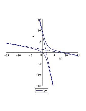
Figure 1: Case 1. $r>\frac{\beta b}{m+\mu}$, for the parameters value $r=0.06,e=0.001,\lambda=0.03,b=250,K=10,\beta=0.0002,m=0.04,\mu=8,\delta=0.02,n=0.007,p=0.08$.

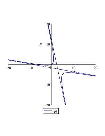
Figure 2: Case 2. $r<\frac{\beta b}{m+\mu}$, for the parameters value $r=0.06,e=0.001,\lambda=0.03,b=1000,K=10,\beta=0.001,m=0.04,\mu=10,\delta=0.02,n=0.007,p=0.08$.

Remark 1.

Observe that the change in the two different shapes of the hyperbola $\psi_{1}$ occurs when the parameter value $r$ crosses the threshold value

$$r_{deg}=\frac{\beta^{2}b^{2}}{\delta K(m+\mu)^{2}}+\frac{\beta b}{m+\mu},$$ (16)

for which the hyperbola degenerates into its asymptotes. However, this has no consequence on the analysis results.

For the second conic section, the first invariant, assumed to be nonvanishing, is

$$\frac{(p-\delta)n\beta b}{4(m+\mu)}+\frac{p\beta^{2}b^{2}}{4(m+\mu)^{2}}\neq 0,$$

while the second one is always negative,

$$-\frac{(-p+\delta)^{2}}{4}<0,$$

showing that also $\psi_{2}$ is a hyperbola. Its center $C^{\prime}$ is

$$x_{c^{\prime}}=\frac{1}{(p-\delta)^{2}}\left[n(\delta-p)-\frac{2p\beta b}{m+\mu}\right],\quad y_{c^{\prime}}=\frac{\beta b}{(p-\delta)(m+\mu)}.$$

Here, the slopes of the asymptotes solve the quadratic equation

$$(\delta-p)l-pl^{2}=0,$$

which provide immediately

$$l_{1}=0,\quad l_{2}=\frac{\delta-p}{p},$$

so that $\psi_{2}$ has the horizontal asymptote

$$N=\frac{\beta b}{(p-\delta)(m+\mu)}.$$

Further, the hyperbola $\psi_{2}$ passes through the origin and crosses the negative vertical axis. There are two possible cases, $p>\delta$ and $p<\delta$. In the former, Case A, the feasible branch raises up monotonically from the origin to the horizontal asymptote, in the latter, Case B, instead it raises up again from the origin to the oblique asymptote.

Hyperbola $\psi_{2}$

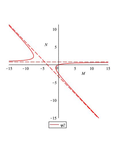
Figure 3: Case A. $p>\delta$, for the parameters value $r=0.06,e=0.001,\lambda=0.03,b=250,K=10,\beta=0.002,m=0.04,\mu=8,\delta=0.002,n=0.2,p=0.08.$.

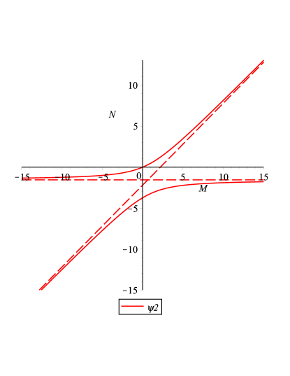
Figure 4: Case B. $p<\delta$, for the parameters value $r=0.06,e=0.001,\lambda=0.03,b=250,K=10,\beta=0.002,m=0.04,\mu=8,\delta=0.08,n=0.15,p=0.04$.

Remark 2.

The change occurs when the hyperbola degenerates into its asymptotes, as the parameter value $\delta$ crosses the critical threshold value

$$\delta_{deg}=p+\frac{\beta bp}{n(m+\mu)}.$$ (17)

But, just as for $\psi_{1}$, this change in shape does not affect the analysis results.

Evidently, the hyperbolae $\psi_{1}$ and $\psi_{2}$ meet at the origin and they further intersect at another point at least, which we require it to be located in the first quadrant for feasibility. The following cases may arise.

• If $r>\frac{\beta b}{m+\mu}$ and $p>\delta$, there is a feasible intersection point.

• If $r>\frac{\beta b}{m+\mu}$ and $p<\delta$, there is a feasible intersection point.

• If $r<\frac{\beta b}{m+\mu}$ and $p>\delta$, two possible situations may occur, the hyperbolae intersect at a feasible point if and only if the slope at the origin of $\psi_{2}$ is larger than that of $\psi_{1}$.

  In this case, the hyperbolae intersect at a feasible point if the slope at the origin of $\psi_{2}$ is larger than that of $\psi_{1}$.The slopes of the two hyperbolae at the origin to be

  $$N^{\prime}_{\psi_{1}}(0)=-1+\frac{\beta b}{r(m+\mu)},\quad N^{\prime}_{\psi_{2}}(0)=\frac{\beta b}{n(m+\mu)}.$$ (18)

  Hence, the condition that they must satisfy is $N^{\prime}_{\psi_{2}}(0)>N^{\prime}_{\psi_{1}}(0)$, which becomes

  $$\beta b(r-n)+rn(m+\mu)>0.$$ (19)

• If $r<\frac{\beta b}{m+\mu}$ and $p<\delta$, two possible situations may occur, again depending on the slopes at the origin of the two conic sections, which give once again condition (19).

In summary, we can conclude that the equilibrium point $E_{5}$ is feasible if (15) holds, or otherwise, but then (19) is satisfied.

The coexistence equilibrium will finally be analysed numerically.

5 Stability

The Jacobian matrix for the system (3) at a generic point is given by

$$J=\left(\begin{array}[]{cccc}J_{11}&-\frac{bB}{(B+I)^{2}}-\gamma B&0&-\lambda B\\ -\frac{bI}{(B+I)^{2}}+\lambda N+\gamma I&J_{22}&0&\lambda B\\ -eM&-\beta M&J_{33}&J_{34}\\ -eN&\beta M&J_{43}&J_{44}\\ \end{array}\right),$$ (20)

where

$$J_{11}=\frac{b}{B+I}-\frac{bB}{(B+I)^{2}}-\lambda N-m-\gamma I$$

$$J_{22}=\frac{b}{B+I}-\frac{bI}{(B+I)^{2}}-m-\mu+\gamma B$$

$$J_{33}=-\frac{r(M+N)}{K}+r(1-\frac{M+N}{K})-\beta I-eB-\delta N$$

$$J_{34}=-\frac{r(M+N)}{K}+r(1-\frac{M+N}{K})-\delta M$$

$$J_{43}=\delta N-pN+\beta I$$

$$J_{44}=-n-eB+\delta M-p(M+N)-pN.$$

We now turn to the stability analysis of each equilibrium. However, in view of the difficulty of analytically assessing even its existence, as already stated above, the stability coexistence equilibrium $E^{*}$ is investigated by means of simulations.

5.1 Stability of $E_{1}$

For the equilibrium point $E_{1}$ the eigenvalues are

$$\Lambda_{1}=-m,\quad\Lambda_{2}=\frac{b\gamma-m\mu}{m},\quad\Lambda_{3}=\frac{mr-be}{m},\quad\Lambda_{4}=-\frac{be+mn}{m}.$$

Therefore, the equilibrium $E_{1}$ is stable if and only if

$$\gamma<\frac{m}{b\mu},\quad r<\frac{be}{m}.$$ (21)

5.2 Stability of $E_{2}$

Two of the eigenvalues of $J$ evaluated at $E_{2}$ are immediately found,

$$\Lambda_{1}=\mu-\frac{\gamma b}{m+\mu}=\frac{m\mu+\mu^{2}-\gamma b}{m+\mu},\quad\Lambda_{2}=-m-\mu.$$

The other two eigenvalues are the roots of the equation

$$\Lambda^{2}-\textrm{tr}\widehat{J}^{*}(E_{2})\Lambda+\det\widehat{J}^{*}(E_{2})=0,$$

where $\textrm{tr}\widehat{J}^{*}(E_{2})$ and $\det\widehat{J}^{*}(E_{2})$ are respectively the trace and the determinant of the submatrix

$$\widehat{J}^{*}(E_{2})=\left(\begin{array}[]{cc}r-\dfrac{b\beta}{m+\mu}&r\\ \dfrac{\beta b}{m+\mu}&-n\\ \end{array}\right),$$

obtained from (20) deleting the first two rows and the first two columns. The Routh-Hurwitz criterion ensures that the eigenvalues have negative real part if and only if

$$\textrm{tr}\widehat{J}^{*}(E_{2})=r-\frac{b\beta}{m+\mu}-n<0,\quad\det\widehat{J}^{*}(E_{2})=\frac{\beta bn}{m+\mu}-rn-\frac{r\beta b}{m+\mu}>0,$$ (22)

which can be rewritten as

$$(r-n)(m+\mu)<b\beta,\quad b\beta(n-r)>rn(m+\mu).$$ (23)

Clearly, we need $n>r$ for the second condition and this implies that the first one holds. Furthermore, for stability also the first eigenvalue $\Lambda_{1}$ must be negative, so the following condition is also necessary, in addition to (23). Therefore, at $E_{2}$ stability occurs if and only if

$$b\gamma-m\mu-\mu^{2}>0,\quad b\beta>(m+\mu)\frac{rn}{n-r},\quad n>r.$$ (24)

5.3 Stability analysis for $E_{3}$

Also for the equilibrium point $E_{3}$ two eigenvalues are explicit, $\Lambda_{1}=-m$, $\Lambda_{2}=-r+\frac{be}{m}<0$ by the feasibility condition (9). The other two eigenvalues are those of the remaining minor of the Jacobian $\widetilde{J}^{*}(E_{3})$. They are the roots of the quadratic

$$\Lambda^{2}-{\textrm{tr}}\widetilde{J}^{*}(E_{3})\Lambda+\det\widetilde{J}^{*}(E_{3})=0.$$

Again, by the Routh-Hurwitz criterion, at $E_{3}$ stability is achieved for

$$\frac{\gamma b}{m}+\left(\frac{\delta K}{r}-\frac{pK}{r}\right)\left(r-\frac{be}{m}\right)<\mu+n+\frac{be}{m}\qquad\qquad$$ (25)

$$\left(\frac{\gamma b}{m}-\mu\right)\left[\left(\frac{\delta K}{r}-\frac{pK}{r}\right)\left(r-\frac{be}{m}\right)-n-\frac{be}{m}\right]>\frac{\lambda b}{m}\frac{bK}{r}\left(r-\frac{be}{m}\right).$$

5.4 Stability analysis for $E_{4}$

The characteristic equation at $E_{4}$ factorizes into the product of two quadratic equations. The first is

$$\Lambda^{2}-{\textrm{tr}}J^{*}(E_{4})\Lambda+\det J^{*}(E_{4})=0,$$ (26)

where $J^{*}(E_{4})$ is the submatrix

$$J^{*}(E_{4})=\left(\begin{array}[]{cc}\dfrac{b\gamma(b\gamma-m\mu-\mu^{2})}{\mu^{3}}&\dfrac{(b\gamma-m\mu-\mu^{2})(b\gamma+\mu^{2})}{\mu^{3}}\\ -\dfrac{(b\gamma-m\mu)(b\gamma-\mu^{2})}{\mu^{3}}&-\dfrac{b\gamma(b\gamma-m\mu)}{\mu^{3}}\\ \end{array}\right).$$

Thus, the Routh Hurwitz conditions give the first set of inequalities needed for stability, the first one of which holds unconditionally:

$${\textrm{tr}}J^{*}(E_{4})= \frac{b\gamma(b\gamma-m\mu-\mu^{2})}{\mu^{3}}-\frac{b\gamma(b\gamma-m\mu)}{\mu^{3}}=-\frac{b\gamma}{\mu}<0,$$ (27)

$$\begin{split}\det J^{*}(E_{4})=&\left(\frac{b\gamma(b\gamma-m\mu-\mu^{2})}{\mu^{3}}\right)\left(-\frac{b\gamma(b\gamma-m\mu)}{\mu^{3}}\right)\\ &+\frac{(b\gamma-m\mu-\mu^{2})(b\gamma+\mu^{2})(b\gamma-m\mu)(b\gamma-\mu^{2})}{\mu^{6}}>0.\end{split}$$ (28)

Dividing (28) by $(b\gamma-m\mu-\mu^{2})(b\gamma-m\mu)$, which is negative from the feasibility condition (9), the inequality is reduced to

$$-\frac{1}{\mu^{2}}<0,$$

so that it always holds. The second quadratic is

$$\Lambda^{2}-{\textrm{tr}}J_{*}(E_{4})\Lambda+\det J_{*}(E_{4})=0,$$ (29)

where

$$J_{*}(E_{4})=\left(\begin{array}[]{cc}r-\dfrac{\beta(b\gamma-m\mu)+e(-b\gamma+m\mu+\mu^{2})}{\mu\gamma}&r\\ \dfrac{\beta(b\gamma-m\mu)}{\mu\gamma}&\dfrac{e(b\gamma-m\mu-\mu^{2})}{\mu\gamma}-n\\ \end{array}\right).$$ (32)

Once again, the associated Routh-Hurwitz conditions

$$\begin{split}{\textrm{tr}}J_{*}(E_{4})&=r-\frac{\beta(b\gamma-m\mu)}{\mu\gamma}+\frac{2e(b\gamma-m\mu-\mu^{2})}{\mu\gamma}-n<0,\end{split}$$

$$\begin{split}\det J_{*}(E_{4})=&\left(r-\frac{\beta(b\gamma-m\mu)+e(-b\gamma+m\mu+\mu^{2})}{\mu\gamma}\right)\left(\frac{e(b\gamma-m\mu-\mu^{2})}{\mu\gamma}-n\right)\\ &-\frac{r\beta(b\gamma-m\mu)}{\mu\gamma}>0,\end{split}$$

upon rearranging, provide the following stability conditions:

$$r+\frac{2e(b\gamma-m\mu-\mu^{2})}{\mu\gamma}<n+\frac{\beta(b\gamma-m\mu)}{\mu\gamma},$$ (33)

$$\left(r-\frac{\beta(b\gamma-m\mu)+e(-b\gamma+m\mu+\mu^{2})}{\mu\gamma}\right)\left(\frac{e(b\gamma-m\mu-\mu^{2})}{\mu\gamma}-n\right)$$

$$>\frac{r\beta(b\gamma-m\mu)}{\mu\gamma}.$$

5.5 Stability analysis for $E_{5}$

For the equilibrium point $E_{5}$ the analytic expression of the mite populations $M_{5}$ and $N_{5}$ is not know. Anyway, we can evaluate the Jacobian matrix (20) for $B=0$ and $I=\frac{b}{m+\mu}$. The characteristic equations factorizes to provide immediately two eigenvalues, namely

$$\Lambda_{1}=\mu-\lambda N-\frac{\gamma b}{m+\mu},\quad\Lambda_{2}=-m-\mu,$$

yielding the first stability condition

$$N>\frac{1}{\lambda}\left(\mu-\frac{\gamma b}{m+\mu}\right).$$ (34)

The other two eigenvalues are the roots of

$$\Lambda^{2}-{\textrm{tr}}\overline{J}^{*}(E_{5})\Lambda+\det\overline{J}^{*}(E_{5})=0$$

where $\overline{J}^{*}(E_{5})$ is the submatrix

$$\overline{J}^{*}(E_{5})=\left(\begin{array}[]{cc}\overline{J}_{33}&r-\frac{2r}{K}(M+N)-\delta M\\ \delta N-pN+\frac{\beta b}{m+\mu}&\overline{J}_{44}\\ \end{array}\right),$$

obtained from (20) deleting the first two rows and columns and

$$\overline{J}_{33}=r-\frac{2r}{K}(M+N)-\frac{\beta b}{m+\mu}-\delta N,\quad\overline{J}_{44}=-n+(\delta-p)M-2pN.$$

The Routh-Hurwitz criterion provide the remaining stability conditions

$$M\left(-\frac{2r}{K}+\delta-p\right)+N\left(-\frac{2r}{K}-\delta-2p\right)+r<n+\frac{\beta b}{m+\mu},$$ (35)

$$\left[r-\frac{2r}{K}(M+N)-\frac{\beta b}{m+\mu}-\delta N\right]\left[-n+(\delta-p)M-2pN\right]$$

$$>\left[r-\frac{2r}{K}(M+N)-\delta N\right]\left[(\delta-p)N+\frac{\beta b}{m+\mu}\right].$$

6 Numerical simulations and interpretation

In this section, after describing the set of parameter values used, we carry out numerical simulations using the built-in ordinary differential equations solver ode45.

6.1 The model parameters

We take some model parameters from the literature, [7], [10], [1] and [6].

Taking the day as the time unit, the birth rate of worker honey bees is taken as $b=2500$, while their natural mortality rate is $m=0.04$, equivalent to a life expectancy of $25$ days, [7].

The literature does not provide a precise value for the grooming behavior, but from [7] a range of reasonable values of $e$ lies between $10^{-6}$ and $10^{-5}$.

During the bee season, i.e. spring and summer, the mite population doubles every month, so we fix $r\approx\ln 2\div 30$, that is $r=0.02$, [6].

Their carrying capacity is taken as $K=15000$ mites, [10], while their natural mortality rate in the phoretic phase is estimated to be $n=0.007$ during the bee season, [1].

Table (1) summarizes these values, that are used in the numerical simulations.

Parameter	Interpretation	Value	Unit	Source
$b$	Bee daily birth rate	$2500$	$bees\times day^{-1}$	[7]
$e$	Grooming rate of healthy bee	$10^{-6}-10^{-5}$	$day^{-1}$	[7]
$m$	Bee natural mortality rate	$0.04$	$day^{-1}$	[7]
$K$	Varroa carrying capacity	$15000$	$mites$	[10]
$r$	Varroa growth rate	$0.02$	$day^{-1}$	[6]
$n$	Varroa natural mortality	$0.007$	$day^{-1}$	[1]
	rate in the phoretic phase

Table 1: Model parameters

6.2 Discussion

The initial conditions for the colony are given from field data. All the bees are healthy since the infected, having a lower longevity, cannot survive the winter. Further, the acaricide treatments against Varroa performed in the autumn and winter theoretically allow to eradicate the infestation, so that the mite population usually does not exceed $10$ units at the beginning of the bee season.

Population	Value
Sound bees	$15000$
Infected bees	$0$
Mites	$\leq 10$

Table 2: Initial condition for simulations

For the parameters $b,e,m,K,r,n$ we use the reference values from the real situation described in the previous section, see Table (1). The remaining parameter values are arbitrarily chosen to simulate a hypothetical hive.

6.3 Equilibrium $E_{1}$

At the equilibrium $E_{1}$ only the healthy bees survive. It represents the best situation for the hive. Healthy and infected mites are wiped out while the healthy bee population increases to a level of $62500$ units.

The equilibrium $E_{1}$ is stably attained for the following choice of parameters: $r=0.02$, $K=15000$, $b=2500$, $m=0.04$, $n=0.007$, $e=0.00001$, $\mu=8$, $\lambda=0.3$; $\delta=0.0001$, $\beta=0.1$, $\gamma=0.0001$, $p=0.04$. Initial conditions $B=15000$, $I=0$, $M=3$, $N=2$.

The second stability condition (21) is always satisfied by the field data. Infected bees become extinct in view of the remaining stability condition (21), that, rewritten in the form $\gamma<m\mu b^{-1}$, establishes an upper bound on the horizontal transmission rate of the virus among bees.

6.4 Equilibrium $E_{2}$

It is interesting to note that the equilibrium point $E_{2}$, in which the disease affects the whole bee colony but the mites disappear, is unstable when the field data are used, since the third stability condition (24) is not satisfied. Indeed note that $n-r=0.007-0.02<0$.

6.5 Equilibrium $E_{3}$

Also the disease-free equilibrium point $E_{3}$, in which healthy mites are present, is infeasible in the field conditions, since the feasibility condition (9) is not satisfied.

This result is well substantiated by the empirical beekeepers observations in natural honey bee colonies. Namely, the viral infection occurs whenever the mite population is present.

6.6 Equilibrium $E_{4}$

At the mite-free equilibrium point $E_{4}$ the disease remains endemic among the bees.

Rearranging (33), we can see that in this situation the opposite condition of equilibrium $E_{1}$ must be verified, namely

$$\frac{m\mu}{b}<\gamma<\frac{\mu^{2}+m\mu}{b}$$ (36)

imposing a lower and an upper bound on the disease horizontal transmission rate among bees. It is indeed reasonable to expect that also the population of infected bees survives, as opposed to the equilibrium $E_{1}$, with a high enough contact rate.

If the horizontal transmission rate becomes too large though, exceeding its upper bound, the point $E_{4}$ becomes unstable, but the first stability condition for $E_{2}$, (21), holds. Apparently we could obtain the equilibrium $E_{2}$ in which the infection affects all the honey bees, but we already know that $E_{2}$ is always unstable from the field data and therefore the infected bees in such situation do not thrive alone in the hive.

The equilibrium $E_{4}$ is obtained for the parameters values: $r=0.02$, $K=15000$, $b=2500$, $m=0.04$, $n=0.007$, $e=0.00001$,$\mu=6$, $\lambda=0.01$; $\delta=0.0005$, $\beta=0.00006$, $\gamma=0.0002$, $p=0.001$ and the initial conditions $B=15000$, $I=0$, $M=3$, $N=2$. The eigenvalues of the Jacobian matrix for these parameter values are

$$\Lambda_{1}\approx-0.0416+0.5i\quad\Lambda_{2}\approx-0.0416-0.5i\quad\Lambda_{3}\approx-0.28\quad\Lambda_{4}\approx-0.31.$$

showing that there are damped oscillations.

6.7 Equilibrium $E_{5}$

The equilibrium $E_{5}$ represents the Varroa invasion scenario. It is always feasible by the field data, since (19) is always satisfied, as its left hand side is $r-n=0.02-0.007>0$. It can be obtained with the following choice for the parameters: $r=0.02$, $K=15000$, $b=2500$, $m=0.04$, $n=0.007$, $e=0.00001$,$\mu=5$, $\lambda=0.004$; $\delta=0.0005$, $\beta=0.0001$, $\gamma=0.3$, $p=0.0003$ and the initial conditions $B=15000$, $I=0$, $M=3$, $N=2$.

Also in this case, the viral infection remains endemic. The effective virulence of the disease is increased by the presence of mites, since the virus is directly vectored into the hemolymph of the honey bees. As a consequence, the healthy bee population becomes extinct.

Since $E_{2}$ is unstable in view of the field data, it seems much more likely that an epidemic could affect all the bees in a Varroa-infested colony than in a Varroa-free colony.

In fact, the mite is a far more effective vector than nurse bees are. Further, detailed studies show that most of honey bee viruses are present at low levels but do not cause any apparent symptoms in Varroa-free colonies. Only important stressors, such as the introduction of Varroa destructor, can convert the silent infection into a symptomatic one, [9].

6.8 The coexistence equilibrium $E^{*}$

At coexistence the honey bees share their infected hive with mites.

Figures (5) and (6) show two different levels of infection. The spread of the virus throughout the colony depends on model parameters describing the disease transmission, namely $\lambda$, $\gamma$, $\beta$, $\delta$. Reasonably, small values of these parameters lead to a rather higher prevalence of healthy bees and mites with respect to the infected ones, Figure (5), while the opposite situation is depicted in Figure (6) in presence of higher disease transmission rates. Furthermore, comparing the $\mu$-values in these simulations, we discover an interesting and seemingly counter-intuitive phenomenon: a higher level of infection in the hive is obtained for a lower value of the disease-related mortality and vice versa. This can be interpreted by observing that a higher survival of infected bees makes them longer available for the transmission of the virus and inevitably leads to an increase of the viral titer in the colony. Hence, when transmitted by Varroa mites, the most virulent diseases at the colony level become the least harmful for the single bees. Thus the number of mites required for vectoring an epidemic spread is higher for the most harmful viruses. It has indeed been shown, for example, that the acute paralysis virus (APBV), which is rapidly lethal to infected bees, requires a much larger mite population for its outbreak of an epidemic than the mite population needed for the deformed wing virus (DWV) outbreak, which allows a greater survival of infected bees [13].

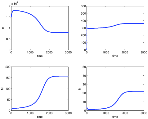
Figure 5: The coexistence equilibrium $E^{*}$, for the parameters values: $r=0.02$, $K=15000$, $b=2500$, $m=0.04$, $n=0.007$, $e=0.000001$,$\mu=6$, $\lambda=0.007$; $\delta=0.0005$, $\beta=0.00001$, $\gamma=0.0003$, $p=0.0005$. Initial conditions $B=15000$, $I=0$, $M=6$, $N=4$.

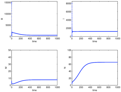
Figure 6: The coexistence equilibrium $E^{*}$, for the parameters values: $r=0.02$, $K=15000$, $b=2500$, $m=0.04$, $n=0.007$, $e=0.000001$,$\mu=2$, $\lambda=0.01$; $\delta=0.001$, $\beta=0.0001$, $\gamma=0.0006$, $p=0.0002$. Initial conditions $B=15000$, $I=0$, $M=6$, $N=4$.

Finally, in Figure (7) we use a different initial condition from the previous simulations to highlight the effect of Varroa infestation on honey bee viral infections: here the bee population drastically decreases as the mites increase. For a high value for the disease-related mortality of the bees ($\mu=7$), we observe a low level of infection, with the infected bees not exceeding $350$, although the decrease of healthy bees is quite dramatic.

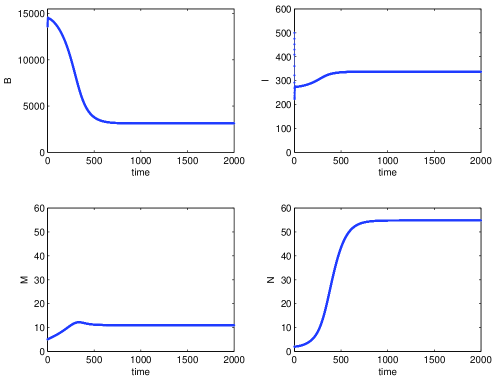
Figure 7: The coexistence equilibrium $E^{*}$, for the parameters values: $r=0.02$, $K=15000$, $b=2500$, $m=0.04$, $n=0.007$, $e=0.000001$,$\mu=7$, $\lambda=0.01$; $\delta=0.002$, $\beta=0.00002$, $\gamma=0.0004$, $p=0.0002$. Initial conditions $B=14000$, $I=500$, $M=5$, $N=2$.

6.9 Summary

We sum up the feasibility and stability conditions of the equilibrium points in Table 3.

Equilibrium	Feasibility	Stability	In field
			conditions
$E_{1}$	always	(21)	allowed
$E_{2}$	always	(24)	unstable
$E_{3}$	(9)	(25)	infeasible
$E_{4}$	(11)	(33)	allowed
$E_{5}$	(15) or, otherwise, (19)	(34), (35)	allowed
$E^{*}$	numerical	numerical	allowed
	simulations	simulations

Table 3: Summarizing table of equilibria: feasibility and stability conditions

7 Bifurcations

7.1 Transcritical bifurcations

Direct analytical considerations on the feasibility and stability conditions are only possible between $E_{1}$ and $E_{4}$. Some other transcritical bifurcations are found with the help of numerical simulations.

• $E_{1}$-$E_{4}$

  Comparing (21) and the left inequality in (11), we find that $E_{4}$ becomes feasible exactly when $E_{1}$ is unstable, and vice versa. There is thus a transcritical bifurcation for which $E_{4}$ emanates from $E_{1}$ when the bifurcation parameter $\gamma$ crosses from below the critical value $\gamma^{\dagger}$ given by

  $$\gamma^{\dagger}=\frac{m\mu}{b}.$$ (37)

  The simulation reported in Figure (8) shows it explicitly. For the chosen parameter values, $\gamma^{\dagger}=\frac{m\mu}{b}\approx 0.000097$.

  

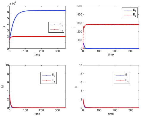
  Figure 8: Transcritical bifurcation between $E_{1}$ and $E_{4}$, for the parameters values $r=0.02$, $K=15000$, $b=2500$, $m=0.04$, $n=0.007$, $e=0.00001$,$\mu=6$, $\lambda=0.01$, $\delta=0.0005$, $\beta=0.00006$, $\gamma=0.000094$ (blue), $\gamma=0.0003$ (red), $p=0.001$. Initial conditions $B=15000$, $I=0$, $M=3$, $N=2$.

• $E_{2}$-$E_{4}$

  Another transcritical bifurcation arises between $E_{2}$ and $E_{4}$, compare the first (24) and the right inequality in (11). It occurs for the critical bifurcation parameter value

  $$\gamma^{\ddagger}=\mu\frac{m+\mu}{b}.$$ (38)

• $E_{2}$-$E_{5}$

  Further, comparing the second (24) and (19), also between $E_{2}$ and $E_{5}$ we find anew a transcritical bifurcation. In this case $E_{5}$ emanates from $E_{2}$ when the disease transmission rate between infected bees and susceptible mites falls below the critical value

  $$\beta^{\dagger}=\frac{m+\mu}{b}\frac{rn}{n-r}.$$ (39)

• $E_{4}$-$E^{*}$

  Numerically, a transition is seen to occur between the equilibrium $E_{4}$ and the coexistence point $E^{*}$. It is shown in Figure (9), taking as bifurcation parameter $\mu$.

  As we have observed in the previous section, a low value of the disease-related mortality allows infected bees to survive longer. Instead, a higher value of $\mu$ causes a drastic reduction of the infected bee population. As a consequence, although there is a harmful epidemic, the bee population is not greatly affected at the colony level and mites are soon groomed away by the healthy bees.

  

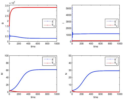
  Figure 9: Transcritical bifurcation between $E_{4}$ and $E^{*}$, for the parameters values $r=0.02$, $K=15000$, $b=2500$, $m=0.04$, $n=0.007$, $e=0.000001$,$\mu=2$ (blue), $\mu=10$ (red) $\lambda=0.007$, $\delta=0.0005$, $\beta=0.00001$, $\gamma=0.0003$, $p=0.0005$. Initial conditions $B=15000$, $I=0$, $M=3$, $N=2$.

• $E_{1}$-$E_{5}$

  In Figure (10), another transcritical bifurcation is shown. For a small value of $\gamma$ the system settles to the disease- and mite-free equilibrium $E_{1}$. For a significantly higher value of $\gamma$, mites invade the environment, the disease becomes endemic and no healthy bees survive, equilibrium $E_{5}$.

  

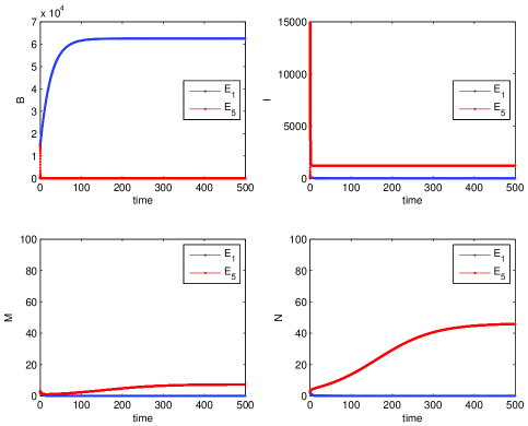
  Figure 10: Transcritical bifurcation between $E_{1}$ and $E_{5}$, for the parameters values $r=0.02$, $K=15000$, $b=2500$, $m=0.04$, $n=0.007$, $e=0.00001$,$\mu=2$, $\lambda=0.004$, $\delta=0.0005$, $\beta=0.0001$, $\gamma=0.00002$ (blue), $\gamma=0.3$ (red), $p=0.0003$. Initial conditions $B=15000$, $I=0$, $M=3$, $N=2$.

• $E_{5}$-$E^{*}$

  In Figure (11) we discover that a transition can occur also between $E_{5}$ and $E^{*}$, if the horizontal transmission rate of the virus among honey bees $\gamma$ is low enough. In such case indeed the healthy bees can thrive in the hive.

  

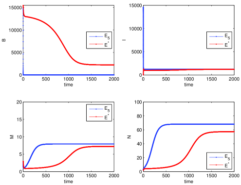
  Figure 11: Transcritical bifurcation between $E_{5}$ and $E^{*}$, for the parameters values $r=0.02$, $K=15000$, $b=2500$, $m=0.04$, $n=0.007$, $e=0.000001$, $\mu=2$, $\lambda=0.01$, $\delta=0.001$, $\beta=0.0001$, $\gamma=0.03$ (blue), $\gamma=0.0001$ (red), $p=0.0002$. Initial conditions $B=15000$, $I=0$, $M=3$, $N=2$.

• $E_{1}$-$E^{*}$

  Finally, in Figure (12), we can see that the system can change its behavior going directly from $E_{1}$ to $E^{*}$, again by suitably tuning the parameter $\gamma$.

  

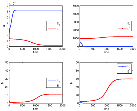
  Figure 12: Transcritical bifurcation between $E_{1}$ and $E^{*}$, for the parameters values $r=0.02$, $K=15000$, $b=2500$, $m=0.04$, $n=0.007$, $e=0.000001$, $\mu=2$, $\lambda=0.01$, $\delta=0.0001$, $\beta=0.0001$, $\gamma=0.00002$ (blue), $\gamma=0.0001$ (red), $p=0.0002$. Initial conditions $B=15000$, $I=0$, $M=3$, $N=2$.

We also provide a bifurcation diagram for the four populations as a function of the bifurcation parameter $\gamma$ in Figure (13). Starting from very low values of $\gamma$, we find at first the healthy-bees-only equilibrium $E_{1}$. Note that only the healthy bee population $B$ thrives when $\gamma<\gamma^{\dagger}\approx 5\cdot 10^{-5}$. Then in the range $\gamma^{\dagger}<\gamma<\gamma_{1}\approx 1.4\cdot 10^{-4}$ the disease becomes endemic, thus $I>0$, while mites keep on being wiped out. The system is found thus at equilibrium $E_{4}$. For values of $\gamma$ larger than $\gamma_{1}$ and up to $\gamma_{2}\approx 3\cdot 10^{-3}$, the system quickly settles at the equilibrium $E^{*}$. Here we have coexistence of bees and mites in an endemic hive, all the populations survive. Past the threshold value $\gamma_{2}$ the healthy bee population vanishes. In this situation, the disease remains endemic and affects all the bees. This last transition shows numerically that we have another transcritical bifurcation between the coexistence and the Varroa invasion situations, namely the equilibria $E^{*}$ and $E_{5}$.

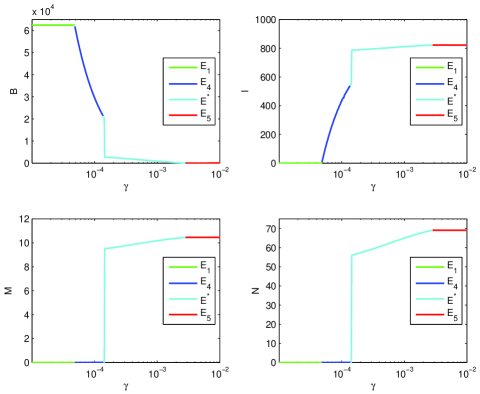
Figure 13: Bifurcation diagram, for the parameters values $r=0.02$, $K=15000$, $b=2500$, $m=0.04$, $n=0.007$, $e=0.000001$, $\mu=3$, $\lambda=0.01$, $\delta=0.001$, $\beta=0.0001$, $p=0.0002$. Initial conditions $B=15000$, $I=0$, $M=3$, $N=2$.

7.2 Hopf bifurcations

We now try to establish whether there are special parameter combinations for which sustained population oscillations are possible. For this purpose, the eigenvalues must cross the imaginary axis.

This is easy to assess for a quadratic characteristic equation, $\Lambda^{2}+b\Lambda+c=0$, since we need the linear term to vanish, $b=0$, and the constant term to be positive, $c>0$.

Clearly at $E_{1}$ no Hopf bifurcation arises, since the eigenvalues are all real.

At $E_{4}$ the characteristic equation factors into the product of two quadratics. The first one, namely the equation (26), has a negative linear term so we exclude the possibility for a Hopf bifurcation to occur.

The second one has the form (29). To see whether Hopf bifurcation arise, we need the trace to vanish and the determinant to be positive. Thus, imposing the condition on the trace we are led to

$$r-\frac{\beta(b\gamma-m\mu)}{\mu\gamma}+\frac{2e(b\gamma-m\mu-\mu^{2})}{\mu\gamma}-n=0,$$ (40)

This condition however contradicts the second stability condition (33). Indeed, note that solving for $n$ the equation (40), we find

$$n=r-\frac{\beta(b\gamma-m\mu)}{\mu\gamma}+\frac{2e(b\gamma-m\mu-\mu^{2})}{\mu\gamma},$$ (41)

and the second inequality in (33) becomes

$$-\left(r-\frac{\beta(b\gamma-m\mu)+e(-b\gamma+m\mu+\mu^{2})}{\mu\gamma}\right)^{2}-\frac{r\beta(b\gamma-m\mu)}{\mu\gamma}>0,$$

which is never satisfied, using the left inequality in the feasibility condition (11). We conclude that at $E_{4}$ no Hopf bifurcations can arise.

8 Sensitivity analysis

In this section we perform the sensitivity analysis on (3) in order to rank the parameters with respect to their influence on the system dynamics.

The first step is to determine the sensitivity equations by differentiating the original equations with respect to all the parameters. Our model consists of 4 equations with 12 parameters, therefore we get a sensitivity system of 48 equations.

In fact, [2], when defining $\alpha$ the vector of the 12 parameters, the sensitivity system for (2) can be formulated as

$$\frac{d}{dt}\left(\frac{\partial X_{i}(\alpha,t)}{\partial\alpha_{j}}\right)=\sum_{s=1}^{4}\frac{\partial f_{i}(X,\alpha,t)}{\partial X_{s}}\frac{\partial X_{s}(\alpha,t)}{\partial\alpha_{j}}+\frac{\partial f_{i}(X,\alpha,t)}{\partial\alpha_{j}},$$ (42)

for $i=1,\dots,4$ and $j=1,\dots,12$, with initial conditions

$$\frac{\partial X_{i}(\alpha,0)}{\partial\alpha_{j}}=0,\quad i=1,\dots,4,\quad j=1,\dots,12.$$ (43)

Note that solving such system requires the knowledge of the state variables $X_{i},i=1\dots,4$ and therefore it involves also the solution of the system (3). Finally, we are led to solve a system of $52$ differential equations.

The rate of change of the state as a function of the change in the chosen parameter is obtained from the value of the sensitivity solution evaluated at time $t$, [3].

However, the parameters, and thus also the sensitivity solutions for different parameters, are measured in different units. This means that without further action, any comparison is futile. To make a valid comparison of the effect that parameters with different units have on the solution, we simply multiply the sensitivity solution by the parameter under consideration. This form of the sensitivity function is known as the semi-relative sensitivity solution, [4]. It provides information concerning the amount of change that the population will experience when the parameter of interest is subject to a positive perturbation, [3].

Computing the semi-relative solutions and making a comparison of the scales on the vertical axis of these plots (formally, this is equivalent to ranking the parameters according to the $\infty-$norm), we deduce that the parameters most affecting the system are $r,\mu$ and $\gamma$.

Specifically, an increase of the Varroa growth rate has a negative effect on the bee population and a positive influence on the mite population, consistently with Figure (14) (left frame). Furthermore, the effect of perturbing $r$ can be observed best on the population of healthy bees and results in a reduction of $1200$ units (bees) after $210$ days.

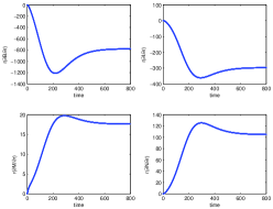
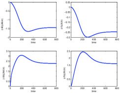
Figure 14: Semi-relative solutions (left) and the logarithmic sensitivity solutions (right) with respect to the parameter $r$.

From Figure (14) (right frame), we can approximatively get the expected percentage changes from an increase of $r$. In particular, [3], we compute the logarithmic sensitivity solutions, namely

$$\frac{\partial\log(X_{i}(\alpha,t))}{\partial\log(\alpha_{j})}=\frac{\alpha_{j}}{X_{i}(\alpha,t)}\frac{\partial X_{i}(\alpha,t)}{\partial\alpha_{j}},$$ (44)

for $i=1,\dots,4$ and $j=1,\dots,12$.

Calculating (44), we find that a positive perturbation of $r$ leads to a decrease of up to 170% in the healthy bee population at $t=310$ days, a 30% decrease in the infected bee population at $t=290$ days, a 300% increase in the healthy mite population at $t=200$ days, and a 250% increase in the infected mite population at $t=200$ days.

However, we also note that over 200% changes, at time $200$ days, in the mite populations are not significant due to their low level of concentration at time $200$ days in the solution. This is shown in Figure (6) for the set of parameter values used to perform sensitivity analysis.

We now turn to the parameter $\mu$, second in order of sensitivity. From Fig. (15), it is clear that a higher value for the disease-related mortality of the bees has a positive impact on the healthy bee population and a negative influence on the infected bee population. In particular, at the end of the observation period we find an increase of $1000$ units (about 200%) in the healthy bee population and a reduction of $600$ units (less than 50%) in the infected bee population.

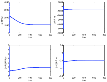
Figure 15: Semi-relative solutions (top) and logarithmic sensitivity solutions (bottom) for the populations B (left) and I (right) with respect to the parameter $\mu$.

According to our results, an increase in $\mu$ inevitably leads to a decrease in the infected bee population. The shorter time of survival means that there is also less time for the virus to be transmitted. This gives an explanation for the positive impact on the healthy bee population. This is in line with our earlier observations: when transmitted by Varroa mites, the most virulent diseases at the colony level are the least harmful ones to the single bees.

Lastly we find the negative influence of $\gamma$ on the population of healthy bees with an expected decrease of $600$ units and a percentage change of about 100% at the end of the observation period, as shown in Fig. (16).

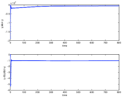
Figure 16: Semi-relative solution (top) and logarithmic sensitivity solution (bottom) for the population B with respect to the parameter $\gamma$.

To conclude the analysis, we look at Fig. (17). Both a positive change in the Varroa natural mortality rate, $n$, as well as in their intraspecific competition coefficient, $p$, have a positive effect on the healthy bee population and, unexpectedly, also on the infected bee population. This suggests that the horizontal transmission of the virus among honey bees would increase the infected bee population also for higher values of $n$ and $p$, i.e. for a lower level of Varroa infestation. The influence of the parameter $\gamma$ on the bee population also explains the frame on the bottom: even a positive perturbation in the honey bee birth rate will yield a decrease in the population of healthy bees, which soon leave this class to benefit the population of the infected ones. Furthermore, the latter is really sensitive with respect to $b$, with a dramatic increase of about $1200$ units (100%) as early as time $t=10$.

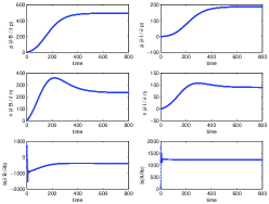
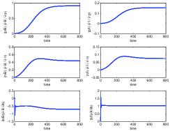
Figure 17: Semi-relative solutions (left) and logarithmic solutions (right) for the populations B and I with respect to the parameters $p$, $n$ and $b$.

Remark 3.

The parameter of interest is usually perturbed by doubling or halving it, in order to understand how sensitive the system dynamics are to such changes in it. Therefore, for each parameter we perform the sensitivity analysis doubling and halving it to find out that the effect of these perturbations is always the same and sensitivity solution plots differ only by the scale on the temporal axis. In particular, doubling parameters yields to a shorter temporal scale, while a longer one is obtained by halving them.

The knowledge of the most influential parameters allows us to understand on which one of them we could act in order to drive the system to a safer situation. From a theoretical point of view, we can conclude that the population of healthy bees would benefit from both a reduction in the Varroa growth rate, as well as a reduction in the horizontal transmission rate among bees.

9 Conclusion

Field and research evidence indicate that the long-term decline of managed honey beehives in the western countries is associated with the presence of viruses in the honey bee populations, [9]. While formerly the viruses produced only covert infections, their combination with the invading parasite Varroa destructor has triggered the emergence of overt viral infections. These cause concern because they entail fatal symptoms at both the individual bee level and at the colony level, constituting a major global threat for apiculture.

In model presented here we combine bee and mite population dynamics with viral epidemiology, to produce results that match field observations well and give a clear explanation of how Varroa affects the epidemiology of certain naturally occurring bee viruses, causing considerable damages to colonies.

In the model, there are only four possible stable equilibria, using the known field parameters, see Table 3. The first one contains only the thriving healthy bees. Here the disease is not present and also the mites are wiped out. Alternatively, there is another equilibrium where the mite population still disappears, but the disease remains endemic among the bee population that survives. Thirdly, infected bees coexist with the mites in the Varroa invasion scenario; in this situation the disease invades the hive, affecting all the bees and driving the healthy bees to extinction. The final coexistence equilibrium is also possible, with both populations of bees and mites thriving and with an endemic disease in the beehive among both species. Transcritical bifurcations relate these points while, in spite of the four dimensionality of the system, which may render them more likely, Hopf bifurcations have been shown not to arise.

Further, two alternatives turn out to be impossible by the use of field data for the parameter values.

On the one hand, the endemic disease cannot affect all the bees in a Varroa-free colony. According to the envisioned role of V. destructor as disease vector for increasing virulence of honey bee viruses, from the analysis the disappearance of whole healthy bee population in a Varroa-infested colony seems much more likely than in a Varroa-free colony.

On the other hand, the healthy mites cannot thrive only with healthy bees. Namely, if the Varroa population is present, then necessarily the bees viral infection occurs.

The findings of this study also indicate that a low horizontal virus transmission rate among honey bees in beehives will help in protecting the bee colonies from the Varroa infestation and the viral epidemics.

The model presented here gives good qualitative insight into the spread of the bee disease. However, in its assumptions certain effects that can be relevant are omitted. Therefore, its primary value lies in the context of qualitative understanding rather than that of a quantitative prediction. For instance, the simulations use constant parameter values, but it remains to be investigated whether the qualitative results would change if continuously changing parameters instead were considered.

Similarly, also the intraspecific competition coefficient among Varroa $p$, taken here as constant, could reasonably be considered as a bee-population-dependent function, since mites essentially compete for the host hemolymph.

Nevertheless, despite this simplicity the model presented here might be a good starting point for the development of other more sophisticated models including seasonality and other aspects relevant for the bee colony health, or for example to investigate the effectiveness of various Varroa treatment strategies.

References

- [1] M. A. Benavente, R. R. Deza, M. Eguaras, Assessment of Strategies for the Control of the Varroa destructor mite in Apis mellifera colonies, through a simple model, MACI, 2 (2009), 5-8.
- [2] V. Comincioli, Metodi numerici e statistici per le scienze applicate (Numerical and statistical methods for applied sciences), Università degli studi di Pavia, 2004.
- [3] D. M. Bortz, P. W. Nelson, Sensitivity analysis of a nonlinear lumped parameter model of HIV infection dynamics, Bulletin of mathematical biology 66(5) (2004), 1009-1026.
- [4] H. T. Banks, D. M. Bortz, A parameter sensitivity methodology in the context of HIV delay equation models, Journal of Mathematical Biology 50(6), (2005), 607-625.
- [5] G. Sabetta, E. Perracchione, E. Venturino, Wild herbivores in forests: four case studies, submitted for publication.
- [6] C. Costa, E. Carpana, M. Lodesani, A. Nanetti, Patologie e Avversità delle Api: tecniche diagnostiche e di campionamento (Pathologies and adversity of bees: diagnostical and sampling techniques), Unità di ricerca di Apicoltura e Bachicoltura (CRA-API).
- [7] J. S. Figueiró, F. C. Coelho, The role of resistance behaviors in the population dynamics of Honey Bees infested by Varroa Destructor, Abstract Collection, Models in Population Dynamics end Ecology, International Conference, Università di Torino, Italy, August 25th-29th 2014, 23.
- [8] J. S. Figueiró, F. C. Coelho, P. A. Bliman, Behavioral modulation of the coexistence between Apis mellifera and Varroa destructor: A defense against colony collapse disorder?, submitted for publication, private communication, 2015.
- [9] E. Genersch, M. Aubert, Emerging and re-emerging viruses of the honey bee (Apis mellifera L.), 2010, Veterinary Research 41, 54.
- [10] S. J. Martin, The role of Varroa and viral pathogens in the collapse of honeybee colonies: a modelling approach, Journal of Applied Ecology 2001, 38, 1082-1093.
- [11] P. A. Moore, M. E. Wilson, J. A. Skinner, Honey Bee Viruses, the Deadly Varroa Mite Associates, 2014, Department of Entomology and Plant Pathology, the University of Tennessee, Knoxville TN. http://www.extension.org/pages/71172/honeybee-viruses-the-deadly-varroa-mite-associates#.VJ2K7l4DI
- [12] V. Ratti, P. G. Kevan, H. J. Eberl, A mathematical model for population dynamics in honeybee colonies infested with Varroa destructor and the Acute Bee Paralysis Virus, 2012, to appear in Canadian Applied Mathematics Quarterly.
- [13] D. J. T. Sumpter, S.J. Martin, The dynamics of virus epidemics in Varroa-infested honey bee colonies, 2004, Journal of Animal Ecology 73, 51-63.
- [14] U. Vesco, Centro di Riferimento Tecnico per l’Apicoltura Patologie Apistiche: Varroa e Patogeni, accoppiata mortale, (Technical Reference Center for apiculture Bees Pathologies: Varroa and Pathogens, a deadly coupling), L’Apis 2, 2013, 5-10.