Superballistic center-of-mass motion in one-dimensional attractive Bose gases: Decoherence-induced Gaussian random walks in velocity space

Abstract

We show that the spreading of the center-of-mass density of ultracold attractively interacting bosons can become superballistic in the presence of decoherence, via single-, two- and/or three-body losses. In the limit of weak decoherence, we analytically solve the numerical model introduced in [Phys. Rev. A 91, 063616 (2015)]. The analytical predictions allow us to identify experimentally accessible parameter regimes for which we predict superballistic spreading of the center-of-mass density. Ultracold attractive Bose gases form weakly bound molecules; quantum matter-wave bright solitons. Our computer-simulations combine ideas from classical field methods (“truncated Wigner”) and piecewise deterministic stochastic processes. While the truncated Wigner approach to use an average over classical paths as a substitute for a quantum superposition is often an uncontrolled approximation, here it predicts the exact root-mean-square width when modeling an expanding Gaussian wave packet. In the superballistic regime, the leading-order of the spreading of the center-of-mass density can thus be modeled as a quantum superposition of classical Gaussian random walks in velocity space.

I Introduction

Superballistic motion (motion with increasing velocities) has been investigated in the context of random walks with random velocities Zaburdaev et al. (2008), driven magnetic turbulence Zimbardo et al. (2000), atom-photon interactions in cavity QED Prants et al. (2002) and nonergodic noise Liu and Bao (2014). In quantum systems, time-dependent random potentials have been demonstrated to cause superballistic transport Levi et al. (2012). Superballistic transport was predicted theoretically in the dynamics of wave-packet spreading in a tight-binding lattice junction Hufnagel et al. (2001); Zhang et al. (2012) and observed experimentally in a hybrid photonic lattice setup Stützer et al. (2013). For a relativistic kicked-rotor system, superballistic transport occurs both in the classical and quantum regime Zhao et al. (2014).

The present paper provides an analytical solution of the numerical model for the spreading of the center-of-mass density of a quantum bright soliton under the influence of decoherence via particle losses introduced in Ref. Weiss et al. (2015a). The analytic approach presented here is valid in the limit that few particles (compared to the total number of particles) are lost. We use this approach to identify experimentally realistic parameters for which we predict that superballistic spreading of the center-of-mass density can be observed experimentally.

Bright solitons can be experimentally generated from attractively interacting ultracold atomic gases Khaykovich et al. (2002); Strecker et al. (2002); Cornish et al. (2006); Marchant et al. (2013); Medley et al. (2014); McDonald et al. (2014); Nguyen et al. (2014); Marchant et al. (2016); Everitt et al. (2015); on the mean-field level, via the Gross-Pitaevskii equation (GPE), these matter-wave bright solitons are nonspreading solutions of a nonlinear equation Pethick and Smith (2008); Baizakov et al. (2002); Al Khawaja et al. (2002); Hai et al. (2004); Martin and Ruostekoski (2012); Cuevas et al. (2013); Polo and Ahufinger (2013); Sun et al. (2014); Helm et al. (2015); Dunjko and Olshanii (2015). Many-particle quantum descriptions of solitons can be found in Refs. Lai and Haus (1989); Drummond et al. (1993); Carr and Brand (2004); Mishmash and Carr (2009); Streltsov et al. (2011); Fogarty et al. (2013); Delande et al. (2013); Gertjerenken et al. (2013); Barbiero et al. (2014); Delande and Sacha (2014); Krönke and Schmelcher (2015); Gertjerenken and Kevrekidis (2015).

Beyond enabling us to predict parameters of superballistic spreading of the center-of-mass density, the analytical solution presented in the present paper of our numerical model Weiss et al. (2015a) also allows us to quantitatively predict the timescale on which the transition from short-time diffusive to long-time ballistic behavior observed numerically in Ref. Weiss et al. (2015a) takes place. This behavior is the opposite of free Brownian motion Grabert et al. (1988); Jung and Hänggi (1991); Lukić et al. (2005); Köppl et al. (2006) (cf. Hänggi and Marchesoni (2009); Dierl et al. (2014)) which exhibits the generic short-time-scale ballistic and long-time-scale diffusive behavior; for anomalous Brownian motion see Turiv et al. (2015). Our model is complementary to previous research both on quantum Brownian motion Grabert et al. (1988); Fisher and Zwerger (1985) and anomalous diffusion Metzler and Klafter (2000) as well as quantum random walks with or without decoherence Dür et al. (2002); Karski et al. (2009); Agliari et al. (2010).

The paper is organized as follows: Section II introduces models to describe the spreading of the center-of-mass density of bright solitons in attractively interacting Bose gases in the absence of decoherence. In Sec. III we extend the model for decoherence-induced spreading of the center-of-mass density of Ref. Weiss et al. (2015a) to include single- and two-particle losses in addition to the dominant three-particle losses. The agreement between analytical and numerical calculations is demonstrated in Sec. IV. For experimentally accessible parameters (for both ⁷Li and ⁸⁵Rb) we predict superballistic spreading of the center-of-mass density analytically and observe it numerically. The paper ends with conclusions and outlook in Sec. V.

II Modeling spreading of the center-of-mass density in the absence of decoherence

II.1 Overview of Sec. II

As in Ref. Weiss et al. (2015a), we consider the physical situation that the ultracold attractively interacting Bose gas moves in a quasi-one-dimensional waveguide. An initial weak harmonic trap in the direction of the waveguide is switched off at $t=0$. For the definition of “weak” we start with the mean-field description of matter-wave bright solitons (Sec. II.2). While the center-of-mass wave function of a quantum bright soliton spreads (Sec. II.3), this does not affect the particle density measured in a single measurement (Sec. II.4). The truncated Wigner approximation is particular suitable to model the spreading of a Gaussian wave packet as it agrees with the exact result (Sec. II.5).

II.2 Mean-field approach via the Gross-Pitaevskii equation

Often, important aspects of bright solitons can be understood by the one-dimensional Gross-Pitaevskii equation (GPE) Pethick and Smith (2008)

$$i\hbar\frac{\partial}{\partial t}\varphi=-\frac{\hbar^{2}}{2m}\frac{\partial^{2}}{\partial x^{2}}\varphi+\frac{m\omega^{2}x^{2}}{2}\varphi+g_{1\rm D}(N-1)|\varphi|^{2}\varphi,$$ (1)

where $m$ is the mass of the particles and $\omega$ the angular frequency of the harmonic trap. The (attractive) interaction

$$g_{\rm 1D} =2\hbar\omega_{\perp}a$$ (2)

$$<0$$

is proportional to the s-wave scattering length $a$ and the perpendicular angular trapping-frequency, $\omega_{\perp}$ Olshanii (1998).

For attractive interactions ($g_{\rm 1D}<0$) and weak harmonic trapping, Eq. (1) has bright-soliton solutions with single-particle densities $\varrho\equiv|\varphi|^{2}$ Pethick and Smith (2008):

$$\varrho(x)=\frac{1}{4\xi_{N}\left\{\cosh[x/(2\xi_{N})]\right\}^{2}},$$ (3)

where the soliton length is given by

$$\xi_{N}\equiv\frac{\hbar^{2}}{m\left|g_{\rm 1D}\right|(N-1)}.$$ (4)

If we open a sufficiently weak, that is $\xi_{N}\ll\sqrt{\hbar/(m\omega)}$, initial harmonic trap at $t=0$, this does not lead to excited atoms as long as the length scale of the trap is large compared to the soliton length. This has been shown on the mean-field level in Ref. Castin (2009) (for a many-particle version cf. Ref. Holdaway et al. (2012)). On the GPE-level, opening a sufficiently weak trap does not lead to any dynamics at all — not even for the center of mass.

II.3 spreading of the center-of-mass density of quantum bright solitons

Without a trapping potential in the $x$-direction, the direction of the wave guide, physically realistic $N$-particle models are translationally invariant in the $x$-direction ($y$- and $z$-directions are harmonically trapped). In such models, the center-of-mass eigenfunctions in the direction of the wave guide are plane waves and the center-of-mass dynamics resembles that of a heavy single particle. Thus, the center-of-mass dynamics are described by the Hamiltonian

$$\hat{H}=-\frac{\hbar^{2}}{2Nm}\frac{\partial^{2}}{\partial X^{2}};$$ (5)

where the center-of-mass coordinate is given by the average of the positions of all $N$ particles

$$X=\frac{1}{N}\sum_{j=1}^{N}x_{j}.$$ (6)

Even in the presence of a harmonic potential, the dynamics of the center of mass of an interacting gas are independent of the interactions, giving rise to the so-called “Kohn mode” Bonitz et al. (2007).

If we now open the sufficiently weak initial trap described at the end of the previous section Weiss et al. (2015a), this does not affect the internal degrees of freedom of our many-particle bright soliton. The initial center-of-mass wave function is independent of both the interactions and the approximate modeling of these interactions; its time-dependence is given by Flügge (1990)

$$\Psi(X,t)\propto \left(1+i\frac{\hbar t}{2M\Delta X_{0}^{2}}\right)^{-1/2}$$ (7)

$$\times\exp\left(-\frac{X^{2}-{i2\Delta X_{0}^{2}MV_{0}[X-V_{0}t]/\hbar}}{{4\Delta X_{0}^{2}}\left[1+i\hbar t/({2M\Delta X_{0}^{2}})\right]}\right),$$

where $X$ is the center-of-mass coordinate (6), $M=Nm$ and $V_{0}$ the initial velocity. This leads to an rms width of Flügge (1990)

$$\Delta X=\Delta X_{0}\sqrt{1+\left(\frac{\hbar t}{2M\Delta X_{0}^{2}}\right)^{2}}.$$ (8)

II.4 Single-particle density in the absence of decoherence

Although the center-of-mass wave function (7) spreads according to Eq. (8), a single measurement of the atomic density via scattering light off the soliton (cf. Khaykovich et al. (2002)) still yields the density profile of the soliton (3), expected both on the mean-field (GPE) level and on the $N$-particle quantum level for vanishing width of the center-of-mass wave function Calogero and Degasperis (1975); Castin and Herzog (2001). Taking into account harmonic trapping perpendicular to the $x$-axis, one obtains the density Khaykovich et al. (2002)

$$\varrho(x,y,z)=\frac{N}{4\xi_{N}\left\{\cosh\left[{x}/({2\xi_{N}})\right]\right\}^{2}}\frac{1}{\lambda_{\perp}^{2}{\pi}}\exp\left(-\frac{y^{2}+z^{2}}{\lambda_{\perp}^{2}}\right),$$ (9)

where

$$\lambda_{\perp}\equiv\sqrt{\frac{\hbar}{m\omega_{\perp}}}$$ (10)

is the perpendicular harmonic oscillator length; the soliton length $\xi_{N}$ is given by Eq. (4).

II.5 Truncated Wigner approximation for the spreading of the center-of-mass density

Between loss events, the quantum dynamics is known analytically [Eq. (7)]. Instead of solving the Schrödinger equation we use a classical field approach Weiss et al. (2015a): the truncated Wigner approximation (TWA) for the center of mass, which has been used in Ref. Gertjerenken et al. (2013) to qualitatively emulate quantum behavior on the mean-field level by introducing classical noise mimicking the quantum uncertainties in both position and momentum of the center of mass. For an expanding Gaussian wave-packet, the agreement of TWA for the center of mass with full quantum predictions is even quantitative Weiss et al. (2015a). Both the mean position and the variance calculated via the TWA for the center of mass are identical to the quantum mechanical result. In order to make both results identical, Gaussian noise has to be added independently to both position $X_{0}\rightarrow X=X_{0}+\delta X_{0}$ and velocity $V_{0}\rightarrow V=V_{0}+\delta V_{0}$ with $\langle\delta X_{0}\rangle=0$ and $\langle\delta V_{0}\rangle=0$ and rms fluctuations $\sigma_{X}=\Delta X_{0}$. The rms for the velocity is given by the minimal uncertainty relation

$$\sigma_{V}=\frac{\hbar}{2M\sigma_{X}}.$$ (11)

The mean position $\overline{x(t)}=\overline{X_{0}+V_{0}t}$ is thus identical to the quantum mechanical result; the root-mean-square fluctuations $\Delta x=\sqrt{(\Delta X_{0})^{2}+(\Delta V_{0})^{2}t^{2}}$ coincide with the quantum mechanical equation (8). Thus, in the absence of both the trap in the axial direction and the scattering processes investigated in Ref. Gertjerenken et al. (2013), the TWA for the center of mass gives exact results for both the position of the center of mass and the root-mean-square fluctuations of the center of mass for a quantum bright soliton.

To summarize this subsection: As long as there are no quantum interferences, the treatment gives the exact rms fluctuations of the center-of-mass position Weiss et al. (2015a).

III Decoherence via single- two- and three-particle losses

III.1 Overview of Sec. III

We numerically model atom losses (Sec. III.2) via a stochastic approach using piecewise deterministic processes Davis (1993). For a stochastic implementation of such an approach to decoherence see Dalibard et al. (1992); Dum et al. (1992); Breuer and Petruccione (2006); for recent modeling of open quantum systems in the field of cold atoms, for example, Ref. Krönke et al. (2015) and references therein. Surprisingly Weiss et al. (2015a), a classical approach (Sec. III.3) can be used to describe the quantum mechanical spreading of the center-of-mass wave function (cf. Sec. II.5).

III.2 Particle losses

In order to model $n$-particle losses we use density-dependent rate equations Grimm et al. (2000)

$$\frac{dN}{dt}=-K_{n}\int d^{3}r\,\varrho^{n}(x,y,z),$$ (12)

where $K_{n}$ is determined empirically and $\varrho^{n}(x,y,z)$ is given by Eq. (9).

For three-particle losses, $n=3$, we have

$$\frac{dN}{dt} =-\frac{1}{90\pi^{2}}K_{3}\frac{N^{3}}{\xi_{N}^{2}\lambda_{\perp}^{4}}=-\frac{1}{t_{3}}(N-1)^{2}N^{3},$$ (13)

with

$$t_{3}\equiv\frac{90\pi^{2}\hbar^{4}\lambda_{\perp}^{4}}{m^{2}g_{\rm 1D}^{2}K_{3}}$$ (14)

we find, for large $N$ Weiss et al. (2015a)

$$N(t)\simeq N_{0}\left(1+4N_{0}^{4}\frac{t}{t_{3}}\right)^{-1/4}.$$ (15)

For two particle losses, $n=2$, we have

$$\frac{dN}{dt} =-\frac{1}{12\pi}K_{2}{\frac{{N}^{2}}{{\xi_{N}\lambda}^{2}}}=-\frac{1}{t_{2}}(N-1)N^{2},$$ (16)

with

$$t_{2}\equiv\frac{12\pi\hbar^{2}\lambda_{\perp}^{2}}{m|g_{\rm 1D}|K_{2}}$$ (17)

for which we obtain map

$$N(t)\simeq N_{0}\left(1+2N_{0}^{2}\frac{t}{t_{2}}\right)^{-1/2}.$$ (18)

For single particle losses, $n=1$, we have

$$\frac{dN}{dt}=-\frac{N}{t_{1}}$$ (19)

with $t_{1}=1/K_{1}$ and thus

$$N(t)=N_{0}\exp\left(-\frac{t}{t_{1}}\right).$$ (20)

Combining all three loss-mechanisms together in one analytical formula is also possible. However, it is of the form “time as a function of $N$, $t=t(N)$,” rather than the more usual other way round:

$$dt\simeq-\frac{dN}{\displaystyle\frac{N}{t_{1}}+\frac{N^{3}}{t_{2}}+\frac{N^{5}}{t_{3}}}$$ (21)

and thus map

$$t(N)\equiv ~{}F(N)-F(N_{0});$$ (22)

$$F(N)\simeq -t_{1}\,\ln\left(N\right)+\frac{1}{4}\,t_{1}\,\ln\left({N}^{4}t_{1}\,t_{2}+{N}^{2}t_{1}\,t_{3}+t_{3}\,t_{2}\right)$$

$$+\frac{\displaystyle\frac{1}{2}\,t_{3}\,{t_{1}}^{2}\arctan\left({\displaystyle\frac{2\,{N}^{2}t_{1}\,t_{2}+t_{1}\,t_{3}}{\sqrt{-{t_{1}}^{2}{t_{3}}^{2}+4\,t_{3}\,{t_{2}}^{2}t_{1}}}}\right)}{\sqrt{-{t_{1}}^{2}{t_{3}}^{2}+4\,t_{3}\,{t_{2}}^{2}t_{1}}}.$$ (23)

A very important time-scale is the time in which on average one loss event takes place. This time-scale,

$$\langle\delta t\rangle=\left({\frac{N}{t_{1}}+\frac{N^{3}}{2t_{2}}+\frac{N^{5}}{3t_{3}}}\right)^{-1},$$ (24)

plays an important role in the analytical treatment in Sec. IV.2.

III.3 Classical master equation approach

Our stochastic model for the description of the spreading of the center-of-mass density under the influence of $n$-particle losses ($n=1,2,3$) can be formulated in terms of a classical master equation for the time-dependent probability distribution $P(X,V,N,t)$, representing the probability density to find at time $t$ the center of mass coordinate $X$, the corresponding velocity $V$ and the particle number $N$. Assuming that the various loss events are independent and that the stochastic process $(X,V,N)$ is Markovian one obtains the following master equation

$$\frac{\partial}{\partial t}P(X,V,N,t)= -V\frac{\partial}{\partial X}P(X,V,N,t)\hfill+\sum_{n=1}^{3}\int dX^{\prime}\int dV^{\prime}\Big{[}W^{(n)}_{N+n}(X,V|X^{\prime},V^{\prime})P(X^{\prime},V^{\prime},N+n,t)-W^{(n)}_{N}(X^{\prime},V^{\prime}|X,V)P(X,V,N,t)\Big{]}.$$ (25)

This is a Markovian master equation for a piecewise deterministic process Breuer and Petruccione (2006). The first term on the right-hand side represents the deterministic evolution periods of the center of mass $X$ with velocity $V$. The deterministic motion is interrupted by random and instantaneous jumps describing $n$-particles losses, which is described by the second term on the right-hand side. The transition rate (probability per unit of time) for a jump $X\rightarrow X^{\prime}$, $V\rightarrow V^{\prime}$, $N\rightarrow N-n$ is explicitly given by the expression:

$$W^{(n)}_{N}(X^{\prime},V^{\prime}|X,V)= \Gamma^{(n)}_{N}\sqrt{\frac{1}{2\pi\sigma^{2}_{X}(N)}}e^{-\frac{(X-X^{\prime})^{2}}{2\sigma^{2}_{X}(N)}}$$

$$\times\sqrt{\frac{1}{2\pi\sigma^{2}_{V}(N)}}e^{-\frac{(V-V^{\prime})^{2}}{2\sigma^{2}_{V}(N)}},$$ (26)

where

$$\Gamma^{(n)}_{N}=\frac{N^{2n-1}}{nt_{n}},\qquad n=1,2,3.$$ (27)

As before Weiss et al. (2015a), $\sigma_{V}(N)$ and $\sigma_{X}(N)$ are related via the uncertainty relation

$$\sigma_{V}(N)=\frac{\hbar}{2(N-n)m\sigma_{X}(N)}.$$ (28)

While the precise value of $\sigma^{2}_{X}(N)$ remains a fit parameter for future experiments (or a goal for modeling with a microscopic model for particle losses), we again choose the rms-width of a mean-field soliton as the characteristic length-scale Weiss et al. (2015a)

$$\sigma_{X}(N)\equiv\frac{\pi\xi_{N-n}}{\sqrt{3}}.$$ (29)

IV Results

IV.1 Overview of Sec. IV

In section IV.2 the analytic solution of the model Weiss et al. (2015a) we use to describe the spreading of the center-of-mass density is independent of which type of decoherence via particle losses is implemented. The solution is valid as long as the particle losses are small compared to the total number of particles. Surprisingly, the leading order of the spreading of the center-of-mass density is superballistic, that is the root-mean-square fluctuations of the center-of-mass density scale faster than the ballistic prediction

$$\Delta X\propto t;$$ (30)

the superballistic spreading scales as

$$\Delta X\propto t^{3/2}.$$ (31)

In the following sections we show that the numerics agrees with our analytical prediction and identify parameters for which superballistic motion can be observed experimentally.

IV.2 Analytical results, including characteristic time-scales

In the limit of weak decoherence, the average time per decoherence event remains roughly constant (rather than increasing with the number of loss events). Solving the master equation introduced in Sec. III.3 analytically (Appendix B) yields:

$$(\Delta X)^{2}(t)\approx\frac{\sigma_{X}^{2}}{\langle\delta t\rangle}t+\frac{1}{3}\frac{\sigma_{V}^{2}}{\langle\delta t\rangle}t^{3},$$ (32)

Equation (32) predicts a superballistic spreading of the center-of-mass density of a quantum bright soliton under the influence of decoherence via particle losses — as long as not too many particles have been lost. In the following subsections, we show that this prediction qualitatively describes the numerics in many parameter regimes: We even find parameters for which the superballistic spreading of the center-of-mass density could be observed in state-of-the art experiments already on short time-scales.

The point in time where two contributions in Eq. (32) are equal defines a characteristic timescale. Together with the definitions at the end of Sec. III.3, it reads

$$t^{*}\equiv\frac{\sqrt{2}\pi^{2}\hbar^{3}}{\sqrt{3}mg_{\rm 1D}^{2}N}.$$ (33)

Surprisingly, this time-scale is independent of the time-step (strength of decoherence) as long as decoherence is weak — and is independent of how many particles are lost in one step.

Using Eq. (2), Eq. (33) can be rewritten to yield

$$t^{*}=\frac{\sqrt{6}\pi^{2}\hbar}{12m\omega_{\perp}^{2}Na^{2}}.$$ (34)

For ⁷Li and the experimental parameters of Khaykovich et al. (2002) we have

$$t^{*}_{\rm Li}\simeq\frac{3.4}{N/6000}\,\rm s.$$ (35)

For ⁸⁵Rb and the experimental parameters of Marchant et al. (2013) we find

$$t^{*}_{\rm Rb}\simeq\frac{25}{N/6000}\,\rm s.$$ (36)

While we do have

$$t^{*}_{\rm Rb}>t^{*}_{\rm Li}$$ (37)

for the two parameter-sets given in footnotes 4 and 5, there is no principle reason that the time-scale (34) has to be larger for Rb bright solitons than for Li bright solitons in all future experiments. The vertical trapping frequencies are always likely to be smaller for the heavier Rb-atoms as $m\omega^{2}x^{2}$ scales with the laser intensity used for optical confinement. However, $m\omega^{2}$ is what enters into the equation for the characteristic time (34). In the following sections we thus also identify different, experimentally accessible parameter sets for which the characteristic time-scale is considerably shorter.

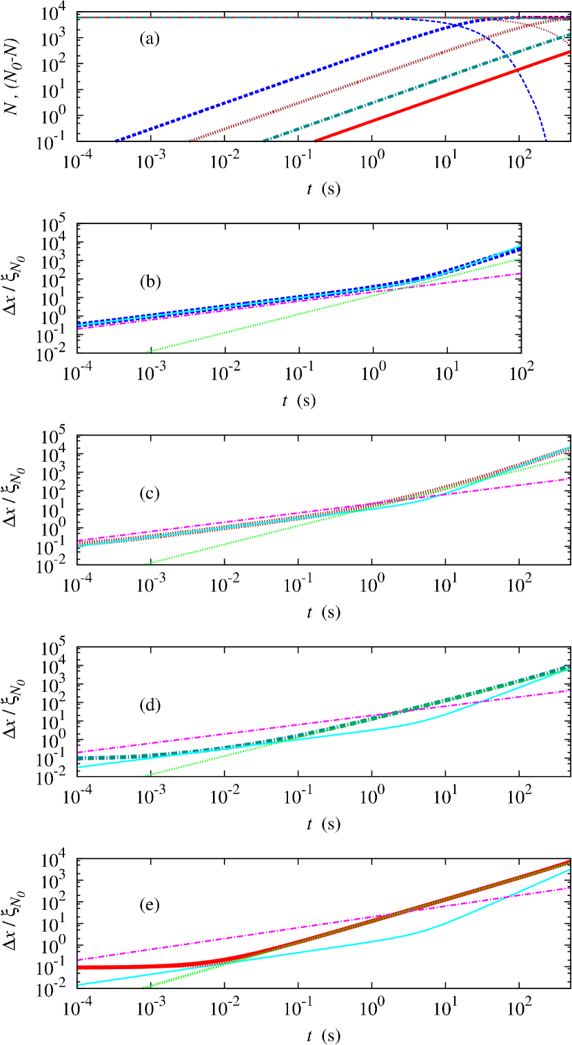
Figure 1: Li-bright soliton under the influence of single-particle losses (parameters as in footnote 4 but with $K_{3}=0$ and $N(0)=6000$). Panel a: particle number $N(t)$ (thin curves) and $N(0)-N(t)$ (thick curves). Thick blue (black) dashed curves correspond to a moderate vacuum with single particle losses given by $t_{1}=20\,\rm s$ (panel b), wide brown (black) short dashed curves an excellent vacuum $t_{1}=200\,\rm s$ (panel c), wide dark green (black) short dashed curves: $t_{1}=2000\,\rm s$ (panel d), wide red (black) solid curves: $t_{1}=10000\,\rm s$ (panel e). Thin light blue (gray) solid curves: analytical formula (32). As guides to the eye we added the magenta (dark gray) dash-dotted curves ($\propto\sqrt{t}$) and the green (light gray) dotted curves ($\propto t$). Data files are available online Weiss et al. (2015b).

Including the higher-order terms coming from the initial state (cf. Appendix B), Eq. (32) becomes (for not too large times)

$$(\Delta X)^{2}(t)\simeq\sigma_{X,0}^{2}+\frac{\sigma_{X}^{2}}{\langle\delta t\rangle}t+\sigma_{V,0}^{2}t^{2}+\frac{1}{3}\frac{\sigma_{V}^{2}}{\langle\delta t\rangle}t^{3}.$$ (38)

IV.3 Bright solitons in ⁷Li

As the comparison of the relevant time-scales (37) suggests Li as the more suitable candidate, we start with Li; Rb follows in Sec. IV.4.

In order to show the validity of the analytical approach we initially focus on single-particle losses (Fig. 1). For the parameters of the experiment of Ref. Khaykovich et al. (2002) (see footnote 4 but without three-particle losses), the analytical approach works very well even without the initial velocity. For the parameters used in Fig. 1 the initial velocity only plays an important role for idealized small values for single particle losses. Superballistic behavior is particularly well visible for less perfect vacuum.

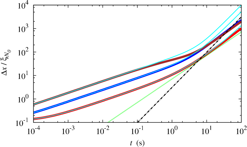
Figure 2: Root-mean-square fluctuation of the spreading of the center-of-mass density of a Li-bright soliton as a function of time. Thick curves: numerical data from Fig. 3 of Ref. Weiss et al. (2015a); the agreement is good for not too large times. Light blue (dark gray) curves: analytical formula (38). Superballistic spreading of the center-of-mass density is barely visible in the numerics and by far not as strong as predicted by the analytical approach. Data files are available online Weiss et al. (2015b).

In Fig. 2 we focus on the dominant three-particle losses as done in Ref. Weiss et al. (2015a), the initial velocity again only plays a role for some of the parameters. Superballistic spreading of the center-of-mass density is well visible in the analytical curves but only barely visible in the numerics. This clearly indicates that our assumption that the loss rate is constant is not fulfilled. Nevertheless, the analytical equations provide a qualitative understanding for the dynamics.

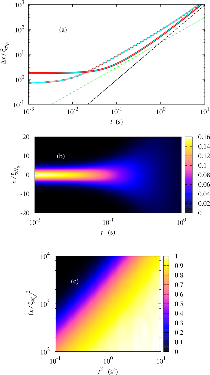
Figure 3: Superballistic spreading of the center-of-mass density for ⁷Li using the parameters of footnote 7 with $N(0)=100$ and a moderate vacuum with $t_{1}=20\,\rm s$. (a) Root-mean-square fluctuations of the center-of-mass as a function of time. Thick brown (black) dashed curve: computer-simulation if the initial harmonic oscillator length is 10 soliton lengths. Thick red/black solid curve: weaker initial trap (factor $2.5$ greater harmonic oscillator length) leads to clearly visible superballistic spreading of the center-of-mass density starting earlier. Light blue/light gray dashed and solid curves: corresponding analytical curves (38). As guides to the eye we added the green (light gray) dotted curve ($\propto t$) and the black dash-dotted curve ($\propto t^{3/2}$). (b) Two-dimensional projection of the single particle density (which is the convolution of the center-of-mass density and the soliton width) as a function of both time and position. This quantity is experimentally accessible by averaging over the positions of all particles, however it is insightful to plot it differently: by normalizing the maximum to one for each time shown [panel (c)]: Plotting the variance as a function of time squared shows again that the spreading occurs faster than ballistically (which would be parallel to the main diagonal in this panel). Data files are available online Weiss et al. (2015b).

Unfortunately, superballistic behavior starts rather late. In order to change this, we propose to use the parameters suggested in Ref. Weiss and Castin (2009). If the value of the initial trap has a harmonic oscillator length $\sqrt{\hbar/(m\omega)}$ that is 10 larger than the soliton length $\xi_{N}$ (the value used in all other figures), Fig. 3, primarily shows ballistic spreading of the center-of-mass density. However, as predicted by the analytical approach (38), using an initial trap for which the harmonic oscillator length is $25$ soliton lengths, superballistic spreading of the center-of-mass density becomes clearly visible already at short time-scales.

IV.4 Bright solitons in ⁸⁵Rb

Let us start by comparing the time-scales for Li and Rb bright solitons using the parameters in footnotes 4 and 5, based on the experiments of Refs. Khaykovich et al. (2002) and Marchant et al. (2013), Eqs. (35) and (36). Figure 4 confirms that Rb-bright solitons are less useful to investigate superballistic spreading of the center-of-mass density than Li-bright solitons if one uses the experimental parameters of Refs. Khaykovich et al. (2002) and Marchant et al. (2013): even if we chose an excellent vacuum, superballistic spreading of the center-of-mass density is not observable as too many particles are lost already.

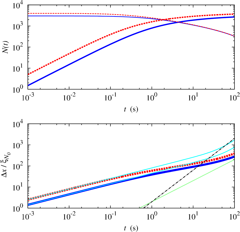
Figure 4: Rb-bright solitons under the influence of three-, two- and single-particle losses. Most parameters used can be found in footnote 5, additionally a very good vacuum with $t_{1}=200\,\rm s$ was chosen. Upper panel: red (black) dashed curves correspond to $N_{0}=4000$, blue (black) solid curves correspond to $N_{0}=3000$. Thin curves: $N(t)$; thick curves: $N_{0}-N(t)$. Lower panel: Root-mean-square fluctuations of the center-of-mass position. Red (black) dashed curves correspond to $N_{0}=4000$, blue (black) solid curves correspond to $N_{0}=3000$. Light blue (light gray) solid curves: analytical curves that assume the time $\langle\delta t\rangle$ for one loss event remains constant [Eq. (38)]. As guides to the eye for ballistic motion a curve $\propto t$ [green (light gray) dotted line] and a curve $\propto t^{3/2}$ for superballistic motion (black dash-dotted line) have been added. Data files are available online Weiss et al. (2015b).

However, even without changing the experimental parameters in future Rb-experiments as suggested in the lines below Eq. (37), performing such experiments can be very useful. Contrary to the case of Li, both two-particle and three-particle losses are present for Rb. If we assume that the values given in footnote 5 have an error of a factor of 5, this leads to quite distinct curves for the number of atoms as a function of time (Fig. 5). Contrary to the experiment of Ref. Roberts et al. (2000) for which two-particle losses are the dominant loss process, for the bright solitons investigated experimentally in Marchant et al. (2013) both loss rates are initially comparable. The effects of single particle losses would have to be included only for a very much smaller error margin.

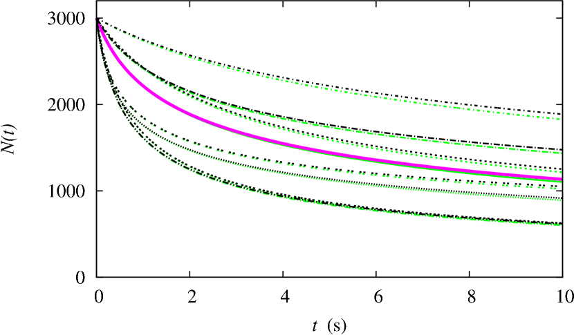
Figure 5: Number of atoms in a Rb-bright solitons under the influence of three-, two- and single-particle losses for $N=3000$ and the parameters given in footnote 5. Thick magenta (dark gray) line: parameters as in footnote 5. Thin black lines: an error of a factor of 5 was added to the loss parameters. Green (light gray) lines: also includes single-particle losses with $t_{1}=200\,\rm s$. All data generated with analytical equations map [cf. Eqs. (21) and (22)]; the numerical data from Fig. 4 lies on top of the corresponding green curve in this figure (which in turn is partially identical to the thick magenta (dark gray) curve). Data files are available online Weiss et al. (2015b).

If, on the other hand, we go the path of changing the parameters in the Rb-experiments Marchant et al. (2013, 2016), one approach would be to choose deep optical lattices perpendicular to the quasi-one-dimensional wave guide which would allow trapping frequencies in the kHz regime. Implementing optical lattices might even provide the possibility of having many tubes in which a very similar experiment is performed, thus allowing to average over different realizations of the spreading of the center-of-mass density in a single experiment.

For Fig. 6, we use the parameters of footnote 5 except for $\omega_{\perp}=2\pi\times 0.972\,\rm kHz$. This increase of the trapping frequency by a factor of 36 reduces the perpendicular harmonic oscillator length only by a factor of 6 while reducing the soliton length (4) via Eq. (2) by a factor of 36 (if $N$ remains of the order of 6000 atoms). While this endangers the one-dimensional character of our wave guide, this can easily be compensated by reducing the particle numbers. We thus reduce the particle number. When doing this, we also have to ensure that $10\times t^{*}/\langle\delta t\rangle\ll N_{0}$ is fulfilled (to be in the regime of weak decoherence even after superballistic spreading of the center-of-mass density has set in, thus we have to fulfill [cf. Eqs. (14), (17), (33) and (24)]

$$10t^{*}\left({\frac{1}{t_{1}}+\frac{N^{2}}{2t_{2}}+\frac{N^{4}}{3t_{3}}}\right)\ll 1$$ (39)

The fact that three-body losses are larger for Rb than for Li (see footnotes 4 and 5) requires low particle numbers to make the second and third term small, as $t^{*}\propto\frac{1}{N}$, the first term then requires nearly perfect vacuum. As a proof of principle, Fig. 6 displays superballistic spreading of the center-of-mass density for a Rb-bright soliton. However, contrary to what we suspected in Ref. Weiss et al. (2015a) it is not the heavier mass of Rb that makes it less useful for experimental realizations — the analytic treatment leading to Eq. (39) shows that it is rather the higher loss rates. While the time-scale in Fig. 6 could easily be reduced by choosing higher particle numbers, two- and three- particle losses would then prevent us from observing superballistic spreading of the center-of-mass density in both computer simulations and experiments.

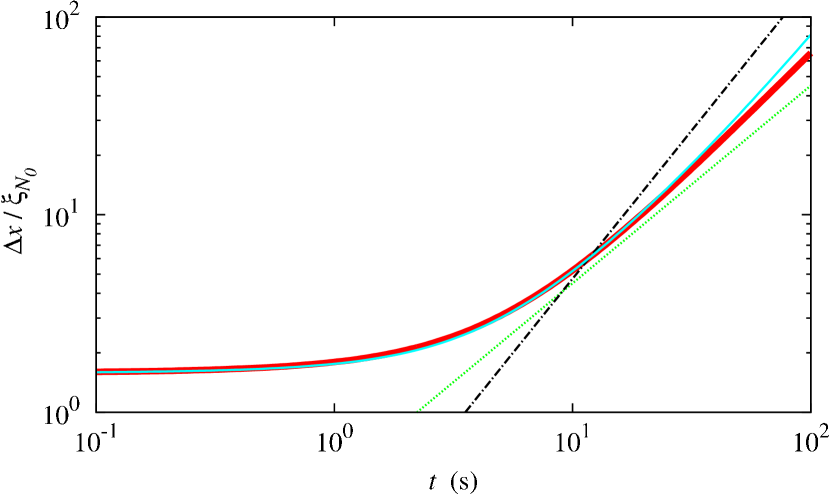
Figure 6: Superballistic spreading of the center-of-mass density in ⁸⁵Rb-bright solitons. The parameters are the same as in footnote 5 except for $\omega_{\perp}=2\pi\times 0.972\,\rm kHz$, the particle number is lower than in all other plots ($N=20$) and the vacuum is nearly perfect ($t_{1}=2000\,\rm s$). As for nearly all other curves, the initial trap is a factor of 10 larger than the soliton length. While the numerics [thick red (black) curve] does not reach the $\propto t^{3/2}$ behavior (black dash-dotted curve), predicted by the analytical approach [light blue (light gray) solid line; Eq. (38)] it does grow faster than $\propto t$ [green (light gray) dotted line]. Data files are available online Weiss et al. (2015b).

V Conclusion and outlook

To conclude, the main results of our paper treating attractively interacting Bosons in a quasi-one-dimensional waveguide with an additional initial weak harmonic trap are:

1. We present an analytical solution for the numerical model of the spreading of the center-of-mass density introduced in Ref. Weiss et al. (2015a) under the influence of decoherence via single- two- or three-body losses.

2. For stronger decoherence, the analytical model still qualitatively describes the transition from short-time diffusive to long-time ballistic behavior investigated numerically in Ref. Weiss et al. (2015a) (Figs. 2 and 4).

3. The analytical solutions predict center-of-mass rms fluctuations as a function of time that scales as $\propto t^{3/2}$; in the numerics the scaling is slower but still considerably faster than the ballistic ($\propto t$) regime (Figs. 3 and 6).

4. For ⁸⁵Rb, measuring the decay of the number of particles could furthermore help narrowing down the error margins for two- and three-particle losses (Fig. 5).

For many aspects of the spreading of the center-of-mass density ⁷Li-bright solitons are more suitable as, in particular, the time-scale for particle losses is longer. Our model differs considerably from the noise-driven motion of Ref. Maucher et al. (2012) and other systems used to investigate superballistic motion (see Zhao et al. (2014) and references therein): The decoherence-induced spreading of the center-of-mass density of quantum bright solitons described via the numerical model of Ref. Weiss et al. (2015a) can be viewed as a mesoscopic signature of microscopic quantum physics. The analytic solution presented here allowed us to predict and subsequently numerically observe superballistic motion.

Decoherence via particle losses is also likely to affect predictions beyond the center-of-mass motion. Unless one uses the approach of Ref. Weiss and Castin (2009) to focus on experiments with time-scales shorter than the first decoherence-event, theoretical predictions for bright solitons are likely to change if decoherence via particle losses is included.

Topics for which this might play a role include interferometric applications Polo and Ahufinger (2013); Streltsova and Streltsov (2014); Helm et al. (2015) and modeling the collisions of two bright solitons observed recently in the experiment of Ref. Nguyen et al. (2014) (cf. Martin (2016)) — in particular as soon as beyond-mean field quantum effects play a role Holdaway et al. (2013) in these collisions. The long-time behavior of bright solitons after scattering from a barrier, investigated experimentally for a large repulsive barrier in Ref. Marchant et al. (2013) and for a narrow attractive barrier in Ref. Marchant et al. (2016), are likely to be affected.

The model introduced in Ref. Weiss et al. (2015a) and solved analytically in the current paper is based on the unique properties of quantum bright solitons. Developing a similar model valid for repulsive interactions is an interesting question for future research.

The data presented in this paper will be available online at http://dx.doi.org/10.15128/44558d350 Weiss et al. (2015b).

Appendix A Lieb-Linger model with attractive interactions

For attractively interacting atoms ($g_{\rm 1D}<0$) in one dimension, the Lieb-Liniger-(McGuire) Hamiltonian Lieb and Liniger (1963); McGuire (1964) is a very useful model

$$\hat{H}=-\sum_{j=1}^{N}\frac{\hbar^{2}}{2m}\frac{\partial^{2}}{\partial x_{j}^{2}}+\sum_{j=1}^{N-1}\sum_{n=j+1}^{N}g_{\rm 1D}\delta(x_{j}-x_{n});$$ (40)

$x_{j}$ denotes the position of particle $j$ of mass $m$. For this model, even the (internal) ground state wave function is known analytically. Including the center-of-mass momentum $K$, the corresponding eigenfunctions relevant for our dynamics read (cf. Castin and Herzog (2001))

$$\Psi(x_{1},x_{2},\ldots,x_{N})\propto e^{iKX}\exp\left(-\frac{m|g_{\rm 1D}|}{2\hbar^{2}}\sum_{j<\nu}|x_{j}-x_{\nu}|\right);$$ (41)

the center-of-mass coordinate is given by Eq. (6). If the center-of-mass wave function is a delta function and the particle number is $N\gg 1$, then the single-particle density can be shown Calogero and Degasperis (1975); Castin and Herzog (2001) to be equivalent to the mean-field result (3). Thus, the Lieb-Liniger model is a one-dimensional many-particle quantum model that can be used to justify the approach to treat a quantum bright soliton like a mean-field soliton with additional center-of-mass motion after opening a weak initial trap. In the limit $N\to\infty$, $g_{\rm 1D}\to 0$ such that $Ng_{\rm 1D}=\rm const$, the initial width of the center-of-mass wave function goes to zero, $\Delta X_{0}\propto 1/\sqrt{N}$.

Appendix B Deriving the analytic results

In order to derive an analytical expression for the variance of the position of the center of mass $X$ we use the approximation of a constant particle number $N$. The master equation (25) can then be written in the simpler form

$$\frac{\partial}{\partial t}P(X,V,t)= -V\frac{\partial}{\partial X}P(X,V,t)+\int dX^{\prime}\int dV^{\prime}W(X-X^{\prime},V-V^{\prime})P(X^{\prime},V^{\prime},t)-\Gamma P(X,V,t),$$ (42)

where $P(X,V,t)$ is the probability to find at time $t$ the center of mass coordinate $X$ and the velocity $V$. The rate for a transition $X\rightarrow X^{\prime}$, $V\rightarrow V^{\prime}$ is given by

$$W(X-X^{\prime},V-V^{\prime})=\Gamma\sqrt{\frac{1}{2\pi\sigma^{2}_{X}}}\exp\left({-\frac{(X-X^{\prime})^{2}}{2\sigma^{2}_{X}}}\right)\sqrt{\frac{1}{2\pi\sigma^{2}_{V}}}\exp\left({-\frac{(V-V^{\prime})^{2}}{2\sigma^{2}_{V}}}\right),$$ (43)

and the total transition rate takes the form

$$\Gamma=\Gamma^{(1)}+\Gamma^{{2}}+\Gamma^{(3)}=\frac{N}{t_{1}}+\frac{N^{3}}{2t_{2}}+\frac{N^{5}}{3t_{3}}=\langle\delta t\rangle^{-1}.$$ (44)

From the master equation (42) one can derive, without further approximations, the following equations of motion for the first and second moments of the process:

$$\frac{d}{dt}\langle X(t)\rangle = \langle V(t)\rangle,$$ (45)

$$\frac{d}{dt}\langle V(t)\rangle = 0,$$ (46)

$$\frac{d}{dt}\langle X^{2}(t)\rangle = 2\langle X(t)V(t)\rangle+\Gamma\sigma^{2}_{X},$$ (47)

$$\frac{d}{dt}\langle V^{2}(t)\rangle = \Gamma\sigma^{2}_{V},$$ (48)

$$\frac{d}{dt}\langle X(t)V(t)\rangle = \langle V^{2}(t)\rangle.$$ (49)

For example, to derive Eq. (45) one starts from

$$\langle X(t)\rangle=\int dX\int dVXP(X,V,t),$$ (50)

and takes the time derivative:

$$\frac{d}{dt}\langle X(t)\rangle=\int dX\int dVX\frac{\partial}{\partial t}P(X,V,t).$$ (51)

Substituting the master equation (42) leads to:

$$\frac{d}{dt}\langle X(t)\rangle=-\int dX\int dVXV\frac{\partial}{\partial X}P(X,V,t)+\int dX\int dV\int dX^{\prime}\int dV^{\prime}XW(X-X^{\prime},V-V^{\prime})P(X^{\prime},V^{\prime},t)-\Gamma\langle X(t)\rangle.$$ (52)

After partial integration the first term on the right-hand side yields $\langle V(t)\rangle$. Integrating first over $X$ and $V$ the second term gives $+\Gamma\langle X(t)\rangle$ which cancels out the third term. This leads to Eq. (45). In a similar way Eqs. (46) - (49) can be obtained.

The closed system of differential equations (45) - (49) for the moments can easily be solved to yield:

$$\langle X^{2}(t)\rangle-\langle X(t)\rangle^{2}= \sigma^{2}_{X,0}+\Gamma\sigma_{X}^{2}\;t+\sigma^{2}_{V,0}\;t^{2}+\frac{1}{3}\Gamma\sigma_{V}^{2}\;t^{3}$$

$$+2\Big{(}\langle X(0)V(0)\rangle-\langle X(0)\rangle\langle V(0)\rangle\Big{)}\,t,$$ (53)

where

$$\sigma^{2}_{X,0} =\langle X^{2}(0)\rangle-\langle X(0)\rangle^{2},$$ (54)

$$\sigma^{2}_{V,0} =\langle V^{2}(0)\rangle-\langle V(0)\rangle^{2}.$$ (55)

The last term on the right-hand side of Eq. (B) does not appear in the main text as it is zero because position and velocity are uncorrelated at the initial time.

Appendix C Random walk in velocity space

For a random-walk in velocity space Obukhov (1959); Baule and Friedrich (2006); Kessler and Barkai (2012) with Gaussian step-distribution characterized by

$$\sigma_{V} =\frac{\hbar}{2(N-3)m\sigma_{X}}$$ (56)

where

$$\sigma_{X} =\frac{\pi\xi_{N}}{\sqrt{3}}=\frac{\pi\hbar^{2}}{\sqrt{3}m|g_{\rm 1D}|(N-4)}$$ (57)

leads, for $(N-4)/(N-3)\simeq 1$, to an $N$- and particle-mass independent step-size:

$$\sigma_{V}=\frac{\sqrt{3}|g_{\rm 1D}|}{2\pi\hbar}\;.$$ (58)

For the velocity after $n$ random-walk steps we thus have:

$$(V)_{n}=\sum_{\ell=1}^{n}\delta V_{\ell}$$ (59)

For an $n$-independent time-step $\delta t$ (thus assuming $N\simeq N-n$), we have:

$$(\Delta X)^{2}_{n~{}V~{}\rm steps} \equiv\langle X(t)^{2}\rangle_{n~{}V~{}\rm steps}$$ (60)

$$=\rangle\left<\left(\sum_{\nu=1}^{n}V_{\nu}\right)\left(\sum_{\mu=1}^{n}V_{\mu}\right)\langle\delta t_{\mu}\delta t_{\nu}\rangle\right>_{n~{}V~{}\rm steps}$$

$$=\langle\delta t\rangle^{2}\sum_{\nu=1}^{n}\sum_{\mu=1}^{n}\sum_{\ell=1}^{\nu}\sum_{j=1}^{\mu}\left<\delta V_{\ell}\delta V_{j}\right>$$

$$=\langle\delta t\rangle^{2}\sum_{\nu=1}^{n}\sum_{\ell=1}^{\nu}\sum_{\mu=1}^{n}\sum_{j=1}^{\mu}\sigma_{V}^{2}\delta_{\ell,j}$$

$$=\langle\delta t\rangle^{2}\sigma_{V}^{2}\sum_{\nu=1}^{n}\sum_{\ell=1}^{\nu}\sum_{\mu=\ell}^{n}1.$$

Solving the remaining sums analytically yields map

$$(\Delta X)^{2}_{n~{}V~{}\rm steps} =\left(\frac{1}{3}{n}^{3}+\frac{1}{2}{n}^{2}+\frac{1}{6}n\right)\langle\delta t\rangle^{2}\sigma_{V}^{2}$$ (61)

$$\simeq\frac{1}{3}{n}^{3}\langle\delta t\rangle^{2}\sigma_{V}^{2}.$$ (62)

The above assumes that $\langle\delta t^{2}\rangle$ is $n$-independent; the $(\Delta X)^{2}\propto t^{3}$ dependence is visible because of $n\propto t$.

Appendix D Estimating the initial velocity

Figure 7 shows the importance of including the initial velocity: If the initial velocity is added to the analytical curves depicted in Fig. 1, this considerably increases the agreement between analytical and numerical results.

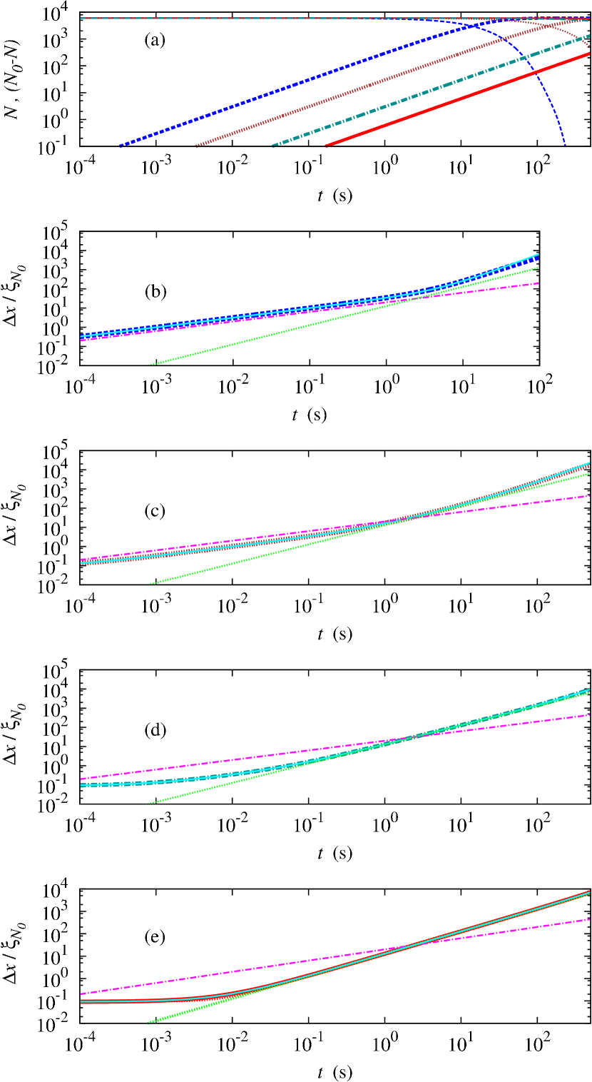
Figure 7: Li-bright soliton under the influence of single-particle losses (parameters as in footnote 4 but with $K_{3}=0$ and $N(0)=6000$). The data are the same as for Fig. 1 but for the fact that the analytical curves now include the initial velocity and the initial width of the wavepacket [Eq. (38)]. This leads to a much better agreement for weaker decoherence. Data files are available online Weiss et al. (2015b).

Comparing the very good agreement between analytical and numerical results if the correct value of the initial velocity is used (Fig. 7) to the approximation $\sigma_{V,0}=0$ (and $\sigma_{X,0}=0$) of Fig. 1 shows that the initial velocity does indeed play a role and merits our attention.

Particle losses are particularly easy to model if we have a product state. We start with a noninteracting Bose gas in the ground state of a one-dimensional harmonic trap; both in position space and in velocity space we have:

$$\sigma^{2}_{N}=\frac{\sigma^{2}_{1}}{N}$$ (63)

and this changes to

$$\sigma^{2}_{N-\nu}=\frac{\sigma^{2}_{1}}{N-\nu}$$ (64)

after one loss event losing $\nu$ particles, thus increasing the variance by

$$\widetilde{\sigma}^{2}=\sigma^{2}_{1}\left(\frac{1}{N-\nu}-\frac{1}{N}\right).$$ (65)

In order to estimate how long our assumption that the initial velocity distribution is given by Eq. (63) remains valid, we use a linear variation of the additional variance introduced in one step (65) during the ramping process

$$\sigma^{2}(t)=\widetilde{\sigma}^{2}+(\sigma^{2}_{\rm our~{}model}-\widetilde{\sigma}^{2})\frac{t}{T}.$$ (66)

For a specific experiment, we thus can check if

$$\frac{1}{\langle\delta t\rangle}\int_{0}^{T}\sigma^{2}(t)\ll\frac{\sigma^{2}_{1}}{N}$$ (67)

is indeed fulfilled. With $T$ typically in the tens of milliseconds Khaykovich (2015) for experiments like Khaykovich et al. (2002), $T/\langle\delta t\rangle\approx 50\,{\rm ms}/(200\,{\rm s}/N)$ if single-particle losses are the dominant source of decoherence during the adiabatic switching. For $N=6000$ we have less than 2 loss events and thus do not have to change the initial velocity in our model. The larger trapping frequencies for Li as compared to the heavier Rb leads to shorter switching times for Li. While this again is an argument for choosing lighter atoms for this type of experiment, future experiments are likely to show if further modeling is necessary.

References

- Zaburdaev et al. (2008) V. Zaburdaev, M. Schmiedeberg, and H. Stark, “Random walks with random velocities,” Phys. Rev. E 78, 011119 (2008).
- Zimbardo et al. (2000) G. Zimbardo, A. Greco, and P. Veltri, “Superballistic transport in tearing driven magnetic turbulence,” Physics of Plasmas 7, 1071 (2000).
- Prants et al. (2002) S. V. Prants, M. Edelman, and G. M. Zaslavsky, “Chaos and flights in the atom-photon interaction in cavity QED,” Phys. Rev. E 66, 046222 (2002).
- Liu and Bao (2014) Y. Liu and J. D. Bao, “Generation and application of non-ergodic noise,” Acta Physica Sinica 63, 240503 (2014).
- Levi et al. (2012) L. Levi, Y. Krivolapov, S. Fishman, and M. Segev, “Hyper-transport of light and stochastic acceleration by evolving disorder,” Nat. Phys. 8, 912 (2012).
- Hufnagel et al. (2001) L. Hufnagel, R. Ketzmerick, T. Kottos, and T. Geisel, “Superballistic spreading of wave packets,” Phys. Rev. E 64, 012301 (2001).
- Zhang et al. (2012) Y. Zhang, L. Mao, and C. Zhang, “Mean-field dynamics of spin-orbit coupled Bose-Einstein condensates,” Phys. Rev. Lett. 108, 035302 (2012).
- Stützer et al. (2013) S. Stützer, T. Kottos, A. Tünnermann, S. Nolte, D. N. Christodoulides, and A. Szameit, “Superballistic growth of the variance of optical wave packets,” Opt. Lett. 38, 4675 (2013).
- Zhao et al. (2014) Q. Zhao, C. A. Müller, and J. Gong, “Quantum and classical superballistic transport in a relativistic kicked-rotor system,” Phys. Rev. E 90, 022921 (2014).
- Weiss et al. (2015a) C. Weiss, S. A. Gardiner, and H.-P. Breuer, “From short-time diffusive to long-time ballistic dynamics: The unusual center-of-mass motion of quantum bright solitons,” Phys. Rev. A 91, 063616 (2015a).
- Khaykovich et al. (2002) L. Khaykovich, F. Schreck, G. Ferrari, T. Bourdel, J. Cubizolles, L. D. Carr, Y. Castin, and C. Salomon, “Formation of a matter-wave bright soliton,” Science 296, 1290 (2002).
- Strecker et al. (2002) K. E. Strecker, G. B. Partridge, A. G. Truscott, and R. G. Hulet, “Formation and propagation of matter-wave soliton trains,” Nature (London) 417, 150 (2002).
- Cornish et al. (2006) S. L. Cornish, S. T. Thompson, and C. E. Wieman, “Formation of bright matter-wave solitons during the collapse of attractive Bose-Einstein condensates,” Phys. Rev. Lett. 96, 170401 (2006).
- Marchant et al. (2013) A. L. Marchant, T. P. Billam, T. P. Wiles, M. M. H. Yu, S. A. Gardiner, and S. L. Cornish, “Controlled formation and reflection of a bright solitary matter-wave,” Nat. Commun. 4, 1865 (2013).
- Medley et al. (2014) P. Medley, M. A. Minar, N. C. Cizek, D. Berryrieser, and M. A. Kasevich, “Evaporative production of bright atomic solitons,” Phys. Rev. Lett. 112, 060401 (2014).
- McDonald et al. (2014) G. D. McDonald, C. C. N. Kuhn, K. S. Hardman, S. Bennetts, P. J. Everitt, P. A. Altin, J. E. Debs, J. D. Close, and N. P. Robins, “Bright solitonic matter-wave interferometer,” Phys. Rev. Lett. 113, 013002 (2014).
- Nguyen et al. (2014) J. H. V. Nguyen, P. Dyke, D. Luo, B. A. Malomed, and R. G. Hulet, “Collisions of matter-wave solitons,” Nat. Phys. 10, 918 (2014).
- Marchant et al. (2016) A. L. Marchant, T. P. Billam, M. M. H. Yu, A. Rakonjac, J. L. Helm, J. Polo, C. Weiss, S. A. Gardiner, and S. L. Cornish, “Quantum reflection of bright solitary matter waves from a narrow attractive potential,” Phys. Rev. A 93, 021604(R) (2016).
- Everitt et al. (2015) P. J. Everitt, M. A. Sooriyabandara, G. D. McDonald, K. S. Hardman, C. Quinlivan, M. Perumbil, P. Wigley, J. E. Debs, J. D. Close, C. C. N. Kuhn, and N. P. Robins, “Observation of Breathers in an Attractive Bose Gas,” ArXiv e-prints (2015), arXiv:1509.06844 [cond-mat.quant-gas] .
- Pethick and Smith (2008) C. J. Pethick and H. Smith, Bose-Einstein Condensation in Dilute Gases (Cambridge University Press, Cambridge, 2008).
- Baizakov et al. (2002) B. B. Baizakov, V. V. Konotop, and M. Salerno, “Regular spatial structures in arrays of Bose-Einstein condensates induced by modulational instability,” J. Phys. B 35, 5105 (2002).
- Al Khawaja et al. (2002) U. Al Khawaja, H. T. C. Stoof, R. G. Hulet, K. E. Strecker, and G. B. Partridge, “Bright soliton trains of trapped Bose-Einstein condensates,” Phys. Rev. Lett. 89, 200404 (2002).
- Hai et al. (2004) W. Hai, C. Lee, and G. Chong, “Propagation and breathing of matter-wave-packet trains,” Phys. Rev. A 70, 053621 (2004).
- Martin and Ruostekoski (2012) A. D. Martin and J. Ruostekoski, “Quantum dynamics of atomic bright solitons under splitting and recollision, and implications for interferometry,” New J. Phys. 14, 043040 (2012).
- Cuevas et al. (2013) J. Cuevas, P. G. Kevrekidis, B. A. Malomed, P. Dyke, and R. G. Hulet, “Interactions of solitons with a Gaussian barrier: splitting and recombination in quasi-one-dimensional and three-dimensional settings,” New J. Phys. 15, 063006 (2013).
- Polo and Ahufinger (2013) J. Polo and V. Ahufinger, “Soliton-based matter-wave interferometer,” Phys. Rev. A 88, 053628 (2013).
- Sun et al. (2014) Z.-Y. Sun, P. G. Kevrekidis, and P. Krüger, “Mean-field analog of the Hong-Ou-Mandel experiment with bright solitons,” Phys. Rev. A 90, 063612 (2014).
- Helm et al. (2015) J. L. Helm, S. L. Cornish, and S. A. Gardiner, “Sagnac interferometry using bright matter-wave solitons,” Phys. Rev. Lett. 114, 134101 (2015).
- Dunjko and Olshanii (2015) V. Dunjko and M. Olshanii, “Superheated integrability and multisoliton survival through scattering off barriers,” ArXiv e-prints (2015), arXiv:1501.00075 [cond-mat.quant-gas] .
- Lai and Haus (1989) Y. Lai and H. A. Haus, “Quantum theory of solitons in optical fibers. ii. exact solution,” Phys. Rev. A 40, 854 (1989).
- Drummond et al. (1993) P. D. Drummond, R. M. Shelby, S. R. Friberg, and Y. Yamamoto, “Quantum solitons in optical fibres,” Nature (London) 365, 307 (1993).
- Carr and Brand (2004) L. D. Carr and J. Brand, “Spontaneous soliton formation and modulational instability in Bose-Einstein condensates,” Phys. Rev. Lett. 92, 040401 (2004).
- Mishmash and Carr (2009) R. V. Mishmash and L. D. Carr, “Quantum entangled dark solitons formed by ultracold atoms in optical lattices,” Phys. Rev. Lett. 103, 140403 (2009).
- Streltsov et al. (2011) A. I. Streltsov, O. E. Alon, and L. S. Cederbaum, “Swift loss of coherence of soliton trains in attractive Bose-Einstein condensates,” Phys. Rev. Lett. 106, 240401 (2011).
- Fogarty et al. (2013) T. Fogarty, A. Kiely, S. Campbell, and T. Busch, “Effect of interparticle interaction in a free-oscillation atomic interferometer,” Phys. Rev. A 87, 043630 (2013).
- Delande et al. (2013) D. Delande, K. Sacha, M. Płodzień, S. K. Avazbaev, and J. Zakrzewski, “Many-body Anderson localization in one-dimensional systems,” New J. Phys. 15, 045021 (2013).
- Gertjerenken et al. (2013) B. Gertjerenken, T. P. Billam, C. L. Blackley, C. R. Le Sueur, L. Khaykovich, S. L. Cornish, and C. Weiss, “Generating mesoscopic Bell states via collisions of distinguishable quantum bright solitons,” Phys. Rev. Lett. 111, 100406 (2013).
- Barbiero et al. (2014) L. Barbiero, B. A. Malomed, and L. Salasnich, “Quantum bright solitons in the Bose-Hubbard model with site-dependent repulsive interactions,” Phys. Rev. A 90, 063611 (2014).
- Delande and Sacha (2014) D. Delande and K. Sacha, “Many-body matter-wave dark soliton,” Phys. Rev. Lett. 112, 040402 (2014).
- Krönke and Schmelcher (2015) S. Krönke and P. Schmelcher, “Many-body processes in black and gray matter-wave solitons,” Phys. Rev. A 91, 053614 (2015).
- Gertjerenken and Kevrekidis (2015) B. Gertjerenken and P.G. Kevrekidis, “Effects of interactions on the generalized Hong-Ou-Mandel effect,” Phys. Lett. A 379, 1737 (2015).
- Steinigeweg et al. (2007) R. Steinigeweg, H.-P. Breuer, and J. Gemmer, “Transition from diffusive to ballistic dynamics for a class of finite quantum models,” Phys. Rev. Lett. 99, 150601 (2007).
- Grabert et al. (1988) H. Grabert, P. Schramm, and G.-L. Ingold, “Quantum Brownian motion: The functional integral approach,” Phys. Rep. 168, 115–207 (1988).
- Jung and Hänggi (1991) P. Jung and P. Hänggi, “Amplification of small signals via stochastic resonance,” Phys. Rev. A 44, 8032 (1991).
- Lukić et al. (2005) B. Lukić, S. Jeney, C. Tischer, A. J. Kulik, L. Forró, and E.-L. Florin, “Direct observation of nondiffusive motion of a Brownian particle,” Phys. Rev. Lett. 95, 160601 (2005).
- Köppl et al. (2006) M. Köppl, P. Henseler, A. Erbe, P. Nielaba, and P. Leiderer, “Layer reduction in driven 2d-colloidal systems through microchannels,” Phys. Rev. Lett. 97, 208302 (2006).
- Hänggi and Marchesoni (2009) P. Hänggi and F. Marchesoni, “Artificial brownian motors: Controlling transport on the nanoscale,” Rev. Mod. Phys. 81, 387 (2009).
- Dierl et al. (2014) M. Dierl, W. Dieterich, M. Einax, and P. Maass, “Phase transitions in Brownian pumps,” Phys. Rev. Lett. 112, 150601 (2014).
- Turiv et al. (2015) T. Turiv, A. Brodin, and V. Nazarenko, “Anomalous Brownian motion of colloidal particle in a nematic environment: effect of the director fluctuations,” Condens. Matter Phys. 18, 23001 (2015).
- Fisher and Zwerger (1985) M. P. A. Fisher and W. Zwerger, “Quantum Brownian motion in a periodic potential,” Phys. Rev. B 32, 6190 (1985).
- Metzler and Klafter (2000) R. Metzler and J. Klafter, “The random walk’s guide to anomalous diffusion: a fractional dynamics approach,” Phys. Rep. 339, 1 (2000).
- Dür et al. (2002) W. Dür, R. Raussendorf, V. M. Kendon, and H.-J. Briegel, “Quantum walks in optical lattices,” Phys. Rev. A 66, 052319 (2002).
- Karski et al. (2009) M. Karski, L. Förster, J.-M. Choi, A. Steffen, W. Alt, D. Meschede, and A. Widera, “Quantum walk in position space with single optically trapped atoms,” Science 325, 174 (2009).
- Agliari et al. (2010) E. Agliari, A. Blumen, and O. Mülken, “Quantum-walk approach to searching on fractal structures,” Phys. Rev. A 82, 012305 (2010).
- Olshanii (1998) M. Olshanii, “Atomic scattering in the presence of an external confinement and a gas of impenetrable bosons,” Phys. Rev. Lett. 81, 938 (1998).
- Calogero and Degasperis (1975) F. Calogero and A. Degasperis, “Comparison between the exact and Hartree solutions of a one-dimensional many-body problem,” Phys. Rev. A 11, 265 (1975).
- Castin and Herzog (2001) Y. Castin and C. Herzog, “Bose-Einstein condensates in symmetry breaking states,” C. R. Acad. Sci. Paris, Ser. IV 2, 419 (2001), arXiv:cond-mat/0012040 .
- Lieb and Liniger (1963) E. H. Lieb and W. Liniger, “Exact Analysis of an Interacting Bose Gas. I. The General Solution and the Ground State,” Phys. Rev. 130, 1605 (1963).
- Castin (2009) Y. Castin, “Internal structure of a quantum soliton and classical excitations due to trap opening,” Eur. Phys. J. B 68, 317 (2009).
- Holdaway et al. (2012) D. I. H. Holdaway, C. Weiss, and S. A. Gardiner, “Quantum theory of bright matter-wave solitons in harmonic confinement,” Phys. Rev. A 85, 053618 (2012).
- Bonitz et al. (2007) M. Bonitz, K. Balzer, and R. van Leeuwen, “Invariance of the kohn center-of-mass mode in a conserving theory,” Phys. Rev. B 76, 045341 (2007).
- Flügge (1990) S. Flügge, Rechenmethoden der Quantentheorie (Springer, Berlin, 1990).
- Sinatra et al. (2002) A. Sinatra, C. Lobo, and Y. Castin, “The truncated Wigner method for Bose-condensed gases: limits of validity and applications,” J. Phys. B 35, 3599 (2002).
- Bienias et al. (2011) P. Bienias, K. Pawlowski, M. Gajda, and K. Rzazewski, “Statistical properties of one-dimensional attractive Bose gas,” EPL (Europhys. Lett.) 96, 10011 (2011).
- Davis (1993) M. H. A. Davis, Markov models and optimization (Chapman & Hall, London, 1993).
- Dalibard et al. (1992) J. Dalibard, Y. Castin, and K. Mølmer, “Wave-function approach to dissipative processes in quantum optics,” Phys. Rev. Lett. 68, 580 (1992).
- Dum et al. (1992) R. Dum, P. Zoller, and H. Ritsch, “Monte Carlo simulation of the atomic master equation for spontaneous emission,” Phys. Rev. A 45, 4879 (1992).
- Breuer and Petruccione (2006) H.-P. Breuer and F. Petruccione, The Theory of Open Quantum Systems (Clarendon Press, Oxford, 2006).
- Krönke et al. (2015) S. Krönke, J. Knörzer, and P. Schmelcher, “Correlated quantum dynamics of a single atom collisionally coupled to an ultracold finite bosonic ensemble,” New J. Phys. 17, 053001 (2015).
- Grimm et al. (2000) R. Grimm, M. Weidemüller, and Y. B. Ovchinnikov, “Optical Dipole Traps for Neutral Atoms,” Adv. At. Mol. Opt. Phys. 42, 95 (2000), physics/9902072 .
- (71) Computer algebra programme MAPLE, http://www.maplesoft.com/.
- Shotan et al. (2014) Z. Shotan, O. Machtey, S. Kokkelmans, and L. Khaykovich, “Three-body recombination at vanishing scattering lengths in an ultracold bose gas,” Phys. Rev. Lett. 113, 053202 (2014).
- Roberts et al. (2000) J. L. Roberts, N. R. Claussen, S. L. Cornish, and C. E. Wieman, “Magnetic field dependence of ultracold inelastic collisions near a Feshbach resonance,” Phys. Rev. Lett. 85, 728 (2000).
- Weiss et al. (2015b) C. Weiss, S. L. Cornish, S. A. Gardiner, and H.-P. Breuer, https://collections.durham.ac.uk/files/44558d350 and http://dx.doi.org/10.15128/44558d350 (2015b), “Superballistic center-of-mass motion in one-dimensional attractive Bose gases: Supporting Data”.
- Weiss and Castin (2009) C. Weiss and Y. Castin, “Creation and detection of a mesoscopic gas in a nonlocal quantum superposition,” Phys. Rev. Lett. 102, 010403 (2009).
- Maucher et al. (2012) F. Maucher, W. Krolikowski, and S. Skupin, “Stability of solitary waves in random nonlocal nonlinear media,” Phys. Rev. A 85, 063803 (2012).
- Streltsova and Streltsov (2014) O. I. Streltsova and A. I. Streltsov, “Interferometry with correlated matter-waves,” ArXiv e-prints (2014), arXiv:1412.4049 [quant-ph] .
- Martin (2016) A. D. Martin, “Collision-induced frequency shifts in bright matter-wave solitons and soliton molecules,” Phys. Rev. A 93, 023631 (2016).
- Holdaway et al. (2013) D. I. H. Holdaway, C. Weiss, and S. A. Gardiner, “Collision dynamics and entanglement generation of two initially independent and indistinguishable boson pairs in one-dimensional harmonic confinement,” Phys. Rev. A 87, 043632 (2013).
- Bowman et al. (2015) D. Bowman, P. Ireland, G. D. Bruce, and D. Cassettari, “Multi-wavelength holography with a single spatial light modulator for ultracold atom experiments,” Opt. Express 23, 8365 (2015).
- McGuire (1964) J. B. McGuire, “Study of Exactly Soluble One-Dimensional N-Body Problems,” J. Math. Phys. 5, 622 (1964).
- Obukhov (1959) A.M. Obukhov, “Description of turbulence in terms of lagrangian variables,” (Elsevier, 1959) p. 113.
- Baule and Friedrich (2006) A. Baule and R. Friedrich, “Investigation of a generalized obukhov model for turbulence,” Phys. Lett. A 350, 167 (2006).
- Kessler and Barkai (2012) David A. Kessler and Eli Barkai, “Theory of fractional lévy kinetics for cold atoms diffusing in optical lattices,” Phys. Rev. Lett. 108, 230602 (2012).
- Khaykovich (2015) L. Khaykovich, (2015), private communication.