Asymaptotic Scaling Laws of Wireless Adhoc Network with Physical Layer Caching

Abstract

We propose a physical layer (PHY) caching scheme for wireless adhoc networks. The PHY caching exploits cache-assisted multihop gain and cache-induced dual-layer CoMP gain, which substantially improves the throughput of wireless adhoc networks. In particular, the PHY caching scheme contains a novel PHY transmission mode called the cache-induced dual-layer CoMP which can support homogeneous opportunistic CoMP in the wireless adhoc network. Compared with traditional per-node throughput scaling results of $\Theta\left(1/\sqrt{N}\right)$, we can achieve $O(1)$ per node throughput for a cached wireless adhoc network with $N$ nodes. Moreover, we analyze the throughput of the PHY caching scheme for regular wireless adhoc networks and study the impact of various system parameters on the PHY caching gain.

I Introduction

Recently, wireless caching has been proposed as a cost-effective solution to handle the high traffic rate caused by content delivery applications [1, 2]. By exploiting the fact that content is “cachable”, wireless nodes can cache some popular content during off-peak hours (cache initialization phase), in order to reduce traffic rate at peak hours (content delivery phase). Caching has been widely used in wired networks such as fixed line P2P systems [3] and content distribution networks (CDN) [4]. One key difference between wireless and wired networks is that the performance of wireless networks is fundamentally limited by the interference. However, this unique feature of wireless networks is not fully exploited in existing wireless caching schemes. Recently, more advanced interference mitigation techniques such as coordinated multipoint (CoMP) transmission [5] have been proposed. Conventionally, the CoMP technique requires high capacity backhaul for payload exchange between the transmitting nodes. However, backhaul connectivity to the transmitting node may not be available in situations such as wireless adhoc networks. An interesting question is that, can we exploit wireless caching to achieve CoMP gain in wireless adhoc networks without payload backhaul connections between the nodes?

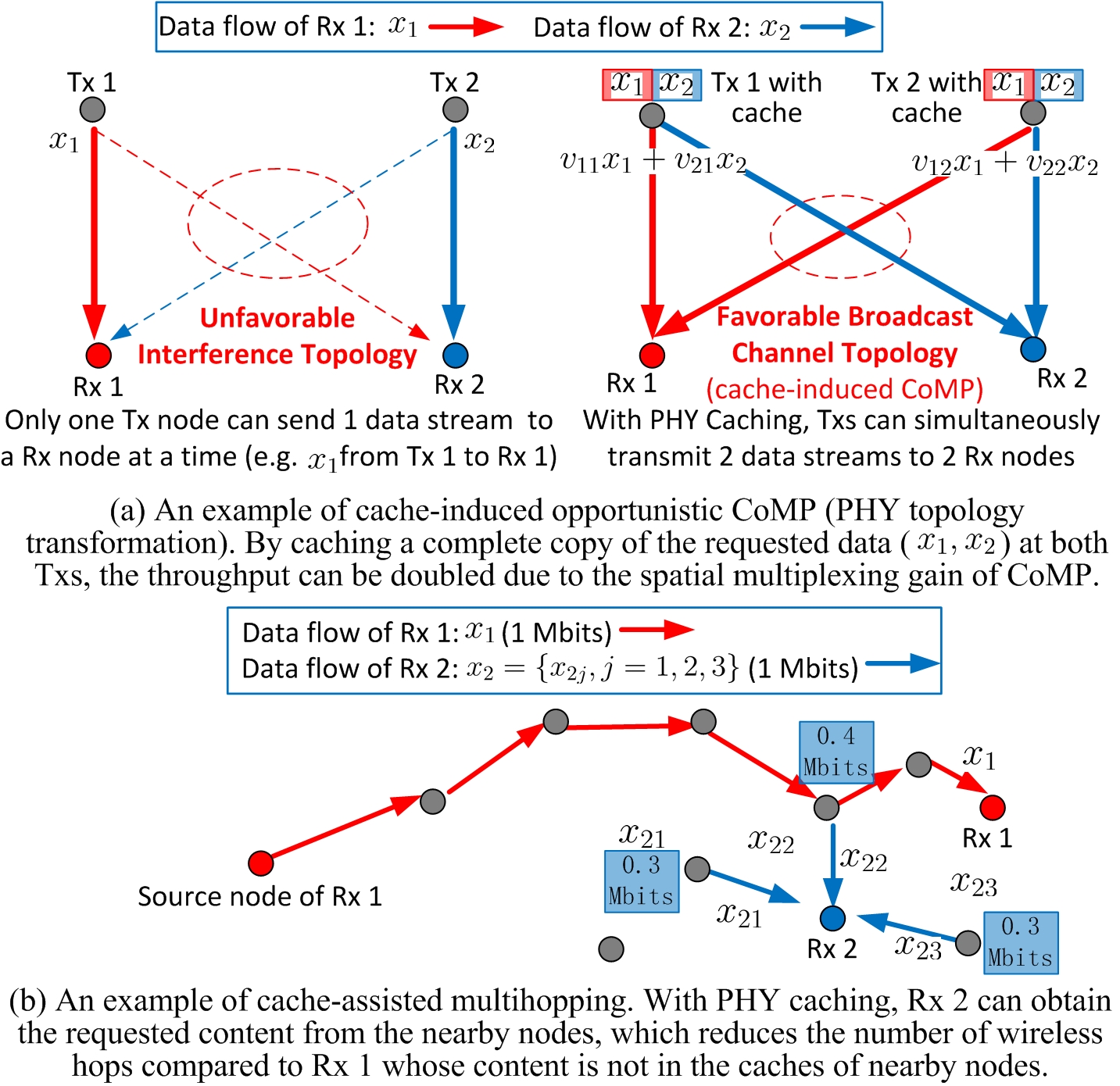
Figure 1: An illustration of cache-induced opportunistic CoMP and cache-assisted multihopping. In Fig. 1-(a), $\mathbf{v}_{1}=\left[v{}_{11},v_{12}\right]^{T}$ and $\mathbf{v}_{2}=\left[v{}_{21},v_{22}\right]^{T}$ are the beamforming vectors for Rx 1 and Rx 2, respectively.

In this paper, we propose a PHY caching scheme to achieve both cache-induced opportunistic CoMP and cache-assisted multihopping in wireless adhoc network as elaborated below.

• Cached-induced opportunistic CoMP: If the content accessed by several nodes exists simultaneously at the nearby nodes (i.e., each nearby node has a complete copy of the requested content), the nearby nodes can engage in CoMP and enjoy CoMP gain. In this way, we can opportunistically transform the interference network topology into a more favorable MIMO broadcast channel topology, as illustrated in Fig. 1-(a), and this is referred to as cache-induced opportunistic CoMP.

• Cached-assisted multihopping: If the content requested by a node is distributed in the caches of several nearby nodes (i.e., each nearby node has a different portion of the requested content), this node can directly obtain the requested content from the nearby nodes, which will significantly reduce the number of hops from the source nodes to the destination node, as illustrated in Fig. 1-(b). This is referred to as cache-assisted multihopping.

We are interested in studying the benefits of PHY caching and its impact on the throughput scaling law of cache-assisted wireless adhoc networks. Some related works are reviewed below. [6] proposed coded caching schemes that can create coded multicast opportunities. A proactive caching paradigm was proposed in [7] to exploit both the spatial and social structure of the wireless networks. [8] studied the joint optimization of cache content replication and routing in a regular network and identified the throughput scaling laws for various regimes. Recently, a number of works have studied the fundamental tradeoff or scaling laws in wireless device-to-device (D2D) caching networks [9, 10, 11, 12, 13]. For example, [9] investigated the fundamental limits of distributed caching in D2D wireless networks and the combined effect of coded multicast gain and spatial reuse. [10] characterized the optimal throughput-outage tradeoff in D2D caching networks in terms of tight scaling laws for various regimes. [11] presented a tutorial for the schemes and the recent results on the throughput scaling laws of D2D caching networks. A stochastic geometry framework, which incorporates the effects of random distributed users, user clustering, fading channel and interference, was proposed in [12] to study the tradeoff between the fraction of video requests served through D2D and the average rate. Note that the scaling laws studied in the above works and in this paper are different in many aspects. First, the existing caching schemes do not consider cache-induced CoMP among the nodes. In this paper, the roles of PHY caching include both the cache-assisted multihopping and the cache-induced dual-layer CoMP. Second, many theoretical results on scaling laws in wireless caching networks are based on the simple “protocol model” [14, 10] without considering the effect of PHY channel. Although some existing works such as [12] considered PHY channel model, none of them studied the coupling between caching and PHY transmission. In our analysis, we consider both the effect of PHY channel model and the coupling between caching and PHY transmission (e.g., the PHY transmission modes in our design depend on the cache mode of the requested file). Note that the concept of cached-induced opportunistic CoMP was first introduced in our previous works [15, 16] for cellular networks. However, the cached-induced opportunistic CoMP schemes in [15, 16] cannot be directly applied to wireless adhoc networks where a node may serve both as a transmitter that provides content and a receiver that requests content. As a result, we propose a new cache-induced dual-layer CoMP to support cached-induced opportunistic CoMP in wireless adhoc networks. To the best of our knowledge, a complete understanding of the role of caching in wireless networks is still missing, especially for the inter-play between the cache-assisted multihop gain and the cache-induced CoMP gains. The main contributions of this paper are as follows.

• PHY Caching for Multihopping and CoMP Gains: We propose a PHY caching design to exploit both cache-assisted multihopping and cache-induced dual-layer CoMP in wireless adhoc networks.

• Closed-form Performance Analysis for a Regular Wireless Adhoc Network: We derive closed-form expression of the per node throughput for the regular wireless adhoc network defined in Section IV. As a comparison, we also analyze the performance of a baseline multihop caching scheme which only achieves cache-assisted multihop gain. We quantify the cache-induced dual-layer CoMP gain (i.e., the throughput gain of the proposed PHY caching over the multihop caching) and study the impact of various system parameters on the performance.

• Throughput Scaling of Cache-assisted Wireless Adhoc Network: Under Zipf popularity distribution [17, 18], we show that the per node throughput of the cache-assisted wireless adhoc network with $N$ nodes scales from $\Theta\left(1/\sqrt{N}\right)$ to $\Theta\left(1\right)$ depending on the Zipf parameter $\tau$ and cache size.

The rest of the paper is organized as follows. In Section II, we introduce the system model. The PHY caching scheme is elaborated in Section III. The performance analysis for the regular wireless adhoc network is given in Section IV. The throughput scaling law of the proposed PHY caching is derived in Section V for general cache-assisted wireless adhoc network. Some numerical results are presented in Section VI. The conclusion is given in VII. The key notations are summarized in Table I.

$l_{n}$	Index of the file requested by node $n$
$q_{l}$	Cache content replication variable for file $l$
$p_{l}$	Probability of requesting file $l$
$\mathcal{N}_{C}^{1}$ ($\mathcal{N}_{C}^{2}$)	The set of all layer 1 (2) CoMP Tx nodes
$\Omega\left(\mathbf{q}\right)$ ($\overline{\Omega}\left(\mathbf{q}\right)$)	The set of files with multihop (CoMP) cache mode
$W_{b}$ ($W_{c}$)	Bandwidth of multihop (each CoMP) band
$\mathcal{B}_{n}$	Source node set of node n
$\mathcal{G}_{1,j}^{\textrm{Tx}}$ ($\mathcal{G}_{1,j}^{\textrm{Rx}}$)	$j$-th layer 1 CoMP transmit (receive) cluster
$N_{c}$	CoMP cluster size
$\Gamma_{B}\left(\mathbf{q}\right)$ ($\Gamma_{A}\left(\mathbf{q}\right)$)	Per node throughput under multihop (PHY) caching

Table I: Key notations

II Cache-assisted Wireless Adhoc Network Model

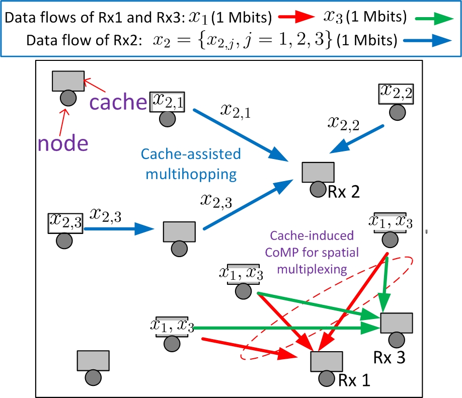
Figure 2: Architecture of the cache-assisted wireless adhoc network.

Consider a cache-assisted wireless adhoc network with $N$ nodes randomly placed on a square of area $Nr_{0}^{2}$ as illustrated in Fig. 2. Each node has an average transmit power budget of $P$ and a cache of size $B_{C}$ bits. We have the following assumption on the node placement.

Assumption 1 (Node Placement).

The node placement satisfies the following conditions.

1. The distance between any two nodes is no less than some constant $r_{\textrm{min}}>0$.

2. For any point in the square occupied by the network, the distance between this point and nearest node is no more than some constant $r_{\textrm{max}}>0$.

Assumption 1-1) is always satisfied in practice. Assumption 1-2) is to avoid the case when some nodes concentrate in a few isolated spots. Such case is undesired because a node in an isolated spot cannot be served whenever it requests content which is not in the caches of the nodes in the same spot.

In cache-assisted wireless adhoc network, the nodes request data (e.g., music or video) from a set of content files indexed by $l\in\mathcal{L}=\left\{1,2,...,L\right\}$. The size of the $l$-th file is $F_{l}$ bits and we assume $F_{l}=\Theta\left(B_{C}\right),\forall l$. There are two phases during the operation of cache-assisted wireless adhoc network, namely the cache initialization phase and the content delivery phase.

In the cache initialization phase, each node caches a portion of $q_{l}F_{l}$ (possibly encoded) bits of the $l$-th content file ($\forall l$) , where $\mathbf{q}=\left[q_{1},...,q_{L}\right]^{T}$ (with $q_{l}\in\left[0,1\right]$ and $\sum_{l=1}^{L}q_{l}F_{l}\leq B_{C}$) are called cache content replication vector. The specific cache data structure at each node and the algorithm to find $\mathbf{q}$ will be elaborated in Section III-B and Section V, respectively. Since the popularity of content files change very slowly (e.g., new movies are usually posted on a weekly or monthly timescale), the cache update overhead in the cache initialization phase is usually small [8]. This is a reasonable assumption widely used in the literature. However, the impact of “cache initialization phase” is worthy of further investigation, especially for the case when the popularity of content files changes more frequently.

In the content delivery phase, if the content requested by node $n$ is not in its own cache, it will obtain the requested content from a subset of other nodes that cache the requested content via cache-induced CoMP or cache-assisted multihopping. For example, in Fig. 2, the content accessed by Rx 1 and Rx 3 exists simultaneously at the cache of the nearby nodes and thus they can be served by the nearby nodes using cache-induced CoMP, enjoying spatial multiplexing gains. The content requested by Rx 2 is distributed in the caches of the nearby nodes and thus it is served by the nearby nodes using cache-assisted multihopping. For convenience, let $l_{n}$ denote the index of the file requested by node $n$ and let $\vec{l}=\left\{l_{1},...,l_{N}\right\}$ denote the user request profile (URP). The URP process $\vec{l}\left(t\right)$ is an ergodic random process. Specifically, each node independently accesses the $l$-th content file with probability $p_{l}$, where probability mass function $\mathbf{p}=\left[p_{1},...,p_{L}\right]$ represents the popularity of the content files.

We assume $B_{C}<\sum_{l=1}^{L}F_{l}$ to avoid the trivial case when each node can cache all content files. Furthermore, we assume $NB_{C}>\sum_{l=1}^{L}F_{l}$ so that there is at least one complete copy of each content file in the caches of the entire network. We use similar channel model as in [19, 20].

Assumption 2 (Channel Model).

The wireless link between two nodes is modeled by a flat block fading channel with bandwidth $W$. The channel coefficient between node $n$ and $n^{{}^{\prime}}$ at time slot $t$ is

$$h_{n^{{}^{\prime}},n}\left(t\right)=\left(r_{n^{{}^{\prime}},n}\right)^{-\alpha/2}\exp\left(j\theta_{n^{{}^{\prime}},n}\left(t\right)\right),$$

where $r_{n^{{}^{\prime}},n}$ is the distance between node $n$ and $n^{{}^{\prime}}$, $\theta_{n^{{}^{\prime}},n}\left(t\right)$ is the random phase at time $t$, and $\alpha>2$ is the path loss exponent. Moreover, $\theta_{n^{{}^{\prime}},n}\left(t\right)$ are i.i.d. (w.r.t. the node index $n^{{}^{\prime}},n$ and time index $t$) with uniform distribution on $\left[0,2\pi\right]$.

At each node, the received signal is also corrupted by a circularly symmetric Gaussian noise. Without loss of generality, the spectral density of the noise is normalized to be 1.

III PHY Caching for Wireless Adhoc Networks

We first outline the key components of the PHY caching scheme. Then we elaborate each component.

III-A Key Components of the PHY Caching Scheme

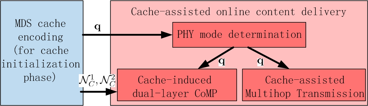
Figure 3: Components of PHY caching and their inter-relationship.

The components of the proposed PHY caching scheme and their inter-relationship are illustrated in Fig. 3. There are two major components: the maximum distance separable (MDS) cache encoding working in the cache initiation phase and the cache-assisted online content delivery working in the content delivery phase. The MDS cache encoding component converts the content files into coded segments and decides how to cache the coded segments at each node. The cache-assisted online content delivery component exploits the coded segments cached at each node to achieve both cache-induced CoMP gain and cache-assisted multihop gain. Specifically, there are two PHY transmission modes, namely, cache-assisted multihop transmission and cache-induced dual-layer CoMP transmission. At each node, a PHY mode determination component first determines the transmission mode. Then each node obtains the requested file using the corresponding transmission mode.

III-B Offline MDS Cache Encoding for Cache Initialization Phase

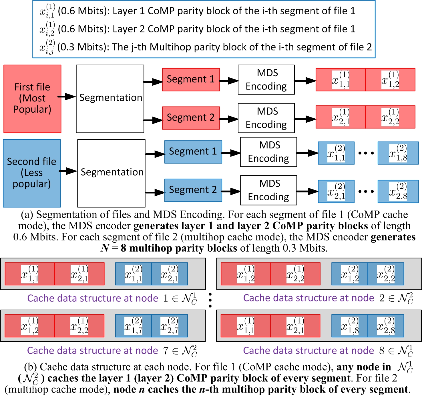
Figure 4: An illustration of MDS cache encoding. The network has $N=8$ nodes as shown in Fig. 5. There are $2$ content files with $q_{1}=0.6$ and $q_{2}=0.3$. The size of each file is $2$ Mbits and the segment size is $L_{S}=1$ Mbits. The cache size $B_{C}$ is 1.8 Mbits.

The cache-assisted multihopping and cache-induced dual-layer CoMP have conflicting requirements on the caching scheme. For the former, it is better to cache different content at different nodes so that the number of hops from the source to destination nodes can be minimized. For the later, the cache of the nearby transmitting nodes should store the same contents to support spatial multiplexing. Here, spatial multiplexing refers to simultaneous transmission of multiple data streams from a set of nearby serving nodes (which have the requested content in their caches) to a set of nearby requesting nodes using CoMP. We propose an MDS cache encoding scheme to strike a balance between these two conflicting goals.

MDS Cache Encoding Scheme (parameterized by a cache content replication vector $\mathbf{q}=\left[q_{1},...,q_{L}\right]^{T}$)

Step 1 (Nodes Partitioning): Partition the nodes into two non-overlapping subsets $\mathcal{N}_{C}^{1}$ and $\mathcal{N}_{C}^{2}$ using the following algorithm. First, node 1 marks itself as a node in $\mathcal{N}_{C}^{1}$ and broadcasts a MARK message containing a mark bit to the adjacent nodes. The mark bit is initialized to be bit 0. When a node receives a MARK message with SINR larger than a threshold $\gamma_{0}$ for the first time, if the mark bit is 0 (1), it marks itself as a node in $\mathcal{N}_{C}^{2}$ ($\mathcal{N}_{C}^{1}$ ) and sends a MARK message with mark bit 1 (0) to the adjacent nodes. After each node receives a MARK message (with SINR larger than $\gamma_{0}$) for at least once, the nodes have been partitioned into two non-overlapping subsets $\mathcal{N}_{C}^{1}$ and $\mathcal{N}_{C}^{2}$. The threshold $\gamma_{0}$ can be chosen according to the rules used in the existing neighbor discovery algorithms for wireless adhoc networks.

Step 2 (MDS Encoding and Cache Modes Determination): Each file is divided into segments of $L_{S}$ bits. Each segment is encoded using a MDS rateless code as shown in Fig. 4-(a). If $q_{l}\geq 0.5$, the cache mode for the $l$-th content file is set to be CoMP cache mode. In this case, for each segment of the $l$-th file, the MDS encoder first generates $2q_{l}L_{S}$ parity bits from the $L_{S}$ information bits of the original segment. Then the first $q_{l}L_{S}$ parity bits form the layer 1 CoMP parity block and the last $q_{l}L_{S}$ parity bits form the layer 2 CoMP parity block of this segment, as illustrated in Fig. 4-(a) for the first file. If $q_{l}<0.5$, the cache mode for the $l$-th content file is set to be multihop cache mode and the MDS encoder generates $N$ multihop parity blocks of length $q_{l}L_{S}$ for each segment of the $l$-th file as illustrated in Fig. 4-(a) for the second file. Define $\Omega\left(\mathbf{q}\right)\triangleq\left\{l:\>q_{l}<0.5\right\}$ as the set of files associated with multihop cache mode and $\overline{\Omega}\left(\mathbf{q}\right)\triangleq\left\{l:\>q_{l}\geq 0.5\right\}$ as the set of files associated with CoMP cache mode.

Step 3 (Offline Cache Initialization): For $l=1,..,L$, if $l\in\Omega\left(\mathbf{q}\right)$, then the cache of node $n$ is initialized with the $n$-th multihop parity block for each segment of the $l$-th file. If $l\in\overline{\Omega}\left(\mathbf{q}\right)$, then the caches of the nodes in $\mathcal{N}_{C}^{1}$ and $\mathcal{N}_{C}^{2}$ are initialized with the layer 1 and layer 2 CoMP parity blocks respectively.

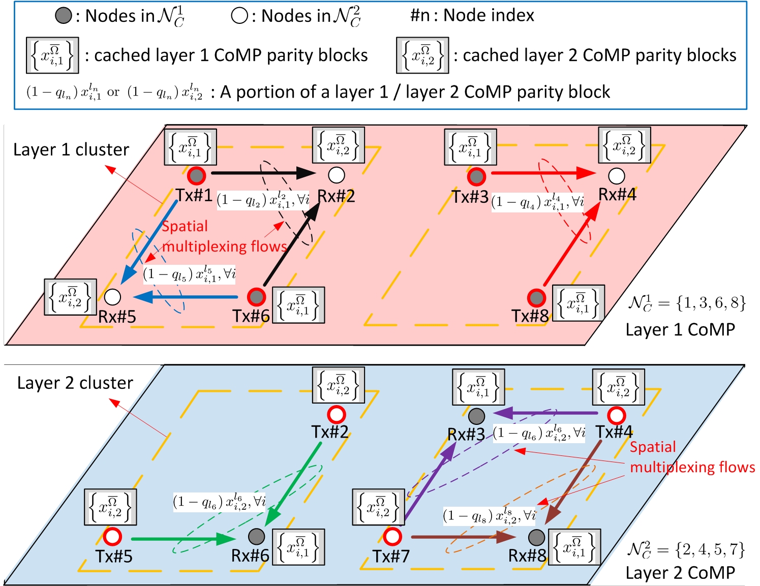
Figure 5: An illustration of cache-induced dual-layer CoMP, where each node in $\left\{2,3,4,5,6,8\right\}$ requests a file associated with CoMP cache mode.

The MDS cache encoding scheme has several benefits. First, the parity blocks of the requested segment can be received in any order without protocol overheads of reassembly due to the property of MDS codes. Second, when a node requests a file associated with multihop cache mode, it can always obtain the parity blocks required to decode this file from the nearest $\left\lceil 1/q_{l}\right\rceil-1$ nodes. Third, the introduction of CoMP cache mode for popular files facilitates the design of cache-induced dual-layer CoMP. To support homogeneous opportunistic CoMP in the wireless adhoc network, we propose a cache-induced dual-layer CoMP as illustrated in Fig. 5. Specifically, the nodes in the adhoc network are partitioned into two non-overlapping subsets $\mathcal{N}_{C}^{1}$ and $\mathcal{N}_{C}^{2}$ such that $\mathcal{N}_{C}^{1}\cap\mathcal{N}_{C}^{2}=\emptyset$ as illustrated in Step 1. The nodes in $\mathcal{N}_{C}^{1}$ ($\mathcal{N}_{C}^{2}$) cache the layer 1 (layer 2) CoMP parity blocks so that requesting nodes in $\mathcal{N}_{C}^{2}$ can be served with layer 1 CoMP transmission from nodes in $\mathcal{N}_{C}^{1}$, enjoying spatial multiplexing gains and vice versa for layer 2. For example, in Fig. 5, the nodes in $\mathcal{N}_{C}^{1}=\left\{1,3,6,8\right\}$ ($\mathcal{N}_{C}^{2}=\left\{2,4,5,7\right\}$) cache $\left\{x_{i,1}^{\overline{\Omega}}\right\}$ ($\left\{x_{i,2}^{\overline{\Omega}}\right\}$), which denotes the set of all layer 1 (2) parity blocks of all files $l\in\overline{\Omega}\left(\mathbf{q}\right)$ associated with the CoMP cache mode. The requesting nodes $2,4,5$ belong to $\mathcal{N}_{C}^{2}$ and thus they are served by the nodes in $\mathcal{N}_{C}^{1}=\left\{1,3,6,8\right\}$ using the layer 1 CoMP as illustrated in the red plane. The requesting nodes $3,6,8$ belong to $\mathcal{N}_{C}^{1}$ and thus they are served by the nodes in $\mathcal{N}_{C}^{2}=\left\{2,4,5,7\right\}$ using the layer 2 CoMP as illustrated in the blue plane.

The cache-assisted multihop gain and the cache-induced dual-layer CoMP gain depends heavily on the choice of the cache content replication vector $\mathbf{q}$. In Theorem 3, we will give an order-optimal cache content replication vector $\mathbf{q}$ to maximize the order of the per node throughput. The order-optimal $\mathbf{q}$ is calculated offline based on the content popularity $\mathbf{p}$.

III-C Frequency Planning for Interference Mitigation

The interference in adhoc networks is mitigated using the frequency planning technique. The bandwidth $W$ is divided into three bands, namely, the multihop band with size $W_{b}$ for the cache-assisted multihop transmission, the layer 1 CoMP band and the layer 2 CoMP band with size $W_{c}$ for the layer 1 and layer 2 CoMP transmissions respectively, where $W_{b}+2W_{c}=W$. As a result, these three transmissions can occur simultaneously without causing interference to each other. Furthermore, the multihop bandwidth $W_{b}$ is uniformly divided into $M$ subbands and each node is allocated with one subband such that the following condition is satisfied.

Condition 1 (Spatial reuse distance).

Any two nodes with distance no more than $r_{I}$ is allocated with different subbands, where $r_{I}>2r_{\textrm{max}}$ is a system parameter, and $r_{max}$ is defined in Assumption 1.

The following lemma gives the number of subbands that is required to satisfy the above condition.

Lemma 1 (Admissible frequency reuse factor).

There exists a frequency reuse scheme which has $M\leq\left(\frac{2r_{I}}{r_{\textrm{min}}}+1\right)^{2}+1$ subbands and satisfies Condition 1, where $r_{min}$ is the minimum distance between any two nodes as defined in Assumption 1.

Please refer to Appendix -A for the proof.

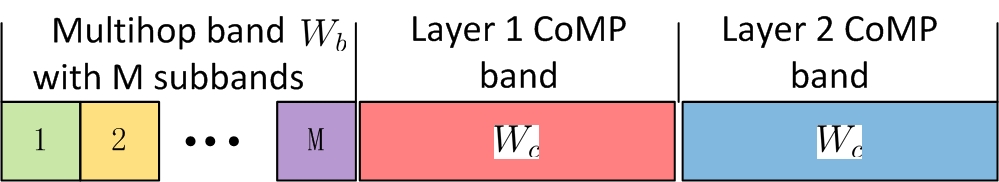
Figure 6: An illustration of the overall frequency planning scheme.

The overall frequency planning scheme is illustrated in Fig. 6. Note that in mobile adhoc networks, dynamic subband allocation (such as those studied in [21, 22]) is required for cache-assisted multihop transmission, where each node exchanges some information with the neighbor nodes and determines its multihop transmission subband dynamically to avoid strong interference.

Finally, we adopt uniform power allocation where the power allocated to each subband is proportional to the bandwidth of the subband. For example, at each node, the power allocated on the multihop subband is $\frac{W_{b}P}{W_{b}+MW_{c}}$ and the power allocated on the CoMP band is $\frac{MW_{c}P}{W_{b}+MW_{c}}$. The total transmit power of a node is given by $\frac{MW_{c}P}{W_{b}+MW_{c}}+\frac{W_{b}P}{W_{b}+MW_{c}}=P$.

III-D Online PHY Mode Determination

When node $n$ requests file $l_{n}$, it first determines the PHY mode. If $q_{l_{n}}<0.5$, node $n$ uses the cache-assisted multihop transmission to request file $l_{n}$; otherwise, it uses the cache-induced dual-layer Co-MIMO transmission. The PHY mode is fixed during the transmission of the entire file $l_{n}$.

III-E Online Cache-assisted Multihop Transmission

The cache-assisted multihop transmission for a node $n$ is summarized below.

Cache-assisted Multihop Transmission (for node $n$ requesting file $l_{n}$ with multihop cache mode)

Step 1 (Selection of Source Node Set $\mathcal{B}_{n}$ at node $n$)

1a (Request Broadcasting): Node $n$ broadcasts a REQ message which contains its position and the requested file index $l_{n}$ to the nodes which are no more than $r_{\textrm{RB}}=\left(2\sqrt{\left\lceil 1/q_{l_{n}}\right\rceil-1}+1\right)r_{\textrm{max}}$ away from node $n$. Specifically, if the distance between node $n^{{}^{\prime}}$ and node $n$ is larger than $r_{\textrm{RB}}$, node $n^{{}^{\prime}}$ will discard the REQ message from node $n$; otherwise, node $n^{{}^{\prime}}$ will 1) forward the REQ message to the neighbor nodes and 2) send an ACK message which contains its position to node $n$.

1b (Source Nodes Selection): Based on the ACK messages from the nearby nodes, node $n$ chooses the nearest nodes which have a total number of no less than $\left(1-q_{l_{n}}\right)L_{S}$ parity bits for each segment of the requested file $l_{n}$ as the source nodes. Specifically, let $r_{n}^{*}=\min\>r,\>\textrm{s.t. }\left|\left\{n^{{}^{\prime}}:\>r_{n,n^{{}^{\prime}}}\leq r\right\}\right|\geq\left\lceil 1/q_{l_{n}}\right\rceil$. Then the set of source nodes for node $n$ is given by $\mathcal{B}_{n}=\left\{n^{{}^{\prime}}\neq n:\>r_{n,n^{{}^{\prime}}}\leq r_{n}^{*}\right\}$.

1c (Load Partitioning): Node $n$ determines the load partitioning among the source nodes. Specifically, for each requested file segment, node $n$ will obtain $q_{l_{n}}L_{S}$ parity bits from each node in $\overline{\mathcal{B}}_{n}$ and $\frac{\left(1-q_{l_{n}}-\left|\overline{\mathcal{B}}_{n}\right|q_{l_{n}}\right)L_{S}}{\left|\mathcal{B}_{n}\right|-\left|\overline{\mathcal{B}}_{n}\right|}$ parity bits from each node in $\mathcal{B}_{n}\backslash\overline{\mathcal{B}}_{n}$, where $\overline{\mathcal{B}}_{n}=\left\{n^{{}^{\prime}}\neq n:\>r_{n,n^{{}^{\prime}}}<r_{n}^{*}\right\}$.

Step 2 (Multihop Routing and Transmission)

2a (Multihop Routing Path Establishment): For each source node $n^{{}^{\prime}}\in\mathcal{B}_{n}$, node $n$ sends a REQm message to node $n^{{}^{\prime}}$ to establish a multihop routing path between them. The REQm message contains the positions of node $n^{{}^{\prime}}$ and $n$, the requested file index $l_{n}$, and the number of requested parity bits per segment.

2b (Multihop Transmission): Each node $n^{{}^{\prime}}$ in $\mathcal{B}_{n}$ sends the requested parity bits as indicated by the REQm message to node $n$ along the multihop routing path established in step 2a. The source node set $\mathcal{B}_{n}$ and the multihop routing path are fixed during the transmission of the entire file $l_{n}$.

In step 1, the requesting node chooses the nearest nodes containing $\left(1-q_{l_{n}}\right)L_{S}$ multihop parity bits for each segment of the requested file $l_{n}$ as the source set $\mathcal{B}_{n}$. In step 2, the requesting node establishes the multihop routing path (route table) to and from the serving nodes in $\mathcal{B}_{n}$ using a geometry-based routing. Specifically, the coverage area is divided into $N$ Voronoi cells as illustrated in Fig. 7. Then the multihop routing path from node $n$ to node $n^{{}^{\prime}}$ consists of a sequence of hops along a routing line segment connecting node $n$ and node $n^{{}^{\prime}}$. In each hop, the REQm message (defined in step 2a) from node $n$ to node $n^{{}^{\prime}}$ are transferred from one Voronoi cell (node) to another in the order in which they intersect the routing line segment. For example, in Fig. 7, the routing line segment from node 1 to node 3 intersects cell 2 and cell 3. Then node 1 sends the REQm to node 3 via multihop transmission over the route “node 1$\rightarrow$node 2$\rightarrow$node 3”. The routing path from node $n^{{}^{\prime}}$ to $n$ can be obtained by reversing the routing path from node $n$ to $n^{{}^{\prime}}$. Note that each node on the routing path from node $n$ to node $n^{{}^{\prime}}$ can calculate the node index at the previous and the next hop based on the positions of node $n$ and node $n^{{}^{\prime}}$ in the REQm message, and the positions of the adjacent nodes. Hence, the route table at each node can be constructed in a distributed way using the position information in the REQm message. Finally, the requesting nodes obtain the multihop parity bits of the requested files from $\mathcal{B}_{n}$ via the established multihop routes. Together with the $q_{l_{n}}L_{S}$ parity bits of each segment stored at the local cache, node $n$ can decode each segment of file $l_{n}$.

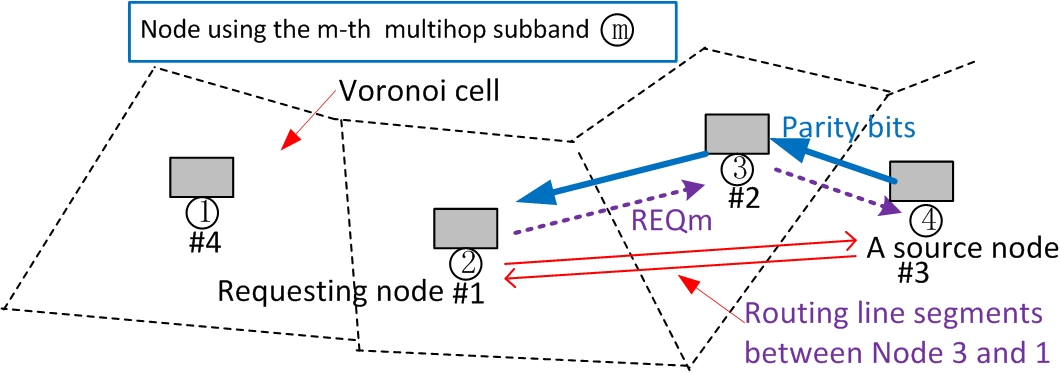
Figure 7: An illustration of multihop routing and transmission, where the requesting node 1 first sends REQm to a source node $3$ and then source node 3 sends the requested parity bits to node $1$.

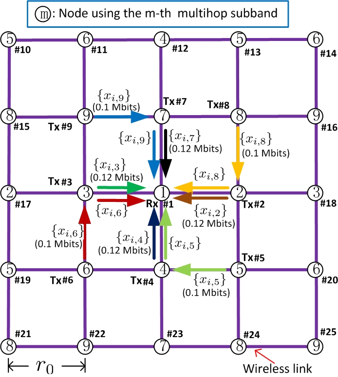
Figure 8: An illustration of cache-assisted multihop transmission in a regular wireless adhoc network, where node $1$ requests file $1$ associated with multihop cache mode. The $i$-th segment (with size $L_{S}=1$ Mbit) of file 1 is encoded into $N=25$ parity blocks of 0.12 Mbits and node $n$ caches the $n$-th parity block $x_{i,n}$ (0.12M parity bits).

Figure 7 illustrates a toy example of the overall cache-assisted multihop transmission. Node 1 requests file 1 of segment size $L_{S}=$1 Mbits using multihop mode. The source node set $\mathcal{B}_{1}=\left\{2,3,...,9\right\}$ determined by step 1 contains $0.96$M multihop parity bits. After step 2a, node 1 has established multihop paths to and from the source nodes $\left\{2,3,...,9\right\}$ as illustrated in Fig. 8. Then node 1 obtains $0.88$M parity bits for every segment of file 1 from nodes in $\mathcal{B}_{1}$ using multihop transmission. Together with the locally cached 0.12M parity bits for each segment of file 1, node 1 can decode file 1.

III-F Online Cache-induced Dual-layer CoMP Transmission

The cache-induced dual-layer CoMP transmission is illustrated in Fig. 5 and is summarized below.

Cache-induced Dual-layer CoMP Transmission

Step 1 (Dual-Layer CoMP Tx Node Clustering): Each CoMP layer $\mathcal{N}_{C}^{1}$ ($\mathcal{N}_{C}^{2}$) is further partitioned into CoMP clusters of size $N_{c}$ so that $\mathcal{N}_{C}^{1}=\cup_{j}\mathcal{G}_{1,j}^{\textrm{Tx}}$ and $\mathcal{N}_{C}^{2}=\cup_{j}\mathcal{G}_{2,j}^{\textrm{Tx}}$ . For example, in Fig. 5, we have $\mathcal{G}_{1,1}^{\textrm{Tx}}=\left\{1,6\right\}$, $\mathcal{G}_{1,2}^{\textrm{Tx}}=\left\{3,8\right\}$, $\mathcal{G}_{2,1}^{\textrm{Tx}}=\left\{2,5\right\}$ and $\mathcal{G}_{2,2}^{\textrm{Tx}}=\left\{4,7\right\}$.

Step 2 (Dual-Layer CoMP Rx Node Clustering): Suppose the requesting node $n\in\mathcal{N}_{C}^{2}$ . Each requesting node $n$ broadcasts the requested file index $l_{n}$ (associated with CoMP cache mode) to the nearest nodes in $\mathcal{N}_{C}^{1}$. The $j$-th CoMP cluster of layer 1 registers the requesting nodes and let $\mathcal{G}_{1,j}^{\textrm{Rx}}\subset\mathcal{N}_{C}^{2}$ be the set of all requesting nodes associated with the $j$-th layer 1 cluster $\mathcal{G}_{1,j}^{\textrm{Tx}}$. Fig. 5 illustrates an example in which $\mathcal{G}_{1,1}^{\textrm{Rx}}=\left\{2,5\right\}$, $\mathcal{G}_{1,2}^{\textrm{Rx}}=\left\{4\right\}$, $\mathcal{G}_{2,1}^{\textrm{Rx}}=\left\{6\right\}$ and $\mathcal{G}_{2,2}^{\textrm{Rx}}=\left\{3,8\right\}$.

Step 3 (CoMP transmission in each cluster): At each time slot, the nodes in $\mathcal{G}_{1,j}^{\textrm{Tx}}$ employ CoMP to jointly transmit the cached parity bits to the nodes in $\mathcal{G}_{1,j}^{\textrm{Rx}}$ simultaneously. On the other hand, node $n\in\mathcal{G}_{1,j}^{\textrm{Rx}}$ keeps receiving the requested portion of parity bits for each segment of file $l_{n}$ ($\left(1-q_{l_{n}}\right)L_{S}$ parity bits per segment) until all the requested segments of file $l_{n}$ is received. The CoMP transmission in the $j$-th layer 2 cluster is similar.

After clustering in step 1 and 2, the nodes in $\mathcal{G}_{1,j}^{\textrm{Tx}}$ and $\mathcal{G}_{1,j}^{\textrm{Rx}}$ forms a MISO broadcast channel topology with $N_{c}$ transmit antennas and $\left|\mathcal{G}_{1,j}^{\textrm{Rx}}\right|$ single receive antenna users as illustrated in Fig. 5, where the nodes in $\mathcal{G}_{1,1}^{\textrm{Tx}}=\left\{1,6\right\}$ forms a virtual transmitter with two distributed transmit antennas serving the two single antenna nodes in $\mathcal{G}_{1,1}^{\textrm{Rx}}=\left\{2,5\right\}$. The parity bits of the requested file segments for nodes in $\mathcal{G}_{1,j}^{\textrm{Rx}}$ can be transmitted simultaneously from the nodes in $\mathcal{G}_{1,j}^{\textrm{Tx}}$ using spatial multiplexing and therefore, the network throughput can be increased. Note that the serving nodes in $\mathcal{G}_{1,j}^{\textrm{Tx}}$ will transmit the same parity bits (codeword) to the same requesting node in $\mathcal{G}_{1,j}^{\textrm{Rx}}$. Let $\mathcal{C}_{1,j}\left(\left\{\mathbf{\Sigma}_{n},\sigma_{n}^{2}:n\in\mathcal{G}_{1,j}^{\textrm{Rx}}\right\}\right)$ denote the capacity region of the $j$-th layer 1 MISO BC (cluster) for a given set of transmit covariance matrices $\left\{\mathbf{\Sigma}_{n},\forall n\in\mathcal{G}_{1,j}^{\textrm{Rx}}\right\}$, where $\sigma_{n}^{2}=W_{c}+I_{n}^{c}$ is the variance of the effective noise at node $n$, and $I_{n}^{c}$ is the inter-cluster interference seen by node $n$. Then any rate tuple $\left(c_{n},\forall n\in\mathcal{G}_{1,j}^{\textrm{Rx}}\right)\in\mathcal{C}_{1,j}\left(\left\{\mathbf{\Sigma}_{n},\sigma_{n}^{2}:n\in\mathcal{G}_{1,j}^{\textrm{Rx}}\right\}\right)$ is achievable for the nodes in $\mathcal{G}_{1,j}^{\textrm{Rx}}$. The expression of $\mathcal{C}_{1,j}\left(\left\{\mathbf{\Sigma}_{n},\sigma_{n}^{2}:n\in\mathcal{G}_{1,j}^{\textrm{Rx}}\right\}\right)$ is well known (see e.g. [23]) and thus is omitted here for conciseness. Similarly, the $j$-th layer 2 cluster $\mathcal{G}_{2,j}^{\textrm{Tx}}$ and the associated nodes in $\mathcal{G}_{2,j}^{\textrm{Rx}}$ also form a MISO BC.

Remark 1.

In practice, it is difficult for each node to have global channel state information (CSI) for the entire network. Hence, we consider CoMP clustering so that each node only needs to know the local CSI within its cluster. In practice, we can allocate a dedicated control channel for each node to collect the local CSI. The CSI signaling usually consumes much less bandwidth compared to the data transmission because the former needs to be done on a per frame basis but the latter needs to be done on a per-symbol basis.

IV Throughput Analysis in Regular Wireless Adhoc Networks

In this section, we analyze the per node throughput of the proposed PHY caching scheme for regular wireless adhoc networks.

Definition 1 (Regular Adhoc Network).

In a regular wireless adhoc network, the $N$ nodes are placed on a grid as illustrated in Fig. 8. The distance between the adjacent nodes is $r_{0}$.

Similar to [8], we assume symmetric traffic model where all nodes have the same throughput requirement $R$ and all files have the same size, i.e., $F_{l}=F,\forall l$. To avoid boundary effects, we let $N\rightarrow\infty$. As a comparison, we will first analyze the performance of a baseline multihop caching scheme in which the PHY transmission scheme for all nodes is based on the cache-assisted multihop transmission summarized in Section III-E. After deriving closed form expressions of the per node throughput of both schemes, we will quantify the benefit of the proposed PHY caching scheme relative to the multihop caching scheme.

IV-A Per Node Throughput of Multihop Caching Scheme

In the multihop caching scheme, we set $r_{I}=2.5r_{0}$. As a result, the multihop bandwidth $W_{b}=W$ is divided into $M=9$ subbands as illustrated in Fig. 8. In Fig. 8, we also illustrate the cache-assisted multihop transmission scheme for a regular wireless adhoc network, where only two adjacent nodes can form a link and communicate with each other directly. First, we derive the average rate of each link.

Lemma 2.

In the cache-assisted multihop transmission, the average rate of each link is given by $WR_{b}$ (nats per second), where

$$R_{b}=\frac{1}{9}\log\left(1+\frac{9Pr_{0}^{-\alpha}}{W+9PI_{R}}\right),$$ (1)

$$I_{R} = \sum_{i=1}^{\infty}\frac{1}{r_{0}^{\alpha}}\left[\sum_{j=1}^{\infty}2\left(\left(3i+1\right)^{2}+9j^{2}\right)^{-\frac{\alpha}{2}}+\left|3i+1\right|^{-\alpha}\right]$$

$$+ \sum_{i=1}^{\infty}\frac{1}{r_{0}^{\alpha}}\left[\sum_{j=1}^{\infty}2\left(\left(3i-1\right)^{2}+9j^{2}\right)^{-\frac{\alpha}{2}}+\left|3i-1\right|^{-\alpha}\right]$$

$$+ \sum_{i=1}^{\infty}\frac{2}{r_{0}^{\alpha}}\left(9i^{2}+1\right)^{-\frac{\alpha}{2}}=\Theta\left(1\right).$$

Please refer to Appendix -B for the proof of Lemma 2. From Lemma 2, we obtain the achievable per node throughput in the following theorem.

Theorem 1 (Per node throughput of multihop caching).

Under the conventional multihop caching scheme, the per node throughput is

$$\Gamma_{B}\left(\mathbf{q}\right)=\frac{WR_{b}}{\sum_{l=1}^{L}p_{l}\psi\left(q_{l}\right)}.$$

where

$$\psi\left(q\right) = \frac{\phi\left(q\right)\left(1-q\right)-\frac{2}{3}\left(\phi^{3}\left(q\right)-\phi\left(q\right)\right)q}{2},$$ (2)

$$\phi\left(q\right) = \left\lceil\frac{-1+\sqrt{\frac{2}{q}-1}}{2}\right\rceil.$$

The intuition behind Theorem 1 is as follows. As can be seen in Fig. 8, for each node, the number of nodes with the nearest distance ($r_{0}$) from it is $4$, that with the second nearest distance ($\sqrt{2}r_{0}$) is $8$, and that with the $m$-th nearest distance is $4m$. Let $\mathcal{B}_{n,m}$ denote the set of nodes with the $m$-th nearest distance from node $n$. Suppose node $n$ requests the $l$-th file. Then $\phi\left(q_{l}\right)$ is the maximum number of hops between node $n$ and its source nodes in $\mathcal{B}_{n}$. For example, in Fig. 8, $q_{l}=0.12$ and thus the maximum number of hops between node $1$ and its source nodes is $\phi\left(0.12\right)=2$. It can be shown that the average traffic rate induced by a single node is $\sum_{l=1}^{L}p_{l}2\psi\left(q_{l}\right)R$, where $T_{l}\triangleq 2\psi\left(q_{l}\right)R$ is the traffic rate induced by a single node requesting the $l$-th file. Moreover, since the ratio between the number of links and the number of nodes is 2 as $N\rightarrow\infty$, the traffic rate on each link is $\sum_{l=1}^{L}p_{l}\psi\left(q_{l}\right)R$. Clearly, the per node throughput requirement $R$ can be satisfied if the traffic rate on each link does not exceed the average rate of each link, i.e., $\sum_{l=1}^{L}p_{l}\psi\left(q_{l}\right)R\leq WR_{b}$. Hence, the per node throughput is $\Gamma_{B}\left(\mathbf{q}\right)$. Please refer to Appendix -C for the detailed proof of Theorem 1.

IV-B Per Node Throughput of the Proposed PHY Caching Scheme

Recall that for $M=9$, the bandwidth of a multihop subband is $\frac{W-2W_{c}}{9}$ and the transmit power on this bandwidth is $\frac{\left(W-2W_{c}\right)P}{W+7W_{c}}$. The noise power is $\frac{W-2W_{c}}{9}$ and the interference power from the interfering nodes transmitting on the same multihop subband is $\frac{\left(W-2W_{c}\right)P}{W+7W_{c}}I_{R}$, where $I_{R}$ is given in Lemma 2. Hence the SINR of each link in the cache-assisted multihop transmission is $\frac{9Pr_{0}^{-\alpha}}{W+7W_{c}+9PI_{R}}$, and the corresponding rate is given by $\left(W-2W_{c}\right)R_{m}\left(W_{c}\right)$, where

$$R_{m}\left(W_{c}\right)=\frac{1}{9}\log\left(1+\frac{9Pr_{0}^{-\alpha}}{W+7W_{c}+9PI_{R}}\right).$$ (3)

Clearly, $R_{m}\left(W_{c}\right)$ is bounded as $R_{m}^{U}\geq R_{m}\left(W_{c}\right)\geq R_{m}^{L}$, where $R_{m}^{U}=R_{b}$ and

$$R_{m}^{L} = \frac{1}{9}\log\left(1+\frac{2Pr_{0}^{-\alpha}}{W+2PI_{R}}\right).$$

When a node requests a file with CoMP cache mode, it is served using the cache-induced dual-layer CoMP in Section III-F and the average rate has no closed-form expression. The following theorem gives closed-form bounds for the average rate in this case.

Theorem 2 (Average rate bounds for cache-induced dual-layer CoMP).

Let

$$G_{C}=\frac{4}{r_{0}^{\alpha}}\sum_{i=1}^{\infty}\sum_{j=1}^{\infty}\left[\left(\frac{\sqrt{2}}{2}+i\right)^{2}+\left(\frac{\sqrt{2}}{2}+j\right)^{2}\right]^{-\frac{\alpha}{2}}=\Theta\left(1\right)$$

$\rho=\frac{1}{2}\left(1-\frac{r_{0}^{-\alpha}}{G_{C}}\right)^{2}$, $R_{c}^{U}=\log\left(1+\frac{9PG_{C}}{W}\right)$ and $R_{c}^{L}=\rho\log\left(1+\frac{2Pr_{0}^{-\alpha}}{W}\right)$. The average rate of a node served using the cache-induced dual-layer CoMP is $W_{c}R_{c}\left(W_{c}\right)$, where $R_{c}\left(W_{c}\right)$ is bounded as

$$R_{c}^{U}\geq R_{c}\left(W_{c}\right)\geq R_{c}^{L}+O\left(PN_{c}^{-\frac{\alpha-2}{2\left(\alpha-1\right)}}\right).$$

In Theorem 2, the upper bound is obtained using the cut set bound between all nodes in $\mathcal{N}_{C}^{1}$ and a node in $\mathcal{N}_{C}^{2}$. The lower bound is obtained using an achievable scheme which ensures that the inter-cluster interference is negligible ($O\left(PN_{c}^{\frac{2-\alpha}{2\left(\alpha-1\right)}}\right)$ ) for large CoMP cluster size $N_{c}$. Then we can focus on studying the achievable sum rate of the MISO BC within each cluster. Finally, the lower bound can be derived from the achievable sum rate and the small term $O\left(PN_{c}^{-\frac{\alpha-2}{2\left(\alpha-1\right)}}\right)$ in the lower bound is due to the inter-cluster interference of order $O\left(PN_{c}^{\frac{2-\alpha}{2\left(\alpha-1\right)}}\right)$. Please refer to Appendix -D for the detailed proof.

Corollary 1 (Per node throughput bounds of PHY caching).

Under the proposed PHY caching scheme, the per node throughput $\Gamma_{A}\left(\mathbf{q}\right)$ is given by

$$\Gamma_{A}\left(\mathbf{q}\right)=\frac{WR_{m}\left(W_{c}^{*}\right)}{Q_{\Omega\left(\mathbf{q}\right)}+2Q_{\overline{\Omega}\left(\mathbf{q}\right)}R_{m}\left(W_{c}^{*}\right)/R_{c}\left(W_{c}^{*}\right)},$$ (4)

where $Q_{\Omega\left(\mathbf{q}\right)}=\sum_{l\in\Omega\left(\mathbf{q}\right)}p_{l}\psi\left(q_{l}\right)$, $Q_{\overline{\Omega}\left(\mathbf{q}\right)}=\sum_{l\in\overline{\Omega}\left(\mathbf{q}\right)}p_{l}\left(1-q_{l}\right)$, and $W_{c}^{*}$ is the unique solution of

$$Q_{\overline{\Omega}\left(\mathbf{q}\right)}\left(W-2W_{c}\right)R_{m}\left(W_{c}\right)=Q_{\Omega\left(\mathbf{q}\right)}W_{c}R_{c}\left(W_{c}\right).$$ (5)

Moreover, $\Gamma_{A}\left(\mathbf{q}\right)$ is bounded as $\Gamma_{A}^{U}\left(\mathbf{q}\right)\geq\Gamma_{A}\left(\mathbf{q}\right)\geq\Gamma_{A}^{L}\left(\mathbf{q}\right)+O\left(PN_{c}^{-\frac{\alpha-2}{2\left(\alpha-1\right)}}\right)$ with

$$\Gamma_{A}^{a}\left(\mathbf{q}\right)=\frac{WR_{m}^{a}}{Q_{\Omega\left(\mathbf{q}\right)}+2Q_{\overline{\Omega}\left(\mathbf{q}\right)}R_{m}^{a}/R_{c}^{a}},$$ (6)

for $a\in\left\{L,U\right\}$. Finally, as $P,N_{c}\rightarrow\infty$ such that $PN_{c}^{-\frac{\alpha-2}{2\left(\alpha-1\right)}}\rightarrow 0$, we have

$$\Gamma_{A}\left(\mathbf{q}\right)\rightarrow\frac{W}{9Q_{\Omega\left(\mathbf{q}\right)}}\log\left(1+\frac{r_{0}^{-\alpha}}{I_{R}}\right).$$ (7)

Please refer to Appendix -E for the proof. Note that the upper and lower bounds $\Gamma_{A}^{U}\left(\mathbf{q}\right),\Gamma_{A}^{L}\left(\mathbf{q}\right)$ are asymptotically tight at high SNR.

IV-C Order Optimal Cache Content Replication Solution

The per node throughput of both PHY caching and multihop caching is a non-concave function of the cache content replication vector $\mathbf{q}$. To make the analysis tractable, we aim at finding the order-optimal cache content replication solution. For convenience, the notation $N,L\overset{\xi}{\rightarrow}\infty$ refers to $N\rightarrow\infty$ and $\lim_{N\rightarrow\infty}\frac{L}{N}=\xi$. Since we assume $NB_{C}>LF$, we have $\xi\in\left[0,\frac{B_{C}}{F}\right)$. Note that $\xi$ is allowed to be zero. Hence as $N\rightarrow\infty$, $L$ can be either $\Theta\left(1\right)$ or go to infinity at an order no larger than $N$. The following corollary follows from Theorem 1 and Corollary 1. The detailed proof can be found in Appendix -F.

Corollary 2 (Per node throughput order in regular networks).

As $N,L\overset{\xi}{\rightarrow}\infty$, the per-node throughputs of the PHY caching and multihop caching schemes satisfy $\Gamma_{A}\left(\mathbf{q}\right)=\Theta\left(\frac{1}{\sum_{l=1}^{L}p_{l}\sqrt{\frac{1}{q_{l}}}}\right)$ and $\Gamma_{B}\left(\mathbf{q}\right)=\Theta\left(\frac{1}{\sum_{l=1}^{L}p_{l}\sqrt{\frac{1}{q_{l}}}}\right)$ respectively.

Consider the problem of maximizing the order of per node throughput in Corollary 2:

$$\min_{\mathbf{q}}\sum_{l=1}^{L}p_{l}\sqrt{\frac{1}{q_{l}}},\>s.t.\>q_{l}\in\left[\frac{1}{N},1\right],\forall l,\>\sum_{l=1}^{L}q_{l}\leq\frac{B_{C}}{F}.$$ (8)

The constraint $q_{l}\geq\frac{1}{N}$ is to ensure that there is at least one complete copy of the $l$-th file in the caches of the entire network. Problem (8) is convex and the optimal solution can be easily obtained using numerical method. To facilitate performance analysis, we characterize the order-optimal $\mathbf{q}$ in the following theorem. A cache content replication vector $\mathbf{q}$ is order-optimal for problem (8) if the achieved objective value is on the same order as the optimal objective value as $N,L\overset{\xi}{\rightarrow}\infty$. Note that the order-optimality here is w.r.t. problem (8) under the proposed scheme. It is not the order-optimality in information theoretic sense.

Theorem 3 (Order optimal cache content replication).

As $N,L\overset{\xi}{\rightarrow}\infty$, an order-optimal $\mathbf{q}$ is given by

$$q_{l}^{*}=\min\left(\left(\frac{B_{C}}{F}-\frac{L}{N}\right)\frac{p_{l}^{2/3}}{\sum_{l=1}^{L}p_{l}^{2/3}}+\frac{1}{N},1\right),\forall l.$$ (9)

Please refer to Appendix -G for the detailed proof. Theorem 3 implies that the order-optimal cache content replication variable $q_{l}$ is proportional to $p_{l}^{2/3}$, indicating that a larger portion of the cache capacity should be allocated to more popular content.

IV-D Benefits of PHY Caching

The PHY caching gain is defined as the throughput gap between the PHY caching and multihop caching. We analyze this gain under the Zipf content popularity distribution:

$$p_{l}=\frac{1}{Z_{\tau}\left(L\right)}l^{-\tau},l=1,...,L,$$ (10)

where the parameter $\tau$ determines the rate of popularity decline as $l$ increases, and $Z_{\tau}\left(L\right)=\sum_{l=1}^{L}l^{-\tau}$ is a normalization factor. The Zipf distribution is widely used to model the Internet traffic [17, 18]. The Zipf parameter $\tau$ usually ranges from 0.5 to 3 [18] depending on the application. Higher values of $\tau$ are usually observed in mobile applications [18]. Using Theorem 1 and Corollary 1, we can bound the PHY caching gain $\triangle\Gamma\triangleq\Gamma_{A}\left(\mathbf{q}^{*}\right)-\Gamma_{B}\left(\mathbf{q}^{*}\right)$ under the order-optimal cache content replication $\mathbf{q}^{*}$ in (9).

Corollary 3 (PHY caching gain).

The PHY caching gain is bounded as $\triangle\Gamma_{U}\geq\triangle\Gamma\geq\triangle\Gamma_{L}+O\left(PN_{c}^{-\frac{\alpha-2}{2\left(\alpha-1\right)}}\right)$ with

$$\triangle\Gamma_{a} = \Gamma_{A}^{a}\left(\mathbf{q}^{*}\right)-\Gamma_{B}\left(\mathbf{q}^{*}\right),$$ (11)

for $a\in\left\{L,U\right\}$. Moreover, as $P,N_{c}\rightarrow\infty$ such that $PN_{c}^{-\frac{\alpha-2}{2\left(\alpha-1\right)}}\rightarrow 0$, we have $\triangle\Gamma\rightarrow\overline{\triangle\Gamma}$, where

$$\overline{\triangle\Gamma} = \frac{W}{9}\log\left(1+\frac{r_{0}^{-\alpha}}{I_{R}}\right)\left(\frac{\sum_{l\in\overline{\Omega}\left(\mathbf{q}^{*}\right)}p_{l}\psi\left(q_{l}^{*}\right)}{Q_{\Omega\left(\mathbf{q}^{*}\right)}\sum_{l=1}^{L}p_{l}\psi\left(q_{l}^{*}\right)}\right)$$

$$= \Theta\left(\frac{\frac{B_{C}}{F}\sum_{l\in\overline{\Omega}\left(\mathbf{q}^{*}\right)}\left(1-q_{l}^{*}\right)}{\left[\sum_{l=1}^{L}p_{l}^{2/3}\right]^{3}}\right),$$

where $q_{l}^{*}$ is given in (9).

According to Corollary 3, the PHY caching gain can be well approximated by $\overline{\triangle\Gamma}$ at high SNR. Clearly, we have $\overline{\triangle\Gamma}\geq 0$. $\overline{\triangle\Gamma}$ captures the key features of the actual (simulated) PHY caching gain even at moderate SNR as illustrated in Fig. 9. From (3), we have the following observation about the impact of system parameters on $\overline{\triangle\Gamma}$.

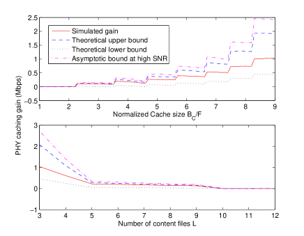
Figure 9: Impact of system parameters on the PHY caching gain in a regular wireless adhoc network with $N=512$ nodes. The system bandwidth is 1MHz and $\frac{Pr_{0}^{-\alpha}}{W}=10$dB. The content popularity skewness $\tau=$1. The CoMP cluster size is $N_{c}=9$. In the upper subplot, $L=12$. In the lower subplot, $B_{C}/F=2$.

Impact of the normalized cache size $\frac{B_{C}}{F}$: When $\frac{B_{C}}{F}<\left(0.5-\frac{1}{N}\right)\sum_{l=1}^{L}l^{-\frac{2}{3}\tau}+\frac{L}{N}$, we have $q_{l}^{*}<0.5,\forall l$ and $\overline{\triangle\Gamma}=0$. When $\frac{B_{C}}{F}=\left(0.5-\frac{1}{N}\right)\sum_{l=1}^{L}l^{-\frac{2}{3}\tau}+\frac{L}{N}$, $\overline{\triangle\Gamma}$ jumps from 0 to a positive value. As $\frac{B_{C}}{F}$ increases over the region $\left[\left(0.5-\frac{1}{N}\right)\sum_{l=1}^{L}l^{-\frac{2}{3}\tau}+\frac{L}{N},2^{\frac{2}{3}\tau}\left(0.5-\frac{1}{N}\right)\sum_{l=1}^{L}l^{-\frac{2}{3}\tau}+\frac{L}{N}\right)$, $\overline{\triangle\Gamma}$ keeps positive but its value may fluctuate. When $\frac{B_{C}}{F}=2^{\frac{2}{3}\tau}\left(0.5-\frac{1}{N}\right)\sum_{l=1}^{L}l^{-\frac{2}{3}\tau}+\frac{L}{N}$, $\overline{\triangle\Gamma}$ jumps to a larger value. As $\frac{B_{C}}{F}$ continues to increase, $\overline{\triangle\Gamma}$ repeats the pattern of fluctuations followed by a positive jump. Overall, $\overline{\triangle\Gamma}$ increases with $\frac{B_{C}}{F}$ as shown in the upper subplot of Fig. 9.

Impact of the number of content files $L$: In the lower subplot of Fig. 9, we plot $\overline{\triangle\Gamma}$ versus $L$ when fixing other parameters. It can be observed that $\overline{\triangle\Gamma}$ decreases with $L$. When $\tau\leq\frac{3}{2}$, there exists a large enough $L$, such that $\frac{B_{C}}{F}<\left(0.5-\frac{1}{N}\right)\sum_{l=1}^{L}l^{-\frac{2}{3}\tau}+\frac{L}{N}$ and $\overline{\triangle\Gamma}=0$.

Impact of the Content Popularity Skewness $\tau$: When $\tau>\frac{3}{2}$, $\sum_{l=1}^{L}p_{l}^{2/3}=\Theta\left(\sum_{l=1}^{L}l^{-\frac{2}{3}\tau}\right)$ is bounded and we can achieve a PHY caching gain of $\Theta\left(1\right)$ even when $L\rightarrow\infty$. On the other hand, when $\tau\leq\frac{3}{2}$, the normalized cache size $\frac{B_{C}}{F}$ has to increase with $L$ at the same order as $L\rightarrow\infty$ in order to achieve a PHY caching gain of $\Theta\left(1\right)$.

V Throughput Scaling Laws in General Wireless Adhoc Networks

In this section, we study throughput scaling laws for general wireless adhoc networks (i.e., the cache-assisted wireless adhoc networks described in Section II employing the proposed PHY caching scheme) as $N,L\overset{\xi}{\rightarrow}\infty$. We first give the order of the per node throughput of the proposed PHY caching scheme with fixed cache content replication $\mathbf{q}$.

Theorem 4 (Per node throughput order in general networks).

In a general cache-assisted wireless adhoc network with $N$ nodes, a per node throughput

$$R=\Theta\left(\frac{W}{M\sum_{l=1}^{L}p_{l}\sqrt{\frac{1}{q_{l}}}}\log\left(1+\frac{3MP\left(2r_{\textrm{max}}\right)^{-\alpha}}{\left(M+1\right)W+3MI_{A}}\right)\right)$$ (13)

can be achieved by the proposed PHY caching scheme with fixed cache content replication $\mathbf{q}$, where $M=\left(\frac{2r_{I}}{r_{\textrm{min}}}+1\right)^{2}+1$ and

$$I_{A}=\frac{4P\left(r_{I}-2r_{\textrm{max}}+r_{\textrm{min}}\right)}{r_{\textrm{min}}^{2}\left(r_{I}-2r_{\textrm{max}}\right)^{\alpha-1}}\left(\frac{2}{\alpha-2}+\frac{1}{\alpha-1}+3\right).$$

Please refer to Appendix -H for the proof.

The factor $\sum_{l=1}^{L}p_{l}\sqrt{\frac{1}{q_{l}}}$ in (13) is due to multihop transmission and it determines the order of per node throughput. When $q_{l}$ increases, the average number of hops from the source nodes to the destination nodes decreases and thus the order of per node throughput increases. Note that the order of the per node throughput in Theorem 4 is consistent with that of the regular wireless adhoc network in Corollary 2. Hence, the order optimal cache content replication solution in general wireless adhoc networks is also given by (9) in Theorem 3 and the following scaling laws follow straightforward from Theorem 3 and 4.

Corollary 4 (Asymptotic scaling laws of per node throughput).

Under the Zipf content popularity distribution in (10), the order optimal per node throughput in general wireless adhoc networks is given by $R^{*}=\Theta\left(\left[\sum_{l=1}^{L}p_{l}^{2/3}\right]^{-3/2}\right)$. Moreover, when $L=\Theta\left(1\right)$, we have $R^{*}=\Theta\left(1\right)$. When $N,L\rightarrow\infty$ and $\lim_{N\rightarrow\infty}\frac{L}{N}\in\left[0,\frac{B_{C}}{F}\right)$, we have

1. If $0\leq\tau<1$, $R^{*}=\Theta\left(1/\sqrt{L}\right)$.

2. If $\tau=1$, $R^{*}=\Theta\left(\log L/\sqrt{L}\right)$.

3. If $1<\tau<3/2$, $R^{*}=L^{\tau-3/2}$.

4. If $\tau=3/2$, $R^{*}=\log^{-3/2}L$.

5. If $\tau>3/2$, $R^{*}=\Theta\left(1\right)$.

Using the proposed MDS cache encoding scheme, the order of per node throughput is significantly improved compared to the Gupta–Kumar law $\Theta\left(1/\sqrt{N}\right)$ in [14]. This order-wise throughput gain is referred to as the cache-assisted multihop gain.

Impact of the number of content files $L$: When $L=\Theta\left(1\right)$, the per node throughput is $\Theta\left(1\right)$ and PHY caching achieves order gains. When $L\rightarrow\infty$ and $B_{C}=\Theta\left(F\right)$, the cache-assisted multihop gain depends heavily on the content popularity skewness represented by the parameter $\tau$. Another interesting case when $L\rightarrow\infty$ and $B_{C}=\Theta\left(L\right)$ is not studied in this paper because we assume $B_{C}=\Theta\left(F\right)$ (in practice, this is usually true since the cache size at each node is limited). However, it can be shown that in this case, uniform caching (i.e., $q_{l}=\frac{B_{C}}{LF},l=1,...,L$) is sufficient to achieve the order optimal per node throughput: $R^{*}=\Theta\left(\frac{1}{\sum_{l=1}^{L}p_{l}\sqrt{\frac{1}{q_{l}}}}\right)=\Theta\left(\sqrt{\frac{B_{C}}{LF}}\right)=\Theta\left(1\right)$, which still provides order gains compared with the network without cache.

Impact of the popularity skewness $\tau$: For a larger $\tau$, the requests will concentrate more on a few content files and thus a larger cache-assisted multihop gain can be achieved. When $L\rightarrow\infty$ and $B_{C}=\Theta\left(F\right)$, there are two critical popularity skewness points: $\tau=1$ and $\tau=3/2$. When $\tau>3/2$, PHY caching can achieve a per node throughput of $\Theta\left(1\right)$ (order gains) even if $B_{C}\ll LF$. When $\tau<1$, if $L=\Theta\left(N\right)$, PHY caching does not provide order gain, and the per node throughput scales according to the Gupta–Kumar law $\Theta\left(1/\sqrt{N}\right)$. When $L$ scales slower than $N$, there is still an order improvement over the Gupta–Kumar law.

Remark 2.

Although we focus on the phase fading channel model in Assumption 2, the main results can be extended to more complicated fading channel models such as Rayleigh fading. This is because the order of per node throughput in (13) does not depend on the fading channel model or channel parameters, but only depends on the content popularity distribution $\mathbf{p}$ and the cache content replication vector $\mathbf{q}$. For example, under Rayleigh fading channel, we can still prove that $R=\Theta\left(\frac{1}{\sum_{l=1}^{L}p_{l}\sqrt{\frac{1}{q_{l}}}}\right)$. As a result, the order optimal cache content replication vector in Theorem 3 does not depend on the channel parameters, and the scaling laws in Corollary 4 still hold. However, the exact per node throughput depends on the channel parameters as shown in Fig. 12.

VI Numerical Results

Consider a general wireless adhoc network with 256 nodes. The locations of the nodes are randomly generated according to Assumption 1 with $r_{0}=100$m, $r_{\textrm{min}}=50$m and $r_{\textrm{max}}=$75m. The system bandwidth is 1MHz. The transmit power $P$ is chosen such that $\frac{Pr_{0}^{-\alpha}}{W}=$10dB. The size of each file is 1GB. We assume Zipf popularity distribution with different values of $L$ and $\tau$. The cluster size in cache-induced dual-layer CoMP is $N_{c}=9$. We illustrate the gains of PHY caching by comparing it to multihop caching and the following baselines.

• Baseline 1 (Classical Multihop [14]): This is the classical multihop scheme in [14].

• Baseline 2 (JCRD [8]): The JCRD scheme in [8] for P2P systems or CDN.

• Baseline 3 (GreedyDual [24]): This is the modified GreedyDual caching algorithm in [24].

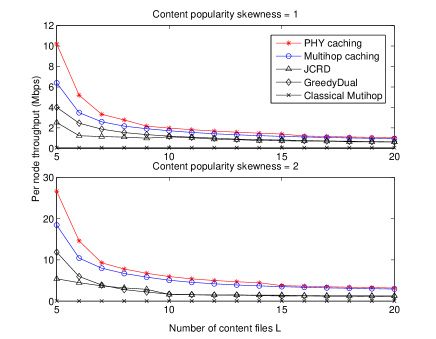
Figure 10: Per node throughput versus the number of content files $L$, where $B_{C}=$4 GB and $\alpha=3.9$.

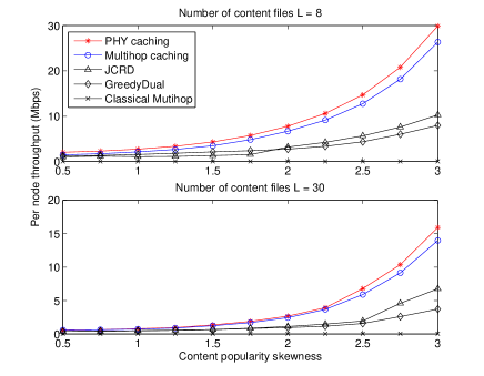
Figure 11: Per node throughput versus the content popularity skewness $\tau$, where $B_{C}=$4 GB and $\alpha=3.9$.

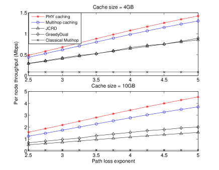
Figure 12: Per node throughput versus the path loss exponent $\alpha$, where $\tau=1$ and $L=20$.

Fig. 10 plots the per node throughput versus the number of files $L$ for $\tau=1$ and $\tau=2$. The multihop caching scheme achieves a much higher throughput than the classical multihop scheme due to the cache-assisted multihopping gain. It also achieves a much higher throughput than the JCRD and GreedyDual schemes due to the MDS encoding gain. Finally, the proposed PHY caching achieves the best performance because it can simultaneously exploit the cache-assisted multihopping gain, the MDS encoding gain and the cache-induced dual-layer CoMP gain.

In Fig. 11, we plot the per node throughput versus the content popularity skewness $\tau$ for $L=8$ and $L=30$ respectively. Again, the proposed PHY caching achieves a significant gain over all baselines. Moreover, even when the cache size at each node is much smaller than the total content size, it is still possible to achieve significant PHY caching gains as $\tau$ becomes large. In practice, the popularity skewness $\tau$ can be large especially for mobile applications [18]. Hence the PHY caching can be a very effective way of enhancing the capacity of wireless networks.

Fig. 12 plots the per node throughput versus the path loss exponent $\alpha$ for $B_{C}=4$ GB and $B_{C}=10$ GB respectively. It can be seen that the three PHY caching gains increase with cache size $B_{C}$.

VII Conclusion

In this paper, we propose a PHY caching scheme to enhance the capacity of wireless adhoc networks. Unlike the existing caching schemes where the cache scheme is usually independent of the PHY, the proposed PHY caching may change the PHY topology (from interference topology to broadcast topology by cache-induced dual-layer CoMP). We establish the corresponding throughput scaling laws under different regimes of file popularity, cache and content size. We further study the impact of various system parameters on the PHY caching gain and provide fundamental design insight for cache-assisted wireless adhoc network. An interesting future work is to establish the information theoretical capacity scaling laws in cache-assisted wireless adhoc networks.

-A Proof of Lemma 1

Proof:

Construct a graph where the vertices are the nodes. There is an edge between any two nodes with distance no more than $r_{I}$. Then finding a frequency reuse scheme which satisfies Condition 1 is a vertex coloring problem. It is known that a graph of degree no more than $D_{G}$ can have its vertices colored by no more than $D_{G}+1$ colors, with no two neighboring vertices having the same color [25]. One can therefore allocate the cells with no more than $D_{G}+1$ subbands such that Condition 1 is satisfied. The rest is to bound $D_{G}$, which is the number of nodes in a circle with radius $r_{I}$ (including the boundary). Using Assumption 1-1), we have $\frac{D_{G}\pi r_{\textrm{min}}^{2}}{4}\leq\pi\left(r_{I}+\frac{r_{\textrm{min}}}{2}\right)^{2}$, which implies that $D_{G}\leq\left(\frac{2r_{I}}{r_{\textrm{min}}}+1\right)^{2}$. ∎

-B Proof of Lemma 2

Proof:

For each link, the bandwidth is $\frac{W}{9}$ and the transmit power on this bandwidth is $P$. The noise power is $\frac{W}{9}$ and it can be shown that the interference power is $PI_{R}$. Hence the SINR of each link is $\frac{9Pr_{0}^{-\alpha}}{W+9PI_{R}}$ and the corresponding rate is $WR_{b}$. Finally, it follows from $\alpha>2$ that $I_{R}=\Theta\left(1\right)$. ∎

-C Proof of Theorem 1

Proof:

Suppose node $n$ requests file $l$. According to the proposed source node set selection scheme, for each requested file segment, $q_{l}L_{S}$ parity bits are obtained from the local cache at node $n$, a total number of $4mq_{l}L_{S}$ parity bits are obtained from the source nodes in $\mathcal{B}_{n,m}$ for $1\leq m<\phi\left(q_{l}\right)$, and a total number of $\left(1-\left(1+2\phi^{2}\left(q_{l}\right)-2\phi\left(q_{l}\right)\right)q_{l}\right)L_{S}$ parity bits are obtained from the source nodes in $\mathcal{B}_{n,\phi\left(q_{l}\right)}$. As a result, the traffic rate $T_{l}$ induced by a single node requesting the $l$-th file is

$$T_{l} = \sum_{m=1}^{\phi\left(q_{l}\right)-1}4m^{2}q_{l}R+\phi\left(q_{l}\right)\left(1-\left(1+2\phi^{2}\left(q_{l}\right)-2\phi\left(q_{l}\right)\right)q_{l}\right)R$$

$$= \left(\phi\left(q_{l}\right)\left(1-q_{l}\right)-\frac{2}{3}(\phi^{3}\left(q_{l}\right)-\phi\left(q_{l}\right))q_{l}\right)R.$$

Note that the ratio between the number of links and the number of nodes is $\lim_{N\rightarrow\infty}\frac{2N-2\sqrt{N}}{N}=2$. Since all links are symmetric, the total traffic rate induced by all nodes are equally partitioned among all links. Hence, the corresponding traffic rate on each link is $\frac{1}{2}\sum_{l=1}^{L}p_{l}T_{l}=\sum_{l=1}^{L}p_{l}\psi\left(q_{l}\right)R$ and we must have $\sum_{l=1}^{L}p_{l}\psi\left(q_{l}\right)R\leq W_{b}R_{b}$, i.e., a per node throughput of $R=\frac{W_{b}R_{b}}{\sum_{l=1}^{L}p_{l}\psi\left(q_{l}\right)}$ is achievable. ∎

-D Proof of Theorem 2

Proof:

Without loss of generality, we focus on the layer 1 CoMP transmission. Consider an achievable scheme where the nodes in $\mathcal{N}_{C}^{1}$ always transmit to all the nodes in $\mathcal{N}_{C}^{2}$ using CoMP transmission (for a node in $\mathcal{N}_{C}^{2}$ without requesting a file with CoMP cache mode, the nodes in $\mathcal{N}_{C}^{1}$ simply transmit dummy packets to this node). At each time slot, the node clusters are randomly formed such that each cluster contains $N_{c}$ adjacent Tx nodes in $\mathcal{N}_{C}^{1}$ and $N_{c}$ adjacent Rx nodes in $\mathcal{N}_{C}^{2}$ that collocated in a square area. Consider the dual network [26] of the original network where the nodes in $\mathcal{N}_{C}^{2}$ act as the transmitters and the nodes in $\mathcal{N}_{C}^{1}$ act as the receivers. We first study the per cluster average sum rate of the dual network. Then the results can be transferred to the original network using the network duality in [26].

Consider the following achievable scheme for the dual network. In each cluster, the nodes in $\mathcal{N}_{C}^{2}$ whose distance from the cluster boundary is less than a threshold $d_{b}=\Theta\left(\left(N_{c}r_{0}\right)^{\frac{1}{2\left(\alpha-1\right)}}\right)$ is not allowed to transmit for interference control. The other $\overline{N}_{c}=\Theta\left(N_{c}-N_{c}^{\frac{\alpha}{2\left(\alpha-1\right)}}\right)$ nodes in $\mathcal{N}_{C}^{2}$ are scheduled to transmit at a constant power $P^{{}^{\prime}}=\frac{9W_{c}P}{W+7W_{c}}=\Theta\left(P\right)$. Let us focus on a reference cluster. Let $\mathcal{G}_{0}^{\textrm{Rx}}$ and $\mathcal{G}_{0}^{\textrm{Tx}}$ denote the set of $N_{c}$ Rx nodes and the set of $\overline{N}_{c}$ scheduled Tx nodes in the reference cluster, respectively. Let $\mathcal{G}_{0}^{\textrm{I}}$ denote the set of scheduled Tx (interfering) nodes from other clusters. By treating the inter-cluster interference as noise, we can achieve the following per cluster average sum rate

$$C_{u}=W_{c}\textrm{E}\left[\log\left|\mathbf{I}+P^{{}^{\prime}}\mathbf{\Omega}^{-1}\mathbf{H}_{c}\mathbf{H}_{c}^{H}\right|\right],$$

where $\mathbf{H}_{c}=\left[h_{i,j}\right]_{\forall i\in\mathcal{G}_{0}^{\textrm{Rx}},j\in\mathcal{G}_{0}^{\textrm{Tx}}}\in\mathbb{C}^{N_{c}\times\overline{N}_{c}}$ is the channel matrix of the reference cluster, $\mathbf{\Omega}=P^{{}^{\prime}}\sum_{n\in\mathcal{G}_{0}^{\textrm{I}}}\mathbf{h}_{I,n}\mathbf{h}_{I,n}^{H}+W_{c}\mathbf{I}$ is the covariance of the inter-cluster interference plus noise at the Rx nodes, and $\mathbf{h}_{I,n}=\left[h_{i,n}\right]_{\forall i\in\mathcal{G}_{0}^{\textrm{Rx}}}\in\mathbb{C}^{N_{c}\times 1}$ is the channel vector from node $n$ to $\mathcal{G}_{0}^{\textrm{Rx}}$. Noting that $\mathbf{h}_{I,n},n\in\mathcal{G}_{0}^{\textrm{I}}$ has independent elements and $\mathbf{h}_{I,n}$ is also independent of $\mathbf{H}_{c}$, we have $\textrm{E}\left[\mathbf{h}_{I,n}\mathbf{h}_{I,n}^{H}|\mathbf{H}_{c}\right]=\textrm{E}\left[\mathbf{h}_{I,n}\mathbf{h}_{I,n}^{H}\right]=\textrm{diag}\left(\left[r_{i,n}^{-\alpha}\right]_{\forall i\in\mathcal{G}_{0}^{\textrm{Rx}}}\right)$. Moreover, using the fact that the nearest interfering node in $\mathcal{N}_{C}^{2}$ is at least $d_{b}$ away from the Rx nodes in $\mathcal{N}_{C}^{1}$, it can be shown that $\sum_{n\in\mathcal{G}_{I}}r_{i,n}^{-\alpha}=O\left(d_{b}^{2-\alpha}\right),\forall i\in\mathcal{G}_{0}^{\textrm{Rx}}$. Hence

$$\textrm{E}\left[\mathbf{\Omega}|\mathbf{H}_{c}\right]=\left(O\left(Pd_{b}^{2-\alpha}\right)+W_{c}\right)\mathbf{I}.$$ (14)

Then we have

$$C_{u} \overset{\textrm{a}}{\geq} W_{c}\textrm{E}\left[\log\left|\mathbf{I}+P^{{}^{\prime}}\textrm{E}\left[\mathbf{\Omega}|\mathbf{H}_{c}\right]^{-1}\mathbf{H}_{c}\mathbf{H}_{c}^{H}\right|\right]$$ (15)

$$\overset{\textrm{b}}{=} W_{c}\textrm{E}\left[\log\left|\mathbf{I}+\frac{P^{{}^{\prime}}}{W_{c}+O\left(Pd_{b}^{2-\alpha}\right)}\mathbf{H}_{c}\mathbf{H}_{c}^{H}\right|\right]$$

$$\overset{\textrm{c}}{=} W_{c}\textrm{E}\left[\log\left|\mathbf{I}+\frac{P^{{}^{\prime}}}{W_{c}}\mathbf{H}_{c}^{H}\mathbf{H}_{c}\right|\right]+O\left(PN_{c}^{\frac{\alpha}{2\left(\alpha-1\right)}}\right),$$

where (15-a) follows from Jensen’s inequality, and (15-b) follows from (14). (15-c) is true because

$$\log\left|\mathbf{I}+\frac{P^{{}^{\prime}}}{W_{c}+O\left(P^{{}^{\prime}}d_{b}^{2-\alpha}\right)}\mathbf{H}_{c}\mathbf{H}_{c}^{H}\right|$$ (16)

$$= \sum_{i=1}^{\overline{N}_{c}}\log\left(1+\frac{P^{{}^{\prime}}}{W_{c}+O\left(P^{{}^{\prime}}d_{b}^{2-\alpha}\right)}\lambda_{i}\right)$$

$$\overset{\textrm{a}}{=} \sum_{i=1}^{\overline{N}_{c}}\log\left(1+\frac{P^{{}^{\prime}}}{W_{c}}\lambda_{i}\right)+O\left(P^{{}^{\prime}}\overline{N}_{c}d_{b}^{2-\alpha}\right)$$

$$\overset{\textrm{b}}{=} \log\left|\mathbf{I}+\frac{P^{{}^{\prime}}\mathbf{H}_{c}^{H}\mathbf{H}_{c}}{W_{c}}\right|+O\left(PN_{c}^{\frac{\alpha}{2\left(\alpha-1\right)}}\right),$$

where $\lambda_{i}$ is the $i$-th eigenvalue of $\mathbf{H}_{c}^{H}\mathbf{H}_{c}$, (16-a) follows from the first order Taylor expansion: $\log\left(1+\frac{P^{{}^{\prime}}}{W_{c}+x}\lambda_{i}\right)=\log\left(1+\frac{P^{{}^{\prime}}}{W_{c}}\lambda_{i}\right)+O\left(x\right)$, (16-b) follows from $\log\left|\mathbf{I}+\frac{P^{{}^{\prime}}\mathbf{H}_{c}^{H}\mathbf{H}_{c}}{W_{c}}\right|=\sum_{i=1}^{\overline{N}_{c}}\log\left(1+\frac{P^{{}^{\prime}}}{W_{c}}\lambda_{i}\right)$, $P^{{}^{\prime}}=\Theta\left(P\right)$, $\overline{N}_{c}=O\left(N_{c}\right)$ and $d_{b}=\Theta\left(N_{c}^{\frac{1}{2\left(\alpha-1\right)}}\right)$.

We can use the same technique as in Appendix I of [19] to bound the term $\overline{C}_{u}\triangleq W_{c}\textrm{E}\left[\log\left|\mathbf{I}+\frac{P^{{}^{\prime}}}{W_{c}}\mathbf{H}_{c}^{H}\mathbf{H}_{c}\right|\right]$. Let $\lambda$ be chosen uniformly among the $\overline{N}_{c}$ eigenvalues of $\frac{\mathbf{H}_{c}^{H}\mathbf{H}_{c}}{\overline{N}_{c}}$. Then

$$\overline{C}_{u} \geq W_{c}\overline{N}_{c}\textrm{E}\left[\log\left(1+\frac{\overline{N}_{c}P^{{}^{\prime}}}{W_{c}}\lambda\right)\right]$$ (17)

$$\geq W_{c}\overline{N}_{c}\log\left(1+\frac{\overline{N}_{c}P^{{}^{\prime}}}{W_{c}}t\right)\Pr\left(\lambda>t\right),$$

for any $t\geq 0$. By the Paley-Zygmund inequality, we have

$$\Pr\left(\lambda>t\right)\geq\frac{\left(\textrm{E}\left(\lambda\right)-t\right)^{2}}{\textrm{E}\left(\lambda^{2}\right)},\>0\leq t<\textrm{E}\left(\lambda\right).$$ (18)

Let $\overline{\mathcal{G}}_{0}^{\textrm{Rx}}$ denote the set of all Rx nodes excluding the Rx nodes in $\mathcal{G}_{0}^{\textrm{Rx}}$. We have

$$\sum_{i\in\overline{\mathcal{G}}_{0}^{\textrm{Rx}}}r_{i,k}^{-\alpha} \underset{\leq}{\textrm{a}} 4r_{0}^{-\alpha}\sum_{j=\left\lceil\frac{d_{b}}{r_{0}}\right\rceil}^{\infty}\sum_{i=-\infty}^{\infty}\left(i^{2}+j^{2}\right)^{-\frac{\alpha}{2}}$$ (19)

$$= \Theta\left(\int_{\left\lceil\frac{d_{b}}{r_{0}}\right\rceil}^{\infty}\int_{-\infty}^{\infty}\left(x^{2}+y^{2}\right)^{-\frac{\alpha}{2}}dxdy\right)$$

$$\overset{\textrm{b}}{=} \Theta\left(\frac{2\sqrt{\pi}\mathbb{G}\left(\frac{\alpha-1}{2}\right)\left\lceil\frac{d_{b}}{r_{0}}\right\rceil^{2-\alpha}}{(\alpha-2)^{2}\mathbb{G}\left(\frac{\alpha}{2}-1\right)}\right)$$

$$= \Theta\left(N_{c}^{-\frac{\alpha-2}{2\left(\alpha-1\right)}}\right)\overset{\textrm{c}}{=}\Theta\left(d_{b}^{2-\alpha}\right),\forall k\in\mathcal{G}_{0}^{\textrm{Tx}},$$

where (19-a) is true because the nearest node in $\overline{\mathcal{G}}_{0}^{\textrm{Rx}}$ is at least $d_{b}$ away from a node in $\mathcal{G}_{0}^{\textrm{Tx}}$, $\mathbb{G}\left(\cdot\right)$ is the Gamma function and (19-b) follows from a direct calculation of the two-dimensional integration, (19-c) follows from $d_{b}=\Theta\left(\left(N_{c}r_{0}\right)^{\frac{1}{2\left(\alpha-1\right)}}\right)$. It follows from (19) that

$$\sum_{i\in\overline{\mathcal{G}}_{0}^{\textrm{Rx}}}r_{i,k}^{-\alpha}=O\left(N_{c}^{-\frac{\alpha-2}{2\left(\alpha-1\right)}}\right),\forall k\in\mathcal{G}_{0}^{\textrm{Tx}}.$$ (20)

Then it follows from (20) and $\sum_{i\in\mathcal{G}_{0}^{\textrm{Rx}}}r_{i,k}^{-\alpha}=G_{C}-\sum_{i\in\overline{\mathcal{G}}_{0}^{\textrm{Rx}}}r_{i,k}^{-\alpha}$ that

$$\sum_{i\in\mathcal{G}_{0}^{\textrm{Rx}}}r_{i,k}^{-\alpha}=G_{C}+O\left(N_{c}^{-\frac{\alpha-2}{2\left(\alpha-1\right)}}\right),\forall k\in\mathcal{G}_{0}^{\textrm{Tx}},$$ (21)

where $G_{C}\triangleq\sum_{i\in\mathcal{G}_{0}^{\textrm{Rx}}\cup\overline{\mathcal{G}}_{0}^{\textrm{Rx}}}r_{i,k}^{-\alpha}$ is defined in Theorem 2. Following similar analysis as in Appendix I of [19], we have

$$\textrm{E}\left(\lambda\right) = \frac{1}{\overline{N}_{c}}\textrm{E}\left(\textrm{Tr}\left(\frac{\mathbf{H}_{c}^{H}\mathbf{H}_{c}}{\overline{N}_{c}}\right)\right)$$ (22)

$$= \frac{1}{\overline{N}_{c}^{2}}\sum_{k\in\mathcal{G}_{0}^{\textrm{Tx}}}\sum_{i\in\mathcal{G}_{0}^{\textrm{Rx}}}\textrm{E}\left(\left|h_{i,k}\right|^{2}\right)$$

$$= \frac{1}{\overline{N}_{c}^{2}}\sum_{k\in\mathcal{G}_{0}^{\textrm{Tx}}}\sum_{i\in\mathcal{G}_{0}^{\textrm{Rx}}}r_{i,k}^{-\alpha}$$

$$= \frac{G_{C}+O\left(N_{c}^{-\frac{\alpha-2}{2\left(\alpha-1\right)}}\right)}{\overline{N}_{c}},$$

$$\textrm{E}\left(\lambda^{2}\right) = \frac{1}{\overline{N}_{c}}\textrm{E}\left(\textrm{Tr}\left(\frac{\mathbf{H}_{c}^{H}\mathbf{H}_{c}\mathbf{H}_{c}^{H}\mathbf{H}_{c}}{\overline{N}_{c}^{2}}\right)\right)$$ (23)

$$= \frac{1}{\overline{N}_{c}^{3}}\sum_{k\in\mathcal{G}_{0}^{\textrm{Tx}}}\sum_{i\in\mathcal{G}_{0}^{\textrm{Rx}}}\sum_{m\in\mathcal{G}_{0}^{\textrm{Tx}}}\sum_{l\in\mathcal{G}_{0}^{\textrm{Rx}}}\textrm{E}\left(h_{i,k}h_{l,k}^{*}h_{l,m}h_{i,m}^{*}\right)$$

$$\leq \frac{2}{\overline{N}_{c}^{3}}\sum_{k\in\mathcal{G}_{0}^{\textrm{Tx}}}\sum_{i\in\mathcal{G}_{0}^{\textrm{Rx}}}\sum_{l\in\mathcal{G}_{0}^{\textrm{Rx}}}\textrm{E}\left(\left|h_{i,k}\right|^{2}\right)\textrm{E}\left(\left|h_{l,k}\right|^{2}\right)$$

$$= \frac{2}{\overline{N}_{c}^{3}}\sum_{k\in\mathcal{G}_{0}^{\textrm{Tx}}}\sum_{i\in\mathcal{G}_{0}^{\textrm{Rx}}}r_{i,k}^{-\alpha}\sum_{l\in\mathcal{G}_{0}^{\textrm{Rx}}}r_{l,k}^{-\alpha}$$

$$= \frac{2\left(G_{C}+O\left(N_{c}^{-\frac{\alpha-2}{2\left(\alpha-1\right)}}\right)\right)^{2}}{\overline{N}_{c}^{2}}.$$

where the last equalities in the above two equations follow from (21) and $\sum_{k\in\mathcal{G}_{0}^{\textrm{Tx}}}=\overline{N}_{c}$. Choosing $t=\frac{r_{0}^{-\alpha}}{\overline{N}_{c}}$ and using (17), (18), (22) and (23), we have

$$\overline{C}_{u}\geq W_{c}\overline{N}_{c}\rho\log\left(1+\frac{P^{{}^{\prime}}r_{0}^{-\alpha}}{W_{c}}\right)+O\left(PN_{c}^{\frac{\alpha}{2\left(\alpha-1\right)}}\right).$$

According to the network duality in [26], a per cluster average sum rate of $C_{d}=C_{u}\geq\overline{C}_{u}+O\left(PN_{c}^{\frac{\alpha}{2\left(\alpha-1\right)}}\right)$ can be achieved in the original network with equal or less total network power. Since the clusters are randomly formed, all nodes in $\mathcal{N}_{C}^{1}$ (or in $\mathcal{N}_{C}^{2}$) are statistically symmetric. As a result, the per node average rate $R_{c}^{{}^{\prime}}$ that can be provided by the PHY is lower bounded as

$$R_{c}^{{}^{\prime}} \geq \frac{C_{d}}{N_{c}}\geq\rho W_{c}\log\left(1+\frac{P^{{}^{\prime}}r_{0}^{-\alpha}}{W_{c}}\right)+O\left(PN_{c}^{-\frac{\alpha-2}{2\left(\alpha-1\right)}}\right)$$ (24)

$$\overset{\textrm{a}}{\geq} \rho W_{c}\log\left(1+\frac{2Pr_{0}^{-\alpha}}{W}\right)+O\left(PN_{c}^{-\frac{\alpha-2}{2\left(\alpha-1\right)}}\right)$$

and the average power at each node in $\mathcal{N}_{C}^{1}$ required to achieve the above per node average rate is no more than $P^{{}^{\prime}}$, where (24-a) follows from $\frac{P^{{}^{\prime}}}{W_{c}}=\frac{9P}{W+7W_{c}}\geq\frac{2P}{W}$. On the other hand, using the cut set bound between all nodes in $\mathcal{N}_{C}^{1}$ and a node in $\mathcal{N}_{C}^{2}$, we have

$$R_{c}^{{}^{\prime}}\leq W_{c}\log\left(1+\frac{P^{{}^{\prime}}G_{C}}{W_{c}}\right)\overset{\textrm{a}}{\leq}W_{c}\log\left(1+\frac{9PG_{C}}{W}\right),$$ (25)

where (25-a) follows from $\frac{P^{{}^{\prime}}}{W_{c}}=\frac{9P}{W+7W_{c}}\leq\frac{9P}{W}$. ∎

-E Proof of Corollary 1

Proof:

Let us first consider the case when $Q_{\Omega\left(\mathbf{q}\right)}>0$ and $Q_{\overline{\Omega}\left(\mathbf{q}\right)}>0$. Consider the transmission of $L_{0}$ files to a reference node $n_{0}$. Following similar analysis as that in Appendix -C, it can be shown that the per link multihop traffic (i.e., the traffic of each link on the multihop band) induced by transmitting files with multihop cache mode is $\sum_{l\in\Omega\left(\mathbf{q}\right)}FL_{l}\psi\left(q_{l}\right)$, where $L_{l}$ is the number of transmitting the $l$-th file. Clearly, the CoMP traffic (i.e., the traffic delivered to node $n_{0}$ on CoMP band) induced by transmitting files with CoMP cache mode is $\sum_{l\in\overline{\Omega}\left(\mathbf{q}\right)}FL_{l}\left(1-q_{l}\right)$. The transmission of $L_{0}$ files can be finished within time $t_{0}$ if and only if both the per link multihop traffic can be delivered on the multihop band and the CoMP traffic can be delivered on the CoMP band, i.e., $\sum_{l\in\Omega\left(\mathbf{q}\right)}FL_{l}\psi\left(q_{l}\right)\leq\left(W-2W_{c}\right)R_{m}\left(W_{c}\right)t_{0}$ and $\sum_{l\in\overline{\Omega}\left(\mathbf{q}\right)}FL_{l}\left(1-q_{l}\right)\leq W_{c}R_{c}\left(W_{c}\right)t_{0}$. Hence, the per node throughput for fixed bandwidth partition $W_{c},W_{b}=W-2W_{c}$ is

$$T_{\mathbf{q}}\left(W_{c}\right)$$

$$= \lim_{L_{0}\rightarrow\infty}\frac{L_{0}F}{t_{0}}$$

$$= \lim_{L_{0}\rightarrow\infty}\frac{L_{0}F}{\max\left(\frac{\sum_{l\in\Omega\left(\mathbf{q}\right)}FL_{l}\psi\left(q_{l}\right)}{\left(W-2W_{c}\right)R_{m}\left(W_{c}\right)},\frac{\sum_{l\in\overline{\Omega}\left(\mathbf{q}\right)}FL_{l}\left(1-q_{l}\right)}{W_{c}R_{c}\left(W_{c}\right)}\right)}$$

$$= \lim_{L_{0}\rightarrow\infty}\frac{1}{\max\left(\frac{Q_{\Omega\left(\mathbf{q}\right)}}{\left(W-2W_{c}\right)R_{m}\left(W_{c}\right)},\frac{Q_{\overline{\Omega}\left(\mathbf{q}\right)}}{W_{c}R_{c}\left(W_{c}\right)}\right)},$$

where the last equality follows from $\lim_{L_{0}\rightarrow\infty}\frac{L_{l}}{L_{0}}=p_{l}$. Hence, the per node throughput $\Gamma_{A}\left(\mathbf{q}\right)=\max_{W_{c}\in\left(0,W_{c}\right)}T_{\mathbf{q}}\left(W_{c}\right)=T_{\mathbf{q}}\left(W_{c}^{*}\right)$, where the optimal solution $W_{c}^{*}$ is the unique solution of (5). Using (5), it can be verified that $T_{\mathbf{q}}\left(W_{c}^{*}\right)$ is given by (4).

It can be verified that $\Gamma_{A}\left(\mathbf{q}\right)$ is still given by (6) when $Q_{\Omega\left(\mathbf{q}\right)}=0$ or $Q_{\overline{\Omega}\left(\mathbf{q}\right)}=0$. Moreover, $\Gamma_{A}^{U}\left(\mathbf{q}\right)\geq\Gamma_{A}\left(\mathbf{q}\right)\geq\Gamma_{A}^{L}\left(\mathbf{q}\right)+O\left(PN_{c}^{-\frac{\alpha-2}{2\left(\alpha-1\right)}}\right)$ follows from that $\Gamma_{A}\left(\mathbf{q}\right)$ is an increasing function of $R_{m}\left(W_{c}^{*}\right)$ and $R_{c}\left(W_{c}^{*}\right)$. Finally, as $P,N_{c}\rightarrow\infty$ such that $PN_{c}^{-\frac{\alpha-2}{2\left(\alpha-1\right)}}\rightarrow 0$, we have $R_{m}^{a}\rightarrow\frac{1}{9}\log\left(1+\frac{r_{0}^{-\alpha}}{I_{R}}\right)$ and $R_{m}^{a}/R_{c}^{a}\rightarrow 0,$ for $a\in\left\{L,U\right\}$, from which (7) follows. ∎

-F Proof of Corollary 2

Proof:

When $q_{l}=o\left(1\right)$, it can be shown that $\psi\left(q_{l}\right)=\Theta\left(\sqrt{\frac{1}{q_{l}}}\right)$. When $q_{l}=\Theta\left(1\right)$, it can be shown that $\psi\left(q_{l}\right)=O\left(1\right)$. Let $\mathcal{L}_{1}=\left\{l:\>q_{l}=\Theta\left(1\right)\right\}$. Since $\sum_{l=1}^{L}q_{l}\leq\frac{B_{C}}{F}$, the cardinality of $\mathcal{L}_{1}$ must be bounded, i.e., $\left|\mathcal{L}_{1}\right|=\Theta\left(1\right)$. As a result, we have $\sum_{l\in\mathcal{L}_{1}}p_{l}\psi\left(q_{l}\right)=O\left(1\right)$ and

$$\sum_{l=1}^{L}p_{l}\psi\left(q_{l}\right)$$ (26)

$$= \Theta\left(\sum_{l\notin\mathcal{L}_{1}}p_{l}\sqrt{\frac{1}{q_{l}}}\right)+\sum_{l\in\mathcal{L}_{1}}p_{l}\psi\left(q_{l}\right)$$

$$= \Theta\left(\sum_{l}p_{l}\sqrt{\frac{1}{q_{l}}}\right)-\Theta\left(\sum_{l\in\mathcal{L}_{1}}p_{l}\sqrt{\frac{1}{q_{l}}}\right)+O\left(1\right)$$

$$= \Theta\left(\sum_{l}p_{l}\sqrt{\frac{1}{q_{l}}}\right)+O\left(1\right)=\Theta\left(\sum_{l}p_{l}\sqrt{\frac{1}{q_{l}}}\right),$$

where the last equality holds because $\Theta\left(\sum_{l}p_{l}\sqrt{\frac{1}{q_{l}}}\right)\geq\Theta\left(1\right)$. It follows from (26) and Theorem 1 that $\Gamma_{B}\left(\mathbf{q}\right)=\Theta\left(\frac{1}{\sum_{l=1}^{L}p_{l}\sqrt{\frac{1}{q_{l}}}}\right)$. For bounded power $P$ and $\alpha>2$, it can be shown that the interference seen at any node is bounded, from which it follows that $R_{c}\left(W_{c}\right)=\Theta\left(1\right)$. Hence, $\Gamma_{A}\left(\mathbf{q}\right)=\Theta\left(\frac{1}{Q_{\Omega\left(\mathbf{q}\right)}+2Q_{\overline{\Omega}\left(\mathbf{q}\right)}}\right)=\Theta\left(\sum_{l}p_{l}\sqrt{\frac{1}{q_{l}}}\right)$, where the last equality follows similar analysis as in (26). ∎

-G Proof of Theorem 3

Proof:

Consider the following relaxed problem:

$$\min_{\mathbf{q}>0}\>f\left(\mathbf{q}\right)\triangleq\sum_{l=1}^{L}p_{l}\sqrt{\frac{1}{q_{l}}},\>s.t.\>\sum_{l=1}^{L}q_{l}\leq\frac{B_{C}}{F}.$$ (27)

Using the Lagrange dual method, it can be shown that the optimal solution and the optimal value of Problem (27) are given by $q_{l}^{\star}=\frac{B_{C}p_{l}^{2/3}}{F\sum_{l=1}^{L}p_{l}^{2/3}},\forall l$ and $f\left(\mathbf{q}^{\star}\right)=\sqrt{\frac{F}{B_{C}}}\left[\sum_{l=1}^{L}p_{l}^{2/3}\right]^{3/2}$, respectively. On the other hand, the objective value of Problem (8) with cache content replication vector $\mathbf{q}^{*}$ in (9) is given by $f\left(\mathbf{q}^{*}\right)\leq f\left(\mathbf{q}^{*}-\frac{1}{N}\right)=\Theta\left(\left[\sum_{l=1}^{L}p_{l}^{2/3}\right]^{3/2}\right)$. Let $f^{*}$ denote the optimal value of Problem (8). Since $f\left(\mathbf{q}^{\star}\right)\leq f^{*}\leq f\left(\mathbf{q}^{*}\right)$, $f\left(\mathbf{q}^{\star}\right)=\Theta\left(\left[\sum_{l=1}^{L}p_{l}^{2/3}\right]^{3/2}\right)$ and $f\left(\mathbf{q}^{*}\right)\leq\Theta\left(\left[\sum_{l=1}^{L}p_{l}^{2/3}\right]^{3/2}\right)$, we have $f^{*}=\Theta\left(\left[\sum_{l=1}^{L}p_{l}^{2/3}\right]^{3/2}\right)$, which proves that $\mathbf{q}^{*}$ is the order-optimal cache content replication vector. ∎

-H Proof of Theorem 4

Consider a simple bandwidth partition: $W_{b}=W_{c}=\frac{W}{3}$. We first prove that a throughput of $\Theta\left(\frac{C_{B}}{\sum_{l=1}^{L}p_{l}\sqrt{\frac{1}{q_{l}}}}\right)$, where $C_{B}\triangleq\frac{W}{M}\log\left(1+\frac{3MP\left(2r_{\textrm{max}}\right)^{-\alpha}}{\left(M+1\right)W+3MI_{A}}\right)$, is achievable for node $n$ requesting a file $l_{n}$ with multihop cache mode. The proof relies on Lemma 1 and the following lemma.

Lemma 3 (Upper bound of source radius).

For a node $n$ requesting a file $l_{n}$ with multihop cache mode

$$r_{n}^{*}\leq\left(2\sqrt{\left\lceil 1/q_{l_{n}}\right\rceil-1}+1\right)r_{\textrm{max}}.$$

Proof:

Let $\mathcal{O}_{n}$ denote a disk centered at the node $n$ with radius $r_{n}^{*}-r_{\textrm{max}}$ and let $\mathcal{O}_{n}^{{}^{\prime}}$ denote the intersection of $\mathcal{O}_{n}$ and the network coverage area (i.e., the square of area $Nr_{0}^{2}$). By Assumption 1-2), any point inside $\mathcal{O}_{n}^{{}^{\prime}}$ must lie in the Voronoi cells corresponding to the nodes in $\overline{\mathcal{B}}_{n}\cup n$. Since the area of each Voronoi cell is less than $\pi r_{\textrm{max}}^{2}$, we must have $\mathcal{A}\left(\mathcal{O}_{n}^{{}^{\prime}}\right)\leq\left(\left|\overline{\mathcal{B}}_{n}\right|+1\right)\pi r_{\textrm{max}}^{2}$, where $\mathcal{A}\left(\mathcal{O}_{n}^{{}^{\prime}}\right)$ denotes the area of $\mathcal{O}_{n}^{{}^{\prime}}$. Since $\mathcal{A}\left(\mathcal{O}_{n}^{{}^{\prime}}\right)\geq\frac{\pi\left(r_{n}^{*}-r_{\textrm{max}}\right)^{2}}{4}$ and $\left|\overline{\mathcal{B}}_{n}\right|\leq\left\lceil 1/q\right\rceil-2$, we have $\frac{\pi\left(r_{n}^{*}-r_{\textrm{max}}\right)^{2}}{4}\leq\left(\left\lceil 1/q\right\rceil-1\right)\pi r_{\textrm{max}}^{2}$ and thus $r_{n}^{*}\leq\left(2\sqrt{\left\lceil 1/q\right\rceil-1}+1\right)r_{\textrm{max}}$. ∎

We first derive a lower bound for the throughput of each link on the multihop band. For each link, the bandwidth is $\frac{W}{3M}$ and the transmit power on this bandwidth is $\frac{P}{1+M}$. The noise power is $\frac{W}{3M}$ and the interference power is upper bounded by $\frac{P}{1+M}I_{A}$ as will be shown later. The channel gain of each link is lower bounded by $\left(2r_{\textrm{max}}\right)^{-\alpha}$ since the distance between any two adjacent nodes is upper bounded by $2r_{\textrm{max}}$ by Assumption 1-2). It follows that the throughput of each link is lower bounded by $\frac{C_{B}}{3}$.

Suppose we want to support a per node throughput of $R$. Using Assumption 1 and Lemma 3, it can be shown that the average traffic $T_{n}$ to be relayed by the $n$-th node on the multihop band is upper bounded as $T_{n}\leq\Theta\left(\sum_{l=1}^{L}p_{l}\sqrt{\frac{1}{q_{l}}}R\right)$ for all $n$. Clearly, a per node throughput of $R$ can be supported if no node is overloaded, i.e., $T_{n}\leq\frac{C_{B}}{3},\forall n$. Hence, a per node throughput of $R=\Theta\left(\frac{C_{B}}{\sum_{l=1}^{L}p_{l}\sqrt{\frac{1}{q_{l}}}}\right)$ is achievable.

The rest is to prove that the interference power $I_{B}$ seen at each node on the multihop band is upper bounded by $\frac{1}{3M}I_{A}$. For any node $n$, let $\mathcal{O}_{n}\left(ix\right)$ denote a disk centered at the node $n$ with radius $ix$ and define a set of rings $\mathcal{O}_{n,i}\triangleq\mathcal{O}_{n}\left(\left(i+1\right)x\right)\backslash\mathcal{O}_{n}\left(ix\right),i=1,2,...$. Using Assumption 1-1), it can be shown that the number of nodes in the $i$-th ring $\mathcal{O}_{n,i}$ is upper bounded by $\frac{\left(\left(i+1\right)x+\frac{r_{\textrm{min}}}{2}\right)^{2}-\left(ix-\frac{r_{\textrm{min}}}{2}\right)^{2}}{r_{\textrm{min}}^{2}/4}$. Clearly, the distance between a node in $\mathcal{O}_{n,i}$ and node $n$ is lower bounded by $ix$. Moreover, from Assumption 1-2) and Condition 1, there is no interference from the nodes in $\mathcal{O}_{n}\left(r_{I}-2r_{\textrm{max}}\right)$ to node $n$. As a result, if we let $x=r_{I}-2r_{\textrm{max}}$, the interference power $I_{B}$ seen by any node can be upper bounded as

$$I_{B} \leq \sum_{i=1}^{\infty}\frac{\left(\left(i+1\right)x+\frac{r_{\textrm{min}}}{2}\right)^{2}-\left(ix-\frac{r_{\textrm{min}}}{2}\right)^{2}}{r_{\textrm{min}}^{2}/4}\frac{P}{\left(1+M\right)\left(ix\right)^{\alpha}}$$

$$\leq \frac{4P\left(x+r_{\textrm{min}}\right)}{\left(1+M\right)r_{\textrm{min}}^{2}}\sum_{i=1}^{\infty}\left(\frac{2}{\left(ix\right)^{\alpha-1}}+\frac{1}{i^{\alpha}x^{\alpha-1}}\right)$$

$$\leq \frac{4P\left(x+r_{\textrm{min}}\right)}{\left(1+M\right)r_{\textrm{min}}^{2}}\left[\int_{1}^{\infty}\left(\frac{2}{\left(zx\right)^{\alpha-1}}+\frac{1}{z^{\alpha}x^{\alpha-1}}\right)dz+\frac{3}{x^{\alpha-1}}\right]$$

$$= \frac{4P\left(x+r_{\textrm{min}}\right)}{\left(1+M\right)r_{\textrm{min}}^{2}x^{\alpha-1}}\left(\frac{2}{\alpha-2}+\frac{1}{\alpha-1}+3\right).$$

On the other hand, when node $n$ requests a file $l_{n}$ with CoMP cache mode, it is clear that a throughput of $\Theta\left(1\right)\geq\Theta\left(\frac{C_{B}}{\sum_{l=1}^{L}p_{l}\sqrt{\frac{1}{q_{l}}}}\right)$ is achievable for node $n$. As a result, an overall throughput of $R=\Theta\left(\frac{C_{B}}{\sum_{l=1}^{L}p_{l}\sqrt{\frac{1}{q_{l}}}}\right)$ is also achievable for node $n$.

References

- [1] S. Goebbels, “Disruption tolerant networking by smart caching,” Int. J. Commun. Syst., vol. 23, no. 5, pp. 569–595, May 2010.
- [2] N. Golrezaei, K. Shanmugam, A. Dimakis, A. Molisch, and G. Caire, “Femtocaching: Wireless video content delivery through distributed caching helpers,” Proc. IEEE INFOCOM, pp. 1107–1115, 2012.
- [3] U. Kozat, O. Harmanci, S. Kanumuri, M. Demircin, and M. Civanlar, “Peer assisted video streaming with supply-demand-based cache optimization,” IEEE Transactions on Multimedia, vol. 11, no. 3, pp. 494–508, 2009.
- [4] B. Shen, S.-J. Lee, and S. Basu, “Caching strategies in transcoding-enabled proxy systems for streaming media distribution networks,” IEEE Transactions on Multimedia, vol. 6, no. 2, pp. 375–386, 2004.
- [5] X. Ge, K. Huang, C.-X. Wang, X. Hong, and X. Yang, “Capacity analysis of a multi-cell multi-antenna cooperative cellular network with co-channel interference,” IEEE Trans. Wireless Commun., vol. 10, no. 10, pp. 3298–3309, October 2011.
- [6] M. Maddah-Ali and U. Niesen, “Fundamental limits of caching,” IEEE Trans. Info. Theory, vol. 60, no. 5, pp. 2856–2867, May 2014.
- [7] E. Bastug, M. Bennis, and M. Debbah, “Living on the edge: The role of proactive caching in 5G wireless networks,” IEEE Communications Magazine, vol. 52, no. 8, pp. 82–89, Aug 2014.
- [8] S. Gitzenis, G. Paschos, and L. Tassiulas, “Asymptotic laws for joint content replication and delivery in wireless networks,” IEEE Trans. Info. Theory, vol. 59, no. 5, pp. 2760–2776, May 2013.
- [9] M. Ji, G. Caire, and A. Molisch, “Fundamental limits of distributed caching in D2D wireless networks,” 2013. [Online]. Available: http://arxiv.org/abs/1304.5856
- [10] M. Ji, G. Caire, and A. F. Molisch, “The throughput-outage tradeoff of wireless one-hop caching networks,” 2013. [Online]. Available: http://arxiv.org/abs/1312.2637
- [11] ——, “Wireless device-to-device caching networks: Basic principles and system performance,” 2013. [Online]. Available: http://arxiv.org/abs/1305.5216
- [12] A. Altieri, P. Piantanida, L. R. Vega, and C. Galarza, “On fundamental trade-offs of device-to-device communications in large wireless networks,” 2014. [Online]. Available: http://arxiv.org/abs/1405.2295
- [13] S.-W. Jeon, S.-N. Hong, M. Ji, and G. Caire, “Caching in wireless multihop device-to-device networks,” in to appear in IEEE ICC 2015, Jun 2015.
- [14] P. Gupta and P. Kumar, “The capacity of wireless networks,” IEEE Trans. Info. Theory, vol. 46, no. 2, pp. 388–404, Mar 2000.
- [15] A. Liu and V. Lau, “Cache-enabled opportunistic cooperative MIMO for video streaming in wireless systems,” IEEE Trans. Signal Processing, vol. 62, no. 2, pp. 390–402, Jan 2014.
- [16] ——, “Mixed-timescale precoding and cache control in cached MIMO interference network,” IEEE Trans. Signal Processing, vol. 61, no. 24, pp. 6320–6332, Dec 2013.
- [17] L. Breslau, P. Cao, L. Fan, G. Phillips, and S. Shenker, “Web caching and zipf-like distributions: evidence and implications,” in Proc. INFOCOM, New York, USA, Mar 1999, pp. 126–134.
- [18] T. Yamakami, “A zipf-like distribution of popularity and hits in the mobile web pages with short life time,” in Proc. Parallel Distrib. Comput., Appl. Technol., Taipei, Taiwan, Dec 2006, pp. 240–243.
- [19] A. Ozgur, O. Leveque, and D. Tse, “Hierarchical cooperation achieves optimal capacity scaling in ad hoc networks,” IEEE Trans. Info. Theory, vol. 53, no. 10, pp. 3549–3572, Oct 2007.
- [20] U. Niesen, P. Gupta, and D. Shah, “The balanced unicast and multicast capacity regions of large wireless networks,” IEEE Trans. Info. Theory, vol. 56, no. 5, pp. 2249–2271, May 2010.
- [21] L. Iacobelli, F. Scoubart, D. Pirez, P. Fouillot, R. Massin, C. Lefebvre, C. Le Martret, and V. Conan, “Dynamic frequency allocation in ad hoc networks,” in 2010 2nd International Workshop on Cognitive Information Processing (CIP), June 2010, pp. 145–150.
- [22] J. Elsner, R. Tanbourgi, and F. Jondral, “On the transmission capacity of wireless multi-channel ad hoc networks with local FDMA scheduling,” in 2010 International Congress on Ultra Modern Telecommunications and Control Systems and Workshops (ICUMT), Oct 2010, pp. 315–320.
- [23] H. Weingarten, Y. Steinberg, and S. Shamai, “The capacity region of the gaussian multiple-input multiple-output broadcast channel,” IEEE Trans. Info. Theory, vol. 52, no. 9, pp. 3936–3964, 2006.
- [24] S. Jin and L.Wang, “Content and service replication strategies in multihop wireless mesh networks,” in in Proc. 8th ACM Int. Symp. Model., Anal. Simul. Wireless Mobile Syst., Montreal, QC, Canada, Oct. 2005, pp. 79–86.
- [25] J. A. Bondy and U. Murthy, Graph Theory with Applications. New York: Elsevier, 1976.
- [26] A. Liu, Y. Liu, H. Xiang, and W. Luo, “MIMO B-MAC interference network optimization under rate constraints by polite water-filling and duality,” IEEE Trans. Signal Processing, vol. 59, no. 1, pp. 263 –276, Jan. 2011.