The exact Taylor formula of the implied volatility

Abstract

In a model driven by a multi-dimensional local diffusion, we study the behavior of implied volatility ${\sigma}$ and its derivatives with respect to log-strike $k$ and maturity $T$ near expiry and at the money. We recover explicit limits of the derivatives ${\partial_{T}^{q}}\partial_{k}^{m}\sigma$ for $(T,x-k)$ approaching the origin within the parabolic region $|x-k|\leq\lambda\sqrt{T}$, with $x$ denoting the spot log-price of the underlying asset and where $\lambda$ is a positive and arbitrarily large constant. Such limits yield the exact Taylor formula for implied volatility within the parabola $|x-k|\leq\lambda\sqrt{T}$. In order to include important models of interest in mathematical finance, e.g. Heston, CEV, SABR, the analysis is carried out under the weak assumption that the infinitesimal generator of the diffusion is only locally elliptic.

Keywords: implied volatility, local-stochastic volatility, local diffusions, Feller process

MSC 2010 numbers: 60J60, 60J70, 91G20

JEL classification codes: C02, C60

1 Introduction

This paper deviates from the mainstream literature on asymptotic methods in finance; in fact, our main result does not add another formula to the plethora of approximation formulas for the implied volatility (IV) already available in the literature. Rather, we prove an exact result: a rigorous derivation of the exact Taylor formula of IV, as a function of both strike and maturity, in a parabolic region close to expiry and at-the-money (ATM).

This is done under general assumptions that allow to include popular models, such as the CEV and the Heston models, as very particular cases: indeed, we consider a multivariate model driven by a stochastic process that is a local diffusion in a sense that suitably generalizes the classical notion of diffusion as given by Stroock and Varadhan (1979) and Friedman (1975, 1976).

The literature on IV asymptotics is extensive and exploits a diverse range of mathematical techniques. Focusing on short-time asymptotics, well-known results were obtained by Berestycki et al. (2002), Berestycki et al. (2004) and Durrleman (2010). Deferring precise definitions until the body of this paper, we denote by ${\sigma}(t,x;T,k)$ the IV related to a Call option with log-strike $k$ and maturity $T$, where $x$ is the spot log-price of the underlying asset at time $t$. Berestycki et al. (2004) uses PDEs techniques to prove the existence of the limits $\lim\limits_{T\rightarrow t^{+}}{\sigma}(t,x;T,k)$ in a generic stochastic volatility model and to characterize such limits in terms of Varadhan’s geodesic distance (see also to Gavalas and Yortsos (1980) for related results). More recently, Durrleman (2010) gives conditions under which it is possible to recover the ATM-limits $\lim\limits_{T\rightarrow t^{+}}{\partial_{T}^{q}}\partial_{k}^{m}\sigma(t,k;T,k)$ using a semi-martingale decomposition of implied volatilities; although this approach performs also in non-Markovian settings, the validity of the conditions for the existence of the limits is verified only under Markovian assumptions and employing the results in Berestycki et al. (2004).

While it is common practice to consider the IV as a function of maturity and strike $(T,k)$, the aforementioned papers examine only the vertical limits, as $T\rightarrow t^{+}$, of $\sigma(t,x;T,k)$. The aim of this paper is to give conditions for the existence and an explicit representation of the limits of ${\partial_{T}^{q}}\partial_{k}^{m}\sigma(t,x;T,k)$, at any order $m,{q}$, as $(T-t,x-k)$ approaches the origin within the parabolic region $\mathcal{P}_{\lambda}:=\{|x-k|\leq\lambda\sqrt{T-t}\}$; here $\lambda$ is an arbitrarily large positive parameter. From a practical perspective, $\mathcal{P}_{\lambda}$ is the region of interest where implied volatility data are typically observed in the market. As a by-product, we also provide a rigorous and explicit derivation of the exact Taylor formula (see formula (1.3) below) for the implied volatility $\sigma(t,x;\cdot,\cdot)$ in $\mathcal{P}_{\lambda}$, around $(T,k)=(t,x)$.

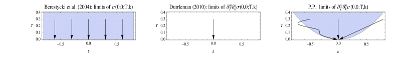
Figure 1: Directions along which the limits are computed in Berestycki et al. (2004), in Durrleman (2010) and in this paper, respectively.

The starting point is the analysis of the transition density first developed in a scalar setting in Pagliarani and Pascucci (2012) and later extended to asymptotic IV expansions in multiple dimensions in Lorig et al. (2015b), where the authors derived a fully explicit approximation, hereafter denoted by $\bar{\sigma}_{N}$, for the IV at any given order $N\in{\mathbb{N}}$. Our main result, Theorem 5.1 below, gives a sharp error bound on ${\partial_{T}^{q}}\partial_{k}^{m}(\sigma-\bar{\sigma}_{N})$ and leads to the existence of the limits

$$\lim_{(T,k)\to(t,x)\atop|x-k|\leq\lambda\sqrt{T-t}}{\partial_{T}^{q}}\partial_{k}^{m}\big{(}\sigma-\bar{\sigma}_{N}\big{)}(t,x;T,k)=0,\qquad 2{q}+m\leq N.$$ (1.1)

In the one-dimensional case and for derivatives of order less than or equal to two, similar results were proved in Bompis and Gobet (2012) by using Malliavin calculus techniques. Our results are proved under mild conditions on the driving stochastic process, which is assumed to be a Feller process and an inhomogeneous local diffusion. Loosely speaking, we assume that the infinitesimal generator of the diffusion is only locally elliptic (i.e. elliptic on a certain domain $D\subseteq{\mathbb{R}}^{d}$) and its coefficients satisfy suitable regularity conditions; note that no ellipticity condition is imposed on the complementary set ${\mathbb{R}}^{d}\setminus D$. Results under such general hypotheses appear to be novel compared to the existing literature. In particular, our analysis includes processes with killing and/or degenerate processes: our assumptions do not even imply that the law of the underlying process has a density and therefore our results apply to many degenerate cases of interest, such as the well-known CEV, Heston and SABR models, among others.

Formula (1.1) implies that the limits of the derivatives ${\partial_{T}^{q}}\partial_{k}^{m}\sigma$ exist if and only if the limits of ${\partial_{T}^{q}}\partial_{k}^{m}\bar{\sigma}_{N}$ do exist, and in that case we have

$$\lim_{(T,k)\to(t,x)\atop|x-k|\leq\lambda\sqrt{T-t}}{\partial_{T}^{q}}\partial_{k}^{m}\sigma(t,x;T,k)=\lim_{(T,k)\to(t,x)\atop|x-k|\leq\lambda\sqrt{T-t}}{\partial_{T}^{q}}\partial_{k}^{m}\bar{\sigma}_{N}(t,x;T,k).$$ (1.2)

Note that, in general, the limits in (1.2) do not exist: a simple example is given in Roper and Rutkowski (2009), Section 6, who exhibit a log-normal model with oscillating time-dependent volatility. In that case the results by Berestycki et al. (2002), Berestycki et al. (2004) and Durrleman (2010) do not apply, while the approximation $\bar{\sigma}_{N}$ in Lorig et al. (2015a) turns out to be exact at order $N=0$. More generally, we shall provide simple and explicit conditions ensuring the existence of the limits of ${\partial_{T}^{q}}\partial_{k}^{m}\bar{\sigma}_{N}$, and consequently the existence of those of ${\partial_{T}^{q}}\partial_{k}^{m}{\sigma}$ in (1.2). A particular case is when the underlying diffusion is time-homogeneous: in that case, $\bar{\sigma}_{N}$ is polynomial in time and thus smooth up to $T=t$.

Denoting by ${\partial_{T}^{q}}\partial_{k}^{m}\bar{\sigma}_{N}(t,x)$ the limits in (1.2), whose explicit expression is known at any order, we get the following exact parabolic Taylor formula for ${\sigma}$:

$${\sigma}(t,x;T,k)=\sum_{2{q}+m\leq N}\frac{{\partial_{T}^{q}}\partial_{k}^{m}{\bar{\sigma}_{N}(t,x)}}{{q}!m!}(T-t)^{q}(k-x)^{m}+\text{\rm o}\left((T-t)^{\frac{N}{2}}+|k-x|^{N}\right),$$ (1.3)

as $(T,k)\to(t,x)$ in $\mathcal{P}_{\lambda}$. Here, the meaning of the adjective parabolic is twofold. On the one hand it refers to the parabolic domain $\mathcal{P}_{\lambda}$ on which the Taylor formula is proved; on the other hand, it refers to nature of the reminder, which is expressed in terms of the homogeneous norm typically used to describe the geometry induced by a parabolic differential operator. Note that this formula describes the behavior of ${\sigma}$ in a joint regime of small log-moneyness and/or small maturity. This result appears to be novel compared to the existing literature and complementary to Gao and Lee (2014), Mijatović and Tankov (2016) and Caravenna and Corbetta (2014). In Gao and Lee (2014) the asymptotic behavior of ${\sigma}$ in joint regime of extreme strikes and short/long time-to-maturity is studied; Mijatović and Tankov (2016) studied, in an exponential Lévy model, the small-time asymptotic behavior of ${\sigma}$ along relevant curves lying outside the parabolic region $\mathcal{P}_{\lambda}$ for any $\lambda>0$; eventually, in a very general setting, Caravenna and Corbetta (2014) studied the asymptotics of ${\sigma}$ for different regimes of log-strikes and maturities, including the region $\mathcal{P}_{\lambda}$ where their result coincides with ours at order zero.

A part from the mere interest of having at hand a Taylor formula like (1.3), additional advantages of having two-dimensional limits, as opposed to vertical ones, might come from applications such as the asymptotic study of the IV generated by VIX options (see Barletta et al. (2015)). In this case, the underlying value, given by the price of the future-VIX, is not fixed but varies in time, meaning that the log-moneyness of an ATM VIX-Call is not constantly zero, but approaches zero for small time-to-maturities along a curve which is not a straight line.

The proof of our result proceeds in several steps. We first introduce a notion of local diffusion (Assumption 2.1): we study its basic properties and the existence of a local transition density. We provide a double characterization of the local density in terms of the forward and the backward Kolmogorov equations (Theorem 2.4): the forward representation follows from Hörmander’s theorem and is coherent with the classical results by Kusuoka and Stroock (1985). On the other hand, the backward representation appears to be novel at this level of generality. Indeed, its proof is more delicate and requires the use the Feller property combined with the classical pointwise estimates by Moser (1971) for weak solutions of parabolic PDEs. Then we derive sharp asymptotic estimates for the derivatives ${\partial^{q}_{T}}\partial^{m}_{k}u(t,x;T,k)$, with $u$ representing the pricing function of a Call option with maturity $T$ and log-strike $k$. This will be done first in a uniformly parabolic framework and then will be extended to a locally parabolic setting to include the majority of the models used in mathematical finance. The second step is particularly interesting due to the very loose assumptions imposed on the generator $\mathscr{A}_{t}$ of the underlying diffusion. The main idea is to prolong $\mathscr{A}_{t}$ with an operator $\widetilde{\mathscr{A}}_{t}$ which is globally parabolic and then to prove that locally in space the difference between the fundamental solution of $\widetilde{\mathscr{A}}_{t}$ and the local density of the underlying process decays exponentially as the time-to-maturity approaches zero. This last step requires an articulated use of some techniques first introduced by Safonov (1998). Eventually, the estimates on the derivatives ${{\partial}_{T}^{q}}\partial_{k}^{m}u$ are combined with some sharp estimates on the inverse of the B&S pricing function and on its sensitivities to obtain the main results, Theorem 5.1 and the Taylor formula (1.3).

The paper is organized as follows. In Section 2 we describe the general setting and show some illustrative examples of popular models satisfying our standing assumptions. In Section 3 we briefly recall the asymptotic expansion procedure proposed by Lorig et al. (2015b). In Section 4 we derive error estimates for prices and sensitivities, first under the strong assumption of uniform parabolicity (Subsection 4.1) and then in the general case (Subsection 4.2). In Section 5 we prove our main result (Theorem 5.1) on the error estimates of the IV and its derivatives, and the consequent parabolic Taylor formula. Finally, the Appendix contains the proof of Theorem 4.3 and other auxiliary results, namely: some short-time/small-volatility asymptotic estimates for the Black-Scholes sensitivities (Appendix C), an explicit representation formula for the terms appearing in the proxy $\bar{{\sigma}}_{N}$ (Appendix D), and a multi-variate version of the Faà di Bruno’s formula (Appendix E).

Acknowledgments. The authors are grateful to Enrico Priola, Jian Wang and an anonymous referee for their valuable comments and suggestions to improve the quality of the paper.

2 Local diffusions and local transition densities

In this section we describe the general setting and state the standing assumptions under which the main results of the paper are carried out. We also show some examples and prove some conditions under which such assumptions are satisfied. Generally we adopt definitions and notations from Friedman (1975, 1976).

We fix $T_{0}>0$ and consider a continuous ${\mathbb{R}}^{d}$-valued Markov process $Z=(Z_{t})_{t\in[0,T_{0}]}$ with transition probability function $\bar{p}=\bar{p}(t,z;T,d{\zeta})$, defined on the space $\left({\Omega},\mathcal{F},(\mathcal{F}_{T}^{t})_{0\leq t\leq T\leq T_{0}},(P_{t,z})_{0\leq t\leq T_{0}}\right)$. For any bounded Borel measurable function ${\varphi}$, we denote by

$$E_{t,z}\left[{\varphi}(Z_{T})\right]:=(\mathbf{T}_{t,T}{\varphi})(z):=\int_{{\mathbb{R}}^{d}}\bar{p}(t,z;T,d{\zeta}){\varphi}({\zeta}),\qquad 0\leq t<T\leq T_{0},{\`{u}}z\in{\mathbb{R}}^{d},$$ (2.1)

the $P_{t,z}$-expectation and the semigroup associated with the transition probability function $\bar{p}$, respectively (cf. Chapter 2.1 in Friedman (1975)).

We assume that $Z=(S,Y)$ where $S$ is a non-negative martingale and $Y$ takes values in ${\mathbb{R}}^{d-1}$: here $S$ represents the risk-neutral price of a financial asset and $Y$ models a number of stochastic factors in the market. For simplicity, we assume zero interest rates and no dividends.

Throughout the paper we assume the existence of a domain $D\subseteq{\mathbb{R}}_{>0}\times{\mathbb{R}}^{d-1}$ on which the following three standing assumptions hold. We would like to emphasize that in the following assumptions, we impose only local conditions, satisfied by all the most popular financial models.

Assumption 2.1

The process $Z$ is a local diffusion on $D$, meaning that for any $t\in[0,T_{0}[$, ${\delta}>0$, $1\leq i,j\leq d$ and $H$, compact subset of $D$, there exist the limits

$$\lim_{h\rightarrow 0^{+}}\!\!\!\!\int\limits_{\{|z-{\zeta}|>{\delta}\}\cap H}\frac{\bar{p}(t,z;t+h,d{\zeta})}{h}=\lim_{h\rightarrow 0^{+}}\!\!\!\!\int\limits_{\{|z-{\zeta}|>{\delta}\}\cap H}\frac{\bar{p}(t-h,z;t,d{\zeta})}{h}=0,$$ (2.2)

uniformly w.r.t. $$z\in{\mathbb{R}}_{\geq 0}\times{\mathbb{R}}^{d-1}$$, and the limits

$$\lim_{h\rightarrow 0^{+}}\!\!\!\!\int\limits_{|z-{\zeta}|>{\delta}}\frac{\bar{p}(t,z;t+h,d{\zeta})}{h}=\lim_{h\rightarrow 0^{+}}\!\!\!\!\int\limits_{|z-{\zeta}|>{\delta}}\frac{\bar{p}(t-h,z;t,d{\zeta})}{h}=0,$$ (2.3)

$$\lim_{h\rightarrow 0^{+}}\!\!\!\!\int\limits_{|z-{\zeta}|<{\delta}}\!\!\!\!({\zeta}_{i}-z_{i})\frac{\bar{p}(t,z;t+h,d{\zeta})}{h}=\lim_{h\rightarrow 0^{+}}\!\!\!\!\int\limits_{|z-{\zeta}|<{\delta}}\!\!\!\!({\zeta}_{i}-z_{i})\frac{\bar{p}(t-h,z;t,d{\zeta})}{h}=:\bar{a}_{i}(t,z),$$ (2.4)

$$\lim_{h\rightarrow 0^{+}}\!\!\!\!\int\limits_{|z-{\zeta}|<{\delta}}\!\!\!\!({\zeta}_{i}-z_{i})({\zeta}_{j}-z_{j})\frac{\bar{p}(t,z;t+h,d{\zeta})}{h}=\lim_{h\rightarrow 0^{+}}\!\!\!\!\int\limits_{{|z-{\zeta}|<{\delta}}}\!\!\!\!({\zeta}_{i}-z_{i})({\zeta}_{j}-z_{j})\frac{\bar{p}(t-h,z;t,d{\zeta})}{h}=:\bar{a}_{ij}(t,z),\qquad$$ (2.5)

uniformly w.r.t. $z\in H$.

The following lemma, whose proof is deferred to Subsection 2.3, collects some useful consequences of Assumption 2.1.

Lemma 1

Under Assumption 2.1, for any ${\varphi}\in C_{0}([0,T_{0}]\times D)$ and $f\in C_{0}^{2}\left([0,T_{0}]\times D\right)$ we have

$$\lim_{T-t\rightarrow 0^{+}}\left\|{\mathbf{T}_{t,T}{\varphi}(T,\cdot)-{\varphi}(t,\cdot)}\right\|_{L^{\infty}({\mathbb{R}}_{\geq 0}\times{\mathbb{R}}^{d-1})}=0,$$ (2.6)

$$\lim_{T-t\rightarrow 0^{+}}\left\|\frac{\mathbf{T}_{t,T}f(T,\cdot)-f(t,\cdot)}{T-t}-\left({\partial}_{t}+\bar{\mathscr{A}}_{t}\right)f(t,\cdot)\right\|_{L^{\infty}({\mathbb{R}}_{\geq 0}\times{\mathbb{R}}^{d-1})}=0,$$ (2.7)

where

$$\bar{\mathscr{A}}_{t}:=\frac{1}{2}\sum_{i,j=1}^{d}\bar{a}_{ij}(t,z){\partial}_{z_{i}z_{j}}+\sum_{i=1}^{d}\bar{a}_{i}(t,z){\partial}_{z_{i}}\qquad t\in[0,T_{0}[,{\`{u}}z\in D.$$ (2.8)

Moreover, for any $0\leq t<T<T_{0}$ and $z\in{\mathbb{R}}_{\geq 0}\times{\mathbb{R}}^{d-1}$, we have

$$\frac{d}{dT}\left(\mathbf{T}_{t,T}f(T,\cdot)\right)(z)=\mathbf{T}_{t,T}\left(\left({\partial}_{T}+\bar{\mathscr{A}}_{T}\right)f(T,\cdot)\right)(z).$$ (2.9)

Many financial models are defined in terms of (stopped) solutions of stochastic differential equations. We refer to Section 2.2 in Friedman (1975) for the definition and basic results about $t$-stopping times with respect to a given Markov process. The following result shows that stopped solutions of SDEs satisfy Assumption 2.1.

Lemma 2

Let $\left(Z_{t}\right)_{t\in[0,T_{0}]}$ be a continuous Markov process defined as $Z_{t}=\hat{Z}_{t\wedge{\tau}}$, where:

• $\hat{Z}$ is a solution of the SDE

  $$d\hat{Z}_{t}={\mu}(t,\hat{Z}_{t})dt+{\sigma}(t,\hat{Z}_{t})dW_{t}$$ (2.10)

  where $W$ is a multi-dimensional Brownian motion and the coefficients of the SDE are continuous and bounded on $[0,T_{0}]\times D$, with $D$ a domain of ${\mathbb{R}}^{d}$;

• ${\tau}$ is the first exit time of $\hat{Z}$ from a domain $D^{\prime}\subseteq{\mathbb{R}}_{\geq 0}\times{\mathbb{R}}^{d-1}$ containing $D$.

Then $Z$ is a local diffusion on $D$ in the sense of Assumption 2.1, with

$$\bar{a}_{i}={\mu}_{i},\qquad\bar{a}_{ij}=\big{(}{\sigma}{\sigma}^{\ast}\big{)}_{ij},\qquad 1\leq i,j\leq d.$$ (2.11)

The proof of Lemma 2 is deferred to Subsection 2.3.

We refer to the operator $\bar{\mathscr{A}}_{t}$ in (2.8) as the infinitesimal generator of $Z$ on $D$. In the second standing assumption we require that $\bar{\mathscr{A}}_{t}$ is a non-degenerate operator. Notice that $\bar{\mathscr{A}}_{t}$ is defined only locally, on the domain $D$. In the following assumption and throughout the paper $N\geq 2$ is a fixed integer.

Assumption 2.2

The operator $\bar{\mathscr{A}}_{t}$ satisfies the following conditions:

• the coefficients $\bar{a}_{ij},\bar{a}_{i}\in C_{P}^{N,1}([0,T_{0}[\times D)$, where $C_{P}^{N,{\alpha}}$ denotes the usual parabolic Hölder space (see, for instance, Chapter 10.1 in Friedman (1976));

• $\bar{\mathscr{A}}_{t}$ is elliptic on $D$, i.e. there exist $M>0$ and ${\varepsilon}\in]0,1[$ such that

  $${\varepsilon}M|{\zeta}|^{2}\leq\sum_{i,j=1}^{d}\bar{a}_{ij}(t,z){\zeta}_{i}{\zeta}_{j}\leq M|{\zeta}|^{2},\qquad t\in\left[0,T_{0}\right[,{\`{u}}z\in D,{\`{u}}{\zeta}\in\mathbb{R}^{d}.$$ (2.12)

Finally, we state the third standing assumption.

Assumption 2.3

$Z$ is a Feller process on $D$, i.e. for any $T\in]0,T_{0}[$ and ${\varphi}\in C_{0}({\mathbb{R}}^{d})$ the function $(t,z)\mapsto(\mathbf{T}_{t,T}{\varphi})(z)$ is continuous on $[0,T[\times D$.

The following result summarizes some properties of the law of $Z$. In particular it states the existence of a local transition density for $Z$ on $D$, which is a non-negative measurable function $\bar{\Gamma}=\bar{\Gamma}(t,z;T,{\zeta})$, defined for $0\leq t<T<T_{0}$ and $z,{\zeta}\in D$, such that, for any $H\in\mathscr{B}(D)$ (Borel subset of $D$),

$$\bar{p}(t,z;T,H)=\int_{H}\bar{\Gamma}(t,z;T,{\zeta})d{\zeta}.$$ (2.13)

Moreover, it provides a double characterization of such local density, first as a solution to a forward Kolmogorov equation (w.r.t. the ending point $(T,{\zeta})$) and then as a solution to a backward Kolmogorov equation (w.r.t. the initial point $(t,z)$). The existence and the forward representation follow from Hörmander’s theorem, Hörmander (1967), after proving that the law is a local solution, in the distributional sense, of the adjoint of the infinitesimal generator of $Z$. This result is rather classical and is coherent with the well-known results by Kusuoka and Stroock (1985) (see also the more recent paper by De Marco (2011)). In order to prove the backward formulation we still employ Hörmander’s theorem, but in this case the proof is more delicate and technically involved. In fact, to prove that the law is a distributional solution of the generator of $Z$, it will be crucial to use the Feller property combined with the classical pointwise estimates by Moser (1971) for weak solutions of parabolic PDEs. At this level of generality, the resulting backward representation for the transition local density appears to be novel and of independent interest.

Theorem 2.4

Let Assumptions 2.1 and 2.2 be in force. Then $Z$ has a local transition density $\bar{\Gamma}$ on $D$ such that, for any $(t,z)\in[0,T_{0}[\times D$, $\bar{\Gamma}(t,z;\cdot,\cdot)\in C^{N,1}_{P}\left(]t,T_{0}[\times D\right)$ and solves the forward Kolmogorov equation

$$\left({\partial}_{T}-\bar{\mathscr{A}}_{T}^{*}\right)f=0\qquad\text{on }]t,T_{0}[\times D.$$ (2.14)

Here $\bar{\mathscr{A}}_{T}^{*}$ denotes the formal adjoint of $\bar{\mathscr{A}}_{T}$, acting as

$$\bar{\mathscr{A}}^{*}_{T}f=\frac{1}{2}\sum_{i,j=1}^{d}{\partial}_{z_{i}z_{j}}\left(\bar{a}_{ij}(T,\cdot)f\right)-\sum_{i=1}^{d}{\partial}_{z_{i}}\left(\bar{a}_{i}(T,\cdot)f\right).$$ (2.15)

If in addition also Assumption 2.3 is satisfied, then $\bar{\Gamma}(\cdot,\cdot;T,{\zeta})\in{C_{P}^{N+2,1}([0,T[\times D)}$ for any $(T,{\zeta})\in]0,T_{0}[\times D$, and solves the backward Kolmogorov equation

$$\left({\partial}_{t}+\bar{\mathscr{A}}_{t}\right)f=0\qquad\text{on }{[0,T[\times D}.$$ (2.16)

We will give a detailed proof of Theorem 2.4 in Subsection 2.3. Before, in Subsections 2.1 and 2.2, we provide illustrative examples of popular models that satisfy Assumptions 2.1, 2.2 and 2.3, and to which our analysis applies. Only in order to deal with the derivatives of a Call option price w.r.t. the strike, in Section 4.2 we will introduce additional assumptions to ensure existence and local boundedness of such derivatives.

2.1 The CEV model

Consider the SDE

$$d\widetilde{S}_{t}={\sigma}\widetilde{S}_{t}^{{\beta}}dW_{t},$$ (2.17)

where ${\sigma}>0$ and $0<{\beta}<1$. It is well-known (cf. Ikeda and Watanabe (1989), p. 221, or Revuz and Yor (1999), Chapter 11) that (2.17) has a unique strong solution that can be represented, through the transformation $X_{t}=\frac{\widetilde{S}_{t}^{2(1-{\beta})}}{{\sigma}^{2}(1-{\beta})^{2}}$, in terms of the squared Bessel process

$$dX_{t}={\delta}dt+2\sqrt{X_{t}}dW_{t},$$

with ${\delta}=\frac{1-2{\beta}}{1-{\beta}}$. The process $\widetilde{S}$ has distinct properties according to the parameter regimes ${\beta}<\frac{1}{2}$ and ${\beta}\geq\frac{1}{2}$. To describe these properties, first we introduce the functions

$$\bar{\Gamma}_{\pm}(t,s;T,S)=\frac{s^{\frac{1}{2}-2{\beta}}\sqrt{S}e^{-\frac{s^{2(1-{\beta})}+S^{2(1-{\beta})}}{2(1-{\beta})^{2}{\sigma}^{2}(T-t)}}}{(1-{\beta}){\sigma}^{2}(T-t)}I_{\pm\frac{1}{2(1-{\beta})}}\left(\frac{(sS)^{1-{\beta}}}{(1-{\beta})^{2}{\sigma}^{2}(T-t)}\right),$$ (2.18)

where $I_{{\nu}}(x)$ is the modified Bessel function of the first kind defined by

$$I_{{\nu}}(x)=\left(\frac{x}{2}\right)^{{\nu}}\sum_{k=0}^{\infty}\frac{x^{2k}}{2^{2k}k!\Gamma_{E}({\nu}+k+1)},$$

and $\Gamma_{E}$ represents the Euler Gamma function. Both $\bar{\Gamma}_{+}$ and $\bar{\Gamma}_{-}$ are fundamental solutions of $({\partial}_{t}+\bar{\mathscr{A}})$ where $\bar{\mathscr{A}}$ is the infinitesimal generator of $\hat{S}$:

$$\bar{\mathscr{A}}=\frac{{\sigma}^{2}s^{2{\beta}}}{2}{\partial}_{ss}.$$ (2.19)

Precisely, we have

$$({\partial}_{t}+\bar{\mathscr{A}})\bar{\Gamma}_{\pm}(\cdot,\cdot;T,S)=0,\qquad\text{on }[0,T[\times{\mathbb{R}}_{>0},$$

and

$$\lim_{(t,s)\to(T,\bar{s})\atop t<T}\int_{{\mathbb{R}}_{>0}}\bar{\Gamma}_{\pm}(t,s;T,S){\varphi}(S)dS={\varphi}(\bar{s}),\qquad\bar{s}\in{\mathbb{R}}_{>0},$$

for any continuous and bounded function ${\varphi}$.

The point $0$ is an attainable state for $\widetilde{S}$. In particular, if ${\beta}\geq\frac{1}{2}$ then $0$ is absorbing: if we denote by ${\tau}_{s}:=\inf\{{\tau}\mid\widetilde{S}_{{\tau}}=0\}$ the first time $\widetilde{S}$ hits $0$ starting from $\widetilde{S}_{0}=s\geq 0$, then we have $\widetilde{S}_{t}=0$ for $t\geq{\tau}_{s}$. The law of $\widetilde{S}$ has a Dirac delta component at the origin and the function $\bar{\Gamma}_{+}$ in (2.18) is the transition semi-density of $\widetilde{S}$ on ${\mathbb{R}}_{>0}$: more precisely, denoting by $\widetilde{p}$ the transition probability function of $\widetilde{S}$, we have

$$\widetilde{p}(t,s;T,H)=\int_{H}\bar{\Gamma}_{+}(t,s;T,S)dS$$

for any Borel subset $H$ of ${\mathbb{R}}_{>0}$ and

$$\int_{0}^{+\infty}\bar{\Gamma}_{+}(t,s;T,S)dS<1.$$

On the other hand, if ${\beta}<\frac{1}{2}$ then $\widetilde{S}$ reaches $0$ but it is reflected: in this case $\bar{\Gamma}_{-}$, which integrates to one on ${\mathbb{R}}_{>0}$, is the transition density of $\widetilde{S}$. Moreover, $\widetilde{S}$ is a strict local martingale (cf. Delbaen and Shirakawa (2002) or Heston et al. (2007)) that “cannot” represent the risk-neutral price of an asset: the intuitive idea is that arbitrage opportunities would arise investing in an asset whose price is zero at the stopping time ${\tau}_{s}$ but later becomes positive.

For this reason, in the CEV model introduced by Cox (1975) the asset price is defined as the process obtained by stopping the unique strong solution $\hat{S}$, starting from $\widetilde{S}_{0}=s$, of the SDE (2.17) at ${\tau}_{s}$, that is

$$S_{t}:=\widetilde{S}_{t\wedge{\tau}_{s}},\qquad t\geq 0.$$

For any $0<{\beta}<1$, the transition semi-density of $S$ is $\bar{\Gamma}_{+}$ in (2.18). For this model, Delbaen and Shirakawa (2002) show that, for any $0<{\beta}<1$, the process is a non-negative martingale.

Now let $D$ be any domain compactly contained in ${\mathbb{R}}_{>0}$. By Lemma 2, the stopped process $S$ is a local diffusion on $D$ and satisfies Assumption 2.1. The infinitesimal generator $\bar{\mathscr{A}}$ is the operator in (2.19), has smooth coefficients and is uniformly elliptic on $D$: thus Assumption 2.2 is satisfied for any $N\in{\mathbb{N}}$. Moreover, the Feller property on $D$ (Assumption 2.3) follows from the explicit expression of the transition semi-density or from the general results in Ethier and Kurtz (1986), Chapter 8 (see Problem 3 p.382 and Thm. 2.1 p.371).

The CEV model (and also its stochastic volatility counterpart, the popular SABR model used in interest rates modeling) is an interesting example of degenerate model because the infinitesimal generator is not globally uniformly elliptic and the law of the price process is not absolutely continuous w.r.t the Lebesgue measure.

Remark 1

Durrleman (2010), p. 175, provided formulas for the implied volatility in a local volatility (LV) model with LV-function ${\sigma}={\sigma}(s)$. His expression for the time-derivative of the ATM implied volatility, denoted by $\Sigma$, is equal to

$${\partial}_{t}\Sigma(t,s)|_{t=0}=\frac{1}{12}s^{2}(s)^{2}\sigma^{\prime\prime}(s)-\frac{4}{3}s^{2}\sigma(s)\sigma^{\prime}(s)^{2}+\frac{1}{12}s\sigma(s)^{2}\sigma^{\prime}(s).$$ (2.20)

The latter is slightly different from the expression we get from our Taylor expansion that, in this particular case, can be computed as in Section 3.2 and reads as

$${\partial}_{t}\Sigma(t,s)|_{t=0}=\frac{1}{12}s^{2}\sigma(s)^{2}\sigma^{\prime\prime}(s)-\frac{1}{24}s^{2}\sigma(s)\sigma^{\prime}(s)^{2}+\frac{1}{12}s\sigma(s)^{2}\sigma^{\prime}(s).$$ (2.21)

Actually, simple numerical tests performed in the CEV model confirm that formula (2.21) is correct. As a matter of example, in Table 1 we show the values of ${\partial}_{t}\Sigma(t,1)|_{t=0}$ in the CEV model with ${\sigma}=S_{0}=1$ (cf. (2.17)) and ${\beta}=0.1,\dots,0.9$.

Table 1: ATM IV time-derivative

${\beta}$	Numerical approx.	Taylor expansion	Durrleman
0.1	0.0337524	0.03375	-1.0125
0.2	0.0266639	0.0266667	-0.8
0.3	0.0204115	0.0204167	-0.6125
0.4	0.0149955	0.015	-0.45
0.5	0.0104115	0.0104167	-0.3125
0.6	0.00666029	0.00666667	-0.2
0.7	0.00374753	0.00375	-0.1125
0.8	0.00136839	0.00166667	-0.05
0.9	0.000415421	0.000416667	-0.0125

2.2 Multi-factor local-stochastic volatility models

We consider a pricing model defined as the solution of a system of SDEs of the form

$$\begin{cases}dS_{t}={{\eta}}_{1}(t,S_{t},Y_{t})S_{t}\,dW^{(1)}_{t},\\ S_{0}=s\in\mathbb{R}_{>0},\end{cases}$$ (2.22)

$$\begin{cases}dY^{(i)}_{t}=\mu_{i}(t,S_{t},Y_{t})dt+{{\eta}}_{i}(t,S_{t},Y_{t})dW^{(i)}_{t},\qquad i=2,\dots,d,\\ Y_{0}=y\in{\mathbb{R}}^{d-1},\end{cases}$$ (2.23)

where $W$ is a $d$-dimensional correlated Brownian motion with

$$d\langle W^{(i)},W^{(j)}\rangle_{t}=\rho_{ij}(t,S_{t},Y_{t})dt,\qquad{\`{u}}i,j=1,\dots,d.$$ (2.24)

In the most classical setting, one assumes that the coefficients of the SDEs are measurable functions, locally Lipschitz continuous in the spatial variables $(s,y)$ uniformly w.r.t. $t\in[0,T_{0}]$, and have sub-linear growth in $(s,y)$; for more details we refer, for instance, to condition (A^′) p.113 of Chapter 5.3 in Friedman (1975). In this case, a unique global-in-time solution $(S,Y)$ exists, which is a Feller process and a diffusion (see Theorems 5.3.4 and 5.4.2 in Friedman (1975)).

Usually, however, the above conditions are considered too restrictive and of limited practical use. Actually, we shall see that Assumptions 2.1, 2.2 and 2.3 are satisfied under much weaker conditions. To see this, we first note that the infinitesimal generator $\bar{\mathscr{A}}$ of $(S,Y)$ is the operator of the form (2.8) with coefficients given by

$$\bar{a}_{1}=0, \bar{a}_{i}=\mu_{i}, \bar{a}_{11}=\rho_{11}\eta^{2}_{1}s^{2}, \bar{a}_{1i}=\bar{a}_{i1}=\rho_{1i}\eta_{i}\eta_{1}s, \bar{a}_{ij}=\bar{a}_{ji}=\rho_{ij}\eta_{i}\eta_{j} i,j=2,\cdots,d.$$ (2.25)

Now, Assumption 2.2 is straightforward to verify and applies to the great majority of the models used in finance, and thus, by Lemma 2, Assumption 2.1 is also satisfied provided that a solution to the system (2.22)-(2.23) exists. The Feller property in Assumption 2.3 has to be verified case by case. Results ensuring the Feller property for the solution of an SDE under weak regularity conditions on the coefficients (Hölder or local Lipschitz continuity) have been recently proved by Wang (2010) (see Proposition 2.1) and by Wang and Zhang (2016). Moreover, the results of Chapter 8 in Ethier and Kurtz (1986) cover several SDEs related to financial models.

As a matter of example, we analyze the classical model proposed by Heston (1993). Set $d=2$ and

$$dS_{t}=S_{t}\sqrt{Y_{t}}dW^{(1)}_{t}, S_{0}\in\mathbb{R}_{>0},$$ (2.26)

$$dY_{t}=\kappa(\theta-Y_{t})dt+\delta\sqrt{Y_{t}}dW^{(2)}_{t}, Y_{0}\in{\mathbb{R}}_{>0},$$ (2.27)

where $\delta$ is a positive constant (the so-called vol-of-vol parameter), $\kappa,\theta>0$ are the drift-mean and the mean-reverting term of the variance process respectively, and $W$ is a $2$-dimensional Brownian motion with correlation $\rho\in]-1,1[$. It is well known that the joint transition probability function $\bar{p}$ in (2.1) admits an explicit characterization in terms of its Fourier-Laplace transform. Precisely, setting $X_{t}=\log S_{t}$, and assuming for simplicity ${\delta}=1$, we have

$$\hat{p}(t,x,y;T,{\xi},{\eta}):=E_{t,x,y}\left[e^{\mathtt{i}{\xi}X_{T}-{\eta}Y_{T}}\right]=e^{\mathtt{i}x\xi-yA(T-t,\xi,\eta)}B(T-t,\xi,\eta),$$ (2.28)

where

$$A(u,\xi,\eta)=\frac{b(\xi)g(\xi,\eta)e^{-D(\xi)(u-s)}-a(\xi)}{g(\xi,\eta)e^{-D(\xi)(u-s)}-1}, B(u,\xi,\eta)=e^{-{\kappa}\theta a(\xi)u}\left(\frac{g(\xi,\eta)-1}{g(\xi,\eta)e^{-D(\xi)u}-1}\right)^{2{\kappa}\theta},$$ (2.29)

with

$$g(\xi,\eta)=\frac{a(\xi)-\eta}{b(\xi)-\eta}, a(\xi)=\mathtt{i}\xi\rho-{\kappa}+D(\xi), b(\xi)=\mathtt{i}\xi\rho-{\kappa}-D(\xi), D(\xi)=\sqrt{(\mathtt{i}\xi\rho-{\kappa})^{2}+\xi\left(\xi+\mathtt{i}\right)}.$$ (2.30)

Using the explicit knowledge of the characteristic function of $S$, Andersen and Piterbarg (2007), Proposition 2.5, prove that $S$ is a martingale and can reach neither $\infty$ nor $0$ in finite time (see also Lions and Musiela (2007) for related results in a more general setting). The variance process $Y$ can reach the boundary with positive probability if the Feller condition $2{\kappa}\theta\geq\delta^{2}$ is violated and in this case the origin is a reflecting boundary. In any case, the distribution of $Y_{t}$ has no mass at $0$ for any positive $t$.

By Lemma 2, Assumptions 2.1 is verified on any domain $D$ compactly contained in ${\mathbb{R}}_{>0}\times{\mathbb{R}}_{>0}$ and the generator $\bar{\mathscr{A}}$ of $(S,Y)$ reads as

$$\bar{\mathscr{A}}=\frac{ys^{2}}{2}{\partial}_{ss}+\frac{\delta^{2}y}{2}{\partial}_{yy}+\rho\delta ys\,{\partial}_{sy}+\kappa(\theta-y)\partial_{y},\qquad(s,y)\in{\mathbb{R}}_{>0}\times{\mathbb{R}}_{\geq 0}.$$ (2.31)

It is also clear that Assumption 2.2 is satisfied on $D$ for any $N\in{\mathbb{N}}$. Finally, the Feller property follows by the explicit expression of the characteristic function in (2.28), and thus Assumption 2.3 is also satisfied.

Remark 2

By Theorem 2.4, the couple $(S,Y)$ in the Heston model has a smooth local transition density on any domain $D$ compactly contained in ${\mathbb{R}}_{>0}\times{\mathbb{R}}_{>0}$. Therefore, since $p\big{(}t,z;T,{\mathbb{R}}^{2}\setminus({\mathbb{R}}_{>0}\times{\mathbb{R}}_{>0})\big{)}=0$, the process $(S,Y)$ has a transition density on ${\mathbb{R}}^{2}$, which is smooth on ${\mathbb{R}}_{>0}\times{\mathbb{R}}_{>0}$. In particular, the marginal distribution of $S_{t}$ has a smooth density on ${\mathbb{R}}_{>0}$, which is consistent with del Baño Rollin et al. (2010).

2.3 Proofs of Lemmas 1, 2 and Theorem 2.4

Proof (of Lemma 1)

We first remark that in the statement of the lemma, the short notation (see (2.6))

$$\lim_{T-t\rightarrow 0^{+}}\left\|{\mathbf{T}_{t,T}{\varphi}(T,\cdot)-{\varphi}(t,\cdot)}\right\|_{\infty}=0,$$

must be interpreted as

$$\lim_{h\rightarrow 0^{+}}\left\|{\mathbf{T}_{t,t+h}{\varphi}(t+h,\cdot)-{\varphi}(t,\cdot)}\right\|_{\infty}=\lim_{h\rightarrow 0^{+}}\left\|{\mathbf{T}_{t-h,t}{\varphi}(t,\cdot)-{\varphi}(t-h,\cdot)}\right\|_{\infty}=0,$$

and analogously for (2.7). Hereafter, for greater convenience, we shall use this abbreviation systematically. Now let us prove (2.6). For a given ${\varphi}\in C_{0}([0,T_{0}]\times D)$, we denote by $H_{{\varphi}}$ the support of ${\varphi}$ and consider a compact subset $H$ of $D$ such that $H_{{\varphi}}\subseteq[0,T_{0}]\times H$ and $\bar{{\delta}}:=\text{dist}\big{(}H_{{\varphi}},[0,T_{0}]\times({\mathbb{R}}^{d}\setminus H)\big{)}>0$. Then we have

$$\mathbf{T}_{t,T}{\varphi}(T,z)-{\varphi}(t,z)=I_{t,T,1}(z)+I_{t,T,2}(z)+I_{t,T,3}(z)$$

where

$$I_{t,T,1}(z) =\int_{H}\bar{p}(t,z;T,d{\zeta})\left({\varphi}(T,{\zeta})-{\varphi}(T,z)\right),$$ (2.32)

$$I_{t,T,2}(z) =\left({\varphi}(T,z)-{\varphi}(t,z)\right)\int_{H}\bar{p}(t,z;T,d{\zeta}),$$ (2.33)

$$I_{t,T,3}(z) =-{\varphi}(t,z)\int_{({\mathbb{R}}_{\geq 0}\times{\mathbb{R}}^{d-1})\setminus H}\bar{p}(t,z;T,d{\zeta}).$$ (2.34)

Since ${\varphi}$ is uniformly continuous, for any ${\varepsilon}>0$ there exists ${\delta}_{{\varepsilon}}>0$ such that

$$\left|I_{t,T,1}(z)\right|\leq{\varepsilon}\int_{|z-{\zeta}|\leq{\delta}_{{\varepsilon}}}\bar{p}(t,z;T,d{\zeta})+2\|{\varphi}\|_{\infty}\int_{H\cap\{|z-{\zeta}|>{\delta}_{{\varepsilon}}\}}\bar{p}(t,z;T,d{\zeta})$$ (2.35)

and therefore, by (2.2),

$$\limsup_{T-t\rightarrow 0^{+}}\left|I_{t,T,1}(z)\right|\leq{\varepsilon}$$

uniformly w.r.t. $z\in{\mathbb{R}}_{\geq 0}\times{\mathbb{R}}^{d-1}$. Moreover we have

$$\left|I_{t,T,2}(z)\right|\leq\left|{\varphi}(T,z)-{\varphi}(t,z)\right|\longrightarrow 0$$

as $T-t\to 0^{+}$, uniformly w.r.t. $z$. On the other hand, by (2.3) we have

$$\left|I_{t,T,3}(z)\right|\leq\|{\varphi}\|_{\infty}\int_{|z-{\zeta}|>\bar{{\delta}}}\bar{p}(t,z;T,d{\zeta})\longrightarrow 0$$

as $T-t\rightarrow 0^{+}$, uniformly w.r.t. $z\in H_{{\varphi}}$, and $I_{t,T,3}(z)\equiv 0$ if $z\notin H_{{\varphi}}$. This concludes the proof of (2.6). Notice that, for any $z\in D$ and $r>0$ such that $B(z,r):=\{{\zeta}\mid|z-{\zeta}|<r\}\subseteq D$, we have

$$\lim_{T-t\rightarrow 0^{+}}\int_{B(z,r)}\bar{p}(t,z;T,d{\zeta})=1;$$ (2.36)

indeed for any ${\varphi}\in C_{0}(B(z,r))$ such that $|{\varphi}|\leq 1$ and ${\varphi}(z)=1$, by (2.6) we have

$$1\geq\int_{B(z,r)}\bar{p}(t,z;T,d{\zeta})\geq\mathbf{T}_{t,T}{\varphi}(z)\longrightarrow{\varphi}(z)=1$$

as $T-t\rightarrow 0^{+}$.

The proof of (2.7) is similar: for any $f\in C_{0}^{2}\left([0,T_{0}]\times D\right)$ we have

$$\frac{\mathbf{T}_{t,T}f(T,z)-f(t,z)}{T-t}=I_{t,T,1}(z)+I_{t,T,2}(z)$$

where

$$I_{t,T,1}(z)=\int_{H}\bar{p}(t,z;T,d{\zeta})\frac{f(T,{\zeta})-f(t,z)}{T-t},\qquad I_{t,T,2}(z)=\frac{f(t,z)}{T-t}\int_{({\mathbb{R}}_{\geq 0}\times{\mathbb{R}}^{d-1})\setminus H}\bar{p}(t,z;T,d{\zeta}),$$ (2.37)

with $H$ defined analogously to how it was defined in the proof of (2.6). Again, by (2.3) the term $I_{t,T,2}(z)$ is negligible in the limit. As for $I_{t,T,1}(z)$, it suffices to plug the Taylor formula

$$\begin{split}f(T,{\zeta})-f(t,z)=&\,(T-t){\partial}_{t}f(t,z)+\sum_{i=1}^{d}({\zeta}_{i}-z_{i}){\partial}_{z_{i}}f(t,z)\\ &+\frac{1}{2}\sum_{i,j=1}^{d}({\zeta}_{i}-z_{i})({\zeta}_{j}-z_{j}){\partial}_{z_{i}z_{j}}f(t,z)+\text{o}(|T-t|)+\text{o}(|z-{\zeta}|^{2}).\end{split}$$ (2.38)

into (2.37) and pass to the limit using (2.36), (2.4) and (2.5). This proves (2.7).

Finally, we have

$$\left\|\frac{\mathbf{T}_{t,T+h}f(T+h,\cdot)-\mathbf{T}_{t,T}f(T,\cdot)}{h}-\mathbf{T}_{t,T}(({\partial}_{T}+\bar{\mathscr{A}}_{T})f(T,\cdot))\right\|_{L^{\infty}({\mathbb{R}}_{\geq 0}\times{\mathbb{R}}^{d-1})}$$ (2.39)

$$=\left\|\mathbf{T}_{t,T}\left(\frac{\mathbf{T}_{T,T+h}f(T+h,\cdot)-f(T,\cdot)}{h}-({\partial}_{T}+\bar{\mathscr{A}}_{T})f(T,\cdot)\right)\right\|_{L^{\infty}({\mathbb{R}}_{\geq 0}\times{\mathbb{R}}^{d-1})}$$ (2.40)

$$\leq\left\|\frac{\mathbf{T}_{T,T+h}f(T+h,\cdot)-f(T,\cdot)}{h}-({\partial}_{T}+\bar{\mathscr{A}}_{T})f(T,\cdot)\right\|_{L^{\infty}({\mathbb{R}}_{\geq 0}\times{\mathbb{R}}^{d-1})}\longrightarrow 0,\qquad\text{as }h\to 0^{+},$$ (2.41)

where the last limit follows from (2.7). This proves the existence of the right derivative. For the left derivative it suffices to use the identity

$$\frac{\mathbf{T}_{t,T-h}f(T-h,\cdot)-\mathbf{T}_{t,T}f(T,\cdot)}{-h}-\mathbf{T}_{t,T}\left(({\partial}_{T}+\bar{\mathscr{A}}_{T})f(T,\cdot)\right)$$ (2.42)

$$=\mathbf{T}_{t,T-h}\left(\frac{\mathbf{T}_{T-h,T}-I}{h}-({\partial}_{T}+\bar{\mathscr{A}}_{T})\right)f(T,\cdot)+\left(\mathbf{T}_{t,T-h}-\mathbf{T}_{t,T}\right)\left(({\partial}_{T}+\bar{\mathscr{A}}_{T})f(T,\cdot)\right),$$ (2.43)

where $I$ is the identity operator. This concludes the proof.

Proof (of Lemma 2.)

Step 1. We prove (2.2). Fix ${\delta}>0$ and $H$, compact subset of $D$. Consider a family of functions $({\varphi}_{z})_{z\in{\mathbb{R}}^{d}}$ such that ${\varphi}_{z}(z)=0$, ${\varphi}_{z}({\zeta})\equiv 1$ for ${\zeta}\in H\cap\{|{\zeta}-z|>{\delta}\}$ and ${\varphi}_{z}\in C_{0}^{\infty}(D)$ with all the derivatives bounded by a constant $C_{1}$ which depends on $D,H$ and ${\delta}$ but not on $z$. By the Itô formula we have

$${\varphi}_{z}(\hat{Z}_{T})={\varphi}_{z}(\hat{Z}_{t})+\int_{t}^{T}\bar{\mathscr{A}}_{s}{\varphi}_{z}(\hat{Z}_{s})ds+\int_{t}^{T}\nabla{\varphi}_{z}(\hat{Z}_{s}){\sigma}(s,\hat{Z}_{s})dW_{s},$$ (2.44)

with $\bar{\mathscr{A}}_{s}$ as defined in (2.8) and $\bar{a}_{i},\bar{a}_{ij}$ as in (2.11). Notice that

$$\left|\bar{\mathscr{A}}_{s}{\varphi}_{z}(\hat{Z}_{s})\right|+\left|\nabla{\varphi}_{z}(\hat{Z}_{s}){\sigma}(s,\hat{Z}_{s})\right|\leq C_{2},\qquad s\in[0,T_{0}],\quad z\in{\mathbb{R}}^{d},$$

with $C_{2}$ dependent only on $C_{1}$ and the $L^{\infty}([0,T_{0}]\times D)$-norm of the coefficients of the SDE. Let $\bar{p}(t,z;T,d{\zeta})$ denote the transition probability of the stopped process $Z_{T}=\hat{Z}_{T\wedge{\tau}}$. Then, by recalling the definition of ${\tau}$ and since $D\subseteq D^{\prime}$ and ${\varphi}_{z}$ has compact support in $D$, we have

$$\int_{\{|z-{\zeta}|>{\delta}\}\cap H}\bar{p}(t,z;T,d{\zeta})\leq E_{t,z}\big{[}{{\varphi}_{z}^{4}}(\hat{Z}_{T\wedge{\tau}})\big{]}\leq E_{t,z}\big{[}{{\varphi}_{z}^{4}}(\hat{Z}_{T})\big{]},$$

and (2.2) follows from (2.44), the Hölder inequality and Doob’s maximal inequality (in the form of Corollary 6.4 p.87 in Friedman (1975) with $m=2$). The proof of (2.3) is analogous and is omitted.

Step 2. We prove (2.4). Fix $1\leq i\leq d$ and $H$, compact subset of $D$. We first remark that it is sufficient to prove the thesis for ${\delta}<\bar{{\delta}}:=\text{\rm dist}(H,{\partial}D)$. Indeed, we have

$$\frac{1}{T-t}\int_{|z-{\zeta}|<{\delta}}({\zeta}_{i}-z_{i})\bar{p}(t,z;T,d{\zeta})=\frac{1}{T-t}\int_{|z-{\zeta}|<\bar{{\delta}}}({\zeta}_{i}-z_{i})\bar{p}(t,z;T,d{\zeta})+I_{t,T}$$

where, by (2.3),

$$I_{t,T}=\frac{1}{T-t}\int_{\bar{{\delta}}\leq|z-{\zeta}|<{\delta}}({\zeta}_{i}-z_{i})\bar{p}(t,z;T,d{\zeta})\longrightarrow 0$$

as $T-t\to 0^{+}$, uniformly w.r.t $z\in H$.

Next, we consider a family of functions $({\varphi}_{z})_{z\in H}$ such that ${\varphi}_{z}({\zeta})={\zeta}_{i}-z_{i}$ for $|{\zeta}-z|<{\delta}$ and ${\varphi}_{z}\in C_{0}^{\infty}(D)$ with all the derivatives bounded by a constant $C_{1}$ which depends on $D,H$ and ${\delta}$ but not on $z$. Note that

$$\left|\nabla{\varphi}_{z}(Z_{s}){\sigma}(s,Z_{s})\right|\leq C_{2},\qquad s\in[0,T_{0}],\quad z\in H,$$ (2.45)

with $C_{2}$ dependent only on $C_{1}$ and the $L^{\infty}([0,T_{0}]\times D)$-norm of the coefficients of the SDE. Now, we set $\Psi_{z}(t,\cdot)=\bar{\mathscr{A}}_{t}{\varphi}_{z}$ and note that $\Psi_{z}(t,{\zeta})=a_{i}(t,{\zeta})$ for $|{\zeta}-z|<{\delta}$. Denoting again by $\bar{p}(t,z;T,d{\zeta})$ the transition probability of the stopped process $(\hat{Z}_{T\wedge{\tau}})$, we have

$$\frac{1}{T-t}\int_{|z-{\zeta}|<{\delta}}({\zeta}_{i}-z_{i})\bar{p}(t,z;T,d{\zeta})-\bar{a}_{i}(t,z) =I_{1,t,T,z}+I_{2,t,T,z}$$ (2.46)

where, by (2.3),

$$I_{1,t,T,z}:=-\frac{1}{T-t}\int_{|z-{\zeta}|\geq{\delta}}\bar{p}(t,z;T,d{\zeta}){\varphi}_{z}({\zeta})\longrightarrow 0$$

as $T-t\to 0^{+}$, uniformly in $H$, and

$$I_{2,t,T,z} :=E_{t,z}\left[\frac{{{\varphi}_{z}}(\hat{Z}_{T\wedge{\tau}})}{T-t}-\Psi_{z}(t,z)\right]$$ (2.47)

(since by assumption $$D\subseteq D^{\prime} {\varphi}_{z} D$$ and has compact support in , and using (2.44) and the fact that, by (2.45), the stochastic integral is a true martingale)

$$=E_{t,z}\left[\frac{1}{T-t}\int_{t}^{T}\bar{\mathscr{A}}_{s}{\varphi}_{z}(\hat{Z}_{s\wedge{\tau}})ds-\Psi_{z}(t,z)\right]$$ (2.48)

$$=E_{t,z}\left[\int_{0}^{1}\Psi_{z}(t+\rho(T-t),\hat{Z}_{\left(t+\rho(T-t)\right)\wedge{\tau}})d\rho-\Psi_{z}(t,z)\right]$$ (2.49)

(by Fubini’s theorem)

$$=\int_{0}^{1}\left(\left(\mathbf{T}_{t,t+\rho(T-t)}\Psi_{z}(t+\rho(T-t),\cdot)\right)(z)-\Psi_{z}(t,z)\right)d\rho.$$ (2.50)

Thus, by (2.6) and the fact that $\Psi_{z}(t,\cdot)\in C_{0}([0,T_{0}]\times D)$ by definition, we infer that $I_{2,t,T,z}$ converges to zero as $T-t\to 0^{+}$, uniformly w.r.t. $z\in H$. We remark here explicitly that (2.6) in Lemma 1 is proved using (2.2) and (2.3) only, which in turn have already been proved for the stopped process in the previous step; therefore, no circular argument has been used. The proof of (2.5) is based on analogous arguments; thus we leave the details to the reader.

Proof (of Theorem 2.4)

We fix $(t,z)\in[0,T_{0}[\times D$ and $f\in C^{2}_{0}\left([0,T_{0}[\times D\right)$, and show that the process

$$M^{t}_{T}:=f(T,Z_{T})-f(t,Z_{t})-\int_{t}^{T}\left({\partial}_{u}+\bar{\mathscr{A}}_{u}\right)f(u,Z_{u})du,\qquad{t\leq T<T_{0}},$$ (2.51)

is a $\mathcal{F}^{t}$-martingale. First observe that, integrating (2.9), we get the identity

$$\left(\mathbf{T}_{t,T}f(T,\cdot)\right)(z)-f(t,z)=\int_{t}^{T}\mathbf{T}_{t,{\tau}}\left(\left({\partial}_{{\tau}}+\bar{\mathscr{A}}_{{\tau}}\right)f({\tau},\cdot)\right)(z)d{\tau},\qquad T\in]t,T_{0}[.$$ (2.52)

Note that the integrand in (2.52) is bounded, as a function of $\tau$, because of Assumption 2.2 and since $f\in C^{2}_{0}\left([0,T_{0}[\times D\right)$ and $\mathbf{T}_{t,\tau}$ is a contraction. Now, for ${\tau}\in[t,T]$ we have

$$E_{t,z}\left[M^{t}_{T}\mid\mathcal{F}^{t}_{{\tau}}\right] =M^{t}_{{\tau}}+E_{t,z}\left[f(T,Z_{T})-f({\tau},Z_{{\tau}})-\int_{{\tau}}^{T}\left({\partial}_{u}+\bar{\mathscr{A}}_{u}\right)f(u,Z_{u})du\mid\mathcal{F}^{t}_{{\tau}}\right]$$ (2.53)

$$=M^{t}_{{\tau}}+{\Phi({\tau},Z_{{\tau}})}$$ (2.54)

where, by the Markov property,

$${\Phi(\tau,z)} =E_{{\tau},z}\left[f(T,Z_{T})-f({\tau},z)-\int_{{\tau}}^{T}\left({\partial}_{u}+\bar{\mathscr{A}}_{u}\right)f(u,Z_{u})du\right]$$ (2.55)

(by Fubini’s theorem)

$$=\left(\mathbf{T}_{{\tau},T}f(T,\cdot)\right)(z)-f({\tau},z)-\int_{{\tau}}^{T}\mathbf{T}_{{\tau},u}\left(\left({\partial}_{u}+\bar{\mathscr{A}}_{u}\right)f(u,\cdot)\right)(z)du$$ (2.56)

which is $0$ by (2.52).

Notice that $M^{t}_{t}=0$, thus for any $f\in C^{2}_{0}\left(]t,T_{0}[\times D\right)$ we have

$$0=E_{t,z}\left[M^{t}_{T_{0}}\right]=\int_{t}^{T_{0}}\int_{{D}}\bar{p}(t,z;T,d{\zeta})\left({\partial}_{T}+\bar{\mathscr{A}}_{T}\right)f(T,{\zeta})dT.$$ (2.57)

Since $f$ is arbitrary, equation (2.57) means that $\bar{p}(t,z;\cdot,\cdot)$ satisfies equation (2.14) on $]t,T_{0}[\times{D}$ in the sense of distributions. If the coefficients of the generator are smooth functions, then from Hörmander’s theorem (see, for instance, Section V.38 in Rogers and Williams (1987)) we infer that $\bar{p}(t,z;\cdot,\cdot)$ admits a local density $\bar{\Gamma}(t,z;\cdot,\cdot)$ which is a smooth function and solves the forward Kolmogorov PDE on $]t,T_{0}[\times{D}$. In the general case, it suffices to use a standard regularization argument by smoothing the coefficients and then applying Schauder’s interior estimates (cf. Friedman (1976), Chapter 10.1): in regard to this, we refer for instance to Kusuoka (2015). The first part of the statement then follows since $z$ and $r$ are arbitrary.

Next, we use the classical Moser’s pointwise estimates (see Moser (1971) and the more recent and general formulation in Corollary 1.4 in Pascucci and Polidoro (2004)) to prove a $L^{\infty}_{\text{\rm loc}}$-estimate of $\bar{\Gamma}$ that will be used in the second part of the proof. More precisely, let us fix $(t,z)\in[0,T_{0}[\times D$, $T\in]t,T_{0}[$ and $H$, compact subset of $D$, and set $r=\frac{1}{2}\min\{\sqrt{T_{0}-T},\sqrt{T-t},\text{\rm dist}(H,{\partial}D)\}$. Since $\bar{\Gamma}(t,z;\cdot,\cdot)$ solves the PDE $\left({\partial}_{T}-\bar{\mathscr{A}}_{T}^{*}\right)\bar{\Gamma}(t,z;\cdot,\cdot)=0$ on $]t,T_{0}[\times D$, by Moser’s estimate we have that

$$\bar{\Gamma}(t,z;T,{\zeta})\leq\frac{c_{0}}{r^{d+2}}\int_{T-r^{2}}^{T+r^{2}}\int_{B({\zeta},r)}\bar{\Gamma}(t,z;\bar{T},\bar{\zeta})d\bar{{\zeta}}d\bar{T}\leq 2c_{0}r^{-d},\qquad{\zeta}\in H,$$ (2.58)

where the constant $c_{0}$ depends only on the dimension $d$ and the local-ellipticity constant $M$ of Assumption 2.2-(ii). We notice explicitly that the constant $c_{0}$ in (2.58) is independent of $z\in D$ and ${\zeta}\in H$.

To prove the second part of Theorem 2.4, we adapt the argument of Theorem 2.7 in Janson and Tysk (2006). We fix ${\varphi}\in C_{0}(D)$, $T\in]0,T_{0}[$, $z_{0}\in D$ and $r>0$ such that the closure of the ball $B(z_{0},r)$ is contained in $D$. Then we denote by $f$ the smooth solution of

$$\begin{cases}\left({\partial}_{t}+{\bar{\mathscr{A}}_{t}}\right)f=0\qquad&\text{on }[0,T[\times B(z_{0},r),\\ f(t,z)=\left(\mathbf{T}_{t,T}{\varphi}\right)(z)&(t,z)\in{\partial}_{P}\left([0,T]\times B(z_{0},r)\right),\end{cases}$$ (2.59)

where

$${\partial}_{P}\left([0,T]\times B(z_{0},r)\right):=\left([0,T]\times{\partial}B(z_{0},r)\cup\left(\{T\}\times B(z_{0},r)\right)\right)$$

is the parabolic boundary of the cylinder $[0,T]\times B(z_{0},r)$. Such a solution exists because $\bar{\mathscr{A}}_{t}$ is uniformly elliptic on $[0,T_{0}[\times D$ and $(t,z)\mapsto(\mathbf{T}_{t,T}{\varphi})(z)$ is continuous on $[0,T]\times D$ by the Feller property (cf. Assumption 2.3)) and (2.6).

Now, we fix $t\in[0,T[$ and denote by ${\tau}_{0}$ the $t$-stopping time defined as ${\tau}_{0}=T\wedge{\tau}_{1}$ where ${\tau}_{1}$ is the first exit time, after $t$, of $Z$ from $B(z_{0},r)$. By the $\mathcal{F}^{t}$-martingale property of the process $M^{t}$ in (2.51), with $f$ as in (2.59), and the Optional sampling theorem, we have the stochastic representation

$$f(t,z)=E_{t,z}\left[(\mathbf{T}_{{\tau}_{0},T}{\varphi})(Z_{{\tau}_{0}})\right].$$ (2.60)

On the other hand, for $(t,z)\in[0,T[\times B(z_{0},r)$ we have

$$(\mathbf{T}_{t,T}{\varphi})(z) =E_{t,z}\left[{\varphi}(Z_{T})\right]=E_{t,z}\left[E_{t,z}\left[{\varphi}(Z_{T})\mid\mathcal{F}^{t}_{{\tau}_{0}}\right]\right]=$$ (2.61)

(by the strong Markov property)

$$=E_{t,z}\left[(\mathbf{T}_{{\tau}_{0},T}{\varphi})(Z_{{\tau}_{0}})\right]=f(t,z),$$ (2.62)

and in particular $(t,z)\mapsto(\mathbf{T}_{t,T}{\varphi})(z)$ solves the backward equation (2.16).

Finally, we consider a sequence $({\varphi}_{n})_{n\in{\mathbb{N}}}$ of functions in $C_{0}(D)$, approximating a Dirac delta ${\delta}_{\bar{z}}$ for a fixed $\bar{z}\in D$. We also fix a test function $\psi\in C_{0}^{\infty}(]0,T[\times D)$ and integrate by parts to obtain

$$0 =\int_{0}^{T}\int_{D}\left({\partial}_{t}+\bar{\mathscr{A}}_{t}\right)(\mathbf{T}_{t,T}{\varphi}_{n})(z)\psi(t,z)dtdz$$ (2.63)

$$=\int_{0}^{T}\int_{D}(\mathbf{T}_{t,T}{\varphi}_{n})(z)\left(-{\partial}_{t}+\bar{\mathscr{A}}_{t}^{*}\right)\psi(t,z)dtdz$$ (2.64)

$$=\int_{0}^{T}\int_{D}\int_{D}\bar{\Gamma}(t,z;T,{\zeta}){\varphi}_{n}({\zeta})d{\zeta}\left(-{\partial}_{t}+\bar{\mathscr{A}}_{t}^{*}\right)\psi(t,z)dtdz.$$ (2.65)

Note that ${\zeta}\mapsto\bar{\Gamma}(t,z;T,{\zeta})$ is a continuous function for $t<T$, and therefore

$$\int_{D}\bar{\Gamma}(t,z;T,{\zeta}){\varphi}_{n}({\zeta})d{\zeta}\longrightarrow\bar{\Gamma}(t,z;T,\bar{{\zeta}})$$

pointwisely. On the other hand, the $L^{\infty}_{\text{\rm loc}}$-estimate (2.58) of $\bar{\Gamma}$ allows to pass to the limit as $n\to\infty$ in (2.65), using the dominated convergence theorem, to get

$$\int_{0}^{T}\int_{D}\bar{\Gamma}(t,z;T,\bar{z})\left(-{\partial}_{t}+\bar{\mathscr{A}}_{t}^{*}\right)\psi(t,z)dtdz=0.$$

This shows that $\bar{\Gamma}(\cdot,\cdot;T,{\zeta})$ is a distributional solution of (2.16) on $[0,T[\times D$ and we conclude using again Hörmander’s theorem.

Remark 3

The same argument used to prove (2.62) applies to the case of ${\varphi}(s,y)=(s-K)^{+}$, and allows to prove that the expectation $E_{t,s,v}\big{[}(S_{T}-K)^{+}\big{]}$ solves the backward equation (2.16) as a function of $(t,s,v)$. Indeed, it suffices to use a standard localization technique and the fact that the Call payoff $(S_{T}-K)^{+}$ is integrable because $S$ is a martingale by assumption.

3 Analytical approximations of prices and implied volatilities

Here we briefly recall the construction proposed in Lorig et al. (2015b) of an explicit approximating series for option prices, along with a consequent polynomial expansion for the related implied volatility. Such construction relies on a singular perturbation technique that allows, in its most general form, to carry out closed-form expansions for the local transition density; this leads to an approximation of the solution to the related backward Cauchy problem with generic final datum $\varphi$. Such technique has been recently fully described in Lorig et al. (2015a) in the uniformly parabolic setting, and subsequently extended in Pagliarani and Pascucci (2014) to the case of locally parabolic operators and in Lorig et al. (2015c) to models with jumps. Moreover, a recent extension of this technique to utility indifference pricing was proposed by Lorig (2015).

We consider a model $Z=(S,Y)$ that satisfies the Assumptions 2.1, 2.2 and 2.3 in Section 2. We denote by $C_{t,T,K}$ the time $t$ no-arbitrage value of a European Call option with positive strike $K$ and maturity $T\leq T_{0}$, defined as $C_{t,T,K}=v(t,S_{t},Y_{t};T,K)$ where

$$v(t,s,y;T,K):=E_{t,s,y}[(S_{T}-K)^{+}],\qquad(t,s,y)\in[0,T]\times{\mathbb{R}}_{\geq 0}\times{\mathbb{R}}^{d-1}.$$ (3.1)

Clearly we have $v(t,0,y;T,K)\equiv 0$ and therefore, to avoid trivial situations, we may assume a positive initial price, i.e. $s>0$. As a consequence of Theorem 2.4 (see also Remark 3), for any positive $K$, the function $v$ in (3.1) is such that $v(\cdot,\cdot;T,K)\in C_{P}^{N+2,1}(]0,T[\times D)\cap C([0,T]\times{D})$ and solves the backward Kolmogorov equation (2.16):

$$\left({\partial}_{t}+\bar{\mathscr{A}}_{t}\right)v(\cdot,\cdot;T,K)=0\qquad\text{on }]0,T[\times D.$$

As it will be shown in Section 3.2, in order to obtain an explicit expansion of the implied volatility, it is crucial to expand the Call price around a Black&Scholes price. Since the perturbation technique that we employ naturally yields Gaussian approximations at the leading term, we shall work in logarithmic variables. Therefore, for any $T\in]0,T_{0}]$ and $k\in{\mathbb{R}}$, we set

$$u(t,x,y;T,k)=v\left(t,e^{x},y;T,e^{k}\right),\qquad 0\leq t\leq T,{\`{u}}(x,y)\in{\mathbb{R}}\times{\mathbb{R}}^{d-1},$$ (3.2)

where $v$ is the pricing function in (3.1). Here, $x$ and $k$ are meant to represent the spot log-price of the underlying asset and the log-strike of the option, respectively. Note that, the function $u$ is well defined regardless of the process $S$ hitting zero or not.

After switching to log-variables, the generator $\bar{\mathscr{A}}_{t}$ in (2.8) is transformed into the second order operator

$$\mathscr{A}:=\frac{1}{2}\sum_{i,j=1}^{d}a_{ij}(t,z){\partial}_{z_{i}z_{j}}+\sum_{i=1}^{d}a_{i}(t,z){\partial}_{z_{i}},\qquad t\in[0,T_{0}],{\`{u}}z=(x,y)\in{\mathbb{R}}\times{\mathbb{R}}^{d-1},$$ (3.3)

with

$$a_{11}(t,x,y) =e^{-2x}\bar{a}_{11}\big{(}t,e^{x},y\big{)},\qquad a_{1}(t,x,y)=-\frac{e^{-2x}}{2}\bar{a}_{11}\big{(}t,e^{x},y\big{)},$$ (3.4)

and, for $$i,j=2,\dots,d$$,

$$a_{1i}(t,x,y) =e^{-x}\bar{a}_{1i}\big{(}t,e^{x},y\big{)},\qquad a_{ij}(t,x,y)=\bar{a}_{ij}\big{(}t,e^{x},y\big{)},\qquad a_{i}(t,x,y)=\bar{a}_{i}\big{(}t,e^{x},y\big{)}.$$ (3.5)

For the reader’s convenience, we also recall the classical definitions of Black&Scholes price and implied volatility given in terms of the spot log-price and the log-strike.

Definition 1

We denote by $u^{\mathrm{BS}}$ the Black&Scholes price function defined as

$$u^{\mathrm{BS}}({\sigma};{\tau},x,k) :=\mathrm{e}^{x}\mathscr{N}(d_{+})-\mathrm{e}^{k}\mathscr{N}(d_{-}), d_{\pm} :=\frac{1}{\sigma\sqrt{\tau}}\left(x-k\pm\frac{\sigma^{2}\tau}{2}\right),\qquad x,k\in{\mathbb{R}},{\`{u}}{\sigma},\tau>0,$$ (3.6)

where $\mathscr{N}$ is the CDF of a standard normal random variable.

Definition 2

The implied volatility ${\sigma}={\sigma}(t,x,y;T,k)$ of the price $u(t,x,y;T,k)$ as in (3.2) is the unique positive solution of the equation

$$u^{\mathrm{BS}}(\sigma;T-t,x,k) =u(t,x,y;T,k).$$ (3.7)

Note that Definition 2 is well-posed because $C_{t,T,K}$ is a no-arbitrage price and thus $u(t,x,y;T,k)$ belongs to the no-arbitrage interval $](e^{x}-e^{k})^{+},e^{x}[$.

The computations in the following two subsections are meant to be formal and not rigorous. They only serve the purpose to lead us through the definition of an approximating expansion for prices and implied volatilities. The well-posedness of such definitions will be clarified, under rigorous assumptions in Section 4.

3.1 Price expansion

We fix $\bar{z}=(\bar{x},\bar{y})\in{\mathbb{R}}\times{\mathbb{R}}^{d-1}$, such that $\left(e^{\bar{x}},\bar{y}\right)\in D$ with $D$ as in Assumption 2.2, and expand the operator $\mathscr{A}_{t}$ by replacing the functions $a_{ij}(t,\cdot)$, $a_{i}(t,\cdot)$ with their Taylor series around $\bar{z}$. We formally obtain

$$\mathscr{A}_{t}=\sum_{n=0}^{\infty}\mathscr{A}^{(\bar{z})}_{t,n}$$ (3.8)

where

$$\mathscr{A}^{(\bar{z})}_{t,n}=\sum_{|{\beta}|=n}\bigg{(}\sum_{i,j=1}^{d}\frac{D^{{\beta}}a_{ij}(t,\bar{z})}{{\beta}!}(z-\bar{z})^{{\beta}}\partial_{z_{i}z_{j}}+\sum_{i=1}^{d}\frac{D^{{\beta}}a_{i}(t,\bar{z})}{{\beta}!}(z-\bar{z})^{{\beta}}\partial_{z_{i}}\bigg{)}.$$ (3.9)

The intuitive idea underlying the following procedure is inspired by the fact that, typically, the pricing function $u(\cdot,\cdot;T,k)$ solves the backward Cauchy problem

$$\begin{cases}({\partial}_{t}+\mathscr{A}_{t})u(\cdot,\cdot;T,k)=0,\qquad&\text{on }[0,T[\times{\mathbb{R}}\times{\mathbb{R}}^{d-1},\\ u(T,x,y;T,k)=\left(e^{x}-e^{k}\right)^{+},&(x,y)\in{\mathbb{R}}\times{\mathbb{R}}^{d-1}.\end{cases}$$ (3.10)

Actually, (3.10) holds automatically true if the operator $(\partial_{t}+\mathscr{A}_{t})$ is uniformly parabolic and can be also proved to be satisfied, case by case, in many degenerate cases of interest in mathematical finance, such as the CEV model. Nevertheless, the validity of (3.10) is not necessary for our analysis and it is not required as an assumption.

Next we assume that the pricing function $u$ can be expanded as

$$u =\sum_{n=0}^{\infty}u^{(\bar{z})}_{n}.$$ (3.11)

Inserting (3.9) and (3.11) into (3.10) we find that the functions $(u_{n}(\cdot,\cdot;T,k))_{n\geq 0}$ satisfy the following sequence of nested Cauchy problems

$$\begin{cases}(\partial_{t}+\mathscr{A}_{t,0})u^{(\bar{z})}_{0}(\cdot,\cdot;T,k)=0,\qquad&\text{on }[0,T[\times{\mathbb{R}}^{d},\\ u^{(\bar{z})}_{0}(T,x,y;T,k)=\left(e^{x}-e^{k}\right)^{+},&(x,y)\in{\mathbb{R}}\times{\mathbb{R}}^{d-1},\end{cases}$$ (3.12)

and

$$\begin{cases}(\partial_{t}+\mathscr{A}_{t,0})u^{(\bar{z})}_{n}(\cdot,\cdot;T,k)=-\sum\limits_{h=1}^{n}\mathscr{A}^{(\bar{z})}_{t,h}u^{(\bar{z})}_{n-h}(\cdot,\cdot;T,k),\qquad&\text{on }[0,T[\times{\mathbb{R}}^{d},\\ u^{(\bar{z})}_{n}(T,z;T,k)=0,&z\in{\mathbb{R}}^{d}.\end{cases}$$ (3.13)

Note that, by Assumption 2.2, $\mathscr{A}_{t,0}$ is an elliptic operator with time-dependent coefficients and therefore problem (3.12) can be solved to obtain

$${u^{(\bar{z})}_{0}(t,x,y;T,k)} =u^{\mathrm{BS}}\big{(}\sigma^{(\bar{z})}_{0};T-t,x,k\big{)},\qquad\sigma_{0}^{(\bar{z})}\equiv\sigma_{0}^{(\bar{z})}(t,T)=\sqrt{{\frac{1}{T-t}}\int_{t}^{T}a_{11}({\tau},\bar{z})d{\tau}},$$ (3.14)

for any $t\in[0,T]$ and $(x,y)\in{\mathbb{R}}\times{\mathbb{R}}^{d-1}$. As for the $n$-th order correcting term $u^{(\bar{z})}_{n}$, an explicit representation in terms of differential operators acting on $u^{(\bar{z})}_{0}$ is available (see Theorem D.1).

Definition 3

For fixed maturity date $T$ and log-strike $k$, we define the $N$-th order approximations of $u(\cdot,\cdot;T,k)$ as

$$\bar{u}_{N}(t,z;T,k)=\sum_{n=0}^{N}u^{({z})}_{n}(t,z;T,k),\qquad t\in\left[0,T\right],{\`{u}}z\in{\mathbb{R}}\times{\mathbb{R}}^{d-1},$$ (3.15)

where the functions $u^{(z)}_{n}$ are explicitly defined as in (3.14)-(D.1).

We recall that similar price expansions have been developed by Benhamou et al. (2010), Takahashi and Yamada (2015) using Malliavin calculus techniques and by Bayer and Laurence (2014) using heat kernel methods.

3.2 Implied volatility expansion

We briefly recall how to derive a formal polynomial IV expansion from the price expansion (3.11)-(3.12)-(3.13). To ease notation, we will sometimes suppress the dependence on $(t,x,y;T,k)$. Consider the family of approximate Call prices indexed by $\delta$

$$u^{(\bar{z})}(\delta)=u^{\mathrm{BS}}\left(\sigma^{(\bar{z})}_{0}\right)+\sum_{n=1}^{N}\delta^{n}u^{(\bar{z})}_{n}+\delta^{N+1}\left(u-\sum_{n=0}^{N}u^{(\bar{z})}_{n}\right),\qquad\delta\in[0,1],$$ (3.16)

with $\sigma^{(\bar{z})}_{0}$ as in (3.14) and the functions $u^{(\bar{z})}_{n}$ as in Subsection 3.1. Note that setting $\delta=1$ yields the true pricing function $u$. Defining

$$g(\delta):=(u^{\mathrm{BS}})^{-1}(u(\delta)),\qquad\delta\in[0,1],$$ (3.17)

we seek the implied volatility $\sigma=g(1)$. We will show in Section 5, Lemma 7, that under suitable assumptions $u(\delta)\in](\mathrm{e}^{x}-\mathrm{e}^{k})^{+},\mathrm{e}^{x}[$ for any $\delta\in[0,1]$. This guarantees that $g(\delta)$ in (3.17) is well defined. By expanding both sides of (3.17) as a Taylor series in $\delta$, we see that $\sigma$ admits an expansion of the form

$$\sigma=g(1)=\sigma_{0}+\sum_{n=1}^{\infty}\sigma_{n},\qquad\sigma_{n}=\frac{1}{n!}\partial_{\delta}^{n}g(\delta)|_{\delta=0}.$$ (3.18)

Note that, by (3.16) we also have

$$u_{n}=\frac{1}{n!}\partial_{\delta}^{n}u^{\mathrm{BS}}(g(\delta))|_{\delta=0},\qquad 1\leq n\leq N,$$ (3.19)

and by applying the Faa di Bruno’s formula (Proposition 3), one can find the recursive representation

$$\sigma^{(\bar{z})}_{n}=\frac{u^{(\bar{z})}_{n}}{{\partial}_{\sigma}u^{\mathrm{BS}}\big{(}\sigma^{(\bar{z})}_{0}\big{)}}-\frac{1}{n!}\sum_{h=2}^{n}\mathbf{B}_{n,h}\left(1!\,\sigma^{(\bar{z})}_{1},2!\,\sigma^{(\bar{z})}_{2},\dots,(n-h+1)!\,\sigma^{(\bar{z})}_{n-h+1}\right)\frac{{\partial}_{\sigma}^{h}u^{\mathrm{BS}}\big{(}\sigma^{(\bar{z})}_{0}\big{)}}{{\partial}_{\sigma}u^{\mathrm{BS}}\big{(}\sigma^{(\bar{z})}_{0}\big{)}},\qquad 1\leq n\leq N,$$ (3.20)

where $\mathbf{B}_{n,h}$ denote the so-called Bell polynomials. It was shown in Lorig et al. (2015b) (see also Proposition 2) that each term $\sigma^{(\bar{z})}_{n}$ is a polynomial in the log-moneyness $(k-x)$. Moreover, if the coefficients of the model are time-independent, then the expansion turns out to be also polynomial in time.

Definition 4

For a Call option with $\log$-strike $k$ and maturity $T$, we define the $N$-th order approximation of the implied volatility $\sigma(t,x,y;T,k)$ as

$$\bar{\sigma}_{N}(t,x,y;T,k):=\sum_{n=0}^{N}{\sigma^{({x,y})}_{n}(t,x,y;T,k)},$$ (3.21)

where $\sigma^{({x,y})}_{n}$ are as defined in (3.20).

We recall that similar implied volatility expansions have been developed by Ben Arous and Laurence (2015), Deuschel et al. (2014), Forde et al. (2012), and Gatheral et al. (2012) among others.

4 Error estimates for prices and sensitivities

In this section we derive error estimates for prices and sensitivities. Let us introduce the following

Notation 4.1

For $z_{0}=(x_{0},y_{0})\in{\mathbb{R}}\times{\mathbb{R}}^{d-1}$ and $0<r\leq+\infty$, we set

$$D(z_{0},r)=B(x_{0},r)\times B(y_{0},r),$$

with $B(x_{0},r)=\{x\in{\mathbb{R}}\mid|x-x_{0}|<r\}$ and $B(y_{0},r)=\{y\in{\mathbb{R}}^{d-1}\mid|y-y_{0}|<r\}$. Moreover, for $T\in]0,T_{0}[$, we consider the cylinders $H(T,z_{0},r),\bar{H}(T,z_{0},r)$ and the lateral boundary $\Sigma(T,z_{0},r)$ defined by

$$H(T,z_{0},r):=]0,T[\times D(z_{0},r),\qquad\bar{H}(T,z_{0},r):=[0,T[\times D(z_{0},r),\qquad\Sigma(T,z_{0},r):=[0,T[\times{\partial}D(z_{0},r),$$ (4.1)

respectively.

Since we work with logarithmic variables, we are going to restate Assumption 2.2 in terms of conditions on the operator $\mathscr{A}_{t}$ as defined in (3.3). We recall that $N\geq 2$ is an integer constant that is fixed throughout the paper.

Assumption 4.2

There exist $M_{0}>0$, $0<r\leq+\infty$ and $z_{0}=(x_{0},y_{0})\in{\mathbb{R}}\times{\mathbb{R}}^{d-1}$ such that the operator $\mathscr{A}_{t}$ as in (3.3) coincides with $\widetilde{\mathscr{A}}_{t}$ on $\bar{H}(T_{0},z_{0},r)$, where $\widetilde{\mathscr{A}}_{t}$ is a differential operator of the form

$$\widetilde{\mathscr{A}}_{t}=\frac{1}{2}\sum_{i,j=1}^{d}\widetilde{a}_{ij}(t,z){\partial}_{z_{i}z_{j}}+\sum_{i=1}^{d}\widetilde{a}_{i}(t,z){\partial}_{z_{i}},\qquad t\in[0,T_{0}[,{\`{u}}z\in{\mathbb{R}}^{d},$$ (4.2)

such that, for some $M\in]0,M_{0}]$ and ${\varepsilon}\in]0,1[$, we have:

1. Regularity and boundedness: ù the coefficients $\widetilde{a}_{ij},\widetilde{a}_{i}\in C^{N+1}_{P}\big{(}[0,T_{0}[\times{\mathbb{R}}^{d}\big{)}$, with partial derivatives up to order $N+1$ bounded by ${M}$.

2. Uniform ellipticity:

   $${\varepsilon}{M}|{\zeta}|^{2}\leq\sum_{i,j=1}^{d}\widetilde{a}_{ij}(t,z){\zeta}_{i}{\zeta}_{j}\leq{M}|{\zeta}|^{2},\qquad t\in\left[0,T_{0}\right[,{\`{u}}z,{\zeta}\in\mathbb{R}^{d}.$$ (4.3)

Note that, if Assumption 4.2 is satisfied with $r=+\infty$, then the operator $\mathscr{A}_{t}$ is uniformly elliptic with bounded coefficients. The forthcoming error bounds will be asymptotic in the limit of small $M(T-t)$; in particular, the constant $C$ appearing in the error estimates will be dependent on $M_{0}$ but not on $M$.

Assumption 4.2 is (locally) equivalent to Assumptions 2.2. Precisely, the former implies the latter on the domain $D=]e^{x_{0}-r},e^{x_{0}+r}[\times B(y_{0},r)$. Therefore, when Assumptions 2.1, 2.3 and 4.2 are in force, in light of Theorem 2.4 there exists a local transition density $\bar{{\Gamma}}$ on $D$ for the process $(S,Y)$. We then define the logarithmic local density ${\Gamma}$ as

$${\Gamma}(t,x,y;T,{\xi},{\eta})=e^{{\xi}}\,\bar{{\Gamma}}\big{(}t,e^{x},y;T,e^{{\xi}},{\eta}\big{)},$$ (4.4)

for any $(T,\xi,{\eta})\in H(T_{0},z_{0},r)$ and $(t,x,y)\in\bar{H}(T,z_{0},r)$.

Remark 4

Clearly Lemma 1 and Theorem 2.4 can be extended to ${\Gamma}$ through the logarithmic change of variables. In particular, in this section we will use that:

• ${\Gamma}(t,z;\cdot,\cdot)\in C_{P}^{N,1}\big{(}]t,T_{0}[\times D(z_{0},r)\big{)}$ for any $(t,z)\in\bar{H}(T_{0},z_{0},r)$;

• ${\Gamma}(\cdot,\cdot;T,{\zeta})\in{C_{P}^{N+2,1}\big{(}\bar{H}(T,z_{0},r)\big{)}}$ for any $(T,{\zeta})\in H(T_{0},z_{0},r)$ and solves the backward Kolmogorov equation

  $$\left({\partial}_{t}+\mathscr{A}_{t}\right)f=0\qquad\text{on $\bar{H}(T,z_{0},r)$.}$$ (4.5)

  Moreover, for any $(T,\bar{z})\in H(T_{0},z_{0},r)$ and ${\varphi}\in C_{b}\left(D(z_{0},r)\right)$, we have

  $$\lim_{(t,z)\to(T,\bar{z})\atop t<T}\int_{D(z_{0},r)}{\Gamma}(t,z;T,\zeta){\varphi}(\zeta)d\zeta={\varphi}(\bar{z});$$ (4.6)

• if $u$ is the function as defined in (3.2), then for any $T\in]0,T_{0}[$ and $k\in{\mathbb{R}}$, we have that $u(\cdot,\cdot;T,k)\in C^{N+2,1}_{P}\big{(}\bar{H}(T,z_{0},r)\big{)}\cap C\big{(}[0,T]\times D(z_{0},r)\big{)}$ and solves equation (4.5).

Next we prove sharp error estimates for the derivatives $\partial_{k}^{m}(u-\bar{u}_{N})$. In Subsection 4.1 we prove some global bounds in the case $r=+\infty$ and then in Subsection 4.2 we prove analogous local bounds in the general case $r<+\infty$.

4.1 Error estimates for uniformly parabolic equations

Throughout this section we assume Assumption 4.2 satisfied with $r=+\infty$. Under this assumption $u$ is the unique classical solution of the Cauchy problem (3.10) and can be represented as

$$u(t,z)=\int_{\mathbb{R}^{d}}\Gamma(t,z;T,\xi,\eta)\big{(}e^{{\xi}}-e^{k}\big{)}^{+}d\xi d\eta,\qquad{t\in\left[0,T\right[},{\`{u}}z\in\mathbb{R}^{d},$$ (4.7)

where $\Gamma$ is the fundamental solution of the uniformly parabolic operator $(\partial_{t}+\mathscr{A}_{t})$. In the following statement $\bar{u}_{N}$ is the $N$th order approximation of $u$ as defined in (3.15).

Theorem 4.3

Let Assumptions 2.1, 2.3 and 4.2 hold with $r=+\infty$. Then, for any $m,q\in{\mathbb{N}}_{0}$ with $m+2q\leq N$, we have

$$\big{|}{\partial^{q}_{T}}\partial^{m}_{k}\big{(}u-\bar{u}_{N}\big{)}(t,x,y;T,k)\big{|}\leq Ce^{x}{M^{q}}\left({M}({T-t})\right)^{\frac{{N-m{-2q}+2}}{2}},$$ (4.8)

for $0\leq t<T<T_{0},$ $x,k\in\mathbb{R}$ and $y\in{\mathbb{R}}^{d-1}$. The constant $C$ in (4.8) depends only on $T_{0},{M_{0}},{\varepsilon},N$ and the dimension $d$. In particular, $C$ is independent of $M$.

The proof of Theorem 4.3, which is postponed to Appendix A, is based on the following classical Gaussian estimates (see, for instance Chapter 1 in Friedman (1964), Corollary 5.5 in Corielli et al. (2010) and Pascucci (2011)).

Lemma 3

Let ${\Gamma}={\Gamma}(t,z;T,\zeta)$ be the fundamental solution of $(\mathscr{A}_{t}+{\partial}_{t})$. Then, for any $c>1$, $q\in{\mathbb{N}}_{0}$ and ${\beta},{\gamma}\in\mathbb{N}_{0}^{d}$ with $|{\beta}|+2q\leq N$, we have

$$\big{|}(z-{\zeta})^{{\gamma}}{\partial_{T}^{q}D^{{\beta}}_{{\zeta}}}{\Gamma}(t,z;T,\zeta)\big{|}\leq C{M^{q}}\left(M(T-t)\right)^{\frac{{|{\gamma}|-|{\beta}|-2q}}{2}}{\Gamma_{0}}{\left(c{M}(T-t),z-\zeta\right)},\qquad 0\leq t<T\leq T_{0},{\`{u}}z,\zeta\in{\mathbb{R}}^{d},$$ (4.9)

where ${\Gamma_{0}}$ is the $d$-dimensional standard Gaussian function

$${\Gamma_{0}}(t,z)=(2\pi t)^{-\frac{d}{2}}\exp\left(-\frac{|z|^{2}}{2t}\right),\qquad t\in{\mathbb{R}}_{>0},{\`{u}}z\in{\mathbb{R}}^{d},$$ (4.10)

and $C$ is a positive constant that depends only on $c,T_{0},{M_{0}},\varepsilon,N$ and the dimension $d$.

4.2 Error estimates for locally parabolic equations

We now relax the global parabolicity assumption of Subsection 4.1, by assuming that the pricing operator $\mathscr{A}_{t}$ is only locally elliptic: precisely, throughout this section we impose that Assumptions 2.1, 2.3 and 4.2 hold for some $r>0$. We first state the result in the one-dimensional case.

Theorem 4.4

Let $d=1$. Under Assumptions 2.1, 2.3 and 4.2, for any ${\delta}\in]0,1[$, $T\in]0,T_{0}[$ and $m\leq N$ we have

$$\left|\partial^{m}_{k}u(t,z;T,k)-\partial^{m}_{k}\bar{u}_{N}(t,z;T,k)\right|\leq C(M(T-t))^{\frac{{N-m+2}}{2}},\qquad(t,z)\in\bar{H}(T,z_{0},{\delta}r),{\`{u}}|k-x_{0}|<{\delta}r,$$ (4.11)

where $C$ is a positive constant that depends only on $r,z_{0},{\delta},d,M_{0},{\varepsilon},N$ and $T_{0}$. In particular, $C$ is independent of $M$.

The proof of Theorem 4.4 is a simpler modification of that of Theorem 4.6 below, and therefore will be omitted. Theorem 4.6 is the main result of this section: it gives estimates for the derivatives of the price function w.r.t. the log-strike $k$ in dimension $d\geq 2$.

For the rest of the section we fix $\hat{N}\in{\mathbb{N}}_{0}$, with $\hat{N}\leq N$, and consider $d\geq 2$. By our general assumptions (see, in particular, Remark 4) we have that, for any $T\in]0,T_{0}[$, $(t,z)\in\bar{H}(T,z_{0},r)$, $|k-x_{0}|<r$ and ${\delta}\in[0,1]$, the pricing function $u$ can be represented as

$$u(t,z;T,k)=I_{1,{\delta}}(t,z;T,k)+I_{2,{\delta}}(t,z;T,k),$$ (4.12)

where

$$I_{1,{\delta}}(t,z;T,k) =\int_{D(z_{0},{\delta}r)}\left(e^{{\xi}}-e^{k}\right)^{+}{\Gamma}(t,z;T,{\xi},{\eta})d{\xi}d{\eta},$$ (4.13)

$$I_{2,{\delta}}(t,z;T,k) =\int_{{\mathbb{R}}^{d}\setminus D(z_{0},{\delta}r)}\left(e^{{\xi}}-e^{k}\right)^{+}p(t,z;T,d{\xi},d{\eta}),$$ (4.14)

and $p$ denotes the transition distribution of the process $(\log S,Y)$. We note explicitly that, even if $\log S$ takes value in $[-\infty,+\infty[$ (due to the possibility for $S$ to reach $0$), we can exclude $\{-\infty\}\times{\mathbb{R}}^{d-1}$ from the domain of integration of $I_{2,{\delta}}$ because the Call payoff function is null for ${\xi}\leq k$.

Formula (4.12) is useful to study the regularity properties of $u$ w.r.t. $k$ and $T$. In fact, by (i) of Remark 4, $I_{1,{\delta}}$ is twice differentiable in $k$, with $\partial^{2}_{k}I_{1,{\delta}}(t,z;\cdot,\cdot)\in C^{N}_{P}\big{(}]t,T_{0}[\times D(z_{0},r)\big{)}$, and we have

$${{\partial}_{T}^{q}}{\partial}_{k}^{m}I_{1,{\delta}}(t,z;T,k) =U_{{1,q,m,{\delta}}}(t,z;T,k)+U_{{2,q,m,{\delta}}}(t,z;T,k),$$ (4.15)

where

$$U_{{1,q,m,{\delta}}}(t,z;T,k) =e^{k}\int_{k}^{x_{0}+{\delta}r}\int_{|{\eta}-y_{0}|<{\delta}r}{{\partial}_{T}^{q}}{\Gamma}(t,z;T,\xi,{\eta})d\xi d{\eta},$$ (4.16)

$$U_{{2,q,m,{\delta}}}(t,z;T,k) =e^{k}\sum_{j=1}^{m-1}\binom{m-1}{j}\int_{|{\eta}-y_{0}|<{\delta}r}{{\partial}_{T}^{q}}\partial_{k}^{j-1}{\Gamma}(t,z;T,k,{\eta})d{\eta},$$ (4.17)

for $(t,z)\in\bar{H}(T,z_{0},r)$ and $k\in B(x_{0},{\delta}r)$. However, the assumptions imposed in Section 2 are not sufficient to ensure the existence of the derivatives ${{\partial}_{T}^{q}}\partial^{m}_{k}I_{2,{\delta}}$ (and consequently of ${{\partial}_{T}^{q}}\partial^{m}_{k}u$). Indeed, a formal computation gives

$${{\partial}_{T}^{q}}{\partial}_{k}^{m}I_{2,{\delta}}(t,z;T,k) =U_{{3,q,m,{\delta}}}(t,z;T,k)+U_{{4,q,m,{\delta}}}(t,z;T,k),$$ (4.18)

where

$$U_{{3,q,m,{\delta}}}(t,z;T,k) ={{\partial}_{T}^{q}}e^{k}\int_{[x_{0}+{\delta}r,+\infty[\times{\mathbb{R}}^{d-1}}p(t,z;T,d\xi,d\eta),$$ (4.19)

$$U_{{4,q,m,{\delta}}}(t,z;T,k) ={{\partial}_{T}^{q}}\partial_{k}^{m}\int_{]k,x_{0}+{\delta}r[\times({\mathbb{R}}^{d-1}\setminus B(y_{0},{\delta}r))}p(t,z;T,d\xi,d\eta)\left(e^{{\xi}}-e^{k}\right).$$ (4.20)

Now, it is clear that $U_{3,q,m,{\delta}}$ depends smoothly on $k$. On the contrary, the existence and boundedness properties of the derivatives $U_{4,q,m,{\delta}}$ depend on the tails of the distribution and cannot be deduced from the general assumptions of Section 2 because of the local nature of such assumptions. Notice that this problem only arises when $d\geq 2$ and therefore, in order to prove results in the most general setting, we need to impose the following additional

Assumption 4.5

For any $(t,z)\in\bar{H}(T_{0},z_{0},r)$, the function $u(t,z;\cdot,\cdot)\in C^{\hat{N}}_{P}\big{(}]t,T_{0}[\times D(z_{0},r)\big{)}$. Moreover, in the case $\hat{N}\geq 2$, there exist ${\delta}\in]0,1[$ and some positive constants $\widetilde{C}$ and $\bar{C}$ such that

$$\left|{{\partial}_{T}^{q}{\partial}_{k}^{m}}\Gamma(t,z;T,k,{\eta})\right|\leq\widetilde{C},\qquad{2q+m\leq\hat{N}},$$ (4.21)

for any $$(T,k,{\eta})\in H(T_{0},z_{0},{\delta}^{2}r) (t,z)\in\bar{H}(T,z_{0},r)\setminus\bar{H}(T,z_{0},{{\delta}}r)$$, , and

$${\left|U_{3,q,m,{\delta}^{2}}(t,z;T,k)\right|+}\left|U_{{4,q,m,{\delta}^{2}}}(t,z;T,k)\right|\leq\bar{C},\qquad{2q+m}\leq\hat{N},$$ (4.22)

for any $(T,k)\in]0,T_{0}[\times B(x_{0},{\delta}^{2}r)$ and $(t,z)\in\bar{H}(T,z_{0},{\delta}^{3}r)$.

Remark 5

If $\log S_{T}$ (or, equivalently, $S_{T}$) has a marginal local density ${{\Gamma}}_{S}(t,z;T,k)$ such that

$${\partial}_{T}^{q}{\partial}_{k}^{m}{{\Gamma}}_{S}(t,z;\cdot,\cdot)\in C\big{(}]t,T_{0}[\times B(x_{0},r)\big{)},\qquad 2q+m\leq\hat{N},$$

then the first part of Assumption 4.5 is satisfied: in fact, $u(t,z;\cdot,\cdot)\in C^{\hat{N}}_{P}\big{(}]t,T_{0}[\times B(x_{0},r)\big{)}$ because it can be represented as

$$u(t,z;T,k)=\int_{k}^{\bar{k}}{{\Gamma}}_{S}(t,z;T,\xi)(e^{\xi}-e^{k})d\xi+\int_{[\bar{k},+\infty[}{p}_{S}(t,z;T,d\xi)(e^{\xi}-e^{k}),$$ (4.23)

for some $\bar{k}>k$, where ${p}_{S}$ denotes the marginal transition probability of $\log S$. This is the case, for instance, of the Heston model where $S_{T}$ has a smooth marginal density (see Remark 2).

The need for conditions (4.21) and (4.22) will be clarified in the proofs of Lemma 5 and Theorem 4.6, respectively. Condition (4.21) is intuitively easy to understand: roughly speaking, it states that the derivatives of the local density ${\Gamma}(t,z;T,{\zeta})$ are locally bounded, away from the pole, all the way up to $t=T$. This looks like a sensible condition, given the boundedness hypothesis for the diffusion coefficients on the whole cylinder. By opposite, condition (4.22) might seem a little bit cryptic at a first glance; however, in most cases of interest such hypothesis turns out to be substantially simplified. For instance, in many financial models such as the Heston model, the local density ${\Gamma}$ is defined on the whole strip $B(x_{0},r)\times{\mathbb{R}}^{d-1}$ (see Remark 2), i.e. we have

$$p(t,z;T,H)=\int_{H}{\Gamma}(t,z;T,{\zeta})d{\zeta},\qquad H\in\mathscr{B}\big{(}B(x_{0},r)\times{\mathbb{R}}^{d-1}\big{)}.$$ (4.24)

In this case, condition (4.22) is automatically satisfied for $q=0$ and $m=0,1$, whereas for $2\leq{m+2q}\leq\hat{N}$ it reduces to

$${\left|\int_{[x_{0}+{\delta}r,+\infty[\times{\mathbb{R}}^{d-1}}{\partial}_{T}^{q}{\Gamma}(t,z;T,\zeta)d\zeta\right|+}\left|\int_{|{\eta}-y_{0}|>{{\delta}^{2}}r}{\partial_{T}^{q}\partial_{k}^{(m-2)\vee 0}}{\Gamma}(t,z;T,k,\eta)d\eta\right|\leq\bar{C},$$ (4.25)

for any $(T,k)\in]0,T_{0}[\times B(x_{0},{\delta}^{2}r)$, $(t,z)\in\bar{H}(T,z_{0},{\delta}^{3}r)$.

We are now ready to state the main result of this section.

Theorem 4.6

Let $d\geq 2$, and let Assumptions 2.1, 2.3, 4.2 and 4.5 be in force. Then, for any $m,q\in{\mathbb{N}}_{0}$ with $m+2q\leq\hat{N}$ and $T\in]0,T_{0}[$, we have

$$\left|{\partial^{q}_{T}}\partial^{m}_{k}\big{(}u-\bar{u}_{N}\big{)}(t,z;T,k)\right|\leq C{M^{q}}\left(M(T-t)\right)^{\frac{{N-m-2q+2}}{2}},\qquad(t,z)\in\bar{H}(T,z_{0},{\delta}^{4}r),{\`{u}}|k-x_{0}|<{\delta}^{4}r,$$ (4.26)

where ${\delta}\in]0,1[$ is as in Assumption 4.5, and the positive constant $C$ depends only on $r,z_{0},d,M_{0},{\varepsilon},N,T_{0}$ and, only if $\hat{N}\geq 2$, also on $\delta$ and the constants $\widetilde{C}$ and $\bar{C}$ in (4.21) and (4.22). In particular, $C$ is independent of $M$.

Lemma 4

Let $D_{0}$ be a domain of ${\mathbb{R}}^{n}$ and

$$h(\cdot,\cdot;T,{\theta}):\overline{H(T,z_{0},r)}\longrightarrow{\mathbb{R}},\qquad(T,{\theta})\in]0,T_{0}[\times D_{0},$$

such that:

1. for any $(t,z)\in[0,T_{0}[\times\overline{D(z_{0},r)}$, the function $h(t,z;\cdot,\cdot)\in C^{p}\big{(}]t,T_{0}[\times D_{0}\big{)}$ with derivatives $\partial^{q}_{T}D^{\beta}_{\theta}h(t,z;T,{\theta})$ locally bounded in $(T,{\theta})$, uniformly w.r.t. $(t,z)\in[0,T[\times\big{(}\,\overline{D(z_{0},r)}\setminus D(z_{0},{\varrho}_{0}r)\big{)}$ for a certain ${\varrho}_{0}\in]0,1[$;

2. for any $(T,{\theta})\in\,]0,T_{0}[\times D_{0}$ the function $h(\cdot,\cdot;{T,{\theta}})\in C^{1,2}\left(\bar{H}(T,z_{0},r)\right)\cap C\big{(}\overline{H(T,z_{0},r)}\big{)}$ and verifies

   $$\begin{cases}\left({\partial}_{t}+\widetilde{\mathscr{A}}_{t}\right)h(t,z;T,{\theta})=0,\qquad&(t,z)\in\bar{H}(T,z_{0},r),\\ h(T,z;T,{\theta})=0,&z\in D(z_{0},r).\end{cases}$$ (4.27)

Then for any multi-index $\beta\in{\mathbb{N}}_{0}^{n}$ and any $q\in{\mathbb{N}}_{0}$ with $q+|\beta|\leq p$, we have

$$\lim_{(t,z)\to(T,\bar{z})\atop{t<T}}{\partial_{T}^{q}}D^{\beta}_{\theta}h(t,z;T,{\theta})=0,\qquad\bar{z}\in D(z_{0},r),{\`{u}}{(T,{\theta})\in]0,T_{0}[\times D_{0}}.$$ (4.28)

Proof

By induction on $q$ we prove (4.28) and that, for any ${\varrho}\in[{\varrho}_{0},1[$, we have

$${\partial}_{T}^{q}D^{\beta}_{\theta}h(t,z;{T},{\theta})=\int_{t}^{T}\int_{\partial D(z_{0},{\varrho}r)}P_{{\varrho}r}(t,z;s,{\zeta}){\partial}_{T}^{q}D^{\beta}_{\theta}h(s,{\zeta};{T},{\theta})d{\zeta}ds,\qquad(t,z)\in H(T,z_{0},{\varrho}r),$$ (4.29)

where $P_{{\varrho}r}$ denotes the Poisson kernel of the uniformly parabolic operator $\big{(}{\partial}_{t}+\widetilde{\mathscr{A}}_{t}\big{)}$ on $H(T,z_{0},{\varrho}r)$.

For $q=0$, differentiating the representation formula

$$h(t,z;{T},{\theta})=\int_{t}^{T}\int_{\partial D(z_{0},{\varrho}r)}P_{{\varrho}r}(t,z;s,{\zeta})h(s,{\zeta};{T},{\theta})d{\zeta}ds,\qquad(t,z)\in H(T,z_{0},{\varrho}r),$$ (4.30)

and using the terminal condition in (4.27), we obtain

$$\big{|}D^{\beta}_{\theta}h(t,z;T,\theta)\big{|}\leq{\big{\|}D^{\beta}_{\theta}h(\cdot,\cdot;T,\theta)\big{\|}_{L^{\infty}(\Sigma(T,z_{0},{\varrho}r))}}\int_{t}^{T}\int_{\partial D(z_{0},{\varrho}r)}P_{{\varrho}r}(t,z;s,{\zeta})d\xi ds,\qquad(t,z)\in H(T,z_{0},{\varrho}r),$$ (4.31)

which in turn implies (4.28) with $q=0$.

Next, we assume (4.28) and (4.29) true for $q$: by differentiating (4.29) we get

$${\partial}_{T}^{q+1}D^{\beta}_{\theta}h(t,z;{T},{\theta})= \int_{\partial D(z_{0},{\varrho}r)}P_{{\varrho}r}(t,z;T,{\zeta}){\partial}_{T}^{q}D^{\beta}_{\theta}h(T,{\zeta};{T},{\theta})d{\zeta}$$ (4.32)

$$+\int_{t}^{T}\int_{\partial D(z_{0},{\varrho}r)}P_{{\varrho}r}(t,z;s,{\zeta}){\partial}_{T}^{q+1}D^{\beta}_{\theta}h(s,{\zeta};{T},{\theta})d{\zeta}ds=$$ (4.33)

(by (4.28))

$$= \int_{t}^{T}\int_{\partial D(z_{0},{\varrho}r)}P_{{\varrho}r}(t,z;s,{\zeta}){\partial}_{T}^{q+1}D^{\beta}_{\theta}h(s,{\zeta};{T},{\theta})d{\zeta}ds,\qquad(t,z)\in H(T,z_{0},{\varrho}r).$$ (4.34)

Then, for $(t,z)\in H(T,z_{0},{\varrho}r)$ we have

$$\big{|}{\partial}_{T}^{q+1}D^{\beta}_{\theta}h(t,z;T,\theta)\big{|}\leq{\big{\|}{\partial}_{T}^{q+1}D^{\beta}_{\theta}h(\cdot,\cdot;T,\theta)\big{\|}_{L^{\infty}(\Sigma(T,z_{0},{\varrho}r))}}\int_{t}^{T}\int_{\partial D(z_{0},{\varrho}r)}P_{{\varrho}r}(t,z;s,{\zeta})d\xi ds,$$ (4.35)

which concludes the proof.

The following lemma is preparatory for the proof of Theorem 4.6, but it may also have an independent interest: it shows that the difference between ${\Gamma}$ and $\widetilde{{\Gamma}}$, and of their derivatives, decays exponentially on $H(T,z_{0},r)$ as $t$ approaches $T$.

Lemma 5

Let $\hat{N}\geq 2$ and let $\widetilde{{\Gamma}}$ be the fundamental solution of the uniformly parabolic operator $\big{(}{\partial}_{t}+\widetilde{\mathscr{A}}_{t}\big{)}$. Then, under the assumptions of Theorem 4.6, for any $m,q\in{\mathbb{N}}_{0}$ with $m+2q\leq\hat{N}$ we have

$$\left|{\partial_{T}^{q}{\partial_{k}^{m}}}\big{(}{\Gamma}-\widetilde{{\Gamma}}\big{)}(t,z;T,k,\eta)\right|\leq Ce^{-\frac{1}{C\sqrt{M(T-t)}}},\qquad(T,k,{\eta})\in H(T_{0},z_{0},{\delta}^{2}r),{\`{u}}(t,z)\in\bar{H}(T,z_{0},{\delta}^{2}r),$$ (4.36)

where $C$ is a positive constant that depends only on $z_{0},{\delta},N,d,M_{0},{\varepsilon},T_{0}$, and on $\widetilde{C},\bar{C}$ in (4.21) and (4.22).

Proof

Step 1. Fix $(T,k,{\eta})\in H(T_{0},z_{0},{\delta}^{2}r)$ and consider the function

$${w_{q,m}}(t,z):={\partial_{T}^{q}\partial_{k}^{m}}\big{(}{\Gamma}-\widetilde{{\Gamma}}\big{)}(t,z;T,k,{\eta}),\qquad(t,z)\in\bar{H}(T,z_{0},r).$$

We prove that

$$\begin{cases}\big{(}{\partial}_{t}+\widetilde{\mathscr{A}}_{t}\big{)}{w_{q,m}}=0,&\text{on }\bar{H}(T,z_{0},r),\\ \lim\limits_{(t,z)\to(T,\bar{z})\atop t<T}{w_{q,m}}(t,z)=0,&\bar{z}\in D(z_{0},r).\end{cases}$$ (4.37)

The first equation in (4.37) follows from the fact that $\mathscr{A}_{t}$ and $\widetilde{\mathscr{A}}_{t}$ coincide on $\bar{H}(T_{0},z_{0},r)$. To prove the second one, we set

$$h(t,z;k):=\int_{D(z_{0},r)}\left({\Gamma}(t,z;T,{\zeta})-\widetilde{{\Gamma}}(t,z;T,{\zeta})\right)\psi({\zeta}-(k,{\eta}))d{\zeta},\qquad(t,z)\in\bar{H}(T,z_{0},r),$$ (4.38)

where

$$\psi(z):=\prod_{i=1}^{d}{\zeta}_{i}^{+},\qquad{\zeta}=({\zeta}_{1},\dots,{\zeta}_{d})\in{\mathbb{R}}^{d}.$$ (4.39)

Notice that $h(\cdot,\cdot;T,k,{\eta})$ satisfies

$$\begin{cases}\big{(}{\partial}_{t}+\widetilde{\mathscr{A}}_{t}\big{)}h(t,z;k)=0,\qquad&(t,z)\in\bar{H}(T,z_{0},r),\\ h(t,z;k)=0,&z\in D(z_{0},r).\end{cases}$$ (4.40)

Moreover, we have

$$\partial_{k}^{2}\partial_{{\eta}_{2}}^{2}\cdots\partial_{{\eta}_{d}}^{2}h(t,z;k)={\Gamma}(t,z;T,k,{\eta})-\widetilde{{\Gamma}}(t,z;T,k,{\eta}),$$

and therefore also

$${\partial_{T}^{q}\partial_{k}^{2+m}}\partial_{{\eta}_{2}}^{2}\cdots\partial_{{\eta}_{d}}^{2}h(t,z;k)={w_{q,m}}(t,z).$$ (4.41)

Hence, by applying Lemma 4 to $h$ we obtain the limit in (4.37).

Step 2. It suffices to prove the thesis for $T-t$ suitably small and positive. In (Pagliarani and Pascucci, 2014, Theorem 3.1) we proved that there exist ${\tau}>0$ and a non-negative function $v$ such that

$$\begin{cases}\big{(}{\partial}_{t}+\widetilde{\mathscr{A}}_{t}\big{)}v(t,z)=0,\qquad&(t,z)\in[T-{\tau},T[\times D(z_{0},r),\\ v(t,z)\geq 1,&(t,z)\in[T-{\tau},T[\times{\partial}D(z_{0},r),\end{cases}$$ (4.42)

and

$$0<v(t,z)\leq Ce^{-\frac{r^{2}}{C\sqrt{M(T-t)}}},\qquad(t,z)\in[T-{\tau},T[\times D(z_{0},{\delta}^{2}r),$$ (4.43)

where the positive constant $C$ depends only on ${\delta},M_{0},{\varepsilon},T_{0},z_{0}$ and $d$. Now, by (4.42), (4.43), and by the limit in (4.37) together with the bound (4.21), one has

$$\liminf_{(t,z)\to(\bar{t},\bar{z})\atop(t,z)\in[T-\tau,T[\times D(z_{0},r)}\big{(}\widetilde{C}v-{w_{q,m}}\big{)}(t,z)\geq 0,\qquad(\bar{t},\bar{z})\in\big{(}\{T\}\times D(z_{0},r)\big{)}\cup\big{(}[T-\tau,T[\times\partial D(z_{0},r)\big{)}.$$ (4.44)

Therefore, the maximum principle yields

$$\left|{w_{q,m}}(t,z)\right|\leq\widetilde{C}v(t,z),\qquad(t,z)\in[T-{\tau},T[\times D(z_{0},r),$$

and eventually, (4.36) stems from (4.43).

Proof (of Theorem 4.6)

We only prove the statement for $2\leq m\leq\hat{N}$, being the other cases simpler. Throughout the proof, we denote by $C$ every positive constant that depends at most on $r,z_{0},{\delta},d,M_{0},{\varepsilon},N,T_{0}$ and on $\widetilde{C},\bar{C}$ in (4.21) and (4.22).

Step 1. We fix $T\in]0,T_{0}[$ and prove that

$$\left|{w_{q,m}}(t,z;T,k)\right|\leq C,\qquad(t,z)\in\bar{H}(T,z_{0},{\delta}^{3}r),{\`{u}}k\in B(x_{0},{\delta}^{3}r),$$ (4.45)

where ${w_{q,m}}:={\partial_{T}^{q}}\partial_{k}^{m}(u-\widetilde{u})$ and

$$\widetilde{u}(t,z;T,k):=\int_{k}^{\infty}\int_{{\mathbb{R}}^{d-1}}\widetilde{{\Gamma}}(t,z;T,\xi,{\eta})\left(e^{\xi}-e^{k}\right)d\xi d{\eta},\qquad(t,z)\in[0,T[\times{\mathbb{R}}^{d}.$$ (4.46)

Differentiating formula (4.12) and recalling (4.15) and (4.18), we get

$${\partial_{T}^{q}}{\partial}_{k}^{m}u(t,z;T,k) =\sum_{i=1}^{4}(-1)^{i}U_{{i,q,m,{\delta}}}(t,z;T,k).$$ (4.47)

Analogously, differentiating (4.46) we obtain

$${\partial_{T}^{q}}\partial_{k}^{m}\widetilde{u}(t,z;T,k)=-e^{k}\int_{k}^{\infty}\int_{{\mathbb{R}}^{d-1}}{\partial_{T}^{q}}\widetilde{{\Gamma}}(t,z;T,\xi,{\eta})d\xi d{\eta}+\sum_{j=1}^{m-1}\binom{m-1}{j}e^{k}\int_{{\mathbb{R}}^{d-1}}{\partial_{T}^{q}}\partial_{k}^{j-1}\widetilde{{\Gamma}}(t,z;T,k,{\eta})d{\eta}.$$ (4.48)

Thus we have

$$\left|{w_{q,m}}(t,z;T,k)\right| \leq C\bigg{(}1+U_{{4,q,m,{\delta}^{2}}}(t,z;T,k)+\sum_{j=1}^{m-1}\left(J_{{1,q,j,{\delta}^{2}}}+J_{{2,q,j,{\delta}^{2}}}\right)(t,z;T,k)\bigg{)}$$ (4.49)

$$\leq C\bigg{(}1+\sum_{j=1}^{m-1}\left(J_{{1,q,j,{\delta}^{2}}}+J_{{2,q,j,{\delta}^{2}}}\right)(t,z;T,k)\bigg{)} (\text{by \eqref{se24}})$$ (4.50)

for any $k\in B(x_{0},{\delta}^{2}r)$ and $(t,z)\in\bar{H}(T,z_{0},{\delta}^{3}r)$, where

$$J_{{1,q,j,{\delta}^{2}}}(t,z;T,k) =\int_{|{\eta}-y_{0}|<{\delta}^{2}r}\left|{\partial_{T}^{q}}\partial_{k}^{j-1}({\Gamma}-\widetilde{{\Gamma}})(t,z;T,k,{\eta})\right|d{\eta},$$ (4.51)

$$J_{{2,q,j,{\delta}^{2}}}(t,z;T,k) =\int_{|{\eta}-y_{0}|\geq{\delta}^{2}r}\left|{\partial_{T}^{q}}\partial_{k}^{j-1}\widetilde{{\Gamma}}(t,z;T,k,{\eta})\right|d{\eta}.$$ (4.52)

Now, by applying Lemma 5 and standard Gaussian estimates on the functions $J_{{1,q,j,{\delta}^{2}}}$ and $J_{{2,q,j,{\delta}^{2}}}$ respectively, we obtain that the latter are bounded by a constant $C$ for any $k\in B(x_{0},{\delta}^{2}r)$ and $(t,z)\in\bar{H}(T,z_{0},{\delta}^{3}r)$. This proves (4.45).

Step 2. Fix now $(T,k)\in]0,T_{0}]\times B(x_{0},{\delta}^{3})$. Clearly, $\widetilde{u}(\cdot,\cdot;T,k)$ in (4.46) is a classical solution to the Cauchy problem

$$\begin{cases}\big{(}{\partial}_{t}+\widetilde{\mathscr{A}}_{t}\big{)}\widetilde{u}(\cdot,\cdot;T,k)=0,\qquad&\text{on }[0,T[\times{\mathbb{R}}^{d},\\ \widetilde{u}(T,x,y;T,k)=\left(e^{x}-e^{k}\right)^{+},&(x,y)\in{\mathbb{R}}^{d}.\end{cases}$$ (4.53)

We set $h(t,z;k):=\left(u-\widetilde{u}\right)(t,z;T,k)$ and notice that, by Remark 4-(iii), we have

$$\big{(}{\partial}_{t}+\widetilde{\mathscr{A}}_{t}\big{)}h(\cdot,\cdot;k)=0,\qquad\text{on }\bar{H}(T,z_{0},r),$$ (4.54)

because $\mathscr{A}_{t}$ and $\widetilde{\mathscr{A}}_{t}$ coincide on $\bar{H}(T_{0},z_{0},r)$; moreover, we have

$$h(T,z;k)=0,\qquad z\in D(z_{0},r).$$ (4.55)

Now, by estimate (4.45) the derivatives ${\partial_{T}^{q}}{\partial}_{k}^{m}h={w_{q,m}}$ are bounded on $\Sigma(T,z_{0},{\delta}^{3}r)$ for $k\in B(x_{0},{\delta}^{3})$. Then, from Lemma 4 applied to $h$ on $\bar{H}(T,z_{0},{\delta}^{3}r)$, we infer

$$\lim\limits_{(t,z)\to(T,\bar{z})\atop t<T}{w_{q,m}}(t,z;T,k)=0,\qquad\bar{z}\in D(z_{0},{\delta}^{3}r).$$ (4.56)

By differentiating (4.54), we also have $\big{(}{\partial}_{t}+\widetilde{\mathscr{A}}_{t}\big{)}{w_{q,m}}(\cdot,\cdot;T,k)=0$ on $\bar{H}(T,z_{0},{\delta}^{2}r)$. Thus we can use the same argument used in Part 2 of the proof of Lemma 5: precisely, we consider the function $v$ satisfying (4.42)-(4.43) and, by the maximum principle, (4.56) and (4.45) we infer

$$\left|{w_{q,m}}(t,z;T,k)\right|\leq\big{\|}{w_{q,m}}(\cdot,\cdot;T,k)\big{\|}_{L^{\infty}(\Sigma(T,z_{0},{\delta}^{3}r))}e^{-\frac{r^{2}}{C\sqrt{M(T-t)}}},\qquad(t,z)\in\bar{H}(T,z_{0},{\delta}^{4}r).$$ (4.57)

Eventually, by the triangular inequality we get

$$\left|{\partial}_{k}^{m}(u-\bar{u}_{N})\right|\leq\left|{w_{q,m}}\right|+\left|{\partial}_{k}^{m}(\widetilde{u}-\bar{u}_{N})\right|\leq Ce^{-\frac{r^{2}}{C\sqrt{M(T-t)}}}+\left|{\partial}_{k}^{m}(\widetilde{u}-\bar{u}_{N})\right|,\qquad\text{ on }\bar{H}(T,z_{0},{\delta}^{4}r),$$

and the statement follows from the asymptotic estimate of Theorem 4.3 applied to the uniformly parabolic operator $\big{(}{\partial}_{t}+\widetilde{\mathscr{A}}_{t}\big{)}$.

5 Error estimates and Taylor formula of the implied volatility

In this section we establish error estimates for the $N$-th order implied volatility approximation $\bar{\sigma}_{N}(t,x,y;T,k)$ in Definition 4 and for its derivatives w.r.t. $k$ and $T$. Such bounds are proved under the assumptions of Subsection 4.2 and are valid in the parabolic domain $|x-k|\leq\lambda\sqrt{M(T-t)}$, for any $\lambda>0$ and suitably small time-to-maturity $(T-t)$, with $M$ being the local-ellipticity constant in Assumption 4.2. We recall that $N,\hat{N}\in{\mathbb{N}}_{0}$ are fixed throughout the paper and such that $N\geq 2$ and $\hat{N}\leq N$. Moreover $z_{0}=(x_{0},y_{0})\in{\mathbb{R}}\times{\mathbb{R}}^{d-1}$ is the center of the cylinder in Assumptions 4.2 and 4.5.

Theorem 5.1

Let $d=1$ ($d\geq 2$) and let the assumptions of Theorem 4.4 (Theorem 4.6) be in force. Then, for any $\lambda>0$ and $m,{q}\in{\mathbb{N}}_{0}$ with $2q+m\leq\hat{N}$, there exist two positive constants $C$ and $\tau_{0}$ such that

$$\left|{\partial_{T}^{q}}\partial_{k}^{m}\sigma(t,x_{0},y_{0};T,k)-{\partial_{T}^{q}}\partial_{k}^{m}\bar{\sigma}_{N}(t,x_{0},y_{0};T,k)\right|\leq C{M^{q+\frac{1}{2}}}\big{(}M(T-t)\big{)}^{\frac{N-m-{2q}+1}{2}},$$ (5.1)

for any $0\leq t<T<T_{0}$ and $k$ such that $T-t\leq\tau_{0}$ and $|x_{0}-k|\leq\lambda\sqrt{M(T-t)}$. The constants $C$ and $\tau_{0}$ depend only on $r,z_{0},d,M_{0},{\varepsilon},N,T_{0},\lambda$ and, if both $d,\hat{N}\geq 2$, also on $\delta$ and the constants $\widetilde{C}$ and $\bar{C}$ in (4.21) and (4.22). In particular, $C$ and $\tau_{0}$ are independent of $M$.

Before proving Theorem 5.1, we show the following remarkable corollary which is the main result of the paper.

Corollary 1

Let the assumptions of Theorem 5.1 hold and, for simplicity, assume $N=\hat{N}$. Then for any ${q},m\in{\mathbb{N}}_{0}$ with $2{q}+m\leq N$, the two limits

$${\partial_{T}^{q}}\partial_{k}^{m}\bar{\sigma}_{N}(t,x_{0},y_{0};t,x_{0}) :=\lim_{(T,k)\to(t,x_{0})\atop|x_{0}-k|\leq\lambda\sqrt{T-t}}{\partial_{T}^{q}}\partial_{k}^{m}\bar{\sigma}_{N}(t,x_{0},y_{0};T,k),$$ (5.2)

$${\partial_{T}^{q}}\partial_{k}^{m}\sigma(t,x_{0},y_{0};t,x_{0}) :=\lim_{(T,k)\to(t,x_{0})\atop|x_{0}-k|\leq\lambda\sqrt{T-t}}{\partial_{T}^{q}}\partial_{k}^{m}\sigma(t,x_{0},y_{0};T,k),$$ (5.3)

exist, are finite and coincide for any $\lambda>0$ and $t\in[0,T_{0}[$. Consequently, we have the following parabolic $N$-th order Taylor expansion:

$${{\sigma}(t,x_{0},y_{0};T,k)}=\sum_{2{q}+m\leq N}\frac{{(T-t)^{q}}{(k-x_{0})}^{m}}{{q!}m!}\,{\partial_{T}^{q}}\partial_{k}^{m}\bar{\sigma}_{N}(t,x_{0},y_{0};t,x_{0})+R_{N}(t,x_{0},y_{0},T,k),$$ (5.4)

with

$$R_{N}(t,x_{0},y_{0},T,k)=\text{\rm o}\left({|T-t|}^{\frac{N}{2}}+|k-x_{0}|^{N}\right),\qquad\text{as }(T,k)\to(t,x_{0})\text{ with }|x_{0}-k|\leq\lambda\sqrt{T-t}.$$

Proof

By Theorem 5.1, we have

$$\lim_{(T,k)\to(t,x_{0})\atop|x_{0}-k|\leq\lambda\sqrt{T-t}}{\partial_{T}^{q}}\partial_{k}^{m}\big{(}\sigma-\bar{\sigma}_{N}\big{)}(t,x_{0},y_{0};T,k)=0,\qquad t\in[0,T_{0}[,\quad\lambda>0,$$ (5.5)

for any ${q},m\in{\mathbb{N}}_{0}$ with $2{q}+m\leq N$. Therefore, the limit in (5.2) converges if and only if the limit (5.3) converges and in that case they coincide. Now, by the representation formulas in Theorem D.1 and Proposition 2, $\bar{\sigma}_{N}(t,x_{0},y_{0};\cdot,\cdot)\in C_{P}^{N}\left([0,T_{0}[\times{\mathbb{R}}\right)$ and thus the limit in (5.3) converges.

Remark 6

The derivatives appearing in the Taylor formula (5.4) can be computed explicitly (possibly with the aid of a symbolic computation software) by means of the representation formulas of Theorem D.1 and Proposition 2.

Remark 7

A direct computation shows that, at order $N=0$, formula (5.4) is consistent with the well-known results by Berestycki et al. (2002) and Berestycki et al. (2004). Furthermore, again by direct computation, one can check that in the special case $d=1$, formula (5.4) with $q=0$ and $m=1$ is consistent with the well-known practitioners’ $1/2$ slope rule, according to which the at-the-money slope of the implied volatility is one half the slope of the local volatility function.

The rest of the section is devoted to the proof of Theorem 5.1. Hereafter $\lambda>0$ is fixed and we assume the hypotheses of Theorem 5.1 to be in force. In particular, the center $z_{0}=(x_{0},y_{0})$ of the cylinder $H(T_{0},z_{0},r)$ in Assumptions 4.2 and 4.5 is fixed from now on.

Notation 5.2

If not explicitly stated, $C$ and $\tau_{0}$ will always denote two positive constants dependent at most on $\lambda$, on $r,z_{0},d,M_{0},{\varepsilon},N,T_{0},{\delta}$ appearing in Assumptions 2.1, 2.3, and, only if both $\hat{N},d\geq 2$, also on $\widetilde{C},\bar{C}$ in (4.21) and (4.22). Note that, in particular, neither $C$ nor $\tau_{0}$ do depend on $M$.

The proof of Theorem 5.1 is based on some preliminary results.

Lemma 6

For any positive constants $c,\bar{{\sigma}},\lambda,{\mu}$ with ${\mu}<1$, there exists a positive $\bar{{\tau}}$ only dependent on $c,\bar{{\sigma}},\lambda,{\mu}$, such that

$$u^{\mathrm{BS}}({\mu}{\sigma};{\tau},x,k)+ce^{x}{\sigma}^{2}{\tau}\leq u^{\mathrm{BS}}({\sigma};{\tau},x,k),$$ (5.6)

for any ${\tau}\in[0,{\bar{{\tau}}}]$, ${\sigma}\leq\bar{{\sigma}}$ and $|x-k|\leq\lambda{\sigma}\sqrt{{\tau}}$.

Proof

We recall the following expression for the Black&Scholes price (see, for instance, Roper and Rutkowski (2009)):

$$u^{\mathrm{BS}}({\sigma};{\tau},x,k) =\left(e^{x}-e^{k}\right)^{+}+e^{x}\sqrt{\frac{{\tau}}{2\pi}}\int_{0}^{{\sigma}}e^{-\frac{1}{2}\left(\frac{x-k}{w\sqrt{{\tau}}}+\frac{w\sqrt{{\tau}}}{2}\right)^{2}}dw.$$ (5.7)

Then we have

$$u^{\mathrm{BS}}({\sigma};{\tau},x,k)-u^{\mathrm{BS}}({\mu}{\sigma};{\tau},x,k) =e^{x}\sqrt{\frac{{\tau}}{2\pi}}\int_{{\mu}{\sigma}}^{{\sigma}}e^{-\frac{1}{2}\left(\frac{x-k}{w\sqrt{{\tau}}}+\frac{w\sqrt{{\tau}}}{2}\right)^{2}}dw\geq$$ (5.8)

(by using $$|x-k|\leq\lambda{\sigma}\sqrt{{\tau}} {\sigma}\leq\bar{{\sigma}}$$ and )

$$\geq e^{x}\sqrt{\frac{{\tau}}{2\pi}}e^{-\frac{1}{2}\left(\frac{\lambda}{{\mu}}+\frac{\bar{{\sigma}}\sqrt{{\tau}}}{2}\right)^{2}}{\sigma}(1-{\mu})\geq ce^{x}{\sigma}^{2}{\tau},$$ (5.9)

for any ${\tau}\in[0,{\bar{{\tau}}}]$ where $\bar{{\tau}}$ is positive and suitably small constant, depending only on $c,\lambda,\bar{{\sigma}}$ and ${\mu}$.

Notation 5.3

Sometimes, in order to simplify the notation, we will use the shortcuts

$${u^{\mathrm{BS}}({\sigma},k,T)}:=u^{\mathrm{BS}}({\sigma};T-t,x_{0},k),\qquad {\sigma}>0,\quad k\in{\mathbb{R}},\quad{T\geq t,}$$ (5.10)

$${{\sigma}^{\mathrm{BS}}(u,k,T)}:=\left(u^{\mathrm{BS}}(\cdot;T-t,x_{0},k)\right)^{-1}(u)\qquad u\in](e^{x_{0}}-e^{k})^{+},e^{x_{0}}[,\quad k\in{\mathbb{R}},\quad{T\geq t,}$$ (5.11)

for the Black&Scholes price and its inverse function with respect to the volatility variable. To ease notations, for any function $F$ of three variables $z_{1},z_{2},z_{3}$, we also set ${\partial}_{i}F=\frac{{\partial}F}{{\partial}z_{i}}$, $i=1,2{,3}$. Derivatives of compositions of $u^{\mathrm{BS}}$ and ${\sigma}^{\mathrm{BS}}$ will be expressed according this notation: for example, first order derivatives are given by

$$\frac{d}{dk}u^{\mathrm{BS}}\left({{\sigma}^{\mathrm{BS}}(u,k,T)},k{,T}\right) =\left({\partial}_{1}u^{\mathrm{BS}}\right)\left({{\sigma}^{\mathrm{BS}}(u,k,T)},k{,T}\right)\cdot{\partial}_{2}{{\sigma}^{\mathrm{BS}}(u,k,T)}+\left({\partial}_{2}u^{\mathrm{BS}}\right)\left({{\sigma}^{\mathrm{BS}}(u,k,T)},k{,T}\right),$$ (5.12)

$$\frac{d}{dT}u^{\mathrm{BS}}\left({{\sigma}^{\mathrm{BS}}(u,k,T)},k{,T}\right) =\left({\partial}_{1}u^{\mathrm{BS}}\right)\left({{\sigma}^{\mathrm{BS}}(u,k,T)},k{,T}\right)\cdot{{\partial}_{3}{\sigma}^{\mathrm{BS}}(u,k,T)}+\left({{\partial}_{3}}u^{\mathrm{BS}}\right)\left({{\sigma}^{\mathrm{BS}}(u,k,T)},k{,T}\right).$$ (5.13)

For any $\delta\in[0,1]$, we introduce the functions

$$u(\delta,k{,T})\equiv u(\delta;t,x_{0},y_{0},T,k) :=u^{\mathrm{BS}}\left({\sigma}^{(x_{0},y_{0})}_{0}(t,T);T-t,x_{0},k\right)+R(\delta;t,x_{0},y_{0},T,k),$$ (5.14)

$$R(\delta,k{,T})\equiv R(\delta;t,x_{0},y_{0},T,k) :=\sum_{n=1}^{N}\delta^{n}u^{(x_{0},y_{0})}_{n}(t,x_{0},y_{0};T,k)+\delta^{N+1}\left(u-\bar{u}_{N}\right)(t,x_{0},y_{0};T,k),$$ (5.15)

Recall that ${\sigma}^{(x_{0},y_{0})}_{0}(t,T)$ and $u^{(x_{0},y_{0})}_{n}(t,x_{0},y_{0};T,k)$ are defined for any $0\leq t<T\leq T_{0}$ and $k\in{\mathbb{R}}$, as indicated by (3.14) and (3.13) respectively. Consequently, by Theorem 4.6 and by Corollary 2, Eq. (D.9), there exist $C$ and $\tau_{0}$ as in Notation 5.2 such that

$$\left|R(\delta,k{,T})\right| \leq Ce^{x_{0}}M\left(T-t\right),\qquad$$ (5.16)

and, for any $${q,}m,h\in{\mathbb{N}}_{0} j\in{\mathbb{N}} {q+}m+h>0 h,j\leq N+1 m{+2q}\leq\hat{N}$$ and , with , and ,

$$\left|{\partial_{T}^{q}}\partial_{k}^{m}\left(\left(\partial_{\delta}^{h}u(\delta,k{,T})\right)^{j}\right)\right| \leq Ce^{x_{0}}{M^{q}}(M(T-t))^{\frac{j(h+1)-m{-2q}}{2}},$$ (5.17)

for any $0\leq t<T<T_{0}$ and $k$ such that $T-t\leq\tau_{0}$ and $|x_{0}-k|\leq\lambda\sqrt{M(T-t)}$.

Lemma 7

There exists a positive ${\tau}_{0}$ as in Notation 5.2 such that

$$u^{\mathrm{BS}}\big{(}\sqrt{{\varepsilon}{{M}}};{T-t},x_{0},k\big{)}\leq u(\delta,k{,T})\leq u^{\mathrm{BS}}\big{(}\sqrt{4M};{T-t},x_{0},k\big{)},$$ (5.18)

or equivalently

$$\sqrt{{\varepsilon}{M}}\leq\big{(}u^{\mathrm{BS}}\big{)}^{-1}(u(\delta,k{,T});{T-t},x_{0},k)\leq\sqrt{4M},$$ (5.19)

for any $\delta\in[0,1]$, $0\leq t<T<T_{0}$ and $k\in{\mathbb{R}}$ such that $T-t\leq\tau_{0}$ and $|x_{0}-k|\leq\lambda\sqrt{M(T-t)}$.

Proof

Since $u(\delta,k{,T})-u^{\mathrm{BS}}\left({\sigma}^{(x_{0},y_{0})}_{0}(t,T);T-t,x_{0},k\right)=R(\delta,k{,T})$, from estimate (5.16) we infer

$$u^{\mathrm{BS}}\left({\sigma}^{(x_{0},y_{0})}_{0}(t,T);T-t,x_{0},k\right)-Ce^{x_{0}}M\left(T-t\right)\leq u(\delta,k{,T})\leq u^{\mathrm{BS}}\left({\sigma}^{(x_{0},y_{0})}_{0}(t,T);T-t,x_{0},k\right)+Ce^{x_{0}}M\left(T-t\right),$$ (5.20)

with $C$ as in Notation 5.2. Now recall that, by Assumption 4.2 along with definition (3.14), we have

$$\sqrt{2{\varepsilon}M}\leq{\sigma}^{(x_{0},y_{0})}_{0}(t,T)\leq\sqrt{2M}\leq\sqrt{2M_{0}}$$

and therefore, for any fixed $\lambda>0$, the thesis follows by combining (5.20) with estimate (5.6) with ${\mu}=\frac{1}{2}$.

Remark 8

In light of Lemma 7, the function ${\sigma}^{\mathrm{BS}}\left(u(\delta,k{,T}),k{,T}\right)$ is well defined for any $\delta\in[0,1]$, $0\leq t<T<T_{0}$ and $k\in{\mathbb{R}}$ such that $T-t\leq\tau_{0}$ and $|x_{0}-k|\leq\lambda\sqrt{M(T-t)}$.

Lemma 8

For any ${q,}m,n\in{\mathbb{N}}_{0}$, there exist $C,\tau_{0}>0$ as in Notation 5.2 such that

$$\left|\left(\partial^{n}_{1}{\partial}_{2}^{m}{\partial^{q}_{3}}{\sigma}^{\mathrm{BS}}\right)\left(u(\delta,k{,T}),k{,T}\right)\right|\leq C{M^{q+\frac{1}{2}}}\left(M(T-t)\right)^{-\frac{m{+2q}+n}{2}}e^{-nk},$$ (5.21)

for any $\delta\in[0,1]$, $0\leq t<T<T_{0}$ and $k\in{\mathbb{R}}$ such that $T-t\leq\tau_{0}$ and $|x_{0}-k|\leq\lambda\sqrt{M(T-t)}$. Here $C$ also depends on $m$, $q$ and $n$.

Proof

See Appendix B.

Lemma 9

For any ${q,}m,n\in{\mathbb{N}}_{0}$ with ${2q+}m\leq\hat{N}$, there exist $C,\tau_{0}>0$ as in Notation 5.2 such that

$$\left|{\frac{d^{q+m}}{dT^{q}\,dk^{m}}}\left(\partial^{n}_{1}{\sigma}^{\mathrm{BS}}\right)\left(u(\delta,k{,T}),k{,T}\right)\right|\leq C{M^{q+\frac{1}{2}}}(M(T-t))^{-\frac{m{+2q}+n}{2}}e^{-nk}$$ (5.22)

for any $\delta\in[0,1]$, $0\leq t<T<T_{0}$ and $k\in{\mathbb{R}}$ such that $T-t\leq\tau_{0}$ and $|x_{0}-k|\leq\lambda\sqrt{M(T-t)}$. Here the constant $C$ also depends on $n$.

Proof

See Appendix B.

We are now ready to prove Theorem 5.1.

Proof (of Theorem 5.1)

We set

$$G(\delta,k{,T})={\sigma}^{\mathrm{BS}}(u({\delta},k{,T}),k{,T})$$

with ${\sigma}^{\mathrm{BS}}={{\sigma}^{\mathrm{BS}}(u,k,T)}$ and $u=u({\delta},k{,T})$ defined in Notation 5.3 and (5.14) respectively. By definition we have

$$\sigma(k{,T})=g(1,k{,T}),$$ (5.23)

where ${\sigma}(k{,T}):=\sigma(t,x_{0},y_{0},k{,T})$ is the exact implied volatility. Moreover, for $\bar{\sigma}_{N}(k{,T}):=\bar{\sigma}_{N}(t,x_{0},y_{0};k,T)$ as defined in (3.21), we have

$$\bar{\sigma}_{N}(k{,T})=\sum_{n=0}^{N}\sigma^{(x_{0},y_{0})}_{n}(t,x_{0},y_{0};k,T)=\sum_{n=0}^{N}\frac{1}{n!}\partial^{n}_{\delta}g(\delta,k{,T})\big{|}_{\delta=0},$$ (5.24)

as, by (5.14) and (3.18), $g(\delta,k{,T})|_{\delta=0}=\sigma^{(x_{0},y_{0})}_{0}(t,T),$ and $\partial^{n}_{\delta}g(\delta,k{,T})\big{|}_{\delta=0}=\sigma^{(x_{0},y_{0})}_{n}(t,x_{0},y_{0};k,T)$ for $1\leq n\leq N$. Now, by (5.23)-(5.24), there exists $\bar{\delta}\in[0,1]$ such that

$$\sigma(k{,T})-\bar{\sigma}_{N}(k{,T}) =\frac{1}{(N+1)!}\partial^{N+1}_{\delta}g(\bar{\delta},k{,T})$$ (5.25)

$$=\frac{1}{(N+1)!}\sum_{h=1}^{N+1}\left(\partial^{h}_{1}{\sigma}^{\mathrm{BS}}\right)\left(u(\bar{\delta},k{,T}),k{,T}\right)\cdot\mathbf{B}_{N+1,h}\left(\partial_{\delta}u(\bar{\delta},k{,T}),\partial^{2}_{\delta}u(\bar{\delta},k{,T}),\dots,\partial_{\delta}^{N-h+2}u(\bar{\delta},k{,T})\right),$$ (5.26)

where the last equality stems from the Faà di Bruno’s formula (E.5). Now, differentiating both the left and the right-hand side $m$ and $q$ times w.r.t. $k$ and $T$ respectively, we get

$$\left|{\partial_{T}^{q}}\partial_{k}^{m}\sigma(k{,T})-{\partial_{T}^{q}}\partial_{k}^{m}\bar{\sigma}_{N}(k{,T})\right|\leq C\sum_{h=1}^{N+1} {\sum_{l=0}^{q}}\sum_{j=0}^{m}\left|\frac{d^{{q-l+}m-j}}{{dT^{q-l}}dk^{m-j}}\left(\partial^{h}_{1}{\sigma}^{\mathrm{BS}}\right)\left(u(\bar{\delta},k{,T}),k{,T}\right)\right|$$ (5.27)

$$\cdot\left|\frac{d^{{l+}j}}{{dT^{l}}dk^{j}}\mathbf{B}_{N+1,h}\left(\partial_{\delta}u(\bar{\delta},k{,T}),\dots,\partial_{\delta}^{N-h+2}u(\bar{\delta},k{,T})\right)\right|.$$ (5.28)

Again by Faà di Bruno’s formula, we have

$$\left|\frac{d^{{l+}j}}{{dT^{l}}dk^{j}}\mathbf{B}_{N+1,h}\left(\partial_{\delta}u(\bar{\delta},k{,T}),\dots,\partial_{\delta}^{N-h+2}u(\bar{\delta},k{,T})\right)\right|$$ (5.29)

$$\qquad\leq C\sum_{\begin{subarray}{c}j_{1},\dots,j_{N-h+2}\\ i_{1}+\cdots+i_{N-h+2}=j\\ {l_{1}+\cdots+l_{N-h+2}=l}\end{subarray}}\left|{\partial_{T}^{l_{1}}}\partial_{k}^{i_{1}}\left(\partial_{\delta}u(\bar{\delta},k{,T})\right)^{j_{1}}\right|\cdots\left|{{\partial}_{T}^{l_{N-h+2}}}{\partial}_{k}^{i_{N-h+2}}\left(\partial^{N-h+2}_{\delta}u(\bar{\delta},k{,T})\right)^{j_{N-h+2}}\right|$$ (5.30)

(by (5.17))

$$\qquad\leq C\sum_{\begin{subarray}{c}{j_{1},\dots,j_{N-h+2}}\end{subarray}}e^{(j_{1}+\cdots+j_{N-h+2})x_{0}}{M^{l}}(M(T-t))^{-\frac{{j+2l}}{2}+\frac{j_{1}+\cdots+j_{N-h+2}}{2}+\frac{j_{1}+2j_{2}+\cdots+(N-h+2)j_{N-h+2}}{2}}$$ (5.31)

(by both the identities in (E.8))

$$\qquad=C\sum_{\begin{subarray}{c}{j_{1},\dots,j_{N-h+2}}\end{subarray}}e^{hx_{0}}(M(T-t))^{\frac{-j+h+N+1}{2}}=Ce^{hx_{0}}{M^{l}}(M(T-t))^{\frac{-j{-2l}+h+N+1}{2}}.$$ (5.32)

Combining Lemma 9 and (5.32) with (5.28), we obtain

$$\big{|}\partial_{k}^{m}\sigma(k{,T})-\partial_{k}^{m}\bar{\sigma}_{N}(k{,T})\big{|}\leq C{M^{q+\frac{1}{2}}}\big{(}M(T-t)\big{)}^{\frac{N+1-m{-2q}}{2}}\sum_{h=1}^{N+1}{e^{h(x_{0}-k)}}.$$

The statement then follows from the assumption $|x_{0}-k|\leq\lambda\sqrt{M(T-t)}{\leq\lambda T_{0}}$.

Appendix A Proof of Theorem 4.3

First observe that, for any $z,\bar{z}\in\mathbb{R}^{d}$, $t<T$ and $m\leq N$, we have

$$\partial^{m}_{k}u(t,z;T,k)-\partial^{m}_{k}\bar{u}_{N}^{(\bar{z})}(t,z;T,k)=\int_{t}^{T}\int\limits_{\mathbb{R}^{d}}{\Gamma}(t,z;s,{\zeta})\sum_{n=0}^{N}\left({\mathscr{A}_{s}-\bar{\mathscr{A}}^{(\bar{z})}_{s,n}}\right)\partial^{m}_{k}u^{(\bar{z})}_{N-n}(s,{\zeta};T,k)d{\zeta}ds,$$ (A.1)

where

$$\bar{\mathscr{A}}^{(\bar{z})}_{t,n}=\sum_{i=0}^{n}\mathscr{A}^{(\bar{z})}_{t,i}.$$ (A.2)

In fact, when $m=0$ the identity (A.1) reduces to Lemma 6.23 in Lorig et al. (2015a). The general case easily follows by applying the operator $\partial^{m}_{k}$ to (A.1) with $m=0$ and then shifting $\partial^{m}_{k}$ onto $u^{(\bar{z})}_{N-n}$. For clarity, we split the proof in two separate steps.

[Step 1: case $q=0$ and $0\leq m\leq N$]
Let

$$\mathbb{T}^{a_{\alpha}(s,\cdot)}_{z,n}(\zeta):=\sum\limits_{|\beta|\leq n}\frac{D^{\beta}a_{\alpha}(s,z)}{\beta!}(\zeta-z)^{\beta}$$

be the $n$-th order Taylor polynomial of the function ${\zeta}\mapsto a_{\alpha}(s,{\zeta})$, centered at $z$. Setting $\bar{z}=z$ and by definition of $(\mathscr{A}_{t,i})_{0\leq i\leq N}$, from (A.1) we obtain

$$\partial^{m}_{k}u(t,z;T,k)-\partial^{m}_{k}\bar{u}_{N}(t,z;T,k)=\sum_{0\leq n\leq N\atop|\alpha|\leq 2}I_{n,{\alpha}}$$ (A.3)

where

$$I_{n,{\alpha}} =\int_{t}^{T}\int\limits_{\mathbb{R}^{d}}\Gamma(t,z;s,\zeta)\left(a_{\alpha}(s,\zeta)-\mathbb{T}^{a_{\alpha}(s,\cdot)}_{z,n}(\zeta)\right)D_{\zeta}^{\alpha}\partial_{k}^{m}u^{(z)}_{N-n}(s,{\zeta};T,k)d\zeta ds$$ (A.4)

(by Corollary 2)

$$=\sum_{|\gamma|\leq N-n\atop 1\leq j\leq 3(N-n)}\int_{t}^{T}\int\limits_{\mathbb{R}^{d}}\Gamma(t,z;s,\zeta)\left(a_{\alpha}(s,\zeta)-\mathbb{T}^{a_{\alpha}(s,\cdot)}_{z,n}(\zeta)\right)(\zeta-z)^{\gamma}\cdot$$ (A.5)

$$\hskip 150.0pt\cdot{f^{(N-n,0,m,\alpha)}_{\gamma,j}}(z;s,T)\partial_{\zeta_{1}}^{j+m+\alpha_{1}}u^{(z)}_{0}(s,\zeta;T,k)\,d\zeta ds$$ (A.6)

(integrating by parts $$m$$ times)

$$=\sum_{|\gamma|\leq N-n\atop 1\leq j\leq 3(N-n)}\int_{t}^{T}\int\limits_{\mathbb{R}^{d}}{(-1)^{m}}R^{\alpha,\gamma,m}_{n,1}R^{\alpha,\gamma,m,j}_{n,2}\,d\zeta ds,$$ (A.7)

with

$$\begin{split}{R^{\alpha,\gamma,m}_{n,1}}&={\partial^{m}_{\zeta_{1}}}\left(\Gamma(t,z;s,\zeta)\big{(}a_{\alpha}(s,\zeta)-\mathbb{T}^{a_{\alpha}(s,\cdot)}_{z,n}(\zeta)\big{)}(\zeta-z)^{\gamma}\right),\\ {R^{\alpha,\gamma,m,j}_{n,2}}&={f^{(N-n,0,m,\alpha)}_{\gamma,j}}(z;s,T){\partial_{\zeta_{1}}^{j+\alpha_{1}}}u^{(z)}_{0}(s,\zeta;T,k).\end{split}$$ (A.8)

Note that $R_{n,1}$ is well defined because $a_{\alpha}(s,\cdot)\in C^{N+1}({\mathbb{R}}^{d})$, by hypothesis, and $m\leq N$. Now, on the one hand, by repeatedly applying the Leibniz rule, the mean value theorem and Lemma 3 with $c=2$, we obtain

$$\left|{R^{\alpha,\gamma,m}_{n,1}}\right| \leq CM(M(s-t))^{\frac{{n-m+|\gamma|+1}}{2}}{\Gamma_{0}}\left(2M(s-t),\zeta-z\right).$$ (A.9)

On the other hand, by (D.7) and by Lemma 12, we have

$$\left|{R^{\alpha,\gamma,m,j}_{n,2}}\right| \leq Ce^{\zeta_{1}}(M(T-s))^{\frac{{N-n-|{\gamma}|-\alpha_{1}+1}}{2}}\leq Ce^{\zeta_{1}}(M(T-s))^{\frac{{N-n-|{\gamma}|-1}}{2}} \text{(since $\alpha_{1}\leq 2$)}.$$ (A.10)

To conclude, it is enough to combine estimates (A.10) and (A.9) with identity (A.7). In particular, by using

$$\int_{{\mathbb{R}}^{d}}{\Gamma_{0}}\left(2M(s-t),\zeta-z\right)e^{\zeta_{1}}d\zeta=e^{z_{1}+M(s-t)/2},$$

we get

$$|I_{n,{\alpha}}| \leq Ce^{z_{1}}M^{\frac{N-m+2}{2}}\int_{t}^{T}(s-t)^{{\frac{{n-m+|\gamma|+1}}{2}}}(T-s)^{\frac{{N-n-|{\gamma}|-1}}{2}}ds\leq Ce^{z_{1}}(M(T-t))^{\frac{N-m+2}{2}},$$ (A.11)

where we used the identity

$$\int_{t}^{T}(T-s)^{n}(s-t)^{j}\,ds=\frac{\Gamma_{E}(j+1)\Gamma_{E}(n+1)}{\Gamma_{E}(j+n+2)}(T-t)^{j+n+1},$$

with $\Gamma_{E}$ representing the Euler Gamma function.

[Step 2: case $0<m+2q\leq N$]
We first prove that, for any $\bar{m},\bar{q}\in{\mathbb{N}}_{0}$ with $\bar{m}+2\bar{q}\leq N-2$, one has

$$\lim_{s\to T^{-}}\int\limits_{\mathbb{R}^{d}}{\Gamma}(t,z;s,{\zeta})\sum_{n=0}^{N}\left(\mathscr{A}_{s}-\bar{\mathscr{A}}^{(z)}_{s,n}\right)\partial^{\bar{q}}_{T}\partial^{\bar{m}}_{k}u^{(z)}_{N-n}(s,{\zeta};T,k)d{\zeta}$$ (A.12)

$$=\bigg{(}\frac{a_{11}(T,{z})}{2}\bigg{)}^{\bar{q}}e^{k}\int\limits_{\mathbb{R}^{d-1}}\big{(}\partial^{2}_{k}+\partial_{k}\big{)}^{\bar{q}}\big{(}1+\partial_{k}\big{)}^{\bar{m}}\left({\Gamma}(t,z;T,k,\eta)\big{(}a_{11}(T,k,\eta)-\mathbb{T}^{a_{11}(T,\cdot)}_{z,N}(k,\eta)\big{)}\right)d\eta.$$ (A.13)

Set

$$I_{n}(t,z):=\sum_{|{\alpha}|\leq 2}{\`{u}}\int\limits_{\mathbb{R}^{d}}\Gamma(t,z;s,\zeta)\left(a_{\alpha}(s,\zeta)-\mathbb{T}^{a_{\alpha}(s,\cdot)}_{z,n}(\zeta)\right)D_{\zeta}^{\alpha}\partial_{T}^{\bar{q}}\partial_{k}^{\bar{m}}u^{(z)}_{N-n}(s,{\zeta};T,k)d\zeta,\qquad 0\leq n\leq N.$$

Now, by applying (D.6) and integrating by parts $\bar{m}+2\bar{q}+2$ times w.r.t. ${\zeta}_{1}$ (this is possible because $a_{\alpha}(s,\cdot)\in C^{N+1}({\mathbb{R}}^{d})$), for $n\leq N-1$ we get

$$I_{n}(t,z) =(-1)^{\bar{m}+2\bar{q}+2}\sum_{|{\alpha}|\leq 2}\sum_{|\gamma|\leq N-n\atop 1\leq j\leq 3(N-n)}\int\limits_{\mathbb{R}^{d}}\partial^{\bar{m}+2\bar{q}+2}_{\zeta_{1}}\left(\big{(}a_{\alpha}(s,\zeta)-\mathbb{T}^{a_{\alpha}(s,\cdot)}_{z,n}(\zeta)\big{)}\Gamma(t,z;s,\zeta)(\zeta-z)^{\gamma}\right)R^{\alpha,\gamma,\bar{q},\bar{m},j}_{n}\,d\zeta,$$ (A.14)

with

$$R^{\alpha,\gamma,\bar{q},\bar{m},j}_{n}=f^{(N-n,\bar{q},\bar{m},\alpha)}_{\gamma,j}(z;s,T)\partial_{\zeta_{1}}^{j+\alpha_{1}-2}u^{(z)}_{0}(s,\zeta;T,k),$$ (A.15)

and $f^{(N-n,\bar{q},\bar{m},\alpha)}_{\gamma,j}$ as in Corollary 2. Moreover, by (D.7) and by Lemma 12 we obtain

$$\big{|}R^{\alpha,\gamma,\bar{q},\bar{m},j}_{n}\big{|}\leq CM^{\bar{q}}e^{{\zeta}_{1}}\sqrt{M(T-s)},$$

and thus

$$\lim_{s\to T^{-}}I_{n}(t,z)=0,\qquad 0\leq n\leq N-1,{\`{u}}t<T,{\`{u}}z\in{\mathbb{R}}^{d}.$$ (A.16)

On the other hand, by (C.12) and (D.12), we have

$$I_{N}(t,z) :=\int\limits_{\mathbb{R}^{d}}{\Gamma}(t,z;s,{\zeta})\left(\mathscr{A}_{s}-\bar{\mathscr{A}}^{(z)}_{s,N}\right)\partial^{\bar{q}}_{T}\partial^{\bar{m}}_{k}u^{(z)}_{0}(s,{\zeta};T,k)d{\zeta}$$ (A.17)

$$=\Big{(}\frac{a_{11}(T,{z})}{2}\Big{)}^{\bar{q}}\int\limits_{\mathbb{R}^{d}}{\Gamma}(t,z;s,{\zeta})\big{(}a_{11}(s,\zeta)-\mathbb{T}^{a_{11}(s,\cdot)}_{z,N}(\zeta)\big{)}\big{(}\partial^{2}_{{\zeta}_{1}}-\partial_{{\zeta}_{1}}\big{)}^{\bar{q}+1}\big{(}1-\partial_{{\zeta}_{1}}\big{)}^{\bar{m}}u^{(z)}_{0}(s,{\zeta};T,k)d{\zeta}$$ (A.18)

(integrating by parts)

$$=\Big{(}\frac{a_{11}(T,{z})}{2}\Big{)}^{\bar{q}}\int\limits_{\mathbb{R}^{d}}\big{(}\partial^{2}_{{\zeta}_{1}}+\partial_{{\zeta}_{1}}\big{)}^{\bar{q}}\big{(}1+\partial_{{\zeta}_{1}}\big{)}^{\bar{m}}\left({\Gamma}(t,z;s,{\zeta})\big{(}a_{11}(s,\zeta)-\mathbb{T}^{a_{11}(s,\cdot)}_{z,N}(\zeta)\big{)}\right)$$ (A.19)

$$\hskip 110.0pt\cdot\big{(}\partial^{2}_{{\zeta}_{1}}-\partial_{{\zeta}_{1}}\big{)}u^{(z)}_{0}(s,{\zeta};T,k)d{\zeta}.$$ (A.20)

From (3.14) and (C.10) we have

$$\big{(}\partial^{2}_{{\zeta}_{1}}-\partial_{{\zeta}_{1}}\big{)}u^{(z)}_{0}(s,{\zeta};T,k)=e^{k}\Gamma_{0}\left(\int_{s}^{T}a_{11}(r,z)dr,\zeta_{1}-\frac{\int_{s}^{T}a_{11}(r,z)dr}{2}-k\right),$$

where ${\Gamma}_{0}$ denotes the Gaussian density in (4.10) with $d=1$. Noting that

$$\Gamma_{0}\left(\int_{s}^{T}a_{11}(r,z)dr,\zeta_{1}-\frac{\int_{s}^{T}a_{11}(r,z)dr}{2}-k\right)\longrightarrow{\delta}_{k},\qquad\text{as $s\to T^{-}$},$$

we obtain

$$\lim_{s\to T^{-}}I_{N}(t,z)=\Big{(}\frac{a_{11}(T,{z})}{2}\Big{)}^{\bar{q}}e^{k}\int\limits_{\mathbb{R}^{d-1}}\big{(}\partial^{2}_{k}+\partial_{k}\big{)}^{\bar{q}}\big{(}1+\partial_{k}\big{)}^{\bar{m}}\left({\Gamma}(t,z;T,k,\eta)\big{(}a_{11}(T,k,\eta)-\mathbb{T}^{a_{11}(T,\cdot)}_{z,N}(k,\eta)\big{)}\right)d\eta.$$ (A.21)

Finally, (A.16) and (A.21) yield (A.13).

We now prove (4.8). By repeatedly applying the Leibniz rule on (A.1) and (A.13), we get

$${\partial^{q}_{T}}\partial^{m}_{k}\big{(}u-\bar{u}_{N}\big{)}(t,x,y;T,k)=\int_{t}^{T}\int\limits_{\mathbb{R}^{d}}{\Gamma}(t,z;s,{\zeta})\sum_{n=0}^{N}\left({\mathscr{A}_{s}-\bar{\mathscr{A}}^{(\bar{z})}_{s,n}}\right)\partial^{q}_{T}\partial^{m}_{k}u^{(\bar{z})}_{N-n}(s,{\zeta};T,k)d{\zeta}ds+\sum_{i=0}^{q-1}J_{i},$$ (A.22)

with

$$J_{i}=\partial_{T}^{q-1-i}\Bigg{(}\bigg{(}\frac{a_{11}(T,{z})}{2}\bigg{)}^{i}e^{k}\int\limits_{\mathbb{R}^{d-1}}\big{(}\partial^{2}_{k}+\partial_{k}\big{)}^{i}\big{(}1+\partial_{k}\big{)}^{m}\left({\Gamma}(t,z;T,k,\eta)\big{(}a_{11}(T,k,\eta)-\mathbb{T}^{a_{11}(T,\cdot)}_{z,N}(k,\eta)\big{)}\right)d\eta\Bigg{)}.$$ (A.23)

Now, by proceeding as in Step 1, it is easy to show that

$$\left|\int_{t}^{T}\int\limits_{\mathbb{R}^{d}}{\Gamma}(t,z;s,{\zeta})\sum_{n=0}^{N}\left({\mathscr{A}_{s}-\bar{\mathscr{A}}^{(\bar{z})}_{s,n}}\right)\partial^{q}_{T}\partial^{m}_{k}u^{(\bar{z})}_{N-n}(s,{\zeta};T,k)d{\zeta}ds\right|\leq Ce^{x}{M^{q}}\left({M}({T-t})\right)^{\frac{{N-m{-2q}+2}}{2}}.$$ (A.24)

Analogously, by repeatedly applying Leibniz rule along with Faa di Bruno’s Formula (Proposition 3) and Lemma 3, and by using that

$$e^{k}\int_{{\mathbb{R}}^{d-1}}{\Gamma_{0}}\big{(}2M(T-t),x-k,y-\eta\big{)}d\eta=\frac{e^{k}}{\sqrt{4\pi M(T-t)}}e^{-\frac{(k-x)^{2}}{4M(T-t)}}\leq\frac{Ce^{x}}{\sqrt{M(T-t)}},$$

with ${\Gamma}_{0}$ as in (4.10), one can also show

$$\left|J_{i}\right|\leq Ce^{x}{M^{q}}\left({M}({T-t})\right)^{\frac{{N-m{-2q}+2}}{2}},\qquad 0\leq i\leq q-1,$$ (A.25)

which concludes the proof.

Appendix B Proof of Lemmas 8 and 9

Proof (of Lemma 8)

The case $n=m=0$ has been already proved in (5.19). To prove the general case, we proceed by induction on $m$ and $n$.

[Step 1: case $m{=q}=0$].
By (C.20) and by using $|x_{0}-k|\leq\lambda\sqrt{M(T-t)}$, we have

$$\partial_{\sigma}{u^{\mathrm{BS}}({\sigma},k,T)} \geq\frac{e^{k}\sqrt{T-t}}{\sqrt{2\pi}}\exp\left({-\frac{\lambda^{2}M}{2{\sigma}^{2}}-\frac{\sigma^{2}(T-t)}{8}-\frac{\lambda\sqrt{M(T-t)}}{2}}\right)$$ (B.1)

$$\geq\frac{e^{k}\sqrt{T-t}}{\sqrt{2\pi}}\exp\left({-\frac{\lambda^{2}M}{2{\sigma}^{2}}-\frac{\sigma^{2}T_{0}}{8}-\frac{\lambda\sqrt{M_{0}T_{0}}}{2}}\right),$$ (B.2)

which, by (5.19), implies

$$\left({\partial}_{1}u^{\mathrm{BS}}\right)\left({\sigma}^{\mathrm{BS}}(u(\delta,k{,T}),k{,T})\right)\geq\frac{e^{k}\sqrt{T-t}}{\sqrt{2\pi}}\exp\left({-\frac{\lambda^{2}}{2{\varepsilon}}-\frac{M_{0}T_{0}}{2}-\frac{\lambda\sqrt{M_{0}T_{0}}}{2}}\right).$$ (B.3)

Therefore, we obtain

$$0<\left({\partial}_{1}{\sigma}^{\mathrm{BS}}\right)\left(u(\delta,k{,T}),k{,T}\right)=\frac{1}{\left(\partial_{1}u^{\mathrm{BS}}\right)\big{(}{\sigma}^{\mathrm{BS}}(u(\delta,k{,T}),k{,T})\big{)}}\leq\frac{C}{e^{k}\sqrt{T-t}},$$ (B.4)

which is (5.21) for $m=0$ and $n=1$.

We now fix $\bar{n}\in{\mathbb{N}}$, assume (5.21) to hold true for any $n\in{\mathbb{N}}_{0}$ with $n\leq\bar{n}$ and prove it true for $\bar{n}+1$. Differentiating the identity $u=u^{\mathrm{BS}}({{\sigma}^{\mathrm{BS}}(u,k,T)},k{,T})$ and applying the univariate version of Faà di Bruno’s formula (see Appendix E, Eq. (E.5)), we obtain

$$\partial^{\bar{n}+1}_{1}{{\sigma}^{\mathrm{BS}}(u,k,T)}=-\sum\limits_{h=2}^{\bar{n}+1}\frac{(\partial^{h}_{1}u^{\mathrm{BS}})\left({{\sigma}^{\mathrm{BS}}(u,k,T)},k{,T}\right)}{(\partial_{1}u^{\mathrm{BS}})\left({{\sigma}^{\mathrm{BS}}(u,k,T)},k{,T}\right)}\mathbf{B}_{\bar{n}+1,h}\left(\partial_{1}{{\sigma}^{\mathrm{BS}}(u,k,T)},\dots,\partial^{\bar{n}-h+2}_{1}{{\sigma}^{\mathrm{BS}}(u,k,T)}\right).$$ (B.5)

Now, by (B.3), Lemma 13 and recalling the estimate of Lemma 7 for $u=u({\delta},k{,T})$, we get

$$\left|\frac{\left(\partial^{h}_{1}u^{\mathrm{BS}}\right)\left({\sigma}^{\mathrm{BS}}(u({\delta},k{,T}),k{,T}),k{,T}\right)}{\left(\partial_{1}u^{\mathrm{BS}}\right)\left({\sigma}^{\mathrm{BS}}(u({\delta},k{,T}),k{,T}),k{,T}\right)}\right|\leq CM^{-\frac{h-1}{2}}.$$

Moreover, for any $h=2,\dots,\bar{n}+1$, we have

$$\left|\mathbf{B}_{\bar{n}+1,h}\left(\partial_{1}{{\sigma}^{\mathrm{BS}}(u,k,T)},\dots,\partial^{\bar{n}-h+2}_{1}{{\sigma}^{\mathrm{BS}}(u,k,T)}\right)|_{u=u({\delta},k)}\right|\leq$$ (B.6)

(by (E.7) in Appendix E)

$$\leq C\sum_{j_{1},\dots,j_{\bar{n}-h+2}}\left|\left(\partial_{1}{\sigma}^{\mathrm{BS}}\right)(u({\delta},k{,T}),k{,T})\right|^{j_{1}}\cdots\left|\left(\partial^{\bar{n}-h+2}_{1}{\sigma}^{\mathrm{BS}}\right)(u({\delta},k{,T}),k{,T})\right|^{j_{\bar{n}-h+2}}\leq$$ (B.7)

(by inductive hypothesis)

$$\leq C\sum_{j_{1},\dots,j_{\bar{n}-h+2}}\sqrt{M}\left(e^{k}\sqrt{M(T-t)}\right)^{-j_{1}}\cdots\sqrt{M}\left(e^{k}\sqrt{M(T-t)}\right)^{-(\bar{n}-h+2)j_{\bar{n}-h+2}}$$ (B.8)

$$\leq CM^{\frac{h}{2}}\left(e^{k}\sqrt{M(T-t)}\right)^{-\bar{n}-1},$$ (B.9)

where the last inequality follows from the identities (E.8) in Appendix E. This concludes the proof of (5.21) with $m=0$.

[Step 2: case $q=0$]
We proceed by induction on $m$. The sub-case $m=0$ has already been proved in Step 1. Now fix $\bar{m}\in{\mathbb{N}}$, assume (5.21) to hold for any $n,m\in{\mathbb{N}}_{0}$, $m\leq\bar{m}$ and prove it true for $m=\bar{m}+1$ and $n\in{\mathbb{N}}_{0}$. First note that differentiating w.r.t. $k$ the identity

$${\sigma}={\sigma}^{\mathrm{BS}}({u^{\mathrm{BS}}({\sigma},k,T)},k{,T}),\qquad{\sigma}>0,$$ (B.10)

we get

$$\left({\partial}_{2}{\sigma}^{\mathrm{BS}}\right)\left({u^{\mathrm{BS}}({\sigma},k,T)},k{,T}\right)=-\left({\partial}_{1}{\sigma}^{\mathrm{BS}}\right)\left({u^{\mathrm{BS}}({\sigma},k,T)},k{,T}\right)\cdot{\partial}_{2}{u^{\mathrm{BS}}({\sigma},k,T)},$$ (B.11)

or equivalently, setting $u={u^{\mathrm{BS}}({\sigma},k,T)}$ that is ${\sigma}={{\sigma}^{\mathrm{BS}}(u,k,T)}$,

$${\partial}_{2}{\sigma}^{\mathrm{BS}}\left(u,k{,T}\right)=-{\partial}_{1}{\sigma}^{\mathrm{BS}}\left(u,k{,T}\right)\cdot\left({\partial}_{2}u^{\mathrm{BS}}\right)({{\sigma}^{\mathrm{BS}}(u,k,T)},k{,T}),\qquad u\in](e^{x_{0}}-e^{k})^{+},e^{x}_{0}[.$$ (B.12)

Fix $n\in{\mathbb{N}}_{0}$: differentiating (B.12), $n$ times w.r.t. $u$ and $\bar{m}$ times w.r.t. $k$, we get

$$\partial_{1}^{n}\partial_{2}^{\bar{m}+1}{{\sigma}^{\mathrm{BS}}(u,k,T)} =-\frac{d^{n+\bar{m}}}{du^{n}dk^{\bar{m}}}\left({\partial}_{1}{\sigma}^{\mathrm{BS}}\left(u,k{,T}\right)\cdot\left({\partial}_{2}u^{\mathrm{BS}}\right)({{\sigma}^{\mathrm{BS}}(u,k,T)},k{,T})\right)$$ (B.13)

$$=-\sum_{i=0}^{n}\sum_{j=0}^{\bar{m}}\binom{n}{i}\binom{\bar{m}}{j}\left(\partial_{1}^{n+1-i}\partial_{2}^{\bar{m}-j}{{\sigma}^{\mathrm{BS}}(u,k,T)}\right)\cdot\frac{d^{i+j}}{du^{i}dk^{j}}\left({\partial}_{2}u^{\mathrm{BS}}\right)({{\sigma}^{\mathrm{BS}}(u,k,T)},k{,T}).$$ (B.14)

Now, by inductive hypothesis, for any $i,j,n\in{\mathbb{N}}_{0}$ with $i\leq n$ and $j\leq\bar{m}$, we have

$$\left|\left(\partial_{1}^{n+1-i}\partial_{2}^{\bar{m}-j}{\sigma}^{\mathrm{BS}}\right)(u(\delta,k{,T}),k{,T})\right|\leq C\sqrt{M}\left(M(T-t)\right)^{-\frac{n+1-i+\bar{m}-j}{2}}e^{-(n+1-i)k}.$$ (B.16)

The proof will be concluded once we show that

$$\left|\frac{d^{i+j}}{du^{i}dk^{j}}\left({\partial}_{2}u^{\mathrm{BS}}\right)({{\sigma}^{\mathrm{BS}}(u,k,T)},k{,T})\big{|}_{u=u(\delta,k{,T})}\right|\leq C\left(M(T-t)\right)^{-\frac{i+j}{2}}e^{-(i-1)k}.$$ (B.17)

Indeed (B.17), combined with (B.16) and (LABEL:equ:ste7), yields (5.21) for $\bar{m}+1$.

More generally, we prove that for any $i,j,{\gamma}_{1},{\gamma}_{2}{,{\gamma}_{3}}\in{\mathbb{N}}_{0}$ with ${\gamma}_{1}+{\gamma}_{2}{+{\gamma}_{3}}>0$ and $j\leq\bar{m}$ (here $\bar{m}$ is fixed in the inductive hypothesis at the beginning of Step 2), we have

$$\left|\frac{d^{i+j}}{du^{i}dk^{j}}\left({\partial}_{1}^{{\gamma}_{1}}{\partial}_{2}^{{\gamma}_{2}}{{\partial}_{3}^{{\gamma}_{3}}}u^{\mathrm{BS}}\right)({{\sigma}^{\mathrm{BS}}(u,k,T)},k{,T})\big{|}_{u=u(\delta,k{,T})}\right|\leq CM^{{{\gamma}_{3}}-\frac{{\gamma}_{1}}{2}}\left(M(T-t)\right)^{\frac{1-i-j-{\gamma}_{2}{-2{\gamma}_{3}}}{2}}e^{(1-i)k},$$ (B.18)

We prove (B.18) by using another inductive argument on $j$.
[Step 2-a): case $j=0$].
By the univariate version of the Faà di Bruno’s formula (see Appendix E, Eq. (E.5)), for any $i,{\gamma}_{1},{\gamma}_{2}\in{\mathbb{N}}_{0}$ we have

$$\begin{split}\frac{d^{i}}{du^{i}}\left({\partial}_{1}^{{\gamma}_{1}}{\partial}_{2}^{{\gamma}_{2}}{{\partial}_{3}^{{\gamma}_{3}}}u^{\mathrm{BS}}\right)({\sigma}^{\mathrm{BS}}\left(u,k{,T}\right),k{,T})=&\sum_{h=1}^{i}\left(\partial_{1}^{h+{\gamma}_{1}}\partial_{2}^{{\gamma}_{2}}{{\partial}_{3}^{{\gamma}_{3}}}u^{\mathrm{BS}}\right)({\sigma}^{\mathrm{BS}}\left(u,k{,T}\right),k{,T})\\ &\cdot\mathbf{B}_{i,h}\left({\partial}_{1}{{\sigma}^{\mathrm{BS}}(u,k,T)},{\partial}^{2}_{1}{{\sigma}^{\mathrm{BS}}(u,k,T)},\dots,{\partial}^{i-h+1}_{1}{{\sigma}^{\mathrm{BS}}(u,k,T)}\right).\end{split}$$ (B.19)

By Lemmas 13 and 7, using that ${\gamma}_{1}+{\gamma}_{2}{+{\gamma}_{3}}>0$, we have

$$\left|\left(\partial_{1}^{h+{\gamma}_{1}}\partial_{2}^{{\gamma}_{2}}{{\partial}_{3}^{{\gamma}_{3}}}u^{\mathrm{BS}}\right)({\sigma}^{\mathrm{BS}}\left(u,k{,T}\right),k{,T})|_{u=u(\delta,k{,T})}\right|\leq Ce^{k}{M^{{{\gamma}_{3}}-\frac{h+{\gamma}_{1}}{2}}}(M(T-t))^{\frac{1-{\gamma}_{2}{-2{\gamma}_{3}}}{2}}.$$ (B.20)

Moreover, by (5.21) with $m=0$ (already proved in Step 1) and by the relations (E.8) we have

$$\left|\mathbf{B}_{i,h}\left({\partial}_{1}{{\sigma}^{\mathrm{BS}}(u,k,T)},{\partial}^{2}_{1}{{\sigma}^{\mathrm{BS}}(u,k,T)},\dots,{\partial}^{i-h+1}_{1}{{\sigma}^{\mathrm{BS}}(u,k,T)}\right)|_{u=u(\delta,k{,T})}\right|\leq C{M}^{\frac{h}{2}}(M(T-t))^{-\frac{i}{2}}e^{-ik},$$ (B.21)

which, combined with (B.20) and (B.19), proves (B.18) for $j=0$ and any $i,{\gamma}_{1},{\gamma}_{2}\in{\mathbb{N}}_{0}$ with ${\gamma}_{1}+{\gamma}_{2}{+{\gamma}_{3}}>0$.

[Step 2-b): case $1\leq j\leq\bar{m}$]
Fix $j_{0}\in{\mathbb{N}}$ with $j_{0}\leq\bar{m}-1$: we assume (B.18) to hold for any $i,{\gamma}_{1},{\gamma}_{2}{,{\gamma}_{3}}\in{\mathbb{N}}_{0}$ with ${\gamma}_{1}+{\gamma}_{2}{+{\gamma}_{3}}>0$ and $0\leq j\leq j_{0}$ and prove it true for $i,{\gamma}_{1},{\gamma}_{2}{,{\gamma}_{3}}\in{\mathbb{N}}_{0}$ with ${\gamma}_{1}+{\gamma}_{2}{+{\gamma}_{3}}>0$ and $j=j_{0}+1$. We have

$$\begin{split}\frac{d^{i+j_{0}+1}}{du^{i}dk^{j_{0}+1}}&\left({\partial}_{1}^{{\gamma}_{1}}{\partial}_{2}^{{\gamma}_{2}}{{\partial}_{3}^{{\gamma}_{3}}}u^{\mathrm{BS}}\right)({\sigma}^{\mathrm{BS}}\left(u,k{,T}\right),k{,T})\\ &=\frac{d^{i+j_{0}}}{du^{i}dk^{j_{0}}}\bigg{(}\left({\partial}_{1}^{1+{\gamma}_{1}}{\partial}_{2}^{{\gamma}_{2}}{{\partial}_{3}^{{\gamma}_{3}}}u^{\mathrm{BS}}\right)\left({\sigma}^{\mathrm{BS}}\left(u,k{,T}\right),k{,T}\right)\cdot{\partial}_{2}{{\sigma}^{\mathrm{BS}}(u,k,T)}\\ &\hskip 60.0pt+\left({\partial}_{1}^{{\gamma}_{1}}{\partial}_{2}^{1+{\gamma}_{2}}{{\partial}_{3}^{{\gamma}_{3}}}u^{\mathrm{BS}}\right)({\sigma}^{\mathrm{BS}}\left(u,k{,T}\right),k{,T})\bigg{)}\\ &=\sum_{h=0}^{i}\sum_{q=0}^{j_{0}}\binom{i}{h}\binom{j_{0}}{q}\left(\frac{d^{h+q}}{du^{h}dk^{q}}\left({\partial}_{1}^{1+{\gamma}_{1}}{\partial}_{2}^{{\gamma}_{2}}{{\partial}_{3}^{{\gamma}_{3}}}u^{\mathrm{BS}}\right)({\sigma}^{\mathrm{BS}}\left(u,k{,T}\right),k{,T})\right)\cdot{\partial}_{1}^{i-h}{\partial}^{j_{0}-q+1}_{2}{{\sigma}^{\mathrm{BS}}(u,k,T)}\\ &\quad+\frac{d^{i+j_{0}}}{du^{i}dk^{j_{0}}}\left({\partial}_{1}^{{\gamma}_{1}}{\partial}_{2}^{1+{\gamma}_{2}}{{\partial}_{3}^{{\gamma}_{3}}}u^{\mathrm{BS}}\right)({\sigma}^{\mathrm{BS}}\left(u,k{,T}\right),k{,T}).\end{split}$$ (B.22)

By inductive hypothesis we have

$$\left|\frac{d^{h+q}}{du^{h}dk^{q}}\left({\partial}_{1}^{1+{\gamma}_{1}}{\partial}_{2}^{{\gamma}_{2}}{{\partial}_{3}^{{\gamma}_{3}}}u^{\mathrm{BS}}\right)({\sigma}^{\mathrm{BS}}\left(u,k{,T}\right),k{,T})\big{|}_{u=u(\delta,k{,T})}\right|\leq C{M}^{{{\gamma}_{3}}-\frac{\gamma_{1}+1}{2}}(M(T-t))^{-\frac{h+q+\gamma_{2}{+2{\gamma}_{3}}-1}{2}}e^{-{(h-1)}k},$$ (B.23)

and

$$\left|\frac{d^{i+j_{0}}}{du^{i}dk^{j_{0}}}\left({\partial}_{1}^{{\gamma}_{1}}{\partial}_{2}^{1+{\gamma}_{2}}{{\partial}_{3}^{{\gamma}_{3}}}u^{\mathrm{BS}}\right)({\sigma}^{\mathrm{BS}}\left(u,k{,T}\right),k{,T})\big{|}_{u=u(\delta,k{,T})}\right|\leq C{M}^{{{\gamma}_{3}}-\frac{\gamma_{1}}{2}}(M(T-t))^{-\frac{i+j_{0}+\gamma_{2}{+2{\gamma}_{3}}}{2}}e^{-(i-1)k}.$$ (B.24)

Now we recall that we are assuming, by inductive hypothesis, that (5.21) holds for any $n\in{\mathbb{N}}_{0}$ and $m\leq\bar{m}$: thus, since $j_{0}-q+1\leq\bar{m}$ by assumption, we get

$$\left|{\partial}_{1}^{i-h}{\partial}^{j_{0}-q+1}_{2}{{\sigma}^{\mathrm{BS}}(u,k,T)}|_{u=u(\delta,k{,T})}\right|\leq C{M}^{\frac{1}{2}}(M(T-t))^{-\frac{i-h+j_{0}-q+1}{2}}e^{-(i-h)k}.$$

The last three estimates combined with (B.22) yield (B.18) for $j=j_{0}+1$.

[Step 3: case $q\in{\mathbb{N}}$]
It is analogous to Step 2. For simplicity, we only prove the case $q=1$. By identity (B.10) we get

$$\left({\partial}_{3}{\sigma}^{\mathrm{BS}}\right)\left({u^{\mathrm{BS}}({\sigma},k,T)},k{,T}\right)=-\left({\partial}_{1}{\sigma}^{\mathrm{BS}}\right)\left({u^{\mathrm{BS}}({\sigma},k,T)},k{,T}\right)\cdot{\partial}_{3}{u^{\mathrm{BS}}({\sigma},k,T)},$$ (B.25)

or equivalently, setting $u={u^{\mathrm{BS}}({\sigma},k,T)}$ that is ${\sigma}={{\sigma}^{\mathrm{BS}}(u,k,T)}$,

$${\partial}_{3}{\sigma}^{\mathrm{BS}}\left(u,k{,T}\right)=-{\partial}_{1}{\sigma}^{\mathrm{BS}}\left(u,k{,T}\right)\cdot\left({\partial}_{3}u^{\mathrm{BS}}\right)({{\sigma}^{\mathrm{BS}}(u,k,T)},k{,T}),\qquad u\in](e^{x_{0}}-e^{k})^{+},e^{x}_{0}[.$$ (B.26)

Fix $n,m\in{\mathbb{N}}_{0}$: differentiating (B.26), $n$ and $m$ times w.r.t. $u$ and $k$ respectively, and once w.r.t. $T$, we get

$$\partial_{1}^{n}\partial_{2}^{m}\partial_{3}{{\sigma}^{\mathrm{BS}}(u,k,T)} =-\frac{d^{n+{m}}}{du^{n}dk^{{m}}}\left({\partial}_{1}{\sigma}^{\mathrm{BS}}\left(u,k{,T}\right)\cdot\left({\partial}_{3}u^{\mathrm{BS}}\right)({{\sigma}^{\mathrm{BS}}(u,k,T)},k{,T})\right)$$ (B.27)

$$=-\sum_{i=0}^{n}\sum_{j=0}^{{m}}\binom{n}{i}\binom{{m}}{j}\left(\partial_{1}^{n+1-i}\partial_{2}^{{m}-j}{{\sigma}^{\mathrm{BS}}(u,k,T)}\right)\cdot\frac{d^{i+j}}{du^{i}dk^{j}}\left({\partial}_{3}u^{\mathrm{BS}}\right)({{\sigma}^{\mathrm{BS}}(u,k,T)},k{,T}).$$ (B.28)

Now, by (5.21) with $q=0$, for any $i,j,n\in{\mathbb{N}}_{0}$ with $i\leq n$ and $j\leq{m}$, we have

$$\left|\left(\partial_{1}^{n+1-i}\partial_{2}^{{m}-j}{\sigma}^{\mathrm{BS}}\right)(u(\delta,k{,T}),k{,T})\right|\leq C{M}^{\frac{1}{2}}\left(M(T-t)\right)^{-\frac{n+1-i+{m}-j}{2}}e^{-(n+1-i)k},$$ (B.30)

whereas, by (B.18), we obtain

$$\left|\frac{d^{i+j}}{du^{i}dk^{j}}\left({\partial}_{3}u^{\mathrm{BS}}\right)({{\sigma}^{\mathrm{BS}}(u,k,T)},k{,T})\big{|}_{u=u(\delta,k{,T})}\right|\leq CM\big{(}M(T-t)\big{)}^{-\frac{i+j+1}{2}}e^{-(i-1)k}.$$ (B.31)

Eventually, (B.30) and (B.31) combined with (LABEL:equ:ste7_bis) prove (5.21) for $q=1$.

Remark 9

The inductive argument of the previous proof shows that estimate (B.18) is valid for any $i,j,{\gamma}_{1},{\gamma}_{2}{,{\gamma}_{3}}\in{\mathbb{N}}_{0}$, with ${\gamma}_{1}+{\gamma}_{2}{+{\gamma}_{3}}>0$ and $\delta\in[0,1]$, $0\leq t<T<T_{0}$ and $k\in{\mathbb{R}}$ such that $T-t\leq{\tau}_{0}$ and $|x_{0}-k|\leq\lambda\sqrt{M(T-t)}$. In this case, the constant $C$ in (B.18) also depends on $i,j,{\gamma}_{1},{\gamma}_{2}$ and ${{\gamma}_{3}}$.

Proof (of Lemma (9))

For simplicity, we split the proof in two separate steps.

[Step 1: case $q=0$]
By the bivariate version of Faà di Bruno’s formula (see Appendix E, Proposition 3), we obtain

$$\frac{d^{m}}{dk^{m}}\left(\partial^{n}_{1}{\sigma}^{\mathrm{BS}}\right)\left(u(\delta,k{,T}),k{,T}\right)$$ (B.32)

$$=\sum_{h=1}^{m}\left(\nabla^{h}\partial_{1}^{n}{\sigma}^{\mathrm{BS}}\right)\left(u(\delta,k{,T}),k{,T}\right)\ast\mathbf{B}_{m,h}\left(\binom{{\partial}_{k}u(\delta,k{,T})}{1},\binom{{\partial}_{k}^{2}u(\delta,k{,T})}{0},\dots,\binom{{\partial}_{k}^{m-h+1}u(\delta,k{,T})}{0}\right)=$$ (B.33)

(by exploiting the first relation in (E.8))

$$=\sum_{h=1}^{m}\sum_{j_{1}=0}^{h}g_{h,j_{1}}({\delta},k{,T})\left(\nabla^{j_{1}}\partial_{1}^{n+h-j_{1}}{\sigma}^{\mathrm{BS}}\right)\left(u(\delta,k{,T}),k{,T}\right)\ast\binom{{\partial}_{k}u(\delta,k{,T})}{1}^{j_{1}}$$ (B.34)

where “$\ast$” denotes the tensorial scalar product (see (E.2)) and

$$g_{h,j_{1}}({\delta},k{,T})=\sum_{j_{2},\dots,j_{m-h+1}}c^{m,h}_{j_{1},\dots,j_{m-h+1}}\prod_{i=2}^{m-h+1}\left({\partial}_{k}^{i}u(\delta,k{,T})\right)^{j_{i}}$$ (B.35)

for some constants $c^{m,h}_{j_{1},\dots,j_{m-h+1}}$ and the sum in (B.35) is taken over all sequences $j_{2},\dots,j_{m-h+1}$ of non-negative integers verifying the identities in (E.8). Now, by estimate (5.17) and by the relations (E.8), we obtain

$$\left|g_{h,j_{1}}({\delta},k{,T})\right|\leq Ce^{(h-j_{1})x_{0}}(M(T-t))^{-\frac{m-h}{2}}.$$ (B.36)

Moreover we have

$$\left|\left(\nabla^{j_{1}}\partial_{1}^{n+h-j_{1}}{\sigma}^{\mathrm{BS}}\right)\left(u(\delta,k{,T}),k{,T}\right)\ast\binom{{\partial}_{k}u(\delta,k{,T})}{1}^{j_{1}}\right|$$ (B.37)

$${\`{u}}\leq C\sum_{q=0}^{j_{1}}\left|\left(\partial_{1}^{n+h-q}\partial_{2}^{q}{\sigma}^{\mathrm{BS}}\right)\left(u(\delta,k{,T}),k{,T}\right)\right|\left|\left({\partial}_{k}u(\delta,k{,T})\right)^{j_{1}-q}\right|$$ (B.38)

and therefore, by Lemma 8 and estimate (5.17), we get

$$\left|\left(\nabla^{j_{1}}\partial_{1}^{n+h-j_{1}}{\sigma}^{\mathrm{BS}}\right)\left(u(\delta,k{,T}),k{,T}\right)\ast\binom{{\partial}_{k}u(\delta,k{,T})}{1}^{j_{1}}\right|\leq Ce^{-(n+h-q)k+(j_{1}-q)x_{0}}\sqrt{M}(M(T-t))^{-\frac{n+h}{2}}.$$ (B.39)

Eventually, (5.22) follows by combining (B.36)-(B.39) with (B.34) and by observing that

$$e^{(h-q)(x_{0}-k)}\leq e^{m|x_{0}-k|}\leq e^{m\lambda\sqrt{M(T-t)}},$$ (B.40)

since $|x_{0}-k|\leq\lambda\sqrt{M(T-t)}$.

[Step 2: case $q\in{\mathbb{N}}$]
It is analogous to Step 1. For simplicity, we only prove the case $q=1$. Leibniz rule yields

$$\frac{d^{m}}{dk^{m}} \frac{d}{dT}\left(\partial^{n}_{1}{\sigma}^{\mathrm{BS}}\right)\left(u(\delta,k{,T}),k{,T}\right)$$ (B.41)

$$=\frac{d^{m}}{dk^{m}}\bigg{(}\big{(}{\partial}_{T}u(\delta,k{,T})\big{)}\big{(}\partial^{n+1}_{1}{\sigma}^{\mathrm{BS}}\big{)}\left(u(\delta,k{,T}),k{,T}\right)+\left(\partial^{n}_{1}\partial_{3}{\sigma}^{\mathrm{BS}}\right)\left(u(\delta,k{,T}),k{,T}\right)\bigg{)}$$ (B.42)

$$=\sum_{i=0}^{m}\binom{m}{i}\big{(}{\partial}^{m-i}_{k}{\partial}_{T}u(\delta,k{,T})\big{)}\frac{d^{i}}{dk^{i}}\big{(}\partial^{n+1}_{1}{\sigma}^{\mathrm{BS}}\big{)}\left(u(\delta,k{,T}),k{,T}\right)+\frac{d^{m}}{dk^{m}}\left(\partial^{n}_{1}\partial_{3}{\sigma}^{\mathrm{BS}}\right)\left(u(\delta,k{,T}),k{,T}\right).$$ (B.43)

By (5.22) with $q=0$, by (5.17), and by using that $|x_{0}-k|\leq\lambda(T-t)$, we get

$$\left|\big{(}{\partial}^{m-i}_{k}{\partial}_{T}u(\delta,k{,T})\big{)}\frac{d^{i}}{dk^{i}}\big{(}\partial^{n+1}_{1}{\sigma}^{\mathrm{BS}}\big{)}\left(u(\delta,k{,T}),k{,T}\right)\right|\leq C{M^{1+\frac{1}{2}}}(M(T-t))^{-\frac{m{+2}+n}{2}}e^{-nk}.$$ (B.45)

On the other hand, by proceeding exactly as in Step 1, one can show

$$\left|\frac{d^{m}}{dk^{m}}\left(\partial^{n}_{1}\partial_{3}{\sigma}^{\mathrm{BS}}\right)\left(u(\delta,k{,T}),k{,T}\right)\right|\leq C{M^{1+\frac{1}{2}}}(M(T-t))^{-\frac{m{+2}+n}{2}}e^{-nk},$$ (B.46)

which, combined with (B.45) and (LABEL:eq:ste410), proves (5.22) for $q=1$.

Appendix C Short-time/small-noise estimates in the Black&Scholes model

We collect here the short-time estimates for the sensitivities with respect to $\sigma$, $x$ and $k$ of the Black&Scholes function $u^{\mathrm{BS}}(\sigma)=u^{\mathrm{BS}}(\sigma;{\tau},x,k)$, needed to prove the results of Section 5. In this appendix ${\Gamma}_{0}$ denotes the Gaussian density in (4.10) with $d=1$.

Lemma 10

For any $n\in{\mathbb{N}}_{0}$ and $c>1$ we have

$$\left(\frac{|x|}{\sqrt{t}}\right)^{n}{\Gamma_{0}}(t,x)\leq\sqrt{c}\left(\frac{cn}{(c-1)\sqrt{e}}\right)^{\frac{n}{2}}{\Gamma_{0}}(ct,x),\qquad t\in{\mathbb{R}}_{>0},{\`{u}}x\in{\mathbb{R}}.$$ (C.1)

Proof

Set $z=\frac{|x|}{\sqrt{t}}$. For any $c>1$ we have

$$\left(\frac{|x|}{\sqrt{t}}\right)^{n}{\Gamma_{0}}(t,x)=\frac{z^{n}}{\sqrt{2\pi t}}\exp\left(-\frac{z^{2}}{2}\right)=\sqrt{c}\,g(z){\Gamma_{0}}(ct,x),$$ (C.2)

with

$$g(z)=z^{n}\exp\left(-\frac{z^{2}}{2}\left(1-\frac{1}{c}\right)\right),\qquad z\geq 0.$$ (C.3)

The statement now follows by observing that $g$ attains a global maximum at $z_{n}=\sqrt{\frac{cn}{c-1}}$ and that

$$g(z_{n})=e^{-\frac{n}{2}}\left(\frac{cn}{c-1}\right)^{n/2}.$$

Lemma 11

For any $n\in{\mathbb{N}}_{0}$ and $c>1$ we have

$$|{\partial}_{x}^{n}{\Gamma_{0}}(t,x)|\leq C\,t^{-\frac{n}{2}}{\Gamma_{0}}(ct,x),\qquad t\in{\mathbb{R}}_{>0},{\`{u}}x\in{\mathbb{R}},$$ (C.4)

where $C$ is a positive constant only dependent on $n$ and $c$.

Proof

Then, by definition (4.10) we have

$${\partial}_{x}^{n}{\Gamma_{0}}(t,x)=t^{-\frac{n}{2}}\mathbf{H}_{n}\left(\frac{x}{\sqrt{2t}}\right){\Gamma_{0}}(t,x),$$ (C.5)

and thus the statement easily stems from Lemma 10.

In what follows we will make use of the representation of the Black&Scholes price in term of the Gaussian density ${\Gamma_{0}}$ in (4.10), i.e.

$$u^{\mathrm{BS}}(\sigma)=u^{\mathrm{BS}}(\sigma;{\tau},x,k)=\int_{k}^{+\infty}{\Gamma_{0}}\left({\sigma}^{2}{\tau},x-\frac{{\sigma}^{2}{\tau}}{2}-y\right)\left(e^{y}-e^{k}\right)dy,$$ (C.6)

and of the family of Hermite polynomials defined as

$$\mathbf{H}_{n}(x):=e^{x^{2}}\partial_{x}^{n}e^{-x^{2}},\qquad n\in{\mathbb{N}}_{0}.$$ (C.7)

Lemma 12

For any $m,n\in\mathbb{N}_{0}$ and $M>0$ we have

$$\left|\partial^{n}_{x}{\partial}_{k}^{m}u^{\text{\rm BS}}({\sigma};{\tau},x,k)\right| \leq C{e^{x}}\left({\sigma}\sqrt{{\tau}}\right)^{{(1-m-n)\wedge 0}},\qquad x,k\in{\mathbb{R}},\quad 0<{\sigma}\sqrt{{\tau}}\leq M,$$ (C.8)

where $a\wedge b=\min\{a,b\}$ and $C$ is a positive constant only dependent on $m,n$ and $M$.

Proof

Throughout this proof we will denote by $C$ any generic constant that depends at most on $m,n$ and $M$. We first prove the statement for $m=0$. If also $n=0$ then the thesis easily follows by writing $u^{\text{\rm BS}}$ as an expectation. If $n\geq 1$ then by (C.6) we have

$$\partial^{n}_{x}u^{\text{\rm BS}}({\sigma};{\tau},x,k) =\int_{k}^{+\infty}\partial^{n}_{x}{\Gamma_{0}}\left({\sigma}^{2}{\tau},x-\frac{{\sigma}^{2}{\tau}}{2}-y\right)\left(e^{y}-e^{k}\right)dy=$$ (C.9)

(since $$\partial_{x}{\Gamma_{0}}=-\partial_{y}{\Gamma_{0}}$$ and integrating by parts)

$$=\int_{k}^{\infty}\partial^{n-1}_{x}{\Gamma_{0}}\left({\sigma}^{2}{\tau},x-\frac{{\sigma}^{2}{\tau}}{2}-y\right)e^{y}dy.$$ (C.10)

Thus, by the Gaussian estimate (C.4) with $c=2$ we obtain

$$\left|\partial^{n}_{x}u^{\text{\rm BS}}({\sigma};{\tau},x,k)\right| \leq C\left(\sigma\sqrt{\tau}\right)^{-n+1}\int_{{\mathbb{R}}}{\Gamma_{0}}\left(2{\sigma}^{2}{\tau},x-\frac{{\sigma}^{2}{\tau}}{2}-y\right)e^{y}dy={C}\,e^{x+\frac{{\sigma}^{2}\tau}{2}}\left({\sigma}\sqrt{{\tau}}\right)^{-n+1}$$ (C.11)

which proves the statement for $m=0$. The case $m\geq 1$ now trivially stems from the identity

$$\partial_{k}u^{\text{\rm BS}}({\sigma};{\tau},x,k)=u^{\text{\rm BS}}({\sigma};{\tau},x,k)-\partial_{x}u^{\text{\rm BS}}({\sigma};{\tau},x,k),$$ (C.12)

along with (C.8) with $m=0$.

Proposition 1

Fix $(t,T,k,\sigma)$ and let ${\zeta}=\frac{x-k-\frac{{\sigma}^{2}{\tau}}{2}}{{\sigma}\sqrt{2{\tau}}}$ and $\tau=T-t$. Then for any $n\geq 2$ we have

$$\frac{{\partial}_{\sigma}^{n}u^{\mathrm{BS}}(\sigma)}{{\partial}_{\sigma}u^{\mathrm{BS}}(\sigma)} =\sum_{q=0}^{\left\lfloor n/2\right\rfloor}\sum_{p=0}^{n-q-1}c_{n,n-2q}\sigma^{n-2q-1}\tau^{n-q-1}\binom{n-q-1}{p}\left(\frac{1}{\sigma\sqrt{2\tau}}\right)^{p+n-q-1}\mathbf{H}_{p+n-q-1}(\zeta),$$ (C.13)

where the coefficients $(c_{n,n-2k})$ are defined recursively by

$$c_{n,n} =1, c_{n,n-2q} =(n-2q+1)c_{n-1,n-2q+1}+c_{n-1,n-2q-1}, q \in\{1,2,\cdots,\left\lfloor n/2\right\rfloor\}.$$ and (C.14)

Proof

See Proposition 3.5 in Lorig et al. (2015b).

Lemma 13

For any $m{,q,n}\in\mathbb{N}_{0}$ with $m+q+n>0$ we have

$$\left|\partial^{n}_{{\sigma}}{\partial^{q}_{{\tau}}}{\partial}_{k}^{m}u^{\text{\rm BS}}({\sigma};{\tau},x,k)\right| \leq Ce^{k}{{\sigma}^{-n{+2q}}}\left({\sigma}\sqrt{{\tau}}\right)^{1-m{-2q}},\qquad x,k\in{\mathbb{R}},\quad{0<{\sigma}\sqrt{{\tau}}\leq M,}$$ (C.15)

where $C$ is a positive constant only dependent on $m$, $q$, $n$ and $M$. If $q=0$, then $C$ is independent of $M$..

Proof

We split the proof in three steps.

[Step 1: case $q=n=0$].
Here we will denote by $C$ any generic constant that depends at most on $m$. For any $m\in{\mathbb{N}}$, by (C.6) we have

$${\partial}_{k}^{m}u^{\text{\rm BS}}({\sigma};{\tau},x,k) ={\partial}_{k}^{m-1}\left(e^{k}\int_{k}^{\infty}{\Gamma_{0}}\left({\sigma}^{2}{\tau},y-x+\frac{{\sigma}^{2}{\tau}}{2}\right)dy\right)$$ (C.16)

$$=\sum_{i=0}^{m-1}\binom{m-1}{i}e^{k}\partial_{k}^{i}\int_{k}^{\infty}{\Gamma_{0}}\left({\sigma}^{2}{\tau},y-x+\frac{{\sigma}^{2}{\tau}}{2}\right)dy.$$ (C.17)

Now, we have $\int_{k}^{\infty}{\Gamma_{0}}\left({\sigma}^{2}{\tau},y-x+\frac{{\sigma}^{2}{\tau}}{2}\right)dy\in]0,1[$ and, for $i\geq 1$, we have

$$\partial_{k}^{i}\int_{k}^{\infty}{\Gamma_{0}}\left({\sigma}^{2}{\tau},y-x+\frac{{\sigma}^{2}{\tau}}{2}\right)dy =-\partial_{k}^{i-1}{\Gamma_{0}}\left({\sigma}^{2}{\tau},k-x+\frac{{\sigma}^{2}{\tau}}{2}\right).$$ (C.18)

Thus by applying the Gaussian estimate (C.4) with $c=2$, we obtain

$$\left|\partial_{k}^{i}\int_{k}^{\infty}{\Gamma_{0}}\left({\sigma}^{2}{\tau},y-x+\frac{{\sigma}^{2}{\tau}}{2}\right)dy\right|\leq C\left(\sigma\sqrt{2\tau}\right)^{-i+1}{\Gamma_{0}}\left(2{\sigma}^{2}{\tau},k-x+\frac{{\sigma}^{2}{\tau}}{2}\right)\leq C\left(\sigma\sqrt{\tau}\right)^{-i},$$ (C.19)

which, combined with (C.17), proves (C.15).

[Step 2: case $q=0$, $n\geq 1$].
Here we will denote by $C$ any generic constant that depends at most on $m$ and $n$. A direct computation shows

$$\partial_{\sigma}u^{\mathrm{BS}}(\sigma;{\tau},x,k)=e^{k}\sigma{\tau}{\Gamma_{0}}\left({\sigma}^{2}{\tau},x-k-\frac{{\sigma}^{2}{\tau}}{2}\right)=e^{k}\sqrt{{\tau}}\,{\Gamma_{0}}\left(1,\zeta\right),$$ (C.20)

with ${\zeta}=\frac{x-k-\frac{{\sigma}^{2}{\tau}}{2}}{{\sigma}\sqrt{2{\tau}}}$. Therefore we have

$$0<\partial_{\sigma}u^{\mathrm{BS}}(\sigma;{\tau},x,k)\leq\frac{e^{k}\sqrt{{\tau}}}{\sqrt{2\pi}},\qquad x,k\in{\mathbb{R}},{\`{u}}{\sigma},{\tau}\in{\mathbb{R}}_{>0},$$ (C.21)

which proves (C.15) for $n=1$ and $m=0$. Notice that

$$\left|{\partial}_{k}^{m}{\Gamma_{0}}\left(1,\zeta\right)\right|=\frac{1}{\left({\sigma}\sqrt{2{\tau}}\right)^{m}}\left|{\partial}_{\zeta}^{m}{\Gamma_{0}}\left(1,\zeta\right)\right|\leq C\left({\sigma}\sqrt{{\tau}}\right)^{-m},\qquad m\in{\mathbb{N}}_{0},$$ (C.22)

where the last inequality follows from (C.4). Then, by differentiating (C.20), it is straightforward to show that

$$\left|{\partial}_{{\sigma}}{\partial}_{k}^{m}u^{\text{\rm BS}}({\sigma};{\tau},x,k)\right|\leq Ce^{k}\sqrt{{\tau}}\left({\sigma}\sqrt{{\tau}}\right)^{-m},\qquad m\in{\mathbb{N}}_{0}.$$ (C.23)

For $n\geq 2$, by combining Proposition 1 with (C.20), we have

$$\begin{split}{\partial}_{\sigma}^{n}u^{\text{\rm BS}}({\sigma};{\tau},x,k)=\,&e^{k}\sqrt{{\tau}}\sum_{q=0}^{\left\lfloor n/2\right\rfloor}\sum_{p=0}^{n-q-1}c_{n,n-2q}\sigma^{n-2q-1}\tau^{n-q-1}\binom{n-q-1}{p}\cdot\\ &\cdot\left(\frac{1}{\sigma\sqrt{2\tau}}\right)^{p+n-q-1}{\Gamma_{0}}\left(1,\zeta\right)\mathbf{H}_{p+n-q-1}(\zeta).\end{split}$$ (C.24)

Now notice that

$$\left|{\partial}_{k}^{m}\left({\Gamma_{0}}\left(1,\zeta\right)\mathbf{H}_{p}(\zeta)\right)\right| =\left|{\partial}_{k}^{m}{\partial}^{p}_{\zeta}{\Gamma_{0}}\left(1,\zeta\right)\right|=\frac{1}{\left({\sigma}\sqrt{{\tau}}\right)^{m}}\left|{\partial}^{m+p}_{\zeta}{\Gamma_{0}}\left(1,\zeta\right)\right|\leq C\left({\sigma}\sqrt{{\tau}}\right)^{-m}.$$ (C.25)

Then the thesis follows by differentiating formula (C.24) and using (C.25).

[Step 3: case $q\geq 1$].
Here we will denote by $C$ any generic constant that depends at most on $m$, $q$, $n$ and $M$. By applying the identity

$$\partial_{\tau}u^{\mathrm{BS}}(\sigma;{\tau},x,k)=\frac{{\sigma}^{2}}{2}\big{(}\partial^{2}_{x}-\partial^{2}_{x}\big{)}u^{\mathrm{BS}}(\sigma;{\tau},x,k)=\frac{{\sigma}^{2}}{2}\big{(}\partial^{2}_{k}-\partial^{2}_{k}\big{)}u^{\mathrm{BS}}(\sigma;{\tau},x,k)$$ (C.26)

we get

$$\partial^{n}_{{\sigma}}{\partial^{q}_{{\tau}}}{\partial}_{k}^{m}u^{\text{\rm BS}}({\sigma};{\tau},x,k)=\partial_{k}^{m}\big{(}\partial^{2}_{k}-\partial_{k}\big{)}^{q}\,\partial_{{\sigma}}^{n}\bigg{(}\bigg{(}\frac{{\sigma}^{2}}{2}\bigg{)}^{q}u^{\text{\rm BS}}({\sigma};{\tau},x,k)\bigg{)}.$$ (C.27)

The statement now follows by applying Faa di Bruno’s formula (Proposition 3) along with (C.15) for $q=0$.

Appendix D Explicit representation for the volatility expansion

Here we recall an explicit representation formula for the $n$-th order correcting terms $u_{n}$ and ${\sigma}_{n}$ appearing in the price expansion (3.11) and the implied volatility expansion (3.18), respectively. The following result is a particular case of (Lorig et al., 2015a, Theorem 3.2).

Theorem D.1

Let $N\in{\mathbb{N}}$, $\bar{z}\in{\mathbb{R}}^{d}$ and assume that $D^{\beta}_{z}a_{\alpha}(\cdot,\bar{z})\in L^{\infty}([0,T])$ for any $1\leq|\alpha|\leq 2$ and $|\beta|\leq N$. Then, for any $1\leq n\leq N$, the function $u_{n}$ in (3.13) is given by

$$u^{(\bar{z})}_{n}(t,z) =\mathscr{L}^{(\bar{z})}_{n}(t,T,z)u^{(\bar{z})}_{0}(t,z),\qquad t\in[0,T[,{\`{u}}z\in\mathbb{R}^{d}.$$ (D.1)

In (D.1), $\mathscr{L}^{(\bar{z})}_{n}(t,T,z)$ denotes the differential operator acting on the $z$-variable and defined as

$$\mathscr{L}_{n}^{(\bar{z})}(t,T,z):=\sum_{h=1}^{n}\int_{t}^{T}ds_{1}\int_{s_{1}}^{T}ds_{2}\cdots\int_{s_{h-1}}^{T}ds_{h}\sum_{i\in I_{n,h}}\mathscr{G}^{(\bar{z})}_{i_{1}}(t,s_{1},z)\cdots\mathscr{G}^{(\bar{z})}_{i_{h}}(t,s_{h},z),$$ (D.2)

where

$$I_{n,h}=\{i=(i_{1},\dots,i_{h})\in\mathbb{N}^{h}\mid i_{1}+\dots+i_{h}=n\},\qquad 1\leq h\leq n,$$ (D.3)

and the operator $\mathscr{G}^{(\bar{z})}_{n}(t,s,z)$ is defined as

$$\mathscr{G}^{(\bar{z})}_{n}(t,s,z) :=\mathscr{A}^{(\bar{z})}_{n}\big{(}s,z-\bar{z}+\mathbf{m}^{(\bar{z})}(t,s)+\mathbf{C}^{(\bar{z})}(t,s)\nabla_{z}\big{)},$$ (D.4)

with $\mathbf{m}^{(\bar{z})}(t,s)$ and $\mathbf{C}^{(\bar{z})}(t,s)$ being, respectively, the vector and the matrix whose components are given by

$$\mathbf{m}^{(\bar{z})}_{i}(t,s)=\int_{t}^{s}a_{i}(r,\bar{z})dr,\qquad\mathbf{C}^{(\bar{z})}_{ij}(t,s)=\int_{t}^{s}a_{ij}(r,\bar{z})dr,\qquad i,j=1,\dots,d.$$ (D.5)

Corollary 2

Let $N\in{\mathbb{N}}_{0}$, and let Assumption 4.2 be in force. Then, for any $n,m,q\in{\mathbb{N}}_{0}$ with $n,2q\leq N$, and for any multi-index ${\alpha}\in\mathbb{N}_{0}^{d}$, we have

$${\partial^{q}_{T}}\partial^{m}_{k}D^{{\alpha}}_{z}u^{(\bar{z})}_{n}(t,z;T,k)=\sum_{0\leq|\gamma|\leq n\atop{1\leq j\leq 3n}}{f^{(n,q,m,{\alpha})}_{\gamma,j}}(\bar{z};t,T)(z-\bar{z})^{\gamma}\partial_{z_{1}}^{{j+m+2q+{\alpha}_{1}}}u^{(\bar{z})}_{0}(t,z;T,k),$$ (D.6)

with

$$\left|f^{{(n,q,m,{\alpha})}}_{\gamma,j}(\bar{z};t,T)\right|\leq C{M^{q}}(M(T-t))^{\frac{{n-|\gamma|+j}}{2}},$$ (D.7)

for any $0\leq t<T<{T_{0}}$, $z,\bar{z}\in D(z_{0},r)$ and $k\in{\mathbb{R}}$. Consequently, we have

$$\left|{\partial^{q}_{T}}\partial^{m}_{k}u^{(z)}_{0}(t,z;T,k)\right|\leq Ce^{x}{M^{q}}(M(T-t))^{\frac{(1-m{-2q})\wedge 0}{2}}.$$ (D.8)

and, for $n\geq 1$,

$$\left|{\partial^{q}_{T}}\partial^{m}_{k}u^{(z)}_{n}(t,z;T,k)\right|\leq Ce^{x}{M^{q}}(M(T-t))^{\frac{n+1-m{-2q}}{2}}.$$ (D.9)

In (D.7), (D.8) and (D.9), $C$ is a positive constant only dependent on ${\varepsilon},{M_{0}},T_{0},N,|{\alpha}|$ and $m$.

Proof

Using the explicit formulas (D.1)-(D.2) and noting that $u^{(\bar{z})}_{0}(t,z;T,k)$ does not depend on $z_{2},\dots,z_{d}$, it is straightforward to prove that

$$u^{(\bar{z})}_{n}(t,z;T,k)=\sum_{|\gamma|\leq n\atop 0\leq j\leq 3n}{f}^{(n)}_{\gamma,j}(\bar{z};t,T)(z-\bar{z})^{\gamma}\partial_{z_{1}}^{j}u^{(\bar{z})}_{0}(t,z;T,k),$$ (D.10)

with

$$\big{|}{\partial^{i}_{T}}{f}^{(n)}_{\gamma,j}(\bar{z};t,T)\big{|}\leq C{M^{i}}(M(T-t))^{\frac{{n-|\gamma|+j-2i}}{2}},\qquad 0\leq 2i\leq N.$$ (D.11)

The general statement now follows from (D.10)-(D.11) along with the identities (C.12) and

$$\partial_{T}u^{(\bar{z})}_{0}(t,z;T,k)=\frac{a_{11}(T,\bar{z})}{2}\big{(}\partial^{2}_{z_{1}}-\partial_{z_{1}}\big{)}u^{(\bar{z})}_{0}(t,z;T,k).$$ (D.12)

Estimate (D.8) follows from Lemma 12. By combining (D.6) with (C.8) eventually we get estimate (D.9).

Furthermore, we recall the following result (Lorig et al., 2015b, Proposition 3.6).

Proposition 2

For every $n\in\mathbb{N}$ and $\bar{z}\in{\mathbb{R}}^{d}$, the ratio ${u^{(\bar{z})}_{n}}/{\partial_{\sigma}u^{\mathrm{BS}}\big{(}\sigma^{(\bar{z})}_{0}\big{)}}$ in (3.20) is a finite sum of the form

$$\frac{u^{(\bar{z})}_{n}}{\partial_{\sigma}u^{\mathrm{BS}}\big{(}\sigma^{(\bar{z})}_{0}\big{)}}=\sum_{m}\left({\sigma^{(\bar{z})}_{0}\sqrt{2(T-t)}}\right)^{-m}\chi^{(\bar{z})}_{m,n}\,\mathbf{H}_{m}\left(\zeta\right),\qquad\zeta=\frac{x-k-\frac{1}{2}\sigma_{0}^{2}(T-t)}{\sigma_{0}\sqrt{2(T-t)}}$$ (D.13)

for any $t<T$, $z=(x,y)\in{\mathbb{R}}^{d}$ and $k\in{\mathbb{R}}$, where the coefficients $\chi^{(\bar{z})}_{m,n}=\chi^{(\bar{z})}_{m,n}(t,z;T,k)$ are explicit functions, polynomial in the log-moneyness $(k-x)$. Here, $\mathbf{H}_{m}$ represents the $m$-th order Hermite polynomial defined in (C.7).

Appendix E Multivariate Faà di Bruno’s formula and Bell polynomials

In this section we recall a multivariate version of the well-known Faà di Bruno’s formula (see Riordan (1946) and Johnson (2002)) and more precisely, its Bell polynomial version.

For greater convenience, we recall some elements of tensorial calculus. For any given $n,h\in{\mathbb{N}}$, we denote by $\Lambda$ a rank-$h$ tensor on ${\mathbb{R}}^{n}$, i.e. an array $\Lambda=(\Lambda_{i})_{i\in\{1,\dots,n\}^{h}}$, with $\Lambda_{i}\in{\mathbb{R}}$. Moreover, by definition a rank-$0$ tensor is a real number, independently of the dimension $n$.

Let us now fix the dimension $n\in{\mathbb{N}}$. For any couple of tensors $\Lambda$, $\Theta$ of rank $h_{1}$ and $h_{2}$ respectively, we define the tensorial product $\Lambda\otimes\Theta$ as the rank-$(h_{1}+h_{2})$ tensor given by

$$\Lambda\otimes\Theta_{i_{1},\dots,i_{h_{1}},i_{h_{1}+1},\dots,i_{h_{1}+h_{2}}}=\Theta_{i_{1},\dots,i_{h_{1}}}\Lambda_{i_{1},\dots,i_{h_{2}}},\qquad i\in\{1,\dots,n\}^{h_{1}+h_{2}}.$$ (E.1)

We also set $\Lambda^{0}=1$, $\Lambda^{1}=\Lambda$ and

$$\Lambda^{i}:=\Lambda\underbrace{\otimes\Lambda\otimes\cdots\otimes}_{(i-1)\text{ times}}\Lambda,\qquad i\geq 2.$$

Furthermore, if $\Lambda$ and $\Theta$ have the same rank $h$, we define the tensorial scalar product $\Lambda\ast\Theta$ as the rank-$0$ tensor given by

$$\Lambda\ast\Theta=\sum_{i\in\{1,\dots,n\}^{h}}\Lambda_{i}\Theta_{i}.$$ (E.2)

We say that a rank-$h$ tensor $\Lambda$ is symmetric if $\Lambda_{i}=\Lambda_{\nu(i)}$ for any $i\in\{1,\dots,n\}^{h}$ and for any permutation $\nu$ of the indexes $(i_{1},\dots,i_{h})$.

Consider now a polynomial $p$ in the variables $x=(x_{1},\dots,x_{j})$, homogeneous of degree $h$, of the form

$$p(x)=\sum_{\beta\in{\mathbb{N}}_{0}^{j}\atop|\beta|=h}b_{\beta}x_{1}^{\beta_{1}}\cdots x_{j}^{\beta_{j}}.$$ (E.3)

For any rank-$h$ symmetric tensor $\Lambda$ and any family of rank-$1$ tensors $\{\Theta_{1},\dots,\Theta_{j}\}$, it is well defined the scalar

$$\Lambda\ast p(\Theta_{1},\dots,\Theta_{j})=\Lambda\ast\sum_{\beta\in{\mathbb{N}}_{0}^{j}\atop|\beta|=h}b_{\beta}\Theta_{1}^{\beta_{1}}\otimes\cdots\otimes\Theta_{j}^{\beta_{j}}.$$ (E.4)

Note that, the tensor $p(\Theta_{1},\dots,\Theta_{j})$ is not well-defined on its own because the tensorial product (E.1) is not commutative. Nevertheless, by assuming $\Lambda$ to be symmetric, the scalar product (E.3) is well-defined as it does not depend on the specific order of the tensorial products inside the sum.

We are ready to state the following

Proposition 3 (Multivariate Faà di Bruno’s formula)

Let $G:{\mathbb{R}}\to{\mathbb{R}}^{n}$ and $F:{\mathbb{R}}^{n}\to{\mathbb{R}}$ be two smooth functions. Then, for any $m\in{\mathbb{N}}$ we have

$$\frac{d^{m}}{dx^{m}}F(G(x))=\sum_{h=1}^{m}\left(\nabla^{h}F\right)(G(x))\ast\mathbf{B}_{m,h}\left(\frac{d}{dx}G(x),\frac{d^{2}}{dx^{2}}G(x),\dots,\frac{d^{m-h+1}}{dx^{m-h+1}}G(x)\right),$$ (E.5)

where $\nabla^{h}F$ is the rank-$h$ tensor with dimension $n$ of the $h$-th order partial derivatives of $F$, i.e.

$$\nabla^{h}F_{i}=\partial_{i_{1}}\cdots\partial_{i_{h}}F,\qquad i\in\{1,\dots,n\}^{h},$$ (E.6)

and $\mathbf{B}_{m,h}$ is the family of the Bell polynomials defined as

$$\mathbf{B}_{m,h}(z)=\sum_{j_{1},j_{2},\dots,j_{m-h+1}}\frac{m!}{j_{1}!j_{2}!\cdots j_{m-h+1}!}\left(\frac{z_{1}}{1!}\right)^{j_{1}}\left(\frac{z_{2}}{2!}\right)^{j_{2}}\cdots\left(\frac{z_{m-h+1}}{(m-h+1)!}\right)^{j_{m-h+1}},\qquad 1\leq h\leq m,$$ (E.7)

where the sum is taken over all sequences $j_{1},j_{2},\dots,j_{m-h+1}$ of non-negative integers such that

$$j_{1}+j_{2}+\cdots+j_{m-h+1}=h\quad\text{and}\quad j_{1}+2j_{2}+\cdots+(m-h+1)j_{m-h+1}=m.$$ (E.8)

References

- Andersen and Piterbarg (2007) Andersen, L. B. G. and V. V. Piterbarg (2007). Moment explosions in stochastic volatility models. Finance Stoch. 11(1), 29–50.
- Barletta et al. (2015) Barletta, A., E. Nicolato, and S. Pagliarani (2015). Implied volatility of VIX options. Working paper.
- Bayer and Laurence (2014) Bayer, C. and P. Laurence (2014). Asymptotics beats Monte Carlo: the case of correlated local vol baskets. Comm. Pure Appl. Math. 67(10), 1618–1657.
- Ben Arous and Laurence (2015) Ben Arous, G. and P. Laurence (2015). Second order expansion for implied volatility in two factor local-stochastiv volatility models and applications to the dynamic -Sabr model. In Large Deviations and Asymptotic Methods in Finance Volume 110 of the series Springer Proceedings in Mathematics & Statistics, pp.ù 89 – 136.
- Benhamou et al. (2010) Benhamou, E., E. Gobet, and M. Miri (2010). Expansion formulas for European options in a local volatility model. Int. J. Theor. Appl. Finance 13(4), 603–634.
- Berestycki et al. (2002) Berestycki, H., J. Busca, and I. Florent (2002). Asymptotics and calibration of local volatility models. Quantitative finance 2(1), 61–69.
- Berestycki et al. (2004) Berestycki, H., J. Busca, and I. Florent (2004). Computing the implied volatility in stochastic volatility models. Comm. Pure Appl. Math. 57(10), 1352–1373.
- Bompis and Gobet (2012) Bompis, R. and E. Gobet (2012). Asymptotic and non asymptotic approximations for option valuation. in Recent Developments in Computational Finance:Foundations, Algorithms and Applications, T. Gerstner and P. Kloeden (Ed.), World Scientific Publishing Company, 1–80.
- Caravenna and Corbetta (2014) Caravenna, F. and J. Corbetta (2014). General smile asymptotics with bounded maturity. preprint, arXiv.org:1411.1624.
- Corielli et al. (2010) Corielli, F., P. Foschi, and A. Pascucci (2010). Parametrix approximation of diffusion transition densities. SIAM J. Financial Math. 1, 833–867.
- Cox (1975) Cox, J. C. (1975). Notes on option pricing I: constant elasticity of variance diffusion. Working paper, Stanford University, Stanford CA.
- De Marco (2011) De Marco, S. (2011). Smoothness and asymptotic estimates of densities for SDEs with locally smooth coefficients and applications to square root-type diffusions. Ann. Appl. Probab. 21(4), 1282–1321.
- del Baño Rollin et al. (2010) del Baño Rollin, S., A. Ferreiro-Castilla, and F. Utzet (2010). On the density of log-spot in the Heston volatility model. Stochastic Process. Appl. 120(10), 2037–2063.
- Delbaen and Shirakawa (2002) Delbaen, F. and H. Shirakawa (2002). A note on option pricing for the constant elasticity of variance model. Asia-Pacific Financial Markets 9, 85–99. 10.1023/A:1022269617674.
- Deuschel et al. (2014) Deuschel, J. D., P. K. Friz, A. Jacquier, and S. Violante (2014). Marginal density expansions for diffusions and stochastic volatility I: Theoretical foundations. Comm. Pure Appl. Math. 67(1), 40–82.
- Durrleman (2010) Durrleman, V. (2010). From implied to spot volatilities. Finance Stoch. 14(2), 157–177.
- Ethier and Kurtz (1986) Ethier, S. N. and T. G. Kurtz (1986). Markov processes. Wiley Series in Probability and Mathematical Statistics: Probability and Mathematical Statistics. John Wiley & Sons, Inc., New York. Characterization and convergence.
- Forde et al. (2012) Forde, M., A. Jacquier, and R. Lee (2012). The small-time smile and term structure of implied volatility under the heston model. SIAM Journal on Financial Mathematics 3(1), 690–708.
- Friedman (1964) Friedman, A. (1964). Partial differential equations of parabolic type. Englewood Cliffs, N.J.: Prentice-Hall Inc.
- Friedman (1975) Friedman, A. (1975). Stochastic differential equations and applications. Vol. 1. Academic Press [Harcourt Brace Jovanovich, Publishers], New York-London. Probability and Mathematical Statistics, Vol. 28.
- Friedman (1976) Friedman, A. (1976). Stochastic differential equations and applications. Vol. 2. Academic Press [Harcourt Brace Jovanovich, Publishers], New York-London. Probability and Mathematical Statistics, Vol. 28.
- Gao and Lee (2014) Gao, K. and R. Lee (2014). Asymptotics of implied volatility to arbitrary order. Finance Stoch. 18(2), 349–392.
- Gatheral et al. (2012) Gatheral, J., E. P. Hsu, P. Laurence, C. Ouyang, and T.-H. Wang (2012). Asymptotics of implied volatility in local volatility models. Math. Finance 22(4), 591–620.
- Gavalas and Yortsos (1980) Gavalas, G. R. and Y. C. Yortsos (1980). Short-time asymptotic solutions of the heat conduction equation with spatially varying coefficients. J. Inst. Math. Appl. 26(3), 209–219.
- Heston (1993) Heston, S. (1993). A closed-form solution for options with stochastic volatility with applications to bond and currency options. Rev. Financ. Stud. 6(2), 327–343.
- Heston et al. (2007) Heston, S. L., M. Loewenstein, and G. A. Willard (2007). Options and Bubbles. The Review of Financial Studies, Vol. 20, Issue 2, pp. 359-390.
- Hörmander (1967) Hörmander, L. (1967). Hypoelliptic second order differential equations. Acta Math. 119, 147–171.
- Ikeda and Watanabe (1989) Ikeda, N. and S. Watanabe (1989). Stochastic differential equations and diffusion processes (Second ed.), Volume 24 of North-Holland Mathematical Library. Amsterdam: North-Holland Publishing Co.
- Janson and Tysk (2006) Janson, S. and J. Tysk (2006). Feynman-Kac formulas for Black-Scholes-type operators. Bull. London Math. Soc. 38(2), 269–282.
- Johnson (2002) Johnson, W. P. (2002). The curious history of Faà di Bruno’s formula. Amer. Math. Monthly 109(3), 217–234.
- Kusuoka (2015) Kusuoka, S. (2015). Hölder continuity and bounds for fundamental solutions to nondivergence form parabolic equations. Anal. PDE 8(1), 1–32.
- Kusuoka and Stroock (1985) Kusuoka, S. and D. Stroock (1985). Applications of the Malliavin calculus. II. J. Fac. Sci. Univ. Tokyo Sect. IA Math. 32(1), 1–76.
- Lions and Musiela (2007) Lions, P.-L. and M. Musiela (2007). Correlations and bounds for stochastic volatility models. Ann. Inst. H. Poincaré Anal. Non Linéaire 24(1), 1–16.
- Lorig (2015) Lorig, M. (2015). Indifference prices, implied volatilities and implied Sharpe ratios. to appear in Math. Finance.
- Lorig et al. (2015a) Lorig, M., S. Pagliarani, and A. Pascucci (2015a). Analytical Expansions for Parabolic Equations. SIAM J. Appl. Math. 75(2), 468–491.
- Lorig et al. (2015b) Lorig, M., S. Pagliarani, and A. Pascucci (2015b). Explicit implied volatilities for multifactor local-stochastic volatility models. To appear: Math. Finance.
- Lorig et al. (2015c) Lorig, M., S. Pagliarani, and A. Pascucci (2015c). A family of density expansions for Lévy-type processes. Ann. Appl. Probab. 25(1), 235–267.
- Mijatović and Tankov (2016) Mijatović, A. and P. Tankov (2016). A new look at short-term implied volatility in asset price models with jumps. Math. Finance 26(1), 149–183.
- Moser (1971) Moser, J. (1971). On a pointwise estimate for parabolic differential equations. Comm. Pure Appl. Math. 24, 727–740.
- Pagliarani and Pascucci (2012) Pagliarani, S. and A. Pascucci (2012). Analytical approximation of the transition density in a local volatility model. Cent. Eur. J. Math. 10(1), 250–270.
- Pagliarani and Pascucci (2014) Pagliarani, S. and A. Pascucci (2014). Asymptotic expansions for degenerate parabolic equations. Comptes Rendus Mathematique 352(12), 1011–1016.
- Pascucci (2011) Pascucci, A. (2011). PDE and martingale methods in option pricing, Volume 2 of Bocconi & Springer Series. Springer, Milan; Bocconi University Press, Milan.
- Pascucci and Polidoro (2004) Pascucci, A. and S. Polidoro (2004). The Moser’s iterative method for a class of ultraparabolic equations. Commun. Contemp. Math. 6(3), 395–417.
- Revuz and Yor (1999) Revuz, D. and M. Yor (1999). Continuous martingales and Brownian motion (Third ed.), Volume 293 of Grundlehren der Mathematischen Wissenschaften [Fundamental Principles of Mathematical Sciences]. Springer-Verlag, Berlin.
- Riordan (1946) Riordan, J. (1946). Derivatives of composite functions. Bull. Amer. Math. Soc. 52, 664–667.
- Rogers and Williams (1987) Rogers, L. C. G. and D. Williams (1987). Diffusions, Markov processes, and martingales. Vol. 2. Wiley Series in Probability and Mathematical Statistics: Probability and Mathematical Statistics. John Wiley & Sons, Inc., New York. Itô calculus.
- Roper and Rutkowski (2009) Roper, M. and M. Rutkowski (2009). On the relationship between the call price surface and the implied volatility surface close to expiry. International Journal of Theoretical and Applied Finance 12(04), 427–441.
- Safonov (1998) Safonov, M. (1998). Estimates near the boundary for solutions of second order parabolic equations. In Proceedings of the International Congress of Mathematicians, Vol. I (Berlin, 1998), Number Extra Vol. I, pp.ù 637–647 (electronic).
- Stroock and Varadhan (1979) Stroock, D. W. and S. R. S. Varadhan (1979). Multidimensional diffusion processes, Volume 233 of Grundlehren der Mathematischen Wissenschaften [Fundamental Principles of Mathematical Sciences]. Springer-Verlag, Berlin-New York.
- Takahashi and Yamada (2015) Takahashi, A. and T. Yamada (2015). On error estimates for asymptotic expansions with Malliavin weights: Application to stochastic volatility model. Math. Oper. Res. 40(3), 513–541.
- Wang and Zhang (2016) Wang, F.-Y. and X. Zhang (2016). Degenerate SDE with Hölder-Dini drift and non-Lipschitz noise coefficient. SIAM J. Math. Anal. 48(3), 2189–2226.
- Wang (2010) Wang, J. (2010). Regularity of semigroups generated by Lévy type operators via coupling. Stochastic Process. Appl. 120(9), 1680–1700.