Spin-dependent two-body interactions from gravitational self-force computations

Abstract

We analytically compute, through the eight-and-a-half post-Newtonian order and the fourth-order in spin, the gravitational self-force correction to Detweiler’s gauge invariant redshift function for a small mass in circular orbit around a Kerr black hole. Using the first law of mechanics for black hole binaries with spin [L. Blanchet, A. Buonanno and A. Le Tiec, Phys. Rev. D 87, 024030 (2013)] we transcribe our results into a knowledge of various spin-dependent couplings, as encoded within the spinning effective-one-body model of T. Damour and A. Nagar [Phys. Rev. D 90, 044018 (2014)]. We also compare our analytical results to the (corrected) numerical self-force results of A. G. Shah, J. L. Friedman and T. S. Keidl [Phys. Rev. D 86, 084059 (2012)], from which we show how to directly extract physically relevant spin-dependent couplings.

I Introduction

The imminent prospect of detecting gravitational-wave signals emitted by inspiralling and coalescing binary systems gives a strong motivation for improving our analytical knowledge of the general relativistic dynamics of two-body systems. The effective one-body (EOB) formalism Buonanno:1998gg ; Buonanno:2000ef ; Damour:2000we ; Damour:2001tu has established itself as the most accurate way of theoretically describing the dynamics of inspiralling and coalescing compact binary systems.

Recent years have witnessed a useful synergy between EOB theory and various other analytical-relativity approaches to the two-body problem, notably post-Newtonian (PN) theory Schafer:2009dq ; Blanchet:2013haa and gravitational self-force (GSF) theory Barack:2009ux ; Poisson:2011nh . Several different flavors of GSF theory have been useful in this respect: numerical GSF computations, analytical GSF computations and, more recently, mixed numerical-analytical GSF computations Detweiler:2008ft ; Blanchet:2009sd ; Damour:2009sm ; Blanchet:2010zd ; Barack:2010ny ; LeTiec:2011dp ; Barausse:2011dq ; Akcay:2012ea ; Shah:2013uya ; Bini:2014nfa ; Dolan:2013roa ; Keidl:2010pm ; Shah:2012gu ; Bini:2013zaa ; Bini:2013rfa ; Bini:2014ica ; Dolan:2014pja ; Bini:2014zxa ; Bini:2015bla ; Bini:2015mza ; Kavanagh:2015lva In addition, numerical relativity simulations have also been of crucial importance for completing the current analytical knowledge in EOB theory Buonanno:2009qa ; LeTiec:2011bk ; Damour:2011fu ; Damour:2012ky ; Taracchini:2013rva ; Hinder:2013oqa ; Pan:2013rra ; Pan:2013tva ; Damour:2014afa ; Damour:2014sva .

The aim of the present work is to extract new information about spin-dependent two-body  interactions (as encoded in the EOB Hamiltonian) from both analytical and numerical GSF computations of Detweiler’s perturbed redshift function $\delta U(m_{2}\Omega,\hat{a}_{2})$ Detweiler:2008ft around a spinning (Kerr) black hole of mass $m_{2}$ and Kerr parameter $a_{2}=m_{2}\,\hat{a}_{2}$.

A formalism for computing the $O(m_{1})$ GSF correction to the redshift, $\delta U(m_{2}\Omega,\hat{a}_{2})$ (where $\Omega$ denotes the orbital frequency of the small mass $m_{1}$ in circular orbit around a Kerr black hole of mass $m_{2}$ and spin $S_{2}=m_{2}^{\,2}\,\hat{a}_{2}$) has been set up in Refs. Keidl:2010pm ; Shah:2012gu . Our high PN order analytical calculations of $\delta U$, whose results we shall present below, have been based on the formalism of Keidl:2010pm ; Shah:2012gu together with an extension of the techniques we have recently developed Bini:2013zaa ; Bini:2013rfa for efficiently computing the PN expansion of various gauge invariant GSF functions in the case where the small mass $m_{1}$ orbits a non-spinning black hole. While we were deriving our results we were informed by A. Shah priv_com of the existence of parallel work by him and his collaborators leading also to high PN order computations of $\delta U$. Some of their results have been recently presented in various conferences shah_capra2015 ; shah_MG14 while we were finalizing our calculations. There is a complete agreement between their current results and the more accurate (in PN order) and more complete (in order of expansion in $\hat{a}_{2}$) ones that we present below. Moreover, Ref. Shah:2012gu has published numerical GSF data on the function $\delta U(m_{2}\Omega,\hat{a}_{2})$ especially in the strong field domain. [Actually, the published data were marred by a minor technical error, but A. Shah kindly provided us with a corrected version of the data of Shah:2012gu ; see also vandeMeent:2015lxa ]. We will show below how these numerical data can be used to complement the weak-field knowledge given by the PN expansion of $\delta U(m_{2}\Omega,\hat{a}_{2})$ (to be discussed next) by giving access to some strong-field information.

A central tool allowing one to relate Detweiler’s redshift function to the Hamiltonian of a two-body system is the so-called “first law of binary black hole mechanics” LeTiec:2011ab ; Blanchet:2012at ; Tiec:2015cxa . We shall show below how to use the first law of spinning binaries Blanchet:2012at to transcribe the information contained in the function $\delta U(m_{2}\Omega,\hat{a}_{2})$ into a knowledge of the spin-dependent couplings as encoded within the spinning EOB formalism of Ref. Damour:2014sva . More precisely, we shall show (generalizing Ref. Barausse:2011dq ) how to algebraically extract from $\delta U$ the first order GSF corrections to two EOB potentials: (i) the radial equatorial potential $A(r,m_{1},m_{2},S_{1},S_{2})$; and (ii) the main (“$S$-type”) spin-orbit coupling potential $G_{S}(r,m_{1},m_{2},S_{1},S_{2})$. [The first-order GSF correction to the second (“$S_{*}$-type”) spin-orbit coupling $G_{S_{*}}(r,m_{1},m_{2},S_{1},S_{2})$ has been recently extracted from other GSF computations in Refs. Bini:2014ica .]

II Connection between the GSF correction to the redshift and the $O(m_{1}^{\,2})$ correction to the two-body Hamiltonian

The first law of binary black hole mechanics LeTiec:2011ab ; Blanchet:2012at ; Tiec:2015cxa allows one to relate Detweiler’s redshift function to the Hamiltonian of a two-body system. In the circular case (to which we shall restrict ourselves here), the latter first law equates (to linear order in $S_{1}$) the redshift of particle 1,

$$z_{1}=\frac{1}{U}=\left(\frac{ds}{dt}\right)_{1}$$ (1)

to the partial derivative of the total (two-body) Hamiltonian (including the contribution of the rest masses, $m_{1}+m_{2}$) with respect to (wrt) $m_{1}$:

$$\frac{1}{U}=z_{1}=\frac{\partial H}{\partial m_{1}}(r,P_{\phi},m_{1},m_{2},S_{1},S_{2})+O(S_{1}^{2})\,.$$ (2)

Note that the dynamical variables  $r,P_{\phi},S_{1},S_{2}$ are kept fixed when differentiating wrt $m_{1}$. [Here $P_{i}=(P_{r},P_{\theta},P_{\phi})$ denote the canonical momenta of the relative position vector in the center of mass frame, so that $P_{\phi}$ is the total orbital angular momentum of the system.]

In the following, we shall restrict ourselves to the case $S_{1}=0$. Eq. (2) then yields $z_{1}$ (or, equivalently, $U=1/z_{1}$) as a function of dynamical variables: $z_{1}(r,P_{\phi})$. By contrast, GSF computations give access to the self-force correction $\delta z_{1}$ to $z_{1}$ (or, equivalently, $\delta U=-\delta z_{1}/z_{1}^{2}$), considered as a function of the dimensionless frequency parameter

$$y=(m_{2}\Omega)^{2/3}\,$$ (3)

(and of the dimensionless spin parameter $\hat{a}_{2}=S_{2}/m_{2}^{2}$). As $\Omega$ is the partial derivative of $H$ wrt orbital angular momentum

$$\Omega=\frac{\partial H}{\partial P_{\phi}}(r,P_{\phi},m_{1},m_{2},S_{2})\,,$$ (4)

the passage from the variable $P_{\phi}$ to the variable $\Omega$ or, more completely, from the pair of variables $(r,P_{\phi})$ to the pair of variables $(e_{r},\Omega)$, where

$$e_{r}\equiv\frac{\partial H}{\partial r}(r,P_{\phi},m_{1},m_{2},S_{2})$$ (5)

denotes the radial equation of motion (namely, $e_{r}=0$ along circular orbits), is conveniently associated with the following Legendre transform of the Hamiltonian (where the ellipsis denote $m_{2}$ and $S_{2}$, or, equivalently, $m_{2}$ and $\hat{a}_{2}$)

$$\widetilde{H}(e_{r},\Omega,m_{1},\ldots):=\left[H(r,P_{\phi},m_{1},\ldots)-P_{\phi}\frac{\partial H}{\partial P_{\phi}}(r,P_{\phi},m_{1},\ldots)-r\frac{\partial H}{\partial r}(r,P_{\phi},m_{1},\ldots)\right]_{\stackrel{{\scriptstyle P_{\phi}=P_{\phi}(\Omega,e_{r})}}{{r=r(\Omega,e_{r})}}}\,.$$ (6)

Let us apply this Legendre transform to a two-body Hamiltonian of the form

$$H(r,P_{\phi},m_{1},\ldots) = m_{2}+m_{1}H^{(m_{1})}(r,p_{\phi},\ldots)$$

$$+ m_{1}^{2}H^{(m_{1}^{2})}(r,p_{\phi},\ldots)+O(m_{1}^{3})\,,$$

where we introduced the following rescaled (and dimensionless) angular momentum

$$p_{\phi}=\frac{P_{\phi}}{m_{1}m_{2}}\,.$$ (8)

It is then easily found that, along circular orbits (i.e., for $e_{r}=0$), and for a given value of the dimensionless frequency parameter (3), we have the simple link

$$\frac{1}{2}\delta z_{1}(y,\ldots)=m_{1}H^{(m_{1}^{2})}(r,p_{\phi},\ldots)\bigg{|}_{\stackrel{{\scriptstyle\frac{\partial}{\partial r}H^{(m_{1})}(r,p_{\phi},\ldots)=0,}}{{\frac{\partial}{\partial p_{\phi}}H^{(m_{1})}(r,p_{\phi},\ldots)=m_{2}\Omega}}}\,.$$ (9)

In other words, the first-order GSF correction  (as function of $m_{2}\Omega$)

$$\delta z_{1}(y,m_{2},S_{2}) \equiv -z_{1}^{2}\delta U(y,m_{2},S_{2})$$ (10)

$$= -\frac{\delta U(y,m_{2},S_{2})}{U^{2}}$$

is simply numerically equal (along circular orbits) to (twice) the value of the $O(m_{1}^{2})$ contribution to the two-body Hamiltonian (as a function of the variables $r$, $p_{\phi}$, $m_{2}$ and $S_{2}$). This simple algebraic link (which does not involve any differentiation of $H^{(m_{1}^{2})}$) generalizes to the spinning case the algebraic link between $\delta z_{1}$ and the $O(\nu)$ contribution to the EOB radial potential found in Ref. Barausse:2011dq .

In view of the usefulness of the EOB formalism for describing the interaction of two-body systems, we shall transcribe the simple link (9) in terms of the building blocks of the EOB Hamiltonian. We recall that the EOB Hamiltonian is first written as (with $M=m_{1}+m_{2}$, $\mu=m_{1}m_{2}/M$, $\nu=\mu/M$)

$$H(r,P_{r},P_{\phi},m_{1},m_{2},S_{1},S_{2})=M\sqrt{1+2\nu\left(\frac{H_{\rm eff}}{\mu}-1\right)}\,,$$ (11)

where the effective Hamiltonian $H_{\rm eff}$ has the general form (here considered for the equatorial circular dynamics of parallel-spin binary systems) Damour:2007nc ; Damour:2014sva

$$H_{\rm eff}(r,L,m_{1},m_{2},S_{1},S_{2}) = G_{S}^{\rm phys}LS+G_{S_{*}}^{\rm phys}LS_{*}$$ (12)

$$+ \sqrt{A\left(\mu^{2}+\frac{L^{2}}{r_{c}^{2}}\right)}\,.$$

Here $L=P_{\phi}$ is the total orbital angular momentum of the system, $S$ and $S_{*}$ are the following symmetric combinations of the two spins

$$S \equiv S_{1}+S_{2}=m_{1}a_{1}+m_{2}a_{2}$$

$$= m_{1}^{2}\hat{a}_{1}+m_{2}^{2}\hat{a}_{2}\,,$$

$$S_{*} \equiv \frac{m_{2}}{m_{1}}S_{1}+\frac{m_{1}}{m_{2}}S_{2}=m_{2}a_{1}+m_{1}a_{2}$$ (13)

$$= m_{1}m_{2}(\hat{a}_{1}+\hat{a}_{2})\,,$$

$r_{c}^{2}$ is the following (squared) “centrifugal radius”

$$r_{c}^{2}\equiv r^{2}+a_{0}^{2}\left(1+\frac{2M}{r}\right)$$ (14)

with

$$a_{0}=a_{1}+a_{2}=m_{1}\hat{a}_{1}+m_{2}\hat{a}_{2}\,,$$ (15)

and where $G_{S}^{\rm phys}(r,m_{1},m_{2},S_{1},S_{2})$, $G_{S_{*}}^{\rm phys}(r,m_{1},m_{2},S_{1},S_{2})$ are two spin-orbit coupling functions.

The structure of the effective Hamiltonian, Eq. (12), shows that the energetics of circular orbits can be encoded in three separate functions: two spin-orbit coupling functions, $G_{S}^{\rm phys}(r,m_{1},m_{2},S_{1},S_{2})$, $G_{S_{*}}^{\rm phys}(r,m_{1},m_{2},S_{1},S_{2})$ and one radial potential $A(r,m_{1},m_{2},S_{1},S_{2})$. All these functions a priori depend on the two spins $S_{1}$ and $S_{2}$. In addition, the spins enter the centrifugal term $L^{2}/r_{c}^{2}$ via the definition (14) of $r_{c}^{2}$. [Following Balmelli:2015zsa we have taken as effective Kerr parameter in $r_{c}^{2}$ the combination $a_{0}=a_{1}+a_{2}$ which encodes the leading-order (LO) spin-spin coupling Damour:2001tu .] While the EOB radial potential is dimensionless, the spin-orbit coupling functions $G_{S}^{\rm phys}$, $G_{S_{*}}^{\rm phys}$ have dimension [length]^-3 or [mass]^-3 (in the units $G=c=1$ that we use). It will be convenient in the following to work with the following dimensionless versions of these functions

$$G_{S}(r,m_{1},m_{2},S_{1},S_{2}) \equiv M^{3}G_{S}^{\rm phys},$$

$$G_{S_{*}}(r,m_{1},m_{2},S_{1},S_{2}) \equiv M^{3}G_{S_{*}}^{\rm phys}\,,$$ (16)

where $M=m_{1}+m_{2}$.

In the following, we shall restrict ourselves to the case where the spin $S_{1}$ vanishes. In that case, the dimensionless, $\mu$-rescaled effective Hamiltonian $\hat{H}_{\rm eff}\equiv H_{\rm eff}/\mu$ reads

$$\hat{H}_{\rm eff}(r,p_{\phi},m_{1},m_{2},S_{2}) = G_{S}p_{\phi}X_{2}\hat{a}_{2}+G_{S_{*}}p_{\phi}\nu\hat{a}_{2}$$ (17)

$$+ \sqrt{A(1+p_{\phi}^{2}u_{c}^{2})}\,,$$

where

$$u_{c}^{2}\equiv\left(\frac{M}{r_{c}}\right)^{2}\equiv\frac{u^{2}}{1+\hat{a}_{0}^{2}u^{2}(1+2u)}\,,$$ (18)

with

$$u\equiv\frac{M}{r}\,,\quad\hat{a}_{0}\equiv\frac{a_{0}}{M}=X_{2}\hat{a}_{2}\,.$$ (19)

In view of the form (11) of the EOB Hamiltonian, the link, Eq. (9), between the first-order GSF contribution $\delta z_{1}$ to the redshift and the $m_{1}$-expansion of the Hamiltonian, shows that $\delta z_{1}$ only depends on the first-order GSF contribution to $\hat{H}_{\rm eff}$, and therefore on the first-order contributions to $A$ and $G_{S}$. We parametrize the latter by decomposing $A$ and $G_{S}$ as

$$A(r,m_{1},m_{2},S_{2}) = A^{\rm Kerr}(r,M,a_{0})+\delta A+O(\nu^{2})\,,$$

$$G_{S}(r,m_{1},m_{2},S_{2}) = G_{S}^{\rm Kerr}(r,M,a_{0})+\delta G_{S}+O(\nu^{2})\,,$$

where the consideration of the Hamiltonian of a non-spinning test-particle in a Kerr background (here conventionally taken of mass $M=m_{1}+m_{2}$, and Kerr parameter $a_{0}=a_{1}+a_{2}=a_{2}$) determines the zeroth-order GSF potentials as (see Appendix)

$$A^{\rm Kerr}(r,M,a_{0}) = 1-2u+4\hat{a}_{0}^{2}u^{2}u_{c}^{2}\,,$$

$$G_{S}^{\rm Kerr}(r,M,a_{0}) = 2uu_{c}^{2}\,.$$ (20)

On the other hand, the presence of a factor $\nu$ in the $G_{S_{*}}$ contribution to $\hat{H}_{\rm eff}$, Eq. (17), implies that $\delta z_{1}$ only depends on the zeroth-order GSF contribution to $G_{S_{*}}$. The latter is determined (as emphasized in Barausse:2009xi ) by the spin-orbit coupling of a spinning test-particle in a Kerr background. Following Refs. Damour:2007nc , the latter is most simply determined by computing the geodetic spin-precession rate. When considering, as we do here, equatorial circular orbits the spin-precession only depends on the equatorial restriction $(\theta=\pi/2)$ of the metric, say $ds_{\rm eq}^{2}=-A_{\rm eq}dt^{2}+r_{c}^{2}(d\phi-\omega_{\rm eq}dt)^{2}+B_{\rm eq}dr^{2}$. Separating the spin-orbit contribution linked to the metric functions $A_{\rm eq},r_{c}^{2}$ and $B_{\rm eq}$ from the spin-spin interaction linked to $\omega_{\rm eq}$ (i.e., calculating simply the spin precession with $\omega_{\rm eq}=0$), yields

$$G_{S_{*}}^{\rm test-particle} = \left(\frac{M}{r_{c}}\right)^{2}\left[\frac{r_{c}\nabla\sqrt{A_{\rm eq}}}{1+\sqrt{Q}}\right.$$ (21)

$$\left.+\frac{(1-\nabla r_{c})\sqrt{A_{\rm eq}}}{\sqrt{Q}}\right]+O(\nu)\,,$$

where $\nabla\equiv(B_{\rm eq})^{-1/2}d/dr$ is a proper radial gradient and $Q\equiv 1+P_{\phi}^{2}/(\mu r_{c})^{2}$. [Here, we are in the small mass-ratio limit and we denoted, for simplicity, the large mass by $M$ and the small one by $\mu$. One could equivalently replace $M$ by $m_{2}$ and $\mu$ by $m_{1}$.] The explicit, relevant expression of $G_{S_{*}}^{\rm test-particle}$ in a Kerr background is given in the Appendix.

Using the above results, and notations, we derive the following explicit algebraic link between the GSF correction $\delta z_{1}$ to the redshift and the GSF corrections $\delta A$, $\delta G_{S}$ to the two relevant EOB potentials:

$$\frac{1}{2}\delta z_{1}(y,\hat{a}) = \left[\frac{\delta A(u,\hat{a})}{2z_{1}}+p_{\phi}\hat{a}\delta G_{S}(u,\hat{a})\right.$$ (22)

$$\left.\quad+\nu{\mathcal{K}}(u,\hat{a})\right]_{u=y^{\prime}(y)}\,.$$

In this result, which is valid only to order $O(\nu)$, $z_{1}$ and $p_{\phi}$ can be replaced by their (circular) test-mass limits (computed in a Kerr background). The explicit expressions of $z_{1}^{\rm Kerr}$ and $p_{\phi}^{\rm Kerr}$ (as functions of $u$ and $\hat{a}$) are given by (see Appendix A)

$$p_{\phi}^{\rm Kerr} = \frac{1-2\hat{a}_{2}u^{3/2}+\hat{a}_{2}^{2}u^{2}}{\sqrt{u}\sqrt{1-3u+2\hat{a}_{2}u^{3/2}}}\,,$$

$$z_{1}^{\rm Kerr} = \frac{\sqrt{1-3u+2\hat{a}_{2}u^{3/2}}}{1+\hat{a}_{2}u^{3/2}}\,.$$ (23)

To simplify the notation, we have denoted the dimensionless spin parameter entering the $O(\nu)$ corrections of Eq. (22), as $\hat{a}$ [It is equal to $\hat{a}_{2}=\lim_{\nu\to 0}\hat{a}_{0}$, the dimensionless Kerr parameter of the large mass.] In addition, the extra contribution $\nu{\mathcal{K}}(u,\hat{a})$ in Eq. (22) gathers the analytically known contributions to $\frac{1}{2}\delta z_{1}$ coming from various $O(m_{1}^{\,2})$ terms entering Eq. (11) [coming from various occurrences of $M=m_{1}+m_{2}$ or $X_{2}=1-m_{1}/(m_{1}+m_{2})$, and from the square-root nature of $H$ as a function of $1+2\nu(\hat{H}_{\rm eff}-1)$]. The latter known contribution is explicitly given by

$${\mathcal{K}}(u,\hat{a}) = \frac{1}{2}u\frac{1-4u\left(1-\frac{1}{2}\hat{a}\sqrt{u}\right)^{2}}{1-3u+2\hat{a}u^{3/2}}+K(u,\hat{a})\,,$$ (24)

where

$$K(u,\hat{a})=\alpha p_{\phi}^{2}+\beta p_{\phi}+\gamma\,,$$ (25)

and

$$\alpha = z_{1}u_{c}^{2}(1-\phi)\,,$$

$$\beta = \hat{a}\left[G_{S_{*}}+2uu_{c}^{2}(1-2\phi)\right]\,,$$

$$\gamma = -\frac{u}{z_{1}}(1-2\phi)^{2}\,,$$ (26)

with

$$\phi=\hat{a}^{2}uu_{c}^{2}\,.$$ (27)

The (dimensionless) first-order GSF contributions $\delta A$ and $\delta G_{S}$ are, modulo a prefactor $\nu$, functions of $m_{2}/r$ and $\hat{a}_{2}$. As $\delta A$ and $\delta G_{S}$ are $O(\nu)$ corrections, one can denote their arguments (as we did for $\nu{\mathcal{K}}$) simply as $u$ and $\hat{a}$.

The last step which is needed for computing the function $\delta z_{1}(y,\hat{a})$ in terms of the functions $\delta A(u,\hat{a})$ and $\delta G_{S}(u,\hat{a})$ is to express the dimensionless gravitational potential $u=m_{2}/r+O(\nu)$ as a function of the dimensionless parameter $y$, Eq. (3). At the zeroth-order in $\nu$ where this transformation is needed, this follows from the known Kepler law around a Kerr black -hole (of mass $m_{2}$ and spin $S_{2}$), which is (see also the Appendix)

$$u^{\rm circ}=y^{\prime}(y,\hat{a})$$ (28)

where the function $y^{\prime}(y,\hat{a})$ is defined as

$$y^{\prime}(y,\hat{a})\equiv\frac{y}{(1-\hat{a}y^{3/2})^{2/3}}\,.$$ (29)

Eq. (22) is one of the main tools of the present paper. We will show in the following how to use it to extract both $\delta A(u,\hat{a})$ and $\delta G_{S}(u,\hat{a})$ from the GSF calculation of $\delta z_{1}(y,\hat{a})$, thereby furthering our current knowledge of spin-dependent interactions in binary systems.

III Analytical computation of the self-force correction to the redshift function around a Kerr black hole

Detweiler Detweiler:2008ft has pointed out the potential importance of computing the (gauge-invariant) first-order GSF correction $\delta U(\Omega)$ to the redshift function $\left(\frac{dt}{ds}\right)_{1}=U(\Omega)$, associated with the sequence of circular orbits of an extreme mass-ratio binary system $m_{1}\ll m_{2}$. He pioneered the computation (both numerical and analytical) of $\delta U(\Omega)$ in the case where the large-mass body is a Schwarzschild black hole. Many works have extended his results to higher accuracy, and have generalized the redshift function to other gauge-invariant functions Blanchet:2009sd ; Damour:2009sm ; Blanchet:2010zd ; Barack:2010ny ; LeTiec:2011dp ; Barausse:2011dq ; Akcay:2012ea ; Shah:2013uya ; Bini:2014nfa ; Dolan:2013roa ; Keidl:2010pm ; Shah:2012gu ; Bini:2013zaa ; Bini:2013rfa ; Bini:2014ica ; Dolan:2014pja ; Bini:2014zxa ; Bini:2015bla ; Bini:2015mza ; Kavanagh:2015lva .

The generalization of the redshift function to the case where the large mass is a Kerr black hole poses significant technical challenges, which have been tackled in Refs. Keidl:2010pm ; Shah:2012gu by using a radiation gauge together with a Hertz potential approach. Here we apply to the approach of Refs. Keidl:2010pm ; Shah:2012gu the analytical techniques we have recently developed to compute the PN expansion of $\delta U$ in the Schwarzschild case Bini:2013zaa ; Bini:2013rfa . The generalization of our analytical approach to the Kerr case is conceptually straightforward (in view of the work of Refs. Mano:1996mf ; Mano:1996vt ) but has necessitated quite a few new technical developments. We shall leave to future work a detailed explanation of the latter technical tools, and recall here only the basic conceptual aspects of our analytical approach, before giving our final results.

Computing the first-order GSF correction $\delta U(m_{2}\Omega,\hat{a}_{2})$ to the redshift function $\left(\frac{dt}{ds}\right)_{1}=U(m_{2}\Omega,\hat{a}_{2})$ (or, equivalently, the correction $\delta z_{1}(m_{2}\Omega,\hat{a}_{2})$ to $z_{1}=\left(\frac{ds}{dt}\right)_{1}=1/U$) is equivalent to computing the regularized value, along the world line $y_{1}^{\mu}$ of the small mass $m_{1}$, of the double contraction of the $O(m_{1})$ metric perturbation $h_{\mu\nu}$

$$g_{\mu\nu}(x;m_{1},m_{2},\hat{a}_{2})=g_{\mu\nu}^{(0)}(x;m_{2},\hat{a}_{2})+h_{\mu\nu}(x)+O(m_{1}^{2})\,,$$ (30)

[where $g_{\mu\nu}^{(0)}(x;m_{2},\hat{a}_{2})$ is a Kerr metric of mass $m_{2}$ and spin $S_{2}\equiv m_{2}^{2}\hat{a}_{2}$] with the helical Killing vector $k^{\mu}\partial_{\mu}=\partial_{t}+\Omega\partial_{\phi}$ [such that $u_{1}^{\mu}\equiv\frac{dy_{1}^{\mu}}{ds}=Uk^{\mu}$]. More precisely, the function

$$h_{kk}(m_{2}\Omega,\hat{a}_{2})\equiv{\rm Reg}_{x\to y_{1}}[h_{\mu\nu}(x)k^{\mu}k^{\nu}]$$ (31)

(computed in the mostly-plus signature) determines both

$$\delta U(m_{2}\Omega,\hat{a}_{2})=+\frac{1}{2}\frac{h_{kk}}{z_{1}^{3}}$$ (32)

and

$$\delta z_{1}(m_{2}\Omega,\hat{a}_{2})=-\frac{1}{2}\frac{h_{kk}}{z_{1}}\,.$$ (33)

On the right-hand side (rhs) of these expressions $z_{1}$ denotes the zeroth-order redshift (computed for a test particle in Kerr), as given by the second Eq. (II).

In addition, the dimensionless gravitational potential $u=m_{2}/r_{0}+O(\nu)$ (where $r_{0}$ is the orbital radius) entering the latter expression must be expressed as a function of the dimensionless orbital frequency $m_{2}\Omega$ by means of Eqs. (28), (29).

The regularization of $h_{kk}$ is effected by: (i) decomposing the PN-expanded $h_{kk}$ in its various (spin-2) spheroidal harmonics contributions $\propto{}_{2}S_{lm\omega}$; (ii) transforming (spin-2) spheroidal harmonics into (spin-2) spherical harmonics ${}_{2}Y_{lm}$ (as an expansion in powers of $\hat{a}\omega=m\hat{a}\Omega$); (iii) summing over the “magnetic” number $m$; and, finally, (iv) subtracting the $l\to\infty$ limit of each (PN-expanded) multipolar contribution $h_{kk}^{l}=\sum_{m=-l}^{l}h_{kk}^{(lm)}$. We have checked that the regularized value of $h_{kk}(r_{0})$ is independent of whether $r\to r_{0}^{+}$ or $r\to r_{0}^{-}$.

Our analytical results are obtained as a double expansion in powers of $y$ (or, alternatively, of $u=y^{\prime}(y,\hat{a})$) and in powers of $\hat{a}\equiv\hat{a}_{2}$. We have pushed the calculation up to $y^{9.5}$ included and $\hat{a}^{4}$ included. [Note that $y^{9.5}\sim u^{9.5}\sim\frac{1}{c^{19}}$ correspond to the 8.5 PN level.] When expressing it in terms of $u=y^{\prime}(y,\hat{a})$ (with Eq. (29)), our result for $h_{kk}$ reads

$$\frac{m_{2}}{m_{1}}h_{kk}(u,\hat{a}) = h_{kk}^{\rm Schw}(u)+\hat{a}h_{kk}^{(1)}(u)+\hat{a}^{2}h_{kk}^{(2)}(u)$$ (34)

$$+ \hat{a}^{3}h_{kk}^{(3)}(u)+\hat{a}^{4}h_{kk}^{(4)}(u)+O(\hat{a}^{5})\,,$$

where

$$-h_{kk}^{\rm Schw}(u)=+2u-5u^{2}-\frac{5}{4}u^{3}-\left(-\frac{1261}{24}+\frac{41}{16}\pi^{2}\right)u^{4}+\ldots$$ (35)

is the Schwarzschild (non-spinning) result (which is known both numerically Akcay:2012ea and to a very high PN order Bini:2015bla ; Kavanagh:2015lva ), and where the spin-dependent contributions read

$$-h_{kk}^{(1)} = -6u^{5/2}+9u^{7/2}-\frac{93}{4}u^{9/2}+\left(-\frac{14207}{72}+\frac{241}{48}\pi^{2}\right)u^{11/2}$$ (36)

$$+ \left(\frac{62041}{384}\pi^{2}-\frac{20465009}{14400}-\frac{4672}{15}\gamma-\frac{2336}{15}\ln(u)-\frac{1856}{3}\ln(2)\right)u^{13/2}$$

$$+ \left(-\frac{59993729681}{1411200}+\frac{2185415}{512}\pi^{2}+\frac{61424}{21}\ln(2)+\frac{12248}{21}\ln(u)+\frac{125168}{105}\gamma-\frac{3888}{7}\ln(3)\right)u^{15/2}$$

$$- \frac{686176}{1575}\pi u^{8}$$

$$+ \left(-\frac{47144359183457}{457228800}+\frac{6988832}{2835}\gamma-\frac{605312}{567}\ln(2)+\frac{3403696}{2835}\ln(u)+\frac{33534}{7}\ln(3)\right.$$

$$\left.-\frac{8776579}{16384}\pi^{4}+\frac{6377586259}{442368}\pi^{2}\right)u^{17/2}$$

$$+ \frac{9093107}{4725}\pi u^{9}$$

$$+ \left[-\frac{3268339807}{155925}\ln(u)+\frac{43808}{45}\ln(u)^{2}-\frac{63064680978612989}{922078080000}+\frac{175232}{45}\gamma\ln(u)\right.$$

$$+\frac{12252544}{1575}\ln(2)\ln(u)+\frac{7009035336469}{176947200}\pi^{2}-\frac{75337409381}{25165824}\pi^{4}-\frac{923862722}{22275}\gamma-\frac{19712}{3}\zeta(3)$$

$$-\frac{102426992006}{1819125}\ln(2)+\frac{175232}{45}\gamma^{2}+\frac{24491392}{1575}\ln(2)^{2}+\frac{24505088}{1575}\gamma\ln(2)$$

$$\left.-\frac{34368219}{3080}\ln(3)-\frac{1953125}{792}\ln(5)\right]u^{19/2}+O(u^{10}\ln u)\,,$$

$$-h_{kk}^{(2)} = 2u^{3}+\frac{17}{4}u^{5}+16u^{4}+\left(\frac{2345}{12}-\frac{593}{256}\pi^{2}\right)u^{6}$$

$$+ \left(\frac{9345583}{14400}-\frac{4493}{384}\pi^{2}+\frac{528}{5}\gamma+\frac{264}{5}\ln u+208\ln 2\right)u^{7}$$

$$+ \left(\frac{202703165}{49152}\pi^{2}-\frac{2030429057}{50400}+\frac{90088}{105}\gamma+\frac{155752}{105}\ln(2)+\frac{45044}{105}\ln(u)+\frac{1458}{7}\ln(3)\right)u^{8}$$

$$+\frac{11128}{105}\pi u^{17/2}$$

$$+\left[\frac{44891965652561}{619315200}\pi^{2}-\frac{36383648176111}{50803200}-\frac{9894998}{2835}\gamma-\frac{19929878}{2835}\ln(2)-\frac{3919339}{2835}\ln(u0)+\frac{1536}{5}\zeta(3)\right.$$

$$\left.+\frac{6318}{7}\ln(3)+\frac{417436343}{8388608}\pi^{4}\right]u^{9}$$

$$+\frac{60058814}{33075}\pi u^{19/2}+O(u^{10}\ln u)\,,$$

$$-h_{kk}^{(3)} = -6u^{9/2}-40u^{11/2}-\frac{335}{4}u^{13/2}+\left(-\frac{634003}{900}+\frac{115}{48}\pi^{2}-\frac{192}{5}\ln(2)-\frac{256}{5}\zeta(3)-\frac{192}{5}\ln(u)\right)u^{15/2}$$

$$+ \left(-\frac{178438613}{14400}+\frac{3154577}{3072}\pi^{2}-\frac{3920}{3}\ln(2)-\frac{5552}{15}\ln(u)-\frac{448}{5}\zeta(3)-\frac{9664}{15}\gamma\right)u^{17/2}$$

$$+ \left(\frac{9800497}{128}\pi^{2}-\frac{89327249449}{117600}-\frac{370736}{105}\ln(2)-\frac{26688}{35}\zeta(3)-\frac{250928}{105}\gamma-\frac{178712}{105}\ln(u)-\frac{11664}{7}\ln(3)\right)u^{19/2}$$

$$+O(u^{10}\ln u)\,,$$

$$-h_{kk}^{(4)} = 13u^{6}+\frac{381}{4}u^{7}+\left(\frac{2203}{6}+\frac{69}{128}\pi^{2}\right)u^{8}$$ (37)

$$+\left(\frac{22286713}{10080}+\frac{95884607}{3686400}\pi^{2}-2048\zeta(5)+\frac{1032}{5}\ln(u)-\frac{54784}{23625}\pi^{4}+\frac{272}{5}\gamma+\frac{34816}{15}\zeta(3)+\frac{1424}{5}\ln(2)\right)u^{9}$$

$$+O(u^{10}\ln u)\,.$$

Beware that Eq. (34) (with Eqs. (35) and (36)) yield the functional dependence of $h_{kk}$ on $m_{2}\Omega$ and $\hat{a}_{2}$ through the auxiliary function $u(m_{2}\Omega,\hat{a}_{2})=y^{\prime}(y,\hat{a})$. Because of the spin-dependence of the relation $y^{\prime}(y,\hat{a})$, the double expansion of $h_{kk}(y,\hat{a})$ in powers of $y$ and $\hat{a}$ would modify the expressions of the coefficients of the various powers of $\hat{a}$ in Eq. (36).

While we were finalizing our calculations, Shah presented, in various conferences shah_capra2015 ; shah_MG14 , some analytical results on the PN expansion of the function $\delta U(y,\hat{a})$. To ease the comparison between ours and his results, let us also present the form that our results take when expressed in terms of the functional dependence of $\delta U=h_{kk}/(2z_{1}^{3})$ on $y$ (rather than $u=y^{\prime}(y,\hat{a})$) and $\hat{a}$. Namely,

$$\frac{m_{2}}{m_{1}}\delta U(y,\hat{a}) = \delta U^{\rm Schw}(y)+\hat{a}\delta U^{(1)}(y)+\hat{a}^{2}\delta U^{(2)}(y)$$ (38)

$$+ \hat{a}^{3}\delta U^{(3)}(y)+\hat{a}^{4}\delta U(y)+O(\hat{a}^{5})\,,$$

where

$$\delta U^{\rm Schw}(y)=-y-2y^{2}-5y^{3}+\left(-\frac{121}{3}+\frac{41}{32}\pi^{2}\right)y^{4}+\ldots$$ (39)

is the Schwarzschild result (i.e., $h_{kk}^{\rm Schw}(u)/(2(1-3y)^{3/2})$) and where

$$-\delta U^{(1)} = -\frac{7}{3}y^{5/2}-\frac{46}{3}y^{7/2}-77y^{9/2}-\left(\frac{974}{3}+\frac{29}{32}\pi^{2}\right)y^{11/2}$$

$$- \left(\frac{176}{5}\ln y+\frac{348047}{150}+\frac{352}{5}\gamma-\frac{6349}{64}\pi^{2}+\frac{416}{3}\ln 2\right)y^{13/2}$$

$$- \left(\frac{734961481}{22050}-\frac{8911441}{3072}\pi^{2}+408\gamma+\frac{1052}{5}\ln(y)+\frac{4744}{7}\ln(2)+\frac{972}{7}\ln(3)\right)y^{15/2}$$

$$- \frac{33008}{315}\pi y^{8}$$

$$- \left(\frac{700704798839}{3572100}-\frac{27925459441}{1327104}\pi^{2}+\frac{716672}{8505}\gamma+\frac{147872}{1701}\ln(y)+\frac{4440032}{8505}\ln(2)-\frac{162}{7}\ln(3)+\frac{124925059}{393216}\pi^{4}\right)y^{17/2}$$

$$- \frac{24020077}{66150}\pi y^{9}$$

$$+ \left[-\frac{2167536532386661}{2521307250}+\frac{780002666754601}{7431782400}\pi^{2}-\frac{40237200436}{16372125}\ln(y)\right.$$

$$- \frac{70924306472}{16372125}\gamma-\frac{144895599176}{16372125}\ln(2)-\frac{43593199495}{16777216}\pi^{4}+\frac{10841769}{6160}\ln(3)+\frac{2620096}{1575}\ln(2)\ln(y)$$

$$+ \frac{437824}{525}\gamma\ln(y)+\frac{5240192}{1575}\gamma\ln(2)-\frac{5504}{5}\zeta(3)-\frac{9765625}{14256}\ln(5)+\frac{109456}{525}\ln(y)^{2}$$

$$+ \left.\frac{437824}{525}\gamma^{2}+\frac{1744448}{525}\ln(2)^{2}\right]y^{19/2}\,,$$

$$-\delta U^{(2)} = y^{3}+\frac{86}{9}y^{4}+\frac{577}{9}y^{5}+\left(\frac{1147}{3}-\frac{593}{512}\pi^{2}\right)y^{6}$$

$$+ \left(\frac{1288408}{675}-\frac{92557}{9216}\pi^{2}+\frac{264}{5}\gamma+104\ln(2)+\frac{132}{5}\ln(y)\right)y^{7}$$

$$+ \left(\frac{710125279}{294912}\pi^{2}-\frac{14713942}{945}+\frac{33868}{315}\ln(y)+\frac{6632}{21}\ln(2)+\frac{67736}{315}\gamma+\frac{729}{7}\ln(3)\right)y^{8}$$

$$+ \frac{5564}{105}\pi y^{17/2}$$

$$+ \left(\frac{597328}{567}\gamma+\frac{7102544}{2835}\ln(2)-\frac{53568695707}{99225}-\frac{486}{7}\ln(3)+\frac{383336}{567}\ln(y)+\frac{71983730742461}{1238630400}\pi^{2}+\frac{768}{5}\zeta(3)\right.$$

$$+ \left.\frac{417436343}{16777216}\pi^{4}\right)y^{9}$$

$$+ \frac{10755481}{33075}\pi y^{19/2}\,,$$

$$-\delta U^{(3)} = -y^{9/2}-\frac{1526}{81}y^{11/2}-\frac{13625}{81}y^{13/2}-\left(\frac{242891}{225}+\frac{1319}{384}\pi^{2}+\frac{96}{5}\ln 2+\frac{128}{5}\zeta(3)+\frac{96}{5}\ln y\right)y^{15/2}$$

$$- \left(\frac{13829101}{1215}-\frac{80954347}{165888}\pi^{2}+\frac{1272}{5}\ln 2+160\zeta(3)+\frac{2224}{15}\ln y+\frac{1136}{15}\gamma\right)y^{17/2}$$

$$- \left(\frac{164644545466}{297675}-\frac{17476082953}{331776}\pi^{2}+\frac{7481392}{2835}\ln(2)+\frac{3234848}{2835}\gamma+\frac{3560992}{2835}\ln(y)+\frac{7104}{7}\zeta(3)+\frac{1944}{7}\ln(3)\right)y^{19/2}\,,$$

$$-\delta U^{(4)} = 2y^{6}+\frac{8120}{243}y^{7}+\left(\frac{85420}{243}+\frac{69}{256}\pi^{2}\right)y^{8}$$ (40)

$$+ \left(\frac{884633}{315}+\frac{50786207}{7372800}\pi^{2}+\frac{232}{5}\ln(2)+\frac{36}{5}\ln(y)+\frac{15488}{15}\zeta(3)-1024\zeta(5)-\frac{27392}{23625}\pi^{4}+\frac{136}{5}\gamma\right)y^{9}\,,$$

all computed up to $O(y^{10}\ln y)$. The analytical results recently presented by Shah are less accurate than ours (they stop at order $\hat{a}y^{13/2}$, $\hat{a}^{2}y^{6}$, $\hat{a}^{3}y^{13/2}$ and $\hat{a}^{4}y^{6}$, respectively), but agree with ours.

Several features of our results are to be noted:

1. The expansion of $h_{kk}$ or $\delta U$ in spin has the structure

   $$h_{kk} \sim u(1+u+u^{2}+\ldots)+b(u+u^{2}+\ldots)$$ (41)

   $$+ b^{2}(1+u+u^{2}+\ldots)+b^{3}(1+u+u^{2}+\ldots)$$

   $$+ b^{4}(1+u+u^{2}+\ldots)$$

   where $b=\hat{a}u^{3/2}$ (and where we omitted numerical coefficients in the various PN-correcting parentheses $\varphi(u)=1+u+u^{2}+\ldots$)

2. The normal structure of PN expansions [proceeding by successive integer powers of $u=O(1/c^{2})$ in the various correcting parentheses $\varphi(u)=1+u+u^{2}+\ldots$ entering Eq. (41) above] breaks down at the fractional 5.5 PN order i.e., in a term $\propto u^{11/2}$ in

   $$\varphi(u) = c_{0}+c_{1}u+c_{2}u^{2}+c_{3}u^{3}+c_{4}u^{4}+c_{5}u^{5}$$ (42)

   $$+ c_{5.5}u^{11/2}+c_{6}u^{6}+c_{6.5}u^{13/2}+\ldots$$

   [For recent discussions of the similar 5.5PN breakdown of the normal PN expansion in a Schwarzschild background see Refs. Bini:2013rfa ; Blanchet:2013txa ]

3. It was pointed out in Damour:2015isa ; Bini:2015mza that the first logarithmic terms in PN expansion (which are linked to the near-zone effect of tails Blanchet:1987wq ; Damour:2009sm ; Blanchet:2010zd ) come accompanied by an Euler constant $\gamma$ in the combination $\gamma+\ln(\Omega r_{0}/c)$. This “Eulerlog” rule is first violated at the 8PN level in nonspinning systems Bini:2014nfa ; Johnson-McDaniel:2015vva . By contrast, Eq. (III) shows that, in presence of spin, the Eulerlog rule is violated at the (earlier) 6.5PN level (i.e., in a term $\propto\hat{a}u^{15/2}$). We shall discuss in future work that the origin of this behavior is linked to the boundary condition at (and the energy flux down) the horizon.

IV Analytical computation of the self-force corrections to the EOB spin-dependent potentials

In Eq. (22) we have exhibited the connection between $\delta z_{1}\equiv-z_{1}^{2}\delta U$ and the GSF corrections $\delta A$, $\delta G_{S}$ to two of the EOB coupling functions. In order to extract from the single function of two variables $\delta z_{1}(y,\hat{a})$ the two separate functions of two variables $\delta A(u,\hat{a})$, $\delta G_{S}(u,\hat{a})$, we need to normalize the latter functions by restricting their spin dependence. In the present paper, we use the Damour-Jaranowski-Schäfer gauge Damour:2008qf where the circular limits of $\delta A$ and $\delta G_{S}$ are similar to their (zeroth GSF order) Kerr counterparts in that they depend on $u$ but not on $p_{\phi}$. As it is clear from Eq. (II), $A^{\rm Kerr}(u,\hat{a})$ and $G_{S}^{\rm Kerr}(u,\hat{a})$ are even functions of $\hat{a}$. It is then natural, and conventionally possible, to restrict the $\hat{a}$-dependence of $\delta A(u,\hat{a})$ and $\delta G_{S}(u,\hat{a})$ by requiring that they are both even functions of $\hat{a}$. It is also convenient to: (i) decompose $\delta A(u,\hat{a})$ in its spin-independent piece $A_{\rm 1SF}^{(0)}(u)$ and a spin-dependent contribution $\hat{a}^{2}f_{A}(u,\hat{a}^{2})$; and (ii) introduce some rescaled versions of $f_{A}$ and $\delta G_{S}$.

Namely, we write

$$\delta A(u,\hat{a}) = A_{\rm 1SF}^{(0)}(u)+\hat{a}^{2}f_{A}(u,\hat{a}^{2})$$

$$= A_{\rm 1SF}^{(0)}(u)+3u^{4}\hat{a}^{2}f_{A}^{\rm resc}(u,\hat{a}^{2})\,,$$

$$\delta G_{S}(u,\hat{a}) = -\frac{5}{8}u^{4}\delta G_{S}^{\rm resc}(u,\hat{a}^{2})\,,$$ (43)

with the additional decomposition

$$f_{A}^{\rm resc}(u,\hat{a}^{2}) = f_{A}^{(0)\rm resc}(u)+\hat{a}^{2}f_{A}^{(2)\rm resc}(u)$$

$$+\hat{a}^{4}f_{A}^{(4)\rm resc}(u)\,,$$

$$\delta G_{S}^{\rm resc}(u,\hat{a}^{2}) = \delta G_{S}^{(0)\rm resc}(u)+\hat{a}^{2}\delta G_{S}^{(2)\rm resc}(u)$$ (44)

$$+\hat{a}^{4}\delta G_{S}^{(4)\rm resc}(u)\,.$$

The rescaling factors $3u^{4}$ and $-\frac{5}{8}u^{4}$ in Eqs. (IV) are the leading-order (LO) PN contributions so that the PN expansions of both $f_{A}^{\rm resc}$ and $\delta G_{S}^{\rm resc}$ start as $1+O(u)$.

We have truncated the latter decompositions in powers of $\hat{a}^{2}$ to the $O(\hat{a}^{4})$ level because we shall see below that the truncated expansions (IV) allow one to parametrize the numerically known spin dependence of $\delta U(y,\hat{a})$ even for large spins $|\hat{a}|\leq 0.9$. Evidently, the exact functions $f_{A}^{\rm resc}(u,\hat{a}^{2})$ and $\delta G_{S}^{\rm resc}(u,\hat{a}^{2})$ involve higher powers of $\hat{a}^{2}$. On the other hand, our present limited analytical knowledge of $\delta U(y,\hat{a})$ allows one to have information about $f_{A}^{\rm resc}(u,\hat{a}^{2})$ and $\delta G_{S}^{\rm resc}(u,\hat{a}^{2})$ only through the ${\hat{a}}^{2}$ terms.

Identifying the various powers of $u$ and $\hat{a}$ on both sides of Eq. (22) allows one to convert our analytical results (39)–(III) into an analytical knowledge of the PN expansions of $f_{A}^{(n){\rm resc}}(u)$ and $\delta G_{S}^{(n){\rm resc}}(u)$ (with $n=0,2$), with the following results:

$$\nu^{-1}\delta G_{S}^{(0)\rm resc}(u) = 1+\frac{102}{5}u+\left(\frac{80399}{720}-\frac{241}{120}\pi^{2}\right)u^{2}$$ (45)

$$+ \left(\frac{12015517}{18000}-\frac{62041}{960}\pi^{2}+\frac{3712}{15}\ln(2)+\frac{9344}{75}\gamma+\frac{4672}{75}\ln u\right)u^{3}$$

$$+ \left(-\frac{437083}{256}\pi^{2}-\frac{122848}{105}\ln(2)+\frac{122119110037}{7056000}+\frac{7776}{35}\ln(3)-\frac{250336}{525}\gamma\right.$$

$$\left.-\frac{24496}{105}\ln(u)\right)u^{4}$$

$$+ \frac{1372352}{7875}\pi u^{9/2}$$

$$+ \left(\frac{753139951463}{17860500}-\frac{6377586259}{1105920}\pi^{2}+\frac{1210624}{2835}\ln(2)-\frac{67068}{35}\ln(3)-\frac{13977664}{14175}\gamma\right.$$

$$+ \left.\frac{8776579}{40960}\pi^{4}-\frac{6807392}{14175}\ln(u)\right)u^{5}$$

$$- \frac{18186214}{23625}\pi u^{11/2}$$

$$+ \left[-\frac{350464}{225}\gamma^{2}+\frac{75337409381}{62914560}\pi^{4}+\frac{1847725444}{111375}\gamma-\frac{49010176}{7875}\ln(2)\gamma+\frac{34368219}{7700}\ln(3)\right.$$

$$+\frac{556745811545134537}{18441561600000}-\frac{7009035336469}{442368000}\pi^{2}+\frac{204853984012}{9095625}\ln(2)+\frac{390625}{396}\ln(5)+\frac{39424}{15}\zeta(3)$$

$$\left.-\frac{48982784}{7875}\ln(2)^{2}+\left(\frac{6536679614}{779625}-\frac{24505088}{7875}\ln(2)-\frac{350464}{225}\gamma\right)\ln(u)-\frac{87616}{225}\ln(u)^{2}\right]u^{6}$$

$$- \frac{33472011779}{49116375}\pi u^{13/2}+O(u^{7}\ln u)\,,$$

$$\nu^{-1}\delta G_{S}^{(2)\rm resc}(u) = \frac{16}{5}u+\frac{13}{5}u^{2}+\frac{181}{5}u^{3}$$

$$+ \left(\frac{1653383}{6000}+\frac{21}{20}\pi^{2}+\frac{384}{25}\ln(2)+\frac{512}{25}\zeta(3)+\frac{384}{25}\ln(u)\right)u^{4}$$

$$+ \left(\frac{3328}{25}\gamma-\frac{870659}{2560}\pi^{2}+\frac{1376}{5}\ln(2)+\frac{896}{25}\zeta(3)+\frac{28533659}{6000}+\frac{2144}{25}\ln(u)\right)u^{5}$$

$$+ \left(\frac{79424}{75}\gamma-\frac{36768409}{1280}\pi^{2}+\frac{321984}{175}\ln(2)+\frac{15552}{35}\ln(3)+\frac{53376}{175}\zeta(3)+\frac{2032059026897}{7056000}+\frac{127264}{175}\ln(u)\right)u^{6}$$

$$+ O(u^{7}\ln u)\,,$$

$$\nu^{-1}f_{A}^{(0)\rm resc}(u) = 1+\frac{11}{4}u+\left(\frac{1769}{72}-\frac{593}{1536}\pi^{2}\right)u^{2}+\left(\frac{1291}{2304}\pi^{2}+\frac{1752929}{43200}+\frac{104}{3}\ln 2+\frac{88}{5}\gamma+\frac{44}{5}\ln u\right)u^{3}$$

$$+ \left(-\frac{4401727153}{604800}+\frac{226526909}{294912}\pi^{2}-\frac{19564}{315}\ln(2)-\frac{4012}{315}\gamma+\frac{243}{7}\ln(3)-\frac{2006}{315}\ln(u)\right)u^{4}$$

$$+ \frac{5564}{315}\pi u^{9/2}$$

$$+ \left[\frac{24361}{1701}\gamma+\frac{52822399604561}{3715891200}\pi^{2}+\frac{2473421}{8505}\ln(2)-\frac{891}{7}\ln(3)+\frac{417436343}{50331648}\pi^{4}+\frac{256}{5}\zeta(3)\right.$$

$$- \left.\frac{21340366131467}{152409600}+\frac{1041101}{17010}\ln(u)\right]u^{5}$$

$$+ \frac{8414863}{99225}\pi u^{11/2}+O(u^{6}\ln u)\,,$$

$$\nu^{-1}f_{A}^{(2)\rm resc}(u) = u^{2}-\frac{1}{6}u^{3}+\left(\frac{4037}{72}+\frac{23}{256}\pi^{2}\right)u^{4}$$ (46)

$$+ \left(\frac{136}{15}\gamma+\frac{85363007}{22118400}\pi^{2}+\frac{424}{15}\ln(2)-\frac{27392}{70875}\pi^{4}+\frac{16256}{45}\zeta(3)+\frac{1447357}{6300}-\frac{1024}{3}\zeta(5)+\frac{76}{5}\ln(u)\right)u^{5}$$

$$+ O(u^{6}\ln u)\,.$$

The only terms among the above, high-accuracy, PN expansions that were known from standard PN computations were the next-to-leading-order (NLO) corrections to $\delta G_{S}^{(0){\rm resc}}$ (i.e., $1+\frac{102}{5}u$) Nagar:2011fx ; Barausse:2011ys and to $f_{A}^{(0){\rm resc}}(u)$ (i.e., $1+\frac{11}{4}u$) Balmelli:2013zna .

V Numerical computation of the self-force corrections to the EOB spin-dependent potentials

Shah, Friedman and Keidl Shah:2012gu have numerically computed the values of the function $\delta U(y^{\prime},\hat{a})$ for a sample of radii $\hat{r}_{0}\equiv r_{0}/M\equiv 1/y^{\prime}\equiv 1/u$ (between 4 and 100) and of dimensionless spin parameters $\hat{a}$ (namely $\pm\,0.9$, $\pm\,0.7$, $\pm\,0.5$, $0.0$). [Note that the data published in the latter reference were marred by a technical error; A. Shah kindly provided us with a corrected version of Table III in Shah:2012gu ; see also Table IV in vandeMeent:2015lxa .] For a sub-sample of the latter data, Shah et al. computed $\delta U(y^{\prime},\hat{a})$ for various values of $\hat{a}$ but for the same value of the inverse radius. In view of the (assumed) even spin dependence of $\delta A$ and $\delta G_{S}$ in Eq. (22), we can then extract the numerical values of $\delta A(u,|\hat{a}|)$ and $\delta G_{S}(u,|\hat{a}|)$ by suitably projecting both sides of Eq. (22) (after multiplying them by appropriate, known Kerr factors). Explicitly we find

$$\delta G_{S}(u,\hat{a})=\frac{1}{\hat{a}}\,\frac{\left[z_{1}^{K}\left(\frac{1}{2}\delta z_{1}-{\mathcal{K}}\right)\right]^{\rm odd}}{[p_{\phi}^{K}z_{1}^{K}]^{\rm even}}\,,$$ (47)

$$\delta A(u,\hat{a})=2\frac{\left[\frac{z_{1}^{K}}{p_{\phi}^{K}}\left(\frac{1}{2}\delta z_{1}-{\mathcal{K}}\right)\right]^{\rm even}}{\left[\frac{1}{p_{\phi}^{K}z_{1}^{K}}\right]^{\rm even}}\,.$$ (48)

Here, both sides are to be evaluated at the same value of $u=y^{\prime}=u^{\rm circ}(y)$, the superscripts $K$ denote taking a Kerr (-circular) value, and the superscripts “odd” or “even” denote the operation of taking, respectively, the odd or even part of a function of $\hat{a}$, namely

$$[F(u,\hat{a})]^{\rm even} \equiv \frac{1}{2}(F(u,\hat{a})+F(u,-\hat{a}))$$

$${}[F(u,\hat{a})]^{\rm odd} \equiv \frac{1}{2}(F(u,\hat{a})-F(u,-\hat{a}))\,.$$ (49)

The numerical values of the rescaled functions $\delta G_{S}^{\rm resc}(u,|\hat{a}|)$ and $f_{A}^{\rm resc}(u,|\hat{a}|)$ we found by applying the above projection formulas to the corrected data communicated by Shah are listed in Tables 1 and 2 below.

Table 1: Numerical values for $\delta G_{S}^{\rm resc}(u,|\hat{a}|)$.

$u$	$\delta G_{S}^{\rm resc}(u,0.5)$	$\delta G_{S}^{\rm resc}(u,0.7)$	$\delta G_{S}^{\rm resc}(u,0.9)$
1/100	1.221(5)	1.229(4)	1.239(3)
1/70	1.322(2)	1.333(1)	1.3478(8)
1/50	1.4614287(1)	1.47711466(7)	1.49802501(5)
1/30	1.81295880(4)	1.83965095(4)	1.87522164(2)
1/20	2.30788136(4)	2.34941806(1)	2.40474331(2)
1/15	2.8736(2)	2.93195(2)	3.009697(3)
1/10	4.27400044(4)	4.37851888(3)	4.51778792(8)
1/8	5.64616283(1)	-	-

Table 2: Numerical values for $f_{A}^{\rm resc}(u,|\hat{a}|)$.

$u$	$f_{A}^{\rm resc}(u,0.5)$	$f_{A}^{\rm resc}(u,0.7)$	$f_{A}^{\rm resc}(u,0.9)$
1/100	1.0(5)	1.0(2)	1.0(1)
1/70	1.04(9)	1.04(5)	1.04(3)
1/50	1.063828(5)	1.063926(2)	1.064057(2)
1/30	1.1173441(9)	1.1176295(8)	1.1180100(3)
1/20	1.1993228(7)	1.2000319(4)	1.2009773(4)
1/15	1.302(3)	1.3037(2)	1.30564(2)
1/10	1.5991204(3)	1.6042429(2)	1.6110832(4)
1/8	1.9497140(1)	-	-

In these Tables the digits within parentheses indicate a rough estimate of the numerical uncertainty on the last digit of the corresponding numerical values of $\delta G_{S}^{\rm resc}$ and $f_{A}^{\rm resc}$. These error estimates were obtained from the error estimates on $\delta U(y^{\prime},\hat{a})$ kindly communicated by A. Shah.

By looking at the $\hat{a}$-dependence of $\delta G_{S}^{\rm resc}$ and $f_{A}^{\rm resc}$ (for a fixed value of $u=y^{\prime}$) in Tables 1 and 2 one sees immediately that it is rather mild. We found that it is numerically accurate to use the truncated expansions (IV) to fit the numerical data. [Note that these expansions include one more power of ${\hat{a}}^{2}$ than the ones we could extract from our analytical results.] For each function $\delta G_{S}^{\rm resc}$ or $f_{A}^{\rm resc}$, and for each value of $u$ in Tables 1 and 2, we can use the three numerical results for $\hat{a}^{2}=(0.5)^{2}$, $\hat{a}^{2}=(0.7)^{2}$ and $\hat{a}^{2}=(0.9)^{2}$ to extract (by solving a linear system of three equations in three unknowns) the corresponding numerical values of the coefficient functions $\delta G_{S}^{(n){\rm resc}}(u)$, $f_{A}^{(n){\rm resc}}(u)$ (with $n=0,2$ and $4$). The numerical values we found for these coefficient functions are listed in Tables 3 and 4 below. We did not propagate the numerical errors affecting $\delta G_{S}^{\rm resc}$ and $f_{A}^{\rm resc}$ to their corresponding coefficient functions $\delta G_{S}^{(n){\rm resc}}(u)$, $f_{A}^{(n){\rm resc}}(u)$.

Table 3: Numerical values for $\delta G_{S}^{(n)\rm resc}(u)$.

$u$	$\delta G_{S}^{(0)\rm resc}(u)$	$\delta G_{S}^{(2)\rm resc}(u)$	$\delta G_{S}^{(4)\rm resc}(u)$
1/100	1.21297347	0.32298056 $\times 10^{-1}$	$-$0.23967471 $\times 10^{-5}$
1/70	1.31023001	0.46361889 $\times 10^{-1}$	$-$0.88948253 $\times 10^{-5}$
1/50	1.44508613	0.65376139 $\times 10^{-1}$	$-$0.24062736 $\times 10^{-4}$
1/30	1.78514161	0.11129505	$-$0.10509689 $\times 10^{-3}$
1/20	2.26457500	0.17330498	$-$0.31813647 $\times 10^{-3}$
1/15	2.81269577	0.24365352	$-$0.54588538 $\times 10^{-3}$
1/10	4.16506631	0.43586052	$-$0.49597783 $\times 10^{-3}$

Table 4: Numerical values for $f_{A}^{(n)\rm resc}(u)$.

$u$	$f_{A}^{(0)\rm resc}(u)$	$f_{A}^{(2)\rm resc}(u)$	$f_{A}^{(4)\rm resc}(u)$
1/100	1.03848559	$-$0.19044446 $\times 10^{-1}$	0.12349670 $\times 10^{-1}$
1/70	1.04376926	$-$0.24085514 $\times 10^{-4}$	0.14850697 $\times 10^{-3}$
1/50	1.06372483	0.41107182 $\times 10^{-3}$	$-$0.14807331 $\times 10^{-5}$
1/30	1.11704682	0.11890403 $\times 10^{-2}$	8.51657317 $\times 10^{-8}$
1/20	1.19858425	0.29543259 $\times 10^{-2}$	1.22022631 $\times 10^{-7}$
1/15	1.30055059	0.66125741 $\times 10^{-2}$	$-$0.40611727 $\times 10^{-3}$
1/10	1.59379299	0.21293650 $\times 10^{-1}$	0.64609073 $\times 10^{-4}$

Table 5: Fractional errors for $\delta G_{S}^{(0){\rm resc}}(u)$, $\delta G_{S}^{(2){\rm resc}}(u)$, $f_{A}^{(0){\rm resc}}(u)$, $f_{A}^{(2){\rm resc}}(u)$.

$u$	${\rm FE}(\delta G_{S}^{(0){\rm resc}}(u))$	${\rm FE}(\delta G_{S}^{(2){\rm resc}}(u))$	${\rm FE}(f_{A}^{(0){\rm resc}}(u))$	${\rm FE}(f_{A}^{(2){\rm resc}}(u))$
1/100	0.16914269 $\times 10^{-3}$	0.24269950 $\times 10^{-4}$	$-$0.85379705$\times 10^{-2}$	$-$0.10052734 $\times 10^{-1}$
1/70	$-$0.14864240 $\times 10^{-5}$	0.93265904 $\times 10^{-6}$	$-$0.10327051$\times 10^{-3}$	$-$0.95582144$\times 10^{-1}$
1/50	3.09293406 $\times 10^{-8}$	$-$0.12947379 $\times 10^{-5}$	0.74014351 $\times 10^{-6}$	$-$0.58614196$\times 10^{-2}$
1/30	5.12276959 $\times 10^{-7}$	$-$0.16597436 $\times 10^{-4}$	$-$0.65484497 $\times 10^{-5}$	$-$0.17784307$\times 10^{-2}$
1/20	0.55605811 $\times 10^{-5}$	$-$0.15761481 $\times 10^{-3}$	$-$0.73973727 $\times 10^{-4}$	$-$0.96906596$\times 10^{-2}$
1/15	0.16269266 $\times 10^{-4}$	$-$0.44726979 $\times 10^{-3}$	$-$0.29222881 $\times 10^{-3}$	$-$0.10663031
1/10	0.16054604 $\times 10^{-3}$	$-$0.10111086 $\times 10^{-1}$	$-$0.45501398$\times 10^{-2}$	$-$0.12969213

Table 6: Numerical vs theoretical values for $\delta U(u,\hat{a}=0.5)$.

$u$	$\delta U^{\rm num}(u,\hat{a}=0.5)$ (Shah priv_com )	$\delta U^{\rm PN\mbox{-}theor}/\delta U^{\rm num}-1$	$\delta U^{\rm EOB\mbox{-}theor}/\delta U^{\rm num}-1$
1/100	$-$0.0101896245(5)	$-$0.00000001(5)	$-$0.00000001(5)
1/70	$-$0.0146705787(5)	$-$0.00000000(3)	$-$0.00000000(3)
1/50	$-$0.02075117876615(8)	$-$0.000000000006(4)	$-$0.00000000053(4)
1/30	$-$0.0354163457476(3)	$-$0.000000000941(4)	$-$0.00000000203(4)
1/20	$-$0.054722233077(1)	$-$0.0000000327(2)	$-$0.00000002109 (2)
1/15	$-$0.07519039(3)	$-$0.0000004(4)	$-$0.0000002(4)
1/10	$-$0.12016503504(2)	$-$0.0000123021(2)	$-$0.00000724874(2)
1/8	$-$0.15830027075(1)	$-$0.00008135993(6)	$-$0.00005156354(6)
1/7	$-$0.18858304135(2)	$-$0.0002521042(1)	$-$0.0001621950(1)
1/6	$-$0.2342693592(1)	$-$0.0009347921(5)	$-$0.0005626589(4)
1/5	$-$0.3135069374(1)	$-$0.0044620321(3)	$-$0.0016218169(3)

VI Comparison between analytical and numerical results

In Figs. 1 and 2 we compare our current analytical expressions of the various EOB potentials $\delta G_{S}^{(n){\rm resc}}(u)$, $f_{A}^{(n){\rm resc}}(u)$ to their numerical counterparts, extracted from the strong-field data computed by Shah et al. As we see, there is an excellent visual agreement between the numerical results (indicated by discrete dots) and the analytical ones (continuous curves) for $\delta G_{S}^{(0){\rm resc}}(u)$, $\delta G_{S}^{(2){\rm resc}}(u)$ and $f_{A}^{(0){\rm resc}}(u)$. The only function for which there are noticeable differences is $f_{A}^{(2){\rm resc}}(u)$. The corresponding fractional errors (defined as ${\rm FE}(X)\equiv X^{\rm theor}/X^{\rm num}-1$) are displayed in Table 5.

It is then possible to improve the numerical/analytical agreement by adding some (effective) higher-order contributions to $f_{A}^{(2){\rm resc}}(u)$, say $f_{A}^{(2)\rm resc,fit}(u)=f_{A}^{(2)\rm resc,PN}(u)+(c_{1}+c_{2}\ln(u))u^{6}$. By fitting the numerical-minus-analytical difference we found the following estimate of the higher-order coefficients: $c_{1}=-24303.04$ and $c_{2}=-11754.74$. We have instead no analytical prediction for both $\delta G_{S}^{(4)\rm resc}$ and $f_{A}^{(4)\rm resc}$, which would need an analytical knowledge of $\delta U$ at higher orders in $\hat{a}$. On the other hand, we found that the data points for the rescaled quantity $u^{-3}\delta G_{S}^{(4)\rm resc}$ can be easily fitted. For example, a quadratic fit of the form $262.1643u^{2}+0.2878u-3.1256$ shows a reasonable agreement with the existing data points. We refrained from similarly fitting for higher-order corrections to $\delta G_{S}^{(0)\rm resc}$, $\delta G_{S}^{(2)\rm resc}$ and $f_{A}^{(0)\rm resc}$, except for $\delta G_{S}^{(0)\rm resc}$ for which we found a good fit (within $5.6\times 10^{-6}$) of numerical data to $\delta G_{S}^{(0)\rm resc\,fit}=\delta G_{S}^{(0)\rm resc\,PN}+(983.35+3330.99\ln(u))u^{7}$. The data points for $f_{A}^{(4)\rm resc}$ are affected by large errors and a fit in this case does not seem meaningful.

Because of the need to have in hands numerical data with the same value of $u$ and several pairs of opposite values of $\hat{a}$, the numerical values of the various extracted EOB potentials in Tables 3 and 4 were limited to the semi-strong-field region $0<u\leq 0.1$. In order to gauge the validity of our analytical results for larger values of $u$, we compared the values of the redshift correction $\delta U(u,\hat{a})$ predicted by inserting in the rhs of Eq. (22) our analytical PN-expanded results (III) to the (corrected) numerical data of Ref. Shah:2012gu (using $\delta z_{1}^{\rm num}\equiv-z_{1}^{2}\delta U^{\rm num}$).

We display in Table 6 the ratios $\delta U^{\rm analytical}/\delta U^{\rm numerical}-1$ for two different analytical predictions of $\delta U$: either the straightforward PN expansion (38) or its EOB-theoretical form (22) (in which we use the PN expansions of the functions $\delta G_{S}^{(n)}$ and $\delta f_{A}^{(n)}$, Eqs. (45), and the numerical knowledge of $A_{\rm 1SF}^{(0)}(u)$ as given by model 14 in Ref. Akcay:2012ea ). For information, we indicate an estimate of the fractional numerical uncertainty on $\delta U^{\rm numerical}$ communicated by Shah. Let us first note that the EOB version of our analytical estimate is systematically more accurate than the corresponding PN estimate. The analytical/numerical agreement is (as expected) excellent in the weak-field regime  ($u\ll 1$) and stays rather good (especially for the EOB version) in the strong-field regime (see the $u=\frac{1}{5}$ EOB data point which agrees within $1.6\times 10^{-3}$ with the numerical data).

We leave to future work a study of methods for improving the analytical/numerical agreement. In particular, we know from the arguments of Ref. Akcay:2012ea that $\delta z_{1}$ will blow up proportionally to $1/z_{1}^{2}$ near the light ring (where $z_{1}\to 0$) or, equivalently, that $\delta U$ will blow up proportionally to $U^{4}=1/z_{1}^{4}$ there. As explained in Ref. Akcay:2012ea , this blow up suggests that one should introduce in the concerned EOB potentials some $p_{\phi}$ dependence. However, the introduction of such a $p_{\phi}$ dependence will, in turn, modify the parity of the functional dependence on $\hat{a}$ of the concerned EOB potentials. [Indeed, we see on Eq. (II) that the circular value of $p_{\phi}$ has no well-defined parity in $\hat{a}$.] Let us finally mention that, in order to achieve a more complete knowledge of $f_{A}$ and $\delta G_{S}$ in the strong-field domain, it would be necessary to have more numerical data on $\delta U$, with some suitably chosen sampling of the $(u,\hat{a})$ plane. In particular, data for small values of $\hat{a}$ would be useful for controlling the strong-field behavior of $\delta G_{S}^{(0)}(u)$ which is of most physical interest (see end of Conclusions).

$$\begin{array}[]{cc}\includegraphics[scale={0.4}]{fig1a.eps}&\includegraphics[scale={0.4}]{fig1b.eps}\cr(a)&(b)\cr\end{array}$$

Figure 1: Panel (a): The data points and the theoretical predictions for $\delta G_{S}^{(0)\rm resc}(u)$. Panel (b): The data points and the theoretical predictions for $\delta G_{S}^{(2)\rm resc}(u)$.

$$\begin{array}[]{cc}\includegraphics[scale={0.4}]{fig2a.eps}&\includegraphics[scale={0.4}]{fig2b.eps}\cr(a)&(b)\cr\end{array}$$

Figure 2: Panel (a): The data points and the theoretical predictions for $f_{A}^{(0)\rm resc}(u)$. Panel (b): The data points and the theoretical predictions for $f_{A}^{(2)\rm resc}(u)$.

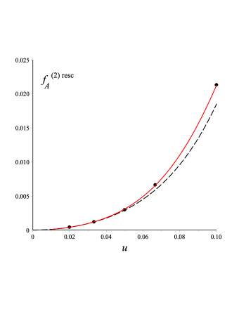
Figure 3: The data points for $f_{A}^{(2)\rm resc}$, the theoretical PN prediction (dashed curve) and the fit $f_{A}^{(2)\rm resc,fit}(u)=f_{A}^{(2)\rm resc,PN}(u)+(c_{1}+c_{2}\ln(u))u^{6}$ where $c_{1}=-24303.04$ and $c_{2}=-11754.74$.[The accuracy of the fit is found to be $2.30\times 10^{-4}$.]

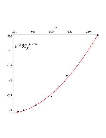
Figure 4: The data points for the rescaled quantity $\frac{1}{u^{3}}\delta G_{S}^{(4)\rm resc}(u)$ for which no theoretical prediction is available. The solid curve superposed to the points corresponds to a (quadratic) fit by the function $262.1643u^{2}+0.2878u-3.1256$.

VII Conclusions

Let us summarize our main results:

We derived the very simple relation Eq. (9) between the GSF correction $\delta z_{1}$ to the redshift (considered as a function of the orbital frequency) and the $O(m_{1}^{2})$ contribution to the two-body Hamiltonian (considered as a function of phase space variables). The latter relation then implied the simple relation (22) between $\delta z_{1}$ and the $O(\nu)$ contributions to the EOB coupling functions $A$ and $G_{S}$.

We analytically computed the PN expansion of $\delta z_{1}$ (or, equivalently, $\delta U=-\delta z_{1}/z_{1}^{2}$) up to order $O(u^{9.5})$ included and $O(\hat{a}^{4})$ included. See Eqs. (III). We then converted the latter expansions (using Eq. (22)) into correspondingly accurate PN expansions of the $O(\nu)$ corrections $\delta A$, $\delta G_{S}$ to the EOB coupling function $A,G_{S}$. The latter results represent drastic improvements in our knowledge of the spin-dependent interactions encoded within the EOB potentials $A$ and $G_{S}$.

Going beyond PN expansions (whose validity is a priori limited to the weak-field domain $u\ll 1$), we showed how to extract the numerical values of $\delta A$ and $\delta G_{S}$ in the strong-field domain $u=O(1)$ from the numerical GSF calculations of $\delta z_{1}$ Shah:2012gu . See Eqs. (47), (48) and Tables 1 and 2. We then compared the latter numerical results to our high-accuracy PN expansions and found excellent agreement when $u\ll 1$, and a good agreement ($\sim 10^{-3}$) up to $u=0.20$ (corresponding to $r_{0}=5M$).

Let us finally discuss what is probably the physically most important result of the present work. It concerns the main EOB spin-orbit coupling function $G_{S}$. Both our analytical results and our GSF-extracted numerical data show that the rescaled GSF correction $\delta G_{S}^{\rm resc}(u,\hat{a})$ significantly increases from its value $1$ at large separations $(u\to 0)$ to values of order $5$ at separations of order $r_{0}\simeq 10M$ (i.e. $u\simeq 0.1$). However, the LO rescaling factor used for $\delta G_{S}$ is negative, and equal to $-\frac{5}{8}u^{4}$. This means that the GSF correction tends to diminish the value of the total spin-orbit coupling. This confirms what was found in the previous (less accurate) PN calculations Damour:2008qf ; Nagar:2011fx ; Barausse:2011ys . Let us consider for simplicity the $\hat{a}\to 0$ limit of $G_{S}$ and work with the Kerr-rescaled spin-orbit coupling

$$\hat{G}_{S}(u,\nu,\hat{a}_{1},\hat{a}_{2}) = \frac{G_{S}(r,m_{1},m_{2},S_{1},S_{2})}{G_{S}^{\rm Kerr}(r,m_{1}+m_{2},a_{1}+a_{2})}$$ (50)

$$= 1+\frac{\delta G_{S}}{G_{S}^{\rm Kerr}}$$

(taken for $S_{1}=0=S_{2}$). The current (combined PN and GSF) knowledge of the latter function is

$$\hat{G}_{S}(u,\nu,0,0) = 1-\frac{5}{16}u\delta G_{S}^{(0){\rm resc}}(u)-\frac{1}{16}\nu^{2}u^{2}\varphi_{1}(u)$$

$$+ O(\nu^{3})$$

$$= \left(1+\frac{5}{16}u\delta G_{S}^{(0){\rm resc}}(u)\right.$$

$$\left.+\frac{41}{256}\nu^{2}u^{2}\varphi_{2}(u)+O(\nu^{3})\right)^{-1}\,,$$

where $\varphi_{n}(u)=1+O(u)$ denotes a generic PN correction factor. In the second equation we have used an inverse resummation of $\hat{G}_{S}$ as found useful in recent EOB work. Damour and Nagar Damour:2014sva have a provided an effective expression for $1/\hat{G}_{S}(u,\nu,0,0)$, parametrized by a constant $c_{3}$ as indicated below

$$[\hat{G}_{S}(u,\nu,0,0)]^{-1} = 1+\frac{5}{16}\nu u\left(1+\frac{102}{5}u\right)$$ (52)

$$+c_{3}\nu u^{3}+\frac{41}{256}\nu^{2}u^{2}\,.$$

Using our result, Eq.(45), for $\delta G_{S}^{(0){\rm resc}}(u)$ we can define an effective function of $u$, $c_{3}^{\rm eff}=c_{3}^{\rm eff}(u)$, such that the replacement $c_{3}\to c_{3}^{\rm eff}(u)$ in (52) is consistent with our full PN-expanded result. The value at $u=0$ of this $c_{3}^{\rm eff}(u)$ is found to be

$$c_{3}^{\rm eff}(0)=\frac{80399}{2304}-\frac{241}{384}\pi^{2}\approx 28.7012\,.$$ (53)

One finds that after an initial small decrease from $c_{3}(0)=28.7012$ to $c_{3}(0.0041)=28.6175$, $c_{3}(u)$ then monotonically increases with $u$. It reaches the numerically calibrated value of Refs. Damour:2014sva ; Nagar:2015xqa , namely $c_{3}^{\rm calibrated}=44.786477$, at $u=0.1593$ and then continues increasing towards large values (e.g. $c_{3}(0.5)=441.3976$). The inverse-resummed function $\hat{G}_{S}(u,\nu,0,0)$ defined by inserting our result in the second equation (VII) (with $\varphi_{2}(u)=1$ and $O(\nu^{2})\to 0$) is shown in Fig. 5 for $\nu=0.25$ and is compared to the calibrated result of Damour:2014sva ; Nagar:2015xqa . Note that our results predict a faster fall-off of $\hat{G}_{S}$ in the strong-field domain. It will be interesting to explore the EOB application of this finding.

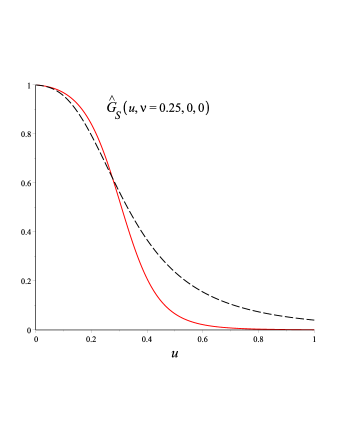
Figure 5: The quantity $\hat{G}_{S}(u,\nu,0,0)$ used in Damour-Nagar (dashed curve) Damour:2014sva as well as the present determination (solid curve) are compared in the case $\nu=0.25$.

Appendix A The Kerr case: an overview

In the test-mass limit ($S_{1}=0=m_{1}$), i.e. in the Kerr case (with mass $m_{2}$ and spin $S_{2}$), the effective Hamiltonian reads

$$\hat{H}_{\rm eff}^{(0)}=\sqrt{A_{K}(1+p_{\phi}^{2}u_{cK}^{2})}+2u_{K}u_{cK}^{2}p_{\phi}\hat{a}_{2}\,,$$ (54)

where $u_{K}\equiv m_{2}/r$, $\hat{a}_{2}=a_{2}/m_{2}=S_{2}/m_{2}^{2}$ and

$$A_{K}(u_{K},\hat{a}_{2})=\frac{1-4u_{cK}^{2}}{1+2u_{K}}\,,\qquad G_{S}^{K}(u_{K},\hat{a}_{2})=2u_{K}u_{cK}^{2}\,,$$ (55)

with

$$r_{cK}(r,m_{2},\hat{a}_{2})^{2} = r^{2}+a_{2}^{2}+\frac{2m_{2}a_{2}^{2}}{r}$$

$$= \frac{m_{2}^{2}}{u_{K}^{2}}\left(1+\hat{a}_{2}^{2}u_{K}^{2}+2\hat{a}_{2}u_{K}^{3}\right)$$

$$u_{cK}(u_{K},\hat{a}_{2}) = \frac{u_{K}}{\sqrt{1+\hat{a}_{2}^{2}u_{K}^{2}(1+2u_{K})}}\,.$$ (56)

Note also the expression of $A_{K}$ in terms of the Boyer-Lindquist coordinate $u_{K}=m_{2}/r$:

$$A_{K}(u_{K}) = 1-2u_{K}+\frac{4\hat{a}_{2}^{2}u_{K}^{4}}{1+\hat{a}_{2}^{2}u_{K}^{2}(1+2u_{K})}$$ (57)

$$= 1-2u_{K}+4\hat{a}_{2}^{2}u_{K}^{2}u_{cK}^{2}$$

The redshift $z_{1}=\partial H_{\rm eff}/\partial\mu$, as a function of $u_{K}$ (hereafter we simply denote $u_{K}$ by $u$ and $u_{cK}$ by $u_{c}$) and $p_{\phi}$, reads

$$z_{1}(u,p_{\phi},\hat{a}_{2})=\frac{A_{K}(u,\hat{a}_{2})}{\sqrt{A_{K}(u,\hat{a}_{2})(1+p_{\phi}^{2}u_{c}(u,\hat{a}_{2})^{2})}}=\sqrt{\frac{A_{K}}{Q_{K}}}\,,$$ (58)

where

$$Q_{K}=1+p_{\phi}^{2}u_{c}(u,\hat{a}_{2})^{2}\,.$$ (59)

The circular value of the (dimensionless) angular momentum is

$$p_{\phi}^{K}(u,\hat{a}_{2})=\frac{1-2\hat{a}_{2}u^{3/2}+\hat{a}_{2}^{2}u^{2}}{\sqrt{u}\sqrt{1-3u+2\hat{a}_{2}u^{3/2}}}\,.$$ (60)

The corresponding energy per unit mass, $\hat{E}=\hat{H}_{\rm eff}$, reads

$$\hat{E}(u,\hat{a}_{2})=\frac{1-2u+\hat{a}_{2}u^{3/2}}{\sqrt{1-3u+2\hat{a}_{2}u^{3/2}}}\,.$$ (61)

Substituting $p_{\phi}=p_{\phi}^{K}(u,\hat{a}_{2})$ in the above expression for $z_{1}^{K}$ yields the following “on shell” relation

$$z_{1}^{K}(u,\hat{a}_{2})=\frac{\sqrt{1-3u+2\hat{a}_{2}u^{3/2}}}{1+\hat{a}_{2}u^{3/2}}\,.$$ (62)

The circular expression for the angular frequency parameter $m_{2}\Omega^{K}=\partial\hat{H}_{\rm eff}/\partial p_{\phi}$ (as a function of $u$ after using $p_{\phi}=p_{\phi}^{K}(u,\hat{a}_{2})$ given in (60)) is (Kepler’s law, for a Kerr black hole)

$$m_{2}\Omega^{K}(u,\hat{a}_{2}) = \frac{u^{3/2}}{1+\hat{a}_{2}u^{3/2}}$$ (63)

$$= \left(\hat{a}_{2}+u^{-3/2}\right)^{-1}\,.$$

It is worth to note the following relations

$$m_{2}\Omega^{K} = \hat{a}_{2}G_{S}^{K}+\frac{A_{K}p_{\phi}^{K}u_{c}^{2}}{\sqrt{A_{K}(1+p_{\phi}^{K}{}^{2}u_{c}^{2})}}$$ (64)

$$= \hat{a}_{2}G_{S}^{K}+\sqrt{\frac{A_{K}}{Q_{K}}}p_{\phi}^{K}u_{c}^{2}$$

$$= \hat{a}_{2}G_{S}^{K}+z_{1}^{K}p_{\phi}^{K}u_{c}^{2}=u_{c}^{2}\left(2u\hat{a}_{2}+z_{1}^{K}p_{\phi}^{K}\right)\,.$$

Defining

$$\Omega^{\prime}\equiv\frac{\Omega}{1-a_{2}\Omega}\,,\qquad m_{2}\Omega^{\prime}\equiv\frac{m_{2}\Omega}{1-\hat{a}_{2}m_{2}\Omega}\,,$$ (66)

one finds that this modified frequency satisfies the usual Kepler law

$$m_{2}\Omega^{\prime}=u^{3/2}\,.$$ (67)

In other words, the modified dimensionless frequency parameter

$$y^{\prime}\equiv(m_{2}\Omega^{\prime})^{2/3}\,,$$ (68)

is such that

$$u^{\rm circ}=y^{\prime}\,.$$ (69)

The explicit transformation $y\to y^{\prime}$ reads

$$y^{\prime} = \frac{y}{(1-\hat{a}_{2}y^{3/2})^{2/3}}$$ (70)

$$= y\left[1+\frac{2}{3}{\hat{a}}_{2}y^{3/2}+\frac{5}{9}{\hat{a}}_{2}^{2}y^{3}+O(y^{9/2})\right]\,.$$

The inverse of this transformation is obtained by exchanging $y^{\prime}$ and $y$ and ${\hat{a}}_{2}\to-{\hat{a}}_{2}$, namely

$$y=\frac{y^{\prime}}{(1+\hat{a}_{2}y^{\prime}{}^{3/2})^{2/3}}\,.$$ (71)

Expressing $z_{1}(y^{\prime})$ in terms of $y$ leads to

$$z_{1}^{K}(y) = \frac{(1-3y^{\prime}+2\hat{a}_{2}y^{\prime 3/2})^{1/2}}{1+\hat{a}_{2}y^{\prime 3/2}}\qquad{\rm(exact)}$$ (72)

$$= \sqrt{1-3y}+\hat{a}_{2}\left(2y^{5/2}+3y^{7/2}+\frac{27}{4}y^{9/2}\right.$$

$$\left.+\frac{135}{8}y^{11/2}+\frac{2835}{64}y^{13/2}+\frac{15309}{128}y^{15/2}\right)$$

$$+O(y^{8},\hat{a}_{2}^{2})\,.$$

Note that the equation

$$1-3y^{\prime}+2\hat{a}_{2}y^{\prime 3/2}=0$$ (73)

defines the light-ring for co-rotating circular geodesics. Table 7 lists light-ring values of $y^{\prime}$ for representative values of $\hat{a}_{2}$.

Table 7: Light-ring position $y^{\prime}$ for fixed values of $\hat{a}_{2}$.

$\hat{a}_{2}$	$y^{\prime}$
-1.0	0.25
-0.9	0.2557369509
-0.7	0.2684314963
-0.5	0.2831185829
0	0.3333333333
0.5	0.4260220478
0.7	0.4966885468
0.9	0.6419084184
1.0	1.0

Finally, the explicit expression, in a Kerr background, of the $G_{S_{*}}$-type spin-orbit coupling (defined in an arbitrary equatorial metric by Eq. (21)) reads

$$G_{S_{*}}^{\rm Kerr}(u,\hat{a}) = z_{1}^{K}u_{c}^{2}\left[1-\sqrt{A}(1-\hat{a}^{2}u^{3})\right]$$ (74)

$$+ \frac{u_{c}^{4}[(1+\hat{a}^{2}u^{2})^{2}-4\hat{a}^{2}u^{3}]}{u(1+\sqrt{Q_{K}})}\,.$$

Note that this quantity differs from the ratio $R\equiv m_{2}\Omega_{\rm SO}^{K}/p_{\phi}^{K}$ between the dimensionless spin-orbit precession angular velocity Iyer:1993qa

$$m_{2}\Omega_{\rm SO}^{K}=\frac{1-\sqrt{1-3u+2\hat{a}_{2}u^{3/2}}}{\hat{a}_{2}+u^{-3/2}}$$ (75)

and the dimensionless angular momentum $p_{\phi}^{K}$. Indeed, the structure of the effective Hamiltonian (12) shows that $\Omega_{\rm SO}^{K}=\lim_{S_{1}\to 0}\partial H_{\rm eff}/\partial S_{1}$ is (in the test-mass limit $m_{1}\to 0$ with $S_{1}/m_{1}$ fixed) the sum of two contributions: a contribution $\propto G_{S_{*}}p_{\phi}$ and a contribution coming from the $S_{1}$ derivative of the orbital effective Hamiltonian $\sqrt{A(\mu^{2}+L^{2}/r_{c}^{2})}$ [the latter being even in spins, and therefore notably containing relevant terms of the form $\sim S_{1}(S_{2}+S_{2}^{3}+\ldots)$]. In the Schwarzschild limit, $G_{S_{*}}^{\rm Kerr}$ reduces to

$$G_{S_{*}}^{\rm Schw}(u)=\frac{3u^{3}}{1+\frac{1}{\sqrt{1-3u}}}\,.$$ (76)

Acknowledgments

We are grateful to Abhay Shah for many informative discussions and for communicating us the corrected version of Table III in Ref. Shah:2012gu . D.B. thanks the Italian INFN (Naples) for partial support and IHES for hospitality during the development of this project. All the authors are grateful to ICRANet for partial support.

References

(1)
A. Buonanno and T. Damour,
“Effective one-body approach to general relativistic two-body dynamics,”
Phys. Rev. D 59, 084006 (1999)
[gr-qc/9811091].
(2)
A. Buonanno and T. Damour,
“Transition from inspiral to plunge in binary black hole coalescences,”
Phys. Rev. D 62, 064015 (2000)
[gr-qc/0001013].
(3)
T. Damour, P. Jaranowski and G. Schaefer,
“On the determination of the last stable orbit for circular general relativistic binaries at the third postNewtonian approximation,”
Phys. Rev. D 62, 084011 (2000)
[gr-qc/0005034].
(4)
T. Damour,
“Coalescence of two spinning black holes: an effective one-body approach,”
Phys. Rev. D 64, 124013 (2001)
[gr-qc/0103018].
(5)
G. Schaefer,
“Post-Newtonian methods: Analytic results on the binary problem,”
Fundam. Theor. Phys. 162, 167 (2011)
[arXiv:0910.2857 [gr-qc]].
(6)
L. Blanchet,
“Gravitational Radiation from Post-Newtonian Sources and Inspiralling Compact Binaries,”
Living Rev. Rel. 17, 2 (2014)
[arXiv:1310.1528 [gr-qc]].
(7)
L. Barack,
“Gravitational self force in extreme mass-ratio inspirals,”
Class. Quant. Grav. 26, 213001 (2009)
[arXiv:0908.1664 [gr-qc]].
(8)
E. Poisson, A. Pound and I. Vega,
“The Motion of point particles in curved spacetime,”
Living Rev. Rel. 14, 7 (2011)
[arXiv:1102.0529 [gr-qc]].
(9)
S. L. Detweiler,
“A Consequence of the gravitational self-force for circular orbits of the Schwarzschild geometry,”
Phys. Rev. D 77, 124026 (2008)
[arXiv:0804.3529 [gr-qc]].
(10)
L. Blanchet, S. L. Detweiler, A. Le Tiec and B. F. Whiting,
“Post-Newtonian and Numerical Calculations of the Gravitational Self-Force for Circular Orbits in the Schwarzschild Geometry,”
Phys. Rev. D 81, 064004 (2010)
[arXiv:0910.0207 [gr-qc]].
(11)
T. Damour,
“Gravitational Self Force in a Schwarzschild Background and the Effective One Body Formalism,”
Phys. Rev. D 81, 024017 (2010)
[arXiv:0910.5533 [gr-qc]].
(12)
L. Blanchet, S. L. Detweiler, A. Le Tiec and B. F. Whiting,
“High-Order Post-Newtonian Fit of the Gravitational Self-Force for Circular Orbits in the Schwarzschild Geometry,”
Phys. Rev. D 81, 084033 (2010)
[arXiv:1002.0726 [gr-qc]].
(13)
L. Barack, T. Damour and N. Sago,
“Precession effect of the gravitational self-force in a Schwarzschild spacetime and the effective one-body formalism,”
Phys. Rev. D 82, 084036 (2010)
[arXiv:1008.0935 [gr-qc]].
(14)
T. S. Keidl, A. G. Shah, J. L. Friedman, D. H. Kim and L. R. Price,
“Gravitational Self-force in a Radiation Gauge,”
Phys. Rev. D 82, no. 12, 124012 (2010)
[Phys. Rev. D 90, no. 10, 109902 (2014)]
[arXiv:1004.2276 [gr-qc]].
(15)
A. Le Tiec, E. Barausse and A. Buonanno,
“Gravitational Self-Force Correction to the Binding Energy of Compact Binary Systems,”
Phys. Rev. Lett. 108, 131103 (2012)
[arXiv:1111.5609 [gr-qc]].
(16)
E. Barausse, A. Buonanno and A. Le Tiec,
“The complete non-spinning effective-one-body metric at linear order in the mass ratio,”
Phys. Rev. D 85, 064010 (2012)
[arXiv:1111.5610 [gr-qc]].
(17)
A. G. Shah, J. L. Friedman and T. S. Keidl,
“EMRI corrections to the angular velocity and redshift factor of a mass in circular orbit about a Kerr black hole,”
Phys. Rev. D 86, 084059 (2012)
[arXiv:1207.5595 [gr-qc]].
(18)
S. Akcay, L. Barack, T. Damour and N. Sago,
“Gravitational self-force and the effective-one-body formalism between the innermost stable circular orbit and the light ring,”
Phys. Rev. D 86, 104041 (2012)
[arXiv:1209.0964 [gr-qc]].
(19)
D. Bini and T. Damour,
“Analytical determination of the two-body gravitational interaction potential at the fourth post-Newtonian approximation,”
Phys. Rev. D 87, no. 12, 121501 (2013)
[arXiv:1305.4884 [gr-qc]].
(20)
S. R. Dolan, N. Warburton, A. I. Harte, A. L. Tiec, B. Wardell and L. Barack,
“Gravitational self-torque and spin precession in compact binaries,”
Phys. Rev. D 89, 064011 (2014)
[arXiv:1312.0775 [gr-qc]].
(21)
A. G. Shah, J. L. Friedman and B. F. Whiting,
“Finding high-order analytic post-Newtonian parameters from a high-precision numerical self-force calculation,”
arXiv:1312.1952 [gr-qc].
(22)
D. Bini and T. Damour,
“High-order post-Newtonian contributions to the two-body gravitational interaction potential from analytical gravitational self-force calculations,”
Phys. Rev. D 89, no. 6, 064063 (2014)
[arXiv:1312.2503 [gr-qc]].
(23)
D. Bini and T. Damour,
“Analytic determination of the eight-and-a-half post-Newtonian self-force contributions to the two-body gravitational interaction potential,”
Phys. Rev. D 89, no. 10, 104047 (2014)
[arXiv:1403.2366 [gr-qc]].
(24)
D. Bini and T. Damour,
“Two-body gravitational spin-orbit interaction at linear order in the mass ratio,”
Phys. Rev. D 90, no. 2, 024039 (2014)
[arXiv:1404.2747 [gr-qc]].
(25)
S. R. Dolan, P. Nolan, A. C. Ottewill, N. Warburton and B. Wardell,
“Tidal invariants for compact binaries on quasicircular orbits,”
Phys. Rev. D 91, no. 2, 023009 (2015)
[arXiv:1406.4890 [gr-qc]].
(26)
D. Bini and T. Damour,
“Gravitational self-force corrections to two-body tidal interactions and the effective one-body formalism,”
Phys. Rev. D 90, no. 12, 124037 (2014)
[arXiv:1409.6933 [gr-qc]].
(27)
D. Bini and T. Damour,
“Analytic determination of high-order post-Newtonian self-force contributions to gravitational spin precession,”
Phys. Rev. D 91, no. 6, 064064 (2015)
[arXiv:1503.01272 [gr-qc]].
(28)
D. Bini and T. Damour,
“Detweiler’s gauge-invariant redshift variable: analytic determination of the nine and nine-and-a-half post-Newtonian self-force contributions,”
Phys. Rev. D 91, 064050 (2015)
arXiv:1502.02450 [gr-qc].
(29)
C. Kavanagh, A. C. Ottewill and B. Wardell,
“Analytical high-order post-Newtonian expansions for extreme mass ratio binaries,”
Phys. Rev. D 92, no. 8, 084025 (2015)
[arXiv:1503.02334 [gr-qc]].
(30)
A. Buonanno, Y. Pan, H. P. Pfeiffer, M. A. Scheel, L. T. Buchman and L. E. Kidder,
“Effective-one-body waveforms calibrated to numerical relativity simulations: Coalescence of non-spinning, equal-mass black holes,”
Phys. Rev. D 79, 124028 (2009)
[arXiv:0902.0790 [gr-qc]].
(31)
A. Le Tiec, A. H. Mroue, L. Barack, A. Buonanno, H. P. Pfeiffer, N. Sago and A. Taracchini,
“Periastron Advance in Black Hole Binaries,”
Phys. Rev. Lett. 107, 141101 (2011)
[arXiv:1106.3278 [gr-qc]].
(32)
T. Damour, A. Nagar, D. Pollney and C. Reisswig,
“Energy versus Angular Momentum in Black Hole Binaries,”
Phys. Rev. Lett. 108, 131101 (2012)
[arXiv:1110.2938 [gr-qc]].
(33)
T. Damour, A. Nagar and S. Bernuzzi,
“Improved effective-one-body description of coalescing nonspinning black-hole binaries and its numerical-relativity completion,”
Phys. Rev. D 87, 084035 (2013)
[arXiv:1212.4357 [gr-qc]].
(34)
I. Hinder, A. Buonanno, M. Boyle, Z. B. Etienne, J. Healy, N. K. Johnson-McDaniel, A. Nagar and H. Nakano et al.,
“Error-analysis and comparison to analytical models of numerical waveforms produced by the NRAR Collaboration,”
Class. Quant. Grav. 31, 025012 (2014)
[arXiv:1307.5307 [gr-qc]].
(35)
Y. Pan, A. Buonanno, A. Taracchini, L. E. Kidder, A. H. Mrou , H. P. Pfeiffer, M. A. Scheel and B. Szil gyi,
“Inspiral-merger-ringdown waveforms of spinning, precessing black-hole binaries in the effective-one-body formalism,”
Phys. Rev. D 89, 084006 (2014)
[arXiv:1307.6232 [gr-qc]].
(36)
A. Taracchini et al.,
“Effective-one-body model for black-hole binaries with generic mass ratios and spins,”
Phys. Rev. D 89, 061502 (2014)
[arXiv:1311.2544 [gr-qc]].
(37)
Y. Pan et al.,
“Stability of nonspinning effective-one-body model in approximating two-body dynamics and gravitational-wave emission,”
Phys. Rev. D 89, 061501 (2014)
[arXiv:1311.2565 [gr-qc]].
(38)
T. Damour, F. Guercilena, I. Hinder, S. Hopper, A. Nagar and L. Rezzolla,
“Strong-Field Scattering of Two Black Holes: Numerics Versus Analytics,”
arXiv:1402.7307 [gr-qc].
(39)
T. Damour and A. Nagar,
“New effective-one-body description of coalescing nonprecessing spinning black-hole binaries,”
Phys. Rev. D 90, no. 4, 044018 (2014)
[arXiv:1406.6913 [gr-qc]].
(40)
A. G. Shah, private communication.
(41)
A. G. Shah, Capra conference 2015.
(42)
A. G. Shah, talk delivered at the MG14.
(43)
M. van de Meent and A. G. Shah,
“Metric perturbations produced by eccentric equatorial orbits around a Kerr black hole,”
Phys. Rev. D 92, 064025 (2015)
[arXiv:1506.04755 [gr-qc]].
(44)
A. Le Tiec, L. Blanchet and B. F. Whiting,
“The First Law of Binary Black Hole Mechanics in General Relativity and Post-Newtonian Theory,”
Phys. Rev. D 85, 064039 (2012)
[arXiv:1111.5378 [gr-qc]].
(45)
L. Blanchet, A. Buonanno and A. Le Tiec,
“First law of mechanics for black hole binaries with spins,”
Phys. Rev. D 87, no. 2, 024030 (2013)
[arXiv:1211.1060 [gr-qc]].
(46)
A. L. Tiec,
“First Law of Mechanics for Compact Binaries on Eccentric Orbits,”
arXiv:1506.05648 [gr-qc].
(47)
T. Damour, P. Jaranowski and G. Schaefer,
“Hamiltonian of two spinning compact bodies with next-to-leading order gravitational spin-orbit coupling,”
Phys. Rev. D 77, 064032 (2008)
[arXiv:0711.1048 [gr-qc]].
(48)
S. Balmelli and T. Damour,
“A new effective-one-body Hamiltonian with next-to-leading order spin-spin coupling,”
arXiv:1509.08135 [gr-qc].
(49)
E. Barausse and A. Buonanno,
“An Improved effective-one-body Hamiltonian for spinning black-hole binaries,”
Phys. Rev. D 81, 084024 (2010)
[arXiv:0912.3517 [gr-qc]].
(50)
S. Mano, H. Suzuki and E. Takasugi,
“Analytic solutions of the Regge-Wheeler equation and the postMinkowskian expansion,”
Prog. Theor. Phys. 96, 549 (1996)
[gr-qc/9605057].
(51)
S. Mano, H. Suzuki and E. Takasugi,
“Analytic solutions of the Teukolsky equation and their low frequency expansions,”
Prog. Theor. Phys. 95, 1079 (1996)
[gr-qc/9603020].
(52)
L. Blanchet, G. Faye and B. F. Whiting,
“Half-integral conservative post-Newtonian approximations in the redshift factor of black hole binaries,”
Phys. Rev. D 89, no. 6, 064026 (2014)
[arXiv:1312.2975 [gr-qc]].
(53)
T. Damour, P. Jaranowski and G. Schäfer,
“Fourth post-Newtonian effective one-body dynamics,”
Phys. Rev. D 91, no. 8, 084024 (2015)
[arXiv:1502.07245 [gr-qc]].
(54)
L. Blanchet and T. Damour,
“Tail Transported Temporal Correlations in the Dynamics of a Gravitating System,”
Phys. Rev. D 37, 1410 (1988).
(55)
N. K. Johnson-McDaniel, A. G. Shah and B. F. Whiting,
“Experimental mathematics meets gravitational self-force,”
Phys. Rev. D 92, no. 4, 044007 (2015)
[arXiv:1503.02638 [gr-qc]].
(56)
T. Damour, P. Jaranowski and G. Schaefer,
“Effective one body approach to the dynamics of two spinning black holes with next-to-leading order spin-orbit coupling,”
Phys. Rev. D 78, 024009 (2008)
[arXiv:0803.0915 [gr-qc]].
(57)
A. Nagar,
“Effective one body Hamiltonian of two spinning black-holes with next-to-next-to-leading order spin-orbit coupling,”
Phys. Rev. D 84, 084028 (2011)
[Phys. Rev. D 88, no. 8, 089901 (2013)]
[arXiv:1106.4349 [gr-qc]].
(58)
E. Barausse and A. Buonanno,
“Extending the effective-one-body Hamiltonian of black-hole binaries to include next-to-next-to-leading spin-orbit couplings,”
Phys. Rev. D 84, 104027 (2011)
[arXiv:1107.2904 [gr-qc]].
(59)
S. Balmelli and P. Jetzer,
“Effective-one-body Hamiltonian with next-to-leading order spin-spin coupling for two nonprecessing black holes with aligned spins,”
Phys. Rev. D 87, no. 12, 124036 (2013)
[Erratum-ibid. D 90, no. 8, 089905 (2014)]
[arXiv:1305.5674 [gr-qc]].
(60)
A. Nagar, T. Damour, C. Reisswig and D. Pollney,
“Energetics and phasing of nonprecessing spinning coalescing black hole binaries,”
arXiv:1506.08457 [gr-qc].
(61)
B. R. Iyer and C. V. Vishveshwara,
“The Frenet-Serret description of gyroscopic precession,”
Phys. Rev. D 48, 5706 (1993)
[gr-qc/9310019].