Maslov-type indices and linear stability of elliptic Euler solutions of the three-body problem

Abstract

In this paper, we use the central configuration coordinate decomposition to study the linearized Hamiltonian system near the $3$-body elliptic Euler solutions. Then using the Maslov-type $\omega$-index theory of symplectic paths and the theory of linear operators we compute the ${\omega}$-indices and obtain certain properties of linear stability of the Euler elliptic solutions of the classical three-body problem.

Keywords: planar three-body problem, Euler solution, linear stability, ${\omega}$-index theory, perturbations of linear operators.

AMS Subject Classification: 58E05, 37J45, 34C25

1 Introduction and main results

In 1767, Euler ([2]) discovered some celebrated periodic solutions, now named after him, to the planar three-body problem, namely the three bodies are collinear at any instant of the motion and at the same time each body travels along a specific Keplerian elliptic orbit about the center of masses of the system. All these orbits are homographic solutions. When $0\leq e<1$, the Keplerian orbit is elliptic, we call such elliptic Euler (Lagrangian) solutions Euler (Lagrangian) elliptic relative equilibria. Specially when $e=0$, the Keplerian elliptic motion becomes circular motion and then all the three bodies move around the center of masses along circular orbits with the same frequency, which are called Euler (Lagrangian) relative equilibria traditionally. In this paper, we study the Maslov-type and Morse indices of such elliptic Euler solutions which are closely related to their linear stability.

Denote by $q_{1},q_{2},q_{3}\in{\bf R}^{2}$ the position vectors of three particles with masses $m_{1},m_{2},m_{3}>0$ respectively. Then the system of equations for this problem is

$$m_{i}\ddot{q}_{i}=\frac{\partial U}{\partial q_{i}},\qquad{\rm for}\quad i=1,2,3,$$ (1.1)

where $U(q)=U(q_{1},q_{2},q_{3})=\sum_{1\leq i<j\leq 3}\frac{m_{i}m_{j}}{|q_{i}-q_{j}|}$ is the potential or force function by using the standard norm $|\cdot|$ of vector in ${\bf R}^{2}$.

Note that $2\pi$-periodic solutions of this problem correspond to critical points of the action functional

$$\mathcal{A}(q)=\int_{0}^{2\pi}\left[\sum_{i=1}^{3}\frac{m_{i}|\dot{q}_{i}(t)|^{2}}{2}+U(q(t))\right]dt$$

defined on the loop space $W^{1,2}({\bf R}/2\pi{\bf Z},\hat{\mathcal{X}})$, where

$$\hat{\mathcal{X}}:=\left\{q=(q_{1},q_{2},q_{3})\in({\bf R}^{2})^{3}\,\,\left|\,\,\sum_{i=1}^{3}m_{i}q_{i}=0,\,\,q_{i}\neq q_{j},\,\,\forall i\neq j\right.\right\}$$

is the configuration space of the planar three-body problem.

Letting $p_{i}=m_{i}\dot{q}_{i}\in{\bf R}^{2}$ for $1\leq i\leq 3$, then (1.1) is transformed to a Hamiltonian system

$$\dot{p}_{i}=-\frac{\partial H}{\partial q_{i}},\,\,\dot{q}_{i}=\frac{\partial H}{\partial p_{i}},\qquad{\rm for}\quad i=1,2,3,$$ (1.2)

with Hamiltonian function

$$H(p,q)=H(p_{1},p_{2},p_{3},q_{1},q_{2},q_{3})=\sum_{i=1}^{3}\frac{|p_{i}|^{2}}{2m_{i}}-U(q_{1},q_{2},q_{3}).$$ (1.3)

For the planar three-body problem with masses $m_{1},m_{2},m_{3}>0$, it turns out that the stability of elliptic Euler solutions depends on two parameters, namely the mass parameter $\beta\in[0,7]$ defined below and the eccentricity $e\in[0,1)$,

$$\beta=\frac{m_{1}(3x^{2}+3x+1)+m_{3}x^{2}(x^{2}+3x+3)}{x^{2}+m_{2}[(x+1)^{2}(x^{2}+1)-x^{2}]},$$ (1.4)

where $x$ is the unique positive solution of the Euler quintic polynomial equation (2.1).

The linear stability of Lagrangian relative equilibria can be found in Gascheau ([3], 1843), Routh ([24], 1875), Danby ([1], 1964) and Roberts ([23], 2002). In 2005, Meyer and Schmidt (cf. [22]) used heavily the central configuration nature of the elliptic Lagrangian orbits and decomposed the fundamental solution of the elliptic Lagrangian orbit into two parts symplectically, one of which is the same as that of the Keplerian solution and the other is the essential part for the stability.

In 2004-2006, Martínez, Samà and Simó ([19],[20],[21]) studied the stability problem including Euler elliptic relative equilibria when $e>0$ is small enough by using normal form theory, and $e<1$ and close to $1$ enough by using blow-up technique in general homogeneous potential. They further gave a much more complete bifurcation diagram numerically and a beautiful figure was drawn there for the full $({\beta},e)$ range (cf. Figure 4 of [21]).

In [8] and [9] of 2009-2010, Hu and Sun found a new way to relate the stability problem to the iterated Morse indices. Recently, by observing new phenomenons and discovering new properties of elliptic Lagrangian solution, in the joint paper [5] of Hu, Long and Sun, the linear stability of elliptic Lagrangian solution is completely solved analytically by index theory (cf. [13] and [16]) and the new results are related directly to $(\beta,e)$ in the full parameter rectangle.

In the current paper, for the elliptic Euler solutions, following the central configuration coordinate method of Meyer and Schmidt in [22] and the index method used by Hu, Long and Sun in [5], we linearized the Hamiltonian system (1.2)-(1.3) near the Euler elliptic solution in Section 2 below. Here the linearized Hamiltonian system can also be decomposed into two parts symplectically, one of which is the same as that of the Kepler solutions, and the other is a $4$-dimensional Hamiltonian system whose fundamental solution is the essential part for the stability of the elliptic Euler solutions. However, the essential part here is very different from that of the Lagrangian elliptic solutions in [22] and [5]. This essential part is denoted by $\gamma_{\beta,e}(t)$ for $t\in[0,2\pi]$, which is a path in ${\rm Sp}(4)$ starting from the identity. Then we use index theory to compute the Maslov-type indices of ${\gamma}_{{\beta},e}$ and determine its stability properties.

Following [14] and [16], for any $\omega\in{\bf U}=\{z\in{\bf C}\;|\;|z|=1\}$ we can define a real function $D_{\omega}(M)=(-1)^{n-1}\overline{{\omega}}^{n}det(M-{\omega}I_{2n})$ for any $M$ in the symplectic group ${\rm Sp}(2n)$. Then we can define ${\rm Sp}(2n)_{{\omega}}^{0}=\{M\in{\rm Sp}(2n)\,|\,D_{{\omega}}(M)=0\}$ and ${\rm Sp}(2n)_{{\omega}}^{\ast}={\rm Sp}(2n)\setminus{\rm Sp}(2n)_{{\omega}}^{0}$. The orientation of ${\rm Sp}(2n)_{{\omega}}^{0}$ at any of its point $M$ is defined to be the positive direction $\frac{d}{dt}Me^{tJ}|_{t=0}$ of the path $Me^{tJ}$ with $t>0$ small enough. Let $\nu_{{\omega}}(M)=\dim_{{\bf C}}\ker_{{\bf C}}(M-{\omega}I_{2n})$. Let $\mathcal{P}_{2\pi}(2n)=\{{\gamma}\in C([0,2\pi],{\rm Sp}(2n))\;|\;{\gamma}(0)=I\}$ and $\xi(t)={\rm diag}(2-\frac{t}{2\pi},(2-\frac{t}{2\pi})^{-1})$ for $0\leq t\leq 2\pi$.

Given any two $2m_{k}\times 2m_{k}$ matrices of square block form $M_{k}=\left(\matrix{A_{k}&B_{k}\cr C_{k}&D_{k}\cr}\right)$ with $k=1,2$, the symplectic sum of $M_{1}$ and $M_{2}$ is defined (cf. [14] and [16]) by the following $2(m_{1}+m_{2})\times 2(m_{1}+m_{2})$ matrix $M_{1}{\rm\diamond}M_{2}$:

$$M_{1}{\rm\diamond}M_{2}=\left(\matrix{A_{1}&0&B_{1}&0\cr 0&A_{2}&0&B_{2}\cr C_{1}&0&D_{1}&0\cr 0&C_{2}&0&D_{2}\cr}\right),$$

and $M^{{\rm\diamond}k}$ denotes the $k$ copy ${\rm\diamond}$-sum of $M$. For any two paths ${\gamma}_{j}\in{\cal P}_{\tau}(2n_{j})$ with $j=0$ and $1$, let ${\gamma}_{0}{\rm\diamond}{\gamma}_{1}(t)={\gamma}_{0}(t){\rm\diamond}{\gamma}_{1}(t)$ for all $t\in[0,\tau]$.

For any ${\gamma}\in\mathcal{P}_{2\pi}(2n)$ we define $\nu_{\omega}({\gamma})=\nu_{\omega}({\gamma}(2\pi))$ and

$$i_{\omega}({\gamma})=[{\rm Sp}(2n)_{\omega}^{0}:{\gamma}\ast\xi^{n}],\qquad{\rm if}\;\;{\gamma}(2\pi)\not\in{\rm Sp}(2n)_{{\omega}}^{0},$$

i.e., the usual homotopy intersection number, and the orientation of the joint path ${\gamma}\ast\xi_{n}$ is its positive time direction under homotopy with fixed end points. When ${\gamma}(2\pi)\in{\rm Sp}(2n)_{{\omega}}^{0}$, we define $i_{{\omega}}({\gamma})$ be the index of the left rotation perturbation path ${\gamma}_{-{\epsilon}}$ with ${\epsilon}>0$ small enough (cf. Def. 5.4.2 on p.129 of [16]). The pair $(i_{{\omega}}({\gamma}),\nu_{{\omega}}({\gamma}))\in{\bf Z}\times\{0,1,\ldots,2n\}$ is called the index function of ${\gamma}$ at ${\omega}$. When $\nu_{{\omega}}({\gamma})=0$ or $\nu_{{\omega}}({\gamma})>0$, the path ${\gamma}$ is called ${\omega}$-non-degenerate or ${\omega}$-degenerate respectively. For more details we refer to the Appendix 5.2 or [16].

The following three theorems describe main results proved in this paper.

Theorem 1.1

In the planar three-body problem with masses $m_{1},m_{2}$, and $m_{3}>0$, for the elliptic Euler solution $q=q_{{\beta},e}(t)=(q_{1}(t),q_{2}(t),q_{3}(t))$ with eccentricity $e$ and mass parameter $\beta$ given by (1.4), we denote by ${\gamma}_{{\beta},e}:[0,2\pi]\to{\rm Sp}(4)$ the essential part of the fundamental solution of the linearized Hamiltonian system of (1.1) at $q$. Then the following results on the Maslov-type indices of ${\gamma}_{{\beta},e}$ hold.

(i) $(i_{1}({\gamma}_{0,e}),\nu_{1}({\gamma}_{0,e}))=(0,3)$ and $(i_{{\omega}}({\gamma}_{0,e}),\nu_{{\omega}}({\gamma}_{0,e}))=(2,0)$ for ${\omega}\in{\bf U}\setminus\{1\}$.

(ii) Let

$$\hat{\beta}_{n}=\frac{n^{2}-3+\sqrt{9n^{4}-14n^{2}+9}}{4}\qquad\forall\;n\in{\bf N}.$$ (1.5)

Then

$$i_{1}({\gamma}_{{\beta},0})=\left\{\matrix{0,&{\it if}\;\;{\beta}=\hat{\beta}_{1}=0,\cr 2n+1,&{\it if}\;\;{\beta}\in(\hat{\beta}_{n},\hat{\beta}_{n+1}]\;\;{\it for}\;n\in{\bf N},\cr}\right.$$ (1.6)

$$\nu_{1}({\gamma}_{{\beta},0})=\left\{\matrix{3,&{\it if}\;\;{\beta}=\hat{\beta}_{1}=0,\cr 2,&{\it if}\;\;{\beta}=\hat{\beta}_{n},\;n\geq 2,\cr 0,&{\it if}\;\;{\beta}\in[0,+\infty)\setminus\{\hat{\beta}_{n}\;|\;n\in{\bf N}\}.\cr}\right.$$ (1.7)

(iii) Let

$$\hat{\beta}_{n+\frac{1}{2}}=\frac{(n+\frac{1}{2})^{2}-3+\sqrt{9(n+\frac{1}{2})^{4}-14(n+\frac{1}{2})^{2}+9}}{4}\qquad\forall\;n\in{\bf N}.$$ (1.8)

Then

$$i_{-1}({\gamma}_{{\beta},0})=\left\{\matrix{2,&{\it if}\;\;{\beta}\in[0,\hat{\beta}_{\frac{3}{2}}],\cr 2n,&{\it if}\;\;{\beta}\in(\hat{\beta}_{n-\frac{1}{2}},\hat{\beta}_{n+\frac{1}{2}}]\;\;{\it for}\;n\geq 2,\cr}\right.$$ (1.9)

$$\nu_{-1}({\gamma}_{{\beta},0})=\left\{\matrix{2,&{\rm if}\;\;{\beta}=\hat{\beta}_{n+\frac{1}{2}}\;{\it for}\;n\in{\bf N},\cr 0,&{\rm if}\;\;{\beta}\in[0,+\infty)\setminus\{\hat{\beta}_{n+\frac{1}{2}}\;|\;n\in{\bf N}\}.\cr}\right.$$ (1.10)

(iv) For fixed $e\in[0,1)$ and ${\omega}\in{\bf U}$, $i_{{\omega}}({\gamma}_{{\beta},e})$ is non-decreasing and tends to $+\infty$ when ${\beta}$ increases from $0$ to $+\infty$.

(v) $i_{1}({\gamma}_{{\beta},e})>0$ is odd for all $({\beta},e)\in(0,+\infty)\times[0,1)$.

(vi) $i_{1}({\gamma}_{{\beta},e})\leq 4n+2$ holds when ${\beta}<\frac{2}{3\sqrt{2}-1}(n^{2}-\frac{e}{1+e})(1-e)-1$ for any $n\in{\bf N}$.

(vii) For any $\epsilon\in(0,1)$, there exists a ${\beta}_{\epsilon}>0$ such that $\nu_{1}({\gamma}_{{\beta},e})=0$, i.e., ${\gamma}_{{\beta},e}$ is non-degenerate when $({\beta},e)\in(0,{\beta}_{\epsilon}]\times[0,1-\epsilon]$.

Remark 1.2

(i) Here we are specially interested in indices in eigenvalues $1$ and $-1$. The reason is that the major changes of the linear stability of the elliptic Euler solutions happen near the eigenvalues $1$ and $-1$, and such information is used in the next theorem to get the separation curves of the linear stability domain $[0,+\infty)\times[0,1)$ of the mass and eccentricity parameter $({\beta},e)$.

(ii) The situations of other eigenvalues ${\omega}\in{\bf U}\setminus{\bf R}$ of ${\gamma}_{{\beta},e}(2\pi)$ can be obtained by the method in Section 4 below similarly, which then yields complete understanding on the eigenvalue distribution of ${\gamma}_{{\beta},0}(2\pi)$ for all ${\beta}\geq 0$, i.e., the linear stability of the Euler relative equilibria $q_{{\beta},0}(t)$. Note that by the essential part of the linearized Hamiltonian system at the elliptic Euler solutions found in (2.35) below, $e=0$ yields an autonomous Hamiltonian system, and thus the linear stability is explicitly computable.

(iii) Note that ${\beta}\in[0,7]$ in its physical meaning. For mathematical interest and convenience, we extend the range of the parameter ${\beta}$ to $[0,\infty)$.

Theorem 1.3

Using notations in Theorem 1.1, for the elliptic Euler solution $q=q_{{\beta},e}(t)$ with eccentricity $e$ and mass parameter $\beta$ given by (1.4), the following results on the linear stability separation curves of ${\gamma}_{{\beta},e}$ in the parameter $({\beta},e)$ domain ${\Theta}=[0,+\infty)\times[0,1)$ hold. Letting

$${\Gamma}_{n} = \{({\beta}_{2n-1}(1,e),e)\;|\;e\in[0,1)\}\quad{\it with}\quad{\beta}_{2n-1}(1,e)=({\beta}_{2n}(1,e),$$

$$\Xi_{n}^{-} = \{({\beta}_{2n-1}(-1,e),e)\;|\;e\in[0,1)\},$$

$$\Xi_{n}^{+} = \{({\beta}_{2n}(-1,e),e)\;|\;e\in[0,1)\},$$

we then have the following:

(i) Starting from the point $(\hat{\beta}_{n+1},0)$ defined in (1.5) for $n\in{\bf N}$, there exists exactly one $1$-degenerate curve ${\Gamma}_{n}$ of ${\gamma}_{{\beta},e}(2\pi)$ which is perpendicular to the ${\beta}$-axis, goes up into the domain ${\Theta}$, intersects each horizontal line $e={\rm constant}$ in ${\Theta}$ precisely once for each $e\in(0,1)$, and satisfies $\nu_{1}({\gamma}_{{\beta}_{2n}(1,e),e})=2$ at such an intersection point $({\beta}_{2n}(1,e),e)\in{\Gamma}_{n}$, see Figure 1 below (cf. left figure of Figure 6 in [20]). Further more, ${\beta}_{2n}(1,e)$ is a real analytic function in $e\in[0,1)$.

(ii) Starting from the point $(\hat{\beta}_{n+1/2},0)$ defined in (1.8) for $n\in{\bf N}$, there exists exactly two $-1$-degenerate curves $\Xi_{n}^{\pm}$ of ${\gamma}_{{\beta},e}(2\pi)$ which are perpendicular to the ${\beta}$-axis, go up into the domain ${\Theta}$. Moreover, for each $e\in(0,1)$, if ${\beta}_{2n-1}(-1,e)\neq{\beta}_{2n}(-1,e)$, the two curves intersect each horizontal line $e={\rm constant}$ in ${\Theta}$ precisely once and satisfy $\nu_{1}({\gamma}_{{\beta}_{2n-1}(-1,e),e})=\nu_{1}({\gamma}_{{\beta}_{2n}(-1,e),e})=1$ at such an intersection point $({\beta}_{2n-1}(-1,e),e)\in\Xi_{n}^{-}$ and $({\beta}_{2n}(-1,e),e)\in\Xi_{n}^{+}$; if ${\beta}_{2n-1}(-1,e)={\beta}_{2n}(-1,e)$, the two curves intersect each horizontal line $e={\rm constant}$ in ${\Theta}$ at the same point and satisfy $\nu_{1}({\gamma}_{{\beta}_{2n-1}(-1,e),e})=2$ at such an intersection point $({\beta}_{2n-1}(-1,e),e)\in\Xi_{n}^{+}\cap\Xi_{n}^{-}$. Further more, both ${\beta}_{2n-1}(-1,e)$ and ${\beta}_{2n}(-1,e)$ are real piecewise analytic functions in $e\in[0,1)$. Note that in Figure 1 below the two curves which start from the point $(\hat{\beta}_{n+1/2},0)$ where $n\geq 2$ are close enough, so they look like just one curve in our figure.

(iii) The $1$-degenerate curves and $-1$-degenerate curves of the elliptic Euler solutions in Figure 1 can be ordered from left to right by

$$0,\;\Xi_{1}^{-},\;\Xi_{1}^{+},\;{\Gamma}_{1},\;\Xi_{2}^{-},\;\Xi_{2}^{+},\;{\Gamma}_{2},\;\ldots,\;\Xi_{n}^{-},\;\Xi_{n}^{+},\;{\Gamma}_{n},\;\ldots.$$ (1.11)

Moreover, for $n_{1},n_{2}\in{\bf N}$, ${\Gamma}_{n_{1}}$ and $\Xi^{\pm}_{n_{2}}$ cannot intersect each other; if $n_{1}\neq n_{2}$, ${\Gamma}_{n_{1}}$ and ${\Gamma}_{n_{2}}$ cannot intersect each other, and $\Xi^{\pm}_{n_{1}}$ and $\Xi^{\pm}_{n_{2}}$ cannot intersect each other. More precisely, for each fixed $e\in[0,1)$, we have

$$0 < {\beta}_{1}(-1,e)\leq{\beta}_{2}(-1,e)<{\beta}_{1}(1,e)={\beta}_{2}(1,e)<{\beta}_{3}(-1,e)\leq{\beta}_{4}(-1,e)<{\beta}_{3}(1,e)={\beta}_{4}(1,e)<\cdots$$ (1.12)

$$< {\beta}_{2n-1}(-1,e)\leq{\beta}_{2n}(-1,e)<{\beta}_{2n-1}(1,e)={\beta}_{2n}(1,e)<\cdots$$

Remark 1.4

We refer readers to the recent interesting paper [7] of Professor Xijun Hu and Dr. Yuwei Ou, which appeared almost simultaneously with the first version of the current paper [29]. In [7] the authors introduced the collision index, studied the behavior of the above $1$-degenerate and $-1$-degenerate curves as $e\to 1$, and completely understood the properties of these curves when $e$ is close to $1$. Note that our Theorems 1.1, 1.3 and 1.5 below together with the results in [7] give a complete analytical understanding of the stability properties of the $3$-body elliptic Euler solutions.

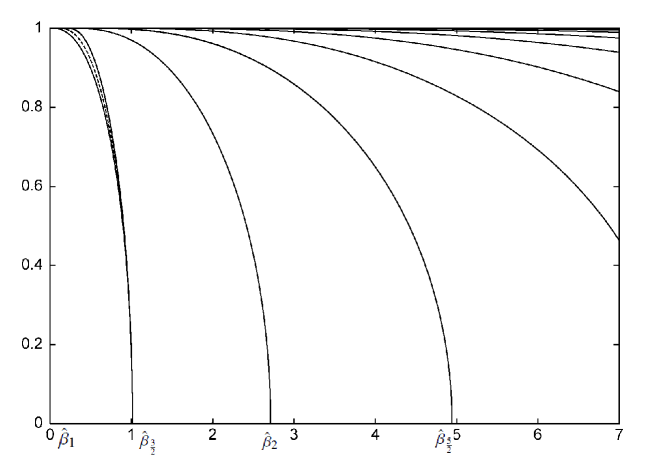
Figure 1: The $1$-degenerate and $-1$-degenerate curves of Euler elliptic relative equilibria of the planar three-body problem in the $(\beta,e)$ rectangle $[0,7]\times[0,1)$.

The concept of “$M\approx N$” for two symplectic matrices $M$ and $N$, i.e., $N\in\Omega^{0}(M)$, was first introduced in [14] of 1999, which can be found in the Definition 5.2 of the Appendix 5.2 in this paper following Definition 1.8.5 of [16]. This notion is broader than the symplectic similarity in general as pointed out on p.38 of [16].

For the normal forms of ${\gamma}_{{\beta},e}(2\pi)$, we have the following theorem.

Theorem 1.5

For the normal forms of ${\gamma}_{{\beta},e}(2\pi)$ when ${\beta}\geq 0,0\leq e<1$, for $n\in{\bf N}$, we have the following results:

(i) If ${\beta}=0$, we have $i_{1}({\gamma}_{0,e}(2\pi))=0$, $\nu_{1}({\gamma}_{0,e}(2\pi))=3$, $i_{-1}({\gamma}_{0,e}(2\pi))=2$, $\nu_{-1}({\gamma}_{0,e}(2\pi))=0$ and ${\gamma}_{0,e}(2\pi)\approx I_{2}\diamond N_{1}(1,1)$;

(ii) If $0<{\beta}<{\beta}_{1}(-1,e)$, we have $i_{1}({\gamma}_{{\beta},e}(2\pi))=3$, $\nu_{1}({\gamma}_{{\beta},e}(2\pi))=0$, $i_{-1}({\gamma}_{{\beta},e}(2\pi))=2$, $\nu_{-1}({\gamma}_{{\beta},e}(2\pi))=0$ and ${\gamma}_{{\beta},e}(2\pi)\approx R(\theta)\diamond D(2)$ for some $\theta\in(0,\pi)$;

(iii) If ${\beta}={\beta}_{1}(-1,e)={\beta}_{2}(-1,e)$, we have $i_{1}({\gamma}_{{\beta},e}(2\pi))=3$, $\nu_{1}({\gamma}_{{\beta},e}(2\pi))=0$, $i_{-1}({\gamma}_{{\beta},e}(2\pi))=2$, $\nu_{-1}({\gamma}_{{\beta},e}(2\pi))=2$ and ${\gamma}_{{\beta},e}(2\pi)\approx-I_{2}\diamond D(2)$;

(iv) If ${\beta}_{1}(-1,e)\neq{\beta}_{2}(-1,e)$ and ${\beta}={\beta}_{1}(-1,e)$, we have $i_{1}({\gamma}_{{\beta},e}(2\pi))=3$, $\nu_{1}({\gamma}_{{\beta},e}(2\pi))=0$, $i_{-1}({\gamma}_{{\beta},e}(2\pi))=2$, $\nu_{-1}({\gamma}_{{\beta},e}(2\pi))=1$ and ${\gamma}_{{\beta},e}(2\pi)\approx N_{1}(-1,-1)\diamond D(2)$;

(v) If ${\beta}_{1}(-1,e)\neq{\beta}_{2}(-1,e)$ and ${\beta}_{1}(-1,e)<{\beta}<{\beta}_{2}(-1,e)$, we have $i_{1}({\gamma}_{{\beta},e}(2\pi))=3$, $\nu_{1}({\gamma}_{{\beta},e}(2\pi))=0$, $i_{-1}({\gamma}_{{\beta},e}(2\pi))=3$, $\nu_{-1}({\gamma}_{{\beta},e}(2\pi))=0$ and ${\gamma}_{{\beta},e}(2\pi)\approx D(-2)\diamond D(2)$;

(vi) If ${\beta}_{1}(-1,e)\neq{\beta}_{2}(-1,e)$ and ${\beta}={\beta}_{2}(-1,e)$, we have $i_{1}({\gamma}_{{\beta},e}(2\pi))=3$, $\nu_{1}({\gamma}_{{\beta},e}(2\pi))=0$, $i_{-1}({\gamma}_{{\beta},e}(2\pi))=3$, $\nu_{-1}({\gamma}_{{\beta},e}(2\pi))=1$ and ${\gamma}_{{\beta},e}(2\pi)\approx N_{1}(-1,1)\diamond D(2)$;

(vii) If ${\beta}_{2}(-1,e)<{\beta}<{\beta}_{1}(1,e)$, we have $i_{1}({\gamma}_{{\beta},e}(2\pi))=3$, $\nu_{1}({\gamma}_{{\beta},e}(2\pi))=0$, $i_{-1}({\gamma}_{{\beta},e}(2\pi))=4$, $\nu_{-1}({\gamma}_{{\beta},e}(2\pi))=0$ and ${\gamma}_{{\beta},e}(2\pi)\approx R(\theta)\diamond D(2)$ for some $\theta\in(\pi,2\pi)$;

(viii) If ${\beta}={\beta}_{2n-1}(1,e)(={\beta}_{2n}(1,e))$, we have $i_{1}({\gamma}_{{\beta},e}(2\pi))=2n+1$, $\nu_{1}({\gamma}_{{\beta},e}(2\pi))=2$, $i_{-1}({\gamma}_{{\beta},e}(2\pi))=2n+2$, $\nu_{-1}({\gamma}_{{\beta},e}(2\pi))=0$ and ${\gamma}_{{\beta},e}(2\pi)\approx I_{2}\diamond D(2)$;

(ix) If ${\beta}_{2n}(1,e)<{\beta}<{\beta}_{2n+1}(-1,e)$, we have $i_{1}({\gamma}_{{\beta},e}(2\pi))=2n+3$, $\nu_{1}({\gamma}_{{\beta},e}(2\pi))=0$, $i_{-1}({\gamma}_{{\beta},e}(2\pi))=2n+2$, $\nu_{-1}({\gamma}_{{\beta},e}(2\pi))=0$ and ${\gamma}_{{\beta},e}(2\pi)\approx R(\theta)\diamond D(2)$ for some $\theta\in(0,\pi)$;

(x) If ${\beta}={\beta}_{2n+1}(-1,e)={\beta}_{2n+2}(-1,e)$, we have $i_{1}({\gamma}_{{\beta},e}(2\pi))=2n+3$, $\nu_{1}({\gamma}_{{\beta},e}(2\pi))=0$, $i_{-1}({\gamma}_{{\beta},e}(2\pi))=2n+2$, $\nu_{-1}({\gamma}_{{\beta},e}(2\pi))=2$ and ${\gamma}_{{\beta},e}(2\pi)\approx-I_{2}\diamond D(2)$;

(xi) If ${\beta}_{2n+1}(-1,e)\neq{\beta}_{2n+2}(-1,e)$ and ${\beta}={\beta}_{2n+1}(-1,e)$, we have $i_{1}({\gamma}_{{\beta},e}(2\pi))=2n+3$, $\nu_{1}({\gamma}_{{\beta},e}(2\pi))=0$, $i_{-1}({\gamma}_{{\beta},e}(2\pi))=2n+2$, $\nu_{-1}({\gamma}_{{\beta},e}(2\pi))=1$ and ${\gamma}_{{\beta},e}(2\pi)\approx N_{1}(-1,-1)\diamond D(2)$;

(xii) If ${\beta}_{2n+1}(-1,e)\neq{\beta}_{2n+2}(-1,e)$ and ${\beta}_{2n+1}(-1,e)<{\beta}<{\beta}_{2n+2}(-1,e)$, we have $i_{1}({\gamma}_{{\beta},e}(2\pi))=2n+3$, $\nu_{1}({\gamma}_{{\beta},e}(2\pi))=0$, $i_{-1}({\gamma}_{{\beta},e}(2\pi))=2n+3$, $\nu_{-1}({\gamma}_{{\beta},e}(2\pi))=0$ and ${\gamma}_{{\beta},e}(2\pi)\approx D(-2)\diamond D(2)$;

(xiii) If ${\beta}_{2n+1}(-1,e)\neq{\beta}_{2n+2}(-1,e)$ and ${\beta}={\beta}_{2n+2}(-1,e)$, we have $i_{1}({\gamma}_{{\beta},e}(2\pi))=2n+3$, $\nu_{1}({\gamma}_{{\beta},e}(2\pi))=0$, $i_{-1}({\gamma}_{{\beta},e}(2\pi))=2n+3$, $\nu_{-1}({\gamma}_{{\beta},e}(2\pi))=1$ and ${\gamma}_{{\beta},e}(2\pi)\approx N_{1}(-1,1)\diamond D(2)$;

(xiv) If ${\beta}_{2n+2}(-1,e)<{\beta}<{\beta}_{2n+1}(1,e)$, we have $i_{1}({\gamma}_{{\beta},e}(2\pi))=2n+3$, $\nu_{1}({\gamma}_{{\beta},e}(2\pi))=0$, $i_{-1}({\gamma}_{{\beta},e}(2\pi))=2n+4$, $\nu_{-1}({\gamma}_{{\beta},e}(2\pi))=0$ and ${\gamma}_{{\beta},e}(2\pi)\approx R(\theta)\diamond D(2)$ for some $\theta\in(\pi,2\pi)$.

In the proof of these theorems, motivated by the techniques of [5], we study properties of the symplectic path ${\gamma}_{{\beta},e}$ in ${\rm Sp}(4)$ and the second order differential operators $A({\beta},e)$ corresponding to ${\gamma}_{{\beta},e}$. To get the information on the indices of ${\gamma}_{{\beta},e}$ for $({\beta},e)\in{\Theta}$, one of the main ingredients of the proof is the non-decreasing property of ${\omega}$-index proved in Lemma 4.2 and Corollary 4.3 below for all ${\omega}\in{\bf U}$.

The rest of this paper is focused on the proof of Theorems 1.1, 1.3 and 1.5. For Theorem 1.1, the index properties in (i)-(iii) are established in Section 3; the non-decreasing property (iv) is proved in Corollary 4.3; the property (v) is proved in Theorem 4.11; the estimate (vi) is proved in Proposition 4.4; and the non-degenerate property (vii) is proved in Theorem 4.6. Theorem 1.5 is proved in the Subsection 4.3. For Theorem 1.3, (i) on the $1$-degenerate curves ${\Gamma}_{n}$ is proved in Subsection 4.3 and Subsection 4.4; (ii) on the $-1$-degenerate curves $\Xi_{n}$ is proved in the Subsection 4.4; and (iii) is prove in the Subsection 4.3.

2 Preliminaries

In the subsection 5.2 of the Appendix, we give a brief review on the Maslov-type ${\omega}$-index theory for ${\omega}$ in the unit circle of the complex plane following [16]. In the following, we use notations introduced there.

2.1 The essential part of the fundamental solution of the elliptic Euler orbit

In [22] (cf. p.275), Meyer and Schmidt gave the essential part of the fundamental solution of the elliptic Lagrangian orbit. Their method is explained in [17] too. Our study on elliptic Euler solutions is based upon their method.

Suppose the three particles are all on the $x$-axis, $q_{1}=0$, $q_{2}=(x\alpha,0)^{T}$ and $q_{3}=((1+x)\alpha,0)^{T}$ for $\alpha=|q_{2}-q_{3}|>0$, $x\alpha=|q_{1}-q_{2}|$ and some $x>0$. When $q_{1}$, $q_{2}$ and $q_{3}$ form a collinear central configurations, $x$ must satisfy Euler’s quintic equation as in p.148 of [2], p.276 of [26] and p.29 of [17]:

$$(m_{3}+m_{2})x^{5}+(3m_{3}+2m_{2})x^{4}+(3m_{3}+m_{2})x^{3}-(3m_{1}+m_{2})x^{2}-(3m_{1}+2m_{2})x-(m_{1}+m_{2})=0.$$ (2.1)

Moreover, by Descartes’ rule of signs for polynomials (cf. p.300 of [10]), polynomial (2.1) has only one positive solution $x$.

Without lose of generality, we normalize the three masses by

$$m_{1}+m_{2}+m_{3}=1.$$ (2.2)

Then the center of mass of the three particles is

$$q_{0}=m_{1}q_{1}+m_{2}q_{2}+m_{3}q_{3}=([m_{2}x+m_{3}(1+x)]\alpha,0)^{T}=([m_{3}+(1-m_{1})x]\alpha,0)^{T},$$

where we used (2.2) in the last equality.

For $i=1,2,3$, let $a_{i}=q_{i}-q_{0}$, and denote by $a_{ix}$ and $a_{iy}$ the $x$ and $y$-coordinates of $a_{i}$ respectively. Then we have

$$a_{1x}=-[m_{3}+(1-m_{1})x]\alpha,\quad a_{2x}=(-m_{3}+m_{1}x)\alpha,\quad a_{3x}=[(1-m_{3})+m_{1}x]\alpha$$ (2.3)

and

$$a_{iy}=0,\quad\quad{\rm for}\;i=1,2,3.$$ (2.4)

Scaling $\alpha$ by setting $\sum_{i=1}^{3}m_{i}|a_{i}|^{2}=1$, we obtain

$$\alpha^{2} = \frac{\alpha^{2}}{\sum_{i=1}^{3}m_{i}|a_{i}|^{2}}=\frac{1}{m_{1}[-m_{3}-(1-m_{1})x]^{2}+m_{2}[-m_{3}+m_{1}x]^{2}+m_{3}[1-m_{3}+m_{1}x]^{2}}$$ (2.5)

$$= \frac{1}{m_{1}(1-m_{1})x^{2}+2m_{1}m_{3}x+m_{3}(1-m_{3})}.$$

Now as in p.263 of [22], Section 11.2 of [17], we define

$$P=\left(\matrix{p_{1}\cr p_{2}\cr p_{3}}\right),\quad Q=\left(\matrix{q_{1}\cr q_{2}\cr q_{3}}\right),\quad Y=\left(\matrix{G\cr Z\cr W}\right),\quad X=\left(\matrix{g\cr z\cr w}\right),$$ (2.6)

where $p_{i}$, $q_{i}$, $i=1,2,3$ and $G$, $Z$, $W$, $g$, $z$, $w$ are all column vectors in ${\bf R}^{2}$. We make the symplectic coordinate change

$$P=A^{-T}Y,\quad Q=AX,$$ (2.7)

where the matrix $A$ is constructed as in the proof of Proposition 2.1 in [22]. Concretely, the matrix $A\in{\bf GL}({\bf R}^{6})$ is given by

$$A=\left(\matrix{I\quad A_{1}\quad B_{1}\cr I\quad A_{2}\quad B_{2}\cr I\quad A_{3}\quad B_{3}}\right),$$ (2.8)

where by (2.3)-(2.4), each $A_{i}$ is a $2\times 2$ matrix given by

$$A_{i}=(a_{i},Ja_{i})=\left(\matrix{a_{ix}\quad 0\cr 0\quad a_{ix}}\right)=a_{ix}I.$$ (2.9)

with $J=\left(\matrix{0&-1\cr 1&0}\right)$.

To fulfill $A^{T}MA=I$ (cf. (13) in p.263 of [22]), we must have

$$B_{1} = \rho_{1}(A_{3}-A_{2})^{T}=\rho_{1}(a_{3x}-a_{2x})I=\rho_{1}\alpha I,$$

$$B_{2} = \rho_{2}(A_{1}-A_{3})^{T}=\rho_{2}(a_{1x}-a_{3x})I=-\rho_{2}(1+x)\alpha I,$$

$$B_{3} = \rho_{3}(A_{2}-A_{1})^{T}=\rho_{3}(a_{2x}-a_{1x})I=\rho_{3}x\alpha I,$$

where

$$\rho_{i}=\frac{\sqrt{m_{1}m_{2}m_{3}}}{m_{i}},\quad\forall 1\leq i\leq 3.$$ (2.10)

Denote by

$$b_{1}=\rho_{1}\alpha,\quad b_{2}=-\rho_{2}(1+x)\alpha,\quad b_{3}=\rho_{3}x\alpha.$$ (2.11)

Then we simply have

$$B_{i}=b_{i}I,\quad\forall 1\leq i\leq 3.$$ (2.12)

Under the coordinate change (2.7), we get the kinetic energy

$$K=\frac{1}{2}(|G|^{2}+|Z|^{2}+|W|^{2}),$$ (2.13)

and the potential function

$$U(z,w)=\sum_{1\leq i<j\leq 3}U_{ij}(z,w),\quad U_{ij}(z,w)=\frac{m_{i}m_{j}}{d_{ij}(z,w)},$$ (2.14)

with

$$d_{ij}(z,w)=|(A_{i}-A_{j})z+(B_{i}-B_{j})w|=|(a_{ix}-a_{jx})z+(b_{i}-b_{j})w|,$$ (2.15)

where we used (2.9) and (2.12).

Let $\theta$ be the true anomaly. In [22], Meyer and Schmidt introduced their celebrated central configuration coordinates, which greatly simplified the corresponding systems. Then under the same steps of symplectic transformation in the proof of Lemma 3.1 in [22], the resulting Hamiltonian function of the 3-body problem is given by

$$H(\theta,\bar{Z},\bar{W},\bar{z},\bar{w})=\frac{1}{2}(|\bar{Z}|^{2}+|\bar{W}|^{2})+(\bar{z}\cdot J\bar{Z}+\bar{w}\cdot J\bar{W})+\frac{p-r(\theta)}{2p}(|\bar{z}|^{2}+|\bar{w}|^{2})-\frac{r(\theta)}{\sigma}U(\bar{z},\bar{w}),$$ (2.16)

where

$$r(\theta)=\frac{p}{1+e\cos\theta},$$ (2.17)

and

$$\mu=\sum_{1\leq i<j\leq 3}\frac{m_{i}m_{j}}{|a_{i}-a_{j}|}=\frac{1}{\alpha}\left(\frac{m_{1}m_{2}}{x}+m_{2}m_{3}+\frac{m_{3}m_{1}}{1+x}\right),\quad\sigma=(\mu p)^{1/4}.$$ (2.18)

Note that here as pointed out in Section 11 of [17], the original constant ${\sigma}=\mu p$ in the line 9 on p.273 of [22] is not correct and should be corrected to ${\sigma}=(\mu p)^{1/4}$. Because this constant and the related corrections in this derivation are crucial in the later computations of the linear stability, we refer readers to Section 2 of [30] for the complete details of derivations of (2.16)-(2.18).

Indeed, $H$ given by (2.16) is essentially the Hamiltonian of the system in the pulsating frame, in which $\theta$ is the new independent variable, and $p=a(1-e^{2})$ with $a$ and $e$ being the semi-major axis and the eccentricity of $z(t)$ respectively.

We now derived the linearized Hamiltonian system at the Euler elliptic solutions.

Proposition 2.1

Using notations in (2.6), elliptic Euler solution $(P(t),Q(t))^{T}$ of the system (1.2) with

$$Q(t)=(r(t)R(\theta(t))a_{1},r(t)R(\theta(t))a_{2},r(t)R(\theta(t))a_{3})^{T},\quad P(t)=M\dot{Q}(t)$$ (2.19)

in time $t$ with the matrix $M=diag(m_{1},m_{1},m_{2},m_{2},m_{3},m_{3})$, is transformed to the new solution $(Y(\theta),X(\theta))^{T}$ in the variable true anomaly $\theta$ with $G=g=0$ with respect to the original Hamiltonian function $H$ of (2.16), which is given by

$$Y(\theta)=\left(\matrix{\bar{Z}(\theta)\cr\bar{W}(\theta)}\right)=\left(\matrix{0\cr\sigma\cr 0\cr 0}\right),\quad X(\theta)=\left(\matrix{\bar{z}(\theta)\cr\bar{w}(\theta)}\right)=\left(\matrix{\sigma\cr 0\cr 0\cr 0}\right).$$ (2.20)

Moreover, the linearized Hamiltonian system at the elliptic Euler solution ${\xi}_{0}\equiv(Y(\theta),X(\theta))^{T}=$
$(0,\sigma,0,0,\sigma,0,0,0)^{T}\in{\bf R}^{8}$ depending on the true anomaly $\theta$ with respect to the Hamiltonian function $H$ of (2.16) is given by

$$\dot{\zeta}(\theta)=JB(\theta)\zeta(\theta),$$ (2.21)

with

$$B(\theta)=H^{\prime\prime}(\theta,\bar{Z},\bar{W},\bar{z},\bar{w})|_{\bar{\xi}=\xi_{0}}=\left(\matrix{I&O&-J&O\cr O&I&O&-J\cr J&O&H_{\bar{z}\bar{z}}(\theta,\xi_{0})&O\cr O&J&O&H_{\bar{w}\bar{w}}(\theta,\xi_{0})}\right),$$ (2.22)

and

$$H_{\bar{z}\bar{z}}(\theta,\xi_{0})=\left(\matrix{-\frac{2-e\cos\theta}{1+e\cos\theta}&0\cr 0&1}\right),\quad H_{\bar{w}\bar{w}}(\theta,\xi_{0})=\left(\matrix{-\frac{2\delta-e\cos\theta}{1+e\cos\theta}&0\cr 0&\frac{\delta+e\cos\theta}{1+e\cos\theta}}\right),$$ (2.23)

where

$$\delta=\frac{1}{\mu}\sum_{1\leq i<j\leq 3}\frac{m_{i}m_{j}(b_{i}-b_{j})^{2}}{|a_{ix}-a_{jx}|^{3}}=\frac{\sum_{1\leq i<j\leq 3}\frac{m_{i}m_{j}(b_{i}-b_{j})^{2}}{|a_{ix}-a_{jx}|^{3}}}{\sum_{1\leq i<j\leq 3}\frac{m_{i}m_{j}}{|a_{ix}-a_{jx}|}},$$ (2.24)

and $H^{\prime\prime}$ is the Hession Matrix of $H$ with respect to its variable $\bar{Z}$, $\bar{W}$, $\bar{z}$ and $\bar{w}$. The corresponding quadratic Hamiltonian function is given by

$$H_{2}(\theta,\bar{Z},\bar{W},\bar{z},\bar{w}) = \frac{1}{2}|\bar{Z}|^{2}+\bar{z}\cdot J\bar{Z}+\frac{1}{2}H_{\bar{z}\bar{z}}(\theta,\xi_{0})|\bar{z}|^{2}$$ (2.25)

$$+\frac{1}{2}|\bar{W}|^{2}+\bar{w}\cdot J\bar{W}+\frac{1}{2}H_{\bar{w}\bar{w}}(\theta,\xi_{0})|\bar{w}|^{2}.$$

Proof. The proof is similar to those of Proposition 11.11 and Proposition 11.13 of [17]. We just need to compute $H_{\bar{z}\bar{z}}(\theta,\xi_{0})$, $H_{\bar{z}\bar{w}}(\theta,\xi_{0})$ and $H_{\bar{w}\bar{w}}(\theta,\xi_{0})$.

For simplicity, we omit all the upper bars on the variables of $H$ in (2.16) in this proof. By (2.16), we have

$$H_{z} = JZ+\frac{p-r}{p}z-\frac{r}{\sigma}U_{z}(z,w),$$

$$H_{w} = JW+\frac{p-r}{p}w-\frac{r}{\sigma}U_{w}(z,w),$$

and

$$\left\{\begin{array}[]{l}H_{zz}=\frac{p-r}{p}I-\frac{r}{\sigma}U_{zz}(z,w),\\ H_{zw}=H_{wz}=-\frac{r}{\sigma}U_{zw}(z,w),\\ H_{ww}=\frac{p-r}{p}I-\frac{r}{\sigma}U_{ww}(z,w),\end{array}\right.$$ (2.26)

where we write $H_{z}$ and $H_{zw}$ etc to denote the derivative of $H$ with respect to $z$, and the second derivative of $H$ with respect to $z$ and then $w$ respectively. Note that all the items above are $2\times 2$ matrices.

For $U_{ij}$ defined in (2.14) with $1\leq i<j\leq 3$, we have

$$\frac{\partial U_{ij}}{\partial z}(z,w) = -\frac{m_{i}m_{j}(a_{ix}-a_{jx})}{|(a_{ix}-a_{jx})z+(b_{i}-b_{j})w|^{3}}\left[(a_{ix}-a_{jx})z+(b_{i}-b_{j})w\right],$$

$$\frac{\partial U_{ij}}{\partial w}(z,w) = -\frac{m_{i}m_{j}(b_{i}-b_{j})}{|(a_{ix}-a_{jx})z+(b_{i}-b_{j})w|^{3}}\left[(a_{ix}-a_{jx})z+(b_{i}-b_{j})w\right],$$

and

$$\frac{\partial^{2}U_{ij}}{\partial z^{2}}(z,w)=-\frac{m_{i}m_{j}(a_{ix}-a_{jx})^{2}}{|(a_{ix}-a_{jx})z+(b_{i}-b_{j})w|^{3}}I$$

$$\quad+3\frac{m_{i}m_{j}(a_{ix}-a_{jx})^{2}}{|(a_{ix}-a_{jx})z+(b_{i}-b_{j})w|^{5}}\left[(a_{ix}-a_{jx})z+(b_{i}-b_{j})w\right]\left[(a_{ix}-a_{jx})z+(b_{i}-b_{j})w\right]^{T},$$

$$\frac{\partial^{2}U_{ij}}{\partial z\partial w}(z,w)=-\frac{m_{i}m_{j}(a_{ix}-a_{jx})(b_{i}-b_{j})}{|(a_{ix}-a_{jx})z+(b_{i}-b_{j})w|^{3}}I$$

$$\quad+3\frac{m_{i}m_{j}(a_{ix}-a_{jx})(b_{i}-b_{j})}{|(a_{ix}-a_{jx})z+(b_{i}-b_{j})w|^{5}}\left[(a_{ix}-a_{jx})z+(b_{i}-b_{j})w\right]\left[(a_{ix}-a_{jx})z+(b_{i}-b_{j})w\right]^{T},$$

$$\frac{\partial^{2}U_{ij}}{\partial w^{2}}(z,w)=-\frac{m_{i}m_{j}(b_{i}-b_{j})^{2}}{|(a_{ix}-a_{jx})z+(b_{i}-b_{j})w|^{3}}I$$

$$\quad+3\frac{m_{i}m_{j}(b_{i}-b_{j})^{2}}{|(a_{ix}-a_{jx})z+(b_{i}-b_{j})w|^{5}}\left[(a_{ix}-a_{jx})z+(b_{i}-b_{j})w\right]\left[(a_{ix}-a_{jx})z+(b_{i}-b_{j})w\right]^{T}.$$

Let

$$K=\left(\matrix{2&0\cr 0&-1}\right),\quad K_{1}=\left(\matrix{1&0\cr 0&0}\right).$$

Now evaluating these functions at the solution $\bar{\xi}_{0}=(0,\sigma,0,0,\sigma,0,0,0)^{T}\in{\bf R}^{8}$ with $z=(\sigma,0)^{T},w=(0,0)^{T}$, and summing them up, we obtain

$$\frac{\partial^{2}U}{\partial z^{2}}\left|{}_{\xi_{0}}\right. = \sum_{1\leq i<j\leq 3}\frac{\partial^{2}U_{ij}}{\partial z^{2}}\left|{}_{\xi_{0}}\right.$$ (2.27)

$$= \sum_{1\leq i<j\leq 3}\left(-\frac{m_{i}m_{j}(a_{ix}-a_{jx})^{2}}{|(a_{ix}-a_{jx})\sigma|^{3}}I+3\frac{m_{i}m_{j}(a_{ix}-a_{jx})^{2}}{|(a_{ix}-a_{jx})\sigma|^{5}}(a_{ix}-a_{jx})^{2}\sigma^{2}K_{1}\right)$$

$$= \frac{1}{\sigma^{3}}\left(\sum_{1\leq i<j\leq 3}\frac{m_{i}m_{j}}{|a_{ix}-a_{jx}|}\right)K$$

$$= \frac{\mu}{\sigma^{3}}K,$$

$$\frac{\partial^{2}U}{\partial w^{2}}\left|{}_{\xi_{0}}\right. = \sum_{1\leq i<j\leq 3}\frac{\partial^{2}U_{ij}}{\partial w^{2}}\left|{}_{\xi_{0}}\right.$$ (2.28)

$$= \sum_{1\leq i<j\leq 3}\left(-\frac{m_{i}m_{j}(b_{i}-b_{j})^{2}}{|(a_{ix}-a_{jx})\sigma|^{3}}I+3\frac{m_{i}m_{j}(b_{i}-b_{j})^{2}}{|(a_{ix}-a_{jx})\sigma|^{5}}(a_{ix}-a_{jx})^{2}\sigma^{2}K_{1}\right)$$

$$= \frac{1}{\sigma^{3}}\left(\sum_{1\leq i<j\leq 3}\frac{m_{i}m_{j}(b_{i}-b_{j})^{2}}{|a_{ix}-a_{jx}|^{3}}\right)K$$

$$= \frac{\delta\mu}{\sigma^{3}}K,$$

where in the third equality of the first formula, we used (2.18), and in the last equality of the second formula, we use the definition (2.24). Similarly, we have

$$\frac{\partial^{2}U}{\partial z\partial w}\left|{}_{\xi_{0}}\right. = \sum_{1\leq i<j\leq 3}\frac{\partial^{2}U_{ij}}{\partial z\partial w}\left|{}_{\xi_{0}}\right.$$ (2.29)

$$= \sum_{1\leq i<j\leq 3}\left(-\frac{m_{i}m_{j}(a_{ix}-a_{jx})(b_{i}-b_{j})}{|(a_{ix}-a_{jx})\sigma|^{3}}I+3\frac{m_{i}m_{j}(a_{ix}-a_{jx})(b_{i}-b_{j})}{|(a_{ix}-a_{jx})\sigma|^{5}}(a_{ix}-a_{jx})^{2}\sigma^{2}K_{1}\right)$$

$$= \left(\sum_{1\leq i<j\leq 3}\frac{m_{i}m_{j}(b_{i}-b_{j})\cdot sign(a_{ix}-a_{jx})}{|(a_{ix}-a_{jx})|^{2}}\right)\frac{K}{\sigma^{3}}$$

$$= \left(\frac{m_{1}m_{2}\sqrt{m_{1}m_{2}m_{3}}\alpha(\frac{1}{m_{1}}+\frac{1+x}{m_{2}})\cdot sign(-x\alpha)}{(-x\alpha)^{2}}+\frac{m_{2}m_{3}[-\sqrt{m_{1}m_{2}m_{3}}\alpha(\frac{1+x}{m_{2}}+\frac{x}{m_{3}})]\cdot sign(-\alpha)}{(-\alpha)^{2}}\right.$$

$$+\left.\frac{m_{3}m_{1}\sqrt{m_{1}m_{2}m_{3}}\alpha(\frac{x}{m_{3}}-\frac{1}{m_{1}})\cdot sign((1+x)\alpha)}{((1+x)\alpha)^{2}}\right)\frac{K}{\sigma^{3}}$$

$$= \frac{\sqrt{m_{1}m_{2}m_{3}}}{\alpha}\left(-\frac{m_{2}+m_{1}+m_{1}x}{x^{2}}+(m_{2}+m_{3})x+m_{3}+\frac{m_{1}x-m_{3}}{(1+x)^{2}}\right)\frac{K}{\sigma^{3}}$$

$$= O,$$

where in the third equality, we used (2.3) and (2.11), and in the last equality, we used

$$-\frac{m_{2}+m_{1}x}{x^{2}}+(m_{2}+m_{3})x+m_{3}+\frac{m_{1}x-m_{3}}{(1+x)^{2}}$$

$$=\frac{(m_{2}+m_{3})x^{5}+(2m_{2}+3m_{3})x^{4}+(m_{2}+3m_{3})x^{3}-(3m_{1}+m_{2})x^{2}-(3m_{1}+2m_{2})x-(m_{1}+m_{2})}{x^{2}(1+x)^{2}}$$

$$=0.$$ (2.30)

By (2.27), (2.28), (2.29) and (2.26), we have

$$H_{zz}|_{\xi_{0}} = \frac{p-r}{p}I-\frac{r\mu}{\sigma^{4}}K=I-\frac{r}{p}I-\frac{r\mu}{p\mu}K=I-\frac{r}{p}(I+K)=\left(\matrix{-\frac{2-e\cos\theta}{1+e\cos\theta}&0\cr 0&1}\right),$$

$$H_{zw}|_{\xi_{0}} = -\frac{r}{\sigma}\frac{\partial^{2}U}{\partial z\partial w}|_{\xi_{0}}=O,$$

$$H_{ww}|_{\xi_{0}} = \frac{p-r}{p}I-\frac{r\delta\mu}{\sigma^{4}}K=I-\frac{r}{p}I-\frac{r\delta\mu}{p\mu}K=I-\frac{r}{p}(I+\delta K)=\left(\matrix{-\frac{2\delta-e\cos\theta}{1+e\cos\theta}&0\cr 0&\frac{\delta+e\cos\theta}{1+e\cos\theta}}\right).$$

Thus the proof is complete. 

We now want to obtain a simpler representation of $\delta$ of (2.24). Plugging (2.3) and (2.11) into (2.24), we have

$$\delta = \frac{\frac{m_{1}m_{2}}{x^{3}}(\rho_{1}+\rho_{2}(1+x))^{2}+m_{2}m_{3}(\rho_{2}(1+x)+\rho_{3}x)^{2}+\frac{m_{3}m_{1}}{(1+x)^{3}}(\rho_{3}x-\rho_{1})^{2}}{\frac{m_{1}m_{2}}{x}+m_{2}m_{3}+\frac{m_{3}m_{1}}{1+x}}$$ (2.31)

$$= \frac{m_{3}(1+x)^{3}(m_{2}+m_{1}+m_{1}x)^{2}+m_{1}x^{3}(1+x)^{3}(m_{3}+m_{3}x+m_{2}x)^{2}+m_{2}x^{3}(m_{1}x-m_{3})^{2}}{x^{2}(1+x)^{2}[m_{2}m_{3}x^{2}+(m_{1}m_{2}+m_{2}m_{3}+m_{3}m_{1})x+m_{1}m_{2}]}$$

$$= 1+\frac{m_{1}(3x^{2}+3x+1)+m_{3}x^{2}(x^{2}+3x+3)}{x^{2}+m_{2}[(x+1)^{2}(x^{2}+1)-x^{2}]},$$

where $\rho_{i}$ are given by (2.10), and the last equality holds by Lemma 5.1 in the Appendix. Note that $m_{3}=1-m_{1}-m_{2}$, the second term in the last equality of (2.31) is also defined in (18) of [18] (p. 317) and we use the same symbol $\beta$ of (1.4) to denote it, and $\delta=\beta+1$. Then writing $H_{\bar{w}\bar{w}}(\theta,\bar{\xi}_{0})$ in terms of $\beta$ yields

$$H_{\bar{w}\bar{w}}(\theta,\xi_{0})=\left(\matrix{-\frac{2\beta+2-e\cos\theta}{1+e\cos\theta}&0\cr 0&\frac{\beta+1+e\cos\theta}{1+e\cos\theta}}\right).$$ (2.32)

Moreover, by the proof of Lemma 2 of [18], we know that the full range of $\beta$ is $[0,7]$ when $m_{1},m_{2},m_{3}$ take all their possible values. Thus we have

Proposition 2.2

The full range of the pair $(\beta,e)$ of the Euler elliptic orbit is the rectangle $[0,7]\times[0,1)$.

By Proposition 2.1 , the essential part ${\gamma}={\gamma}_{{\beta},e}(t)$ of the fundamental solution of the Euler orbit satisfies

$$\dot{\gamma}(t) = JB(t)\gamma(t),$$ (2.33)

$$\gamma(0) = I_{4},$$ (2.34)

with

$$B(t)=\left(\matrix{1&0&0&1\cr 0&1&-1&0\cr 0&-1&\frac{-2\beta-2+e\cos(t)}{1+e\cos(t)}&0\cr 1&0&0&\frac{\beta+1+e\cos(t)}{1+e\cos(t)}\cr}\right),$$ (2.35)

where $e$ is the eccentricity, and $t$ is the truly anomaly.

Let

$$J_{2}=\left(\matrix{0&-1\cr 1&0\cr}\right),\qquad K_{{\beta},e}(t)=\left(\matrix{\frac{2\beta+3}{1+e\cos(t)}&0\cr 0&-\frac{\beta}{1+e\cos(t)}\cr}\right),$$ (2.36)

and set

$$L(t,x,\dot{x})=\frac{1}{2}\|\dot{x}\|^{2}+J_{2}x(t)\cdot\dot{x}(t)+\frac{1}{2}K_{{\beta},e}(t)x(t)\cdot x(t),\qquad\quad\forall\;x\in W^{1,2}({\bf R}/2\pi{\bf Z},{\bf R}^{2}),$$ (2.37)

where $a\cdot b$ denotes the inner product in ${\bf R}^{2}$. Obviously the origin in the configuration space is a solution of the corresponding Euler-Lagrange system. By Legendrian transformation, the corresponding Hamiltonian function is

$$H(t,z)=\frac{1}{2}B(t)z\cdot z,\qquad\forall\;z\in{\bf R}^{4}.$$

2.2 A modification on the path ${\gamma}_{{\beta},e}(t)$

In order to transform the Lagrangian system (2.35) to a simpler linear operator corresponding to a second order Hamiltonian system with the same linear stability as ${\gamma}_{{\beta},e}(2\pi)$, using $R(t)$ and $R_{4}(t)={\rm diag}(R(t),R(t))$ as in Section 2.4 of [5], we let

$$\xi_{{\beta},e}(t)=R_{4}(t){\gamma}_{{\beta},e}(t),\qquad\forall\;t\in[0,2\pi],({\beta},e)\in[0,7]\times[0,1).$$ (2.38)

One can show by direct computation that

$$\frac{d}{dt}\xi_{{\beta},e}(t)=J\left(\matrix{I_{2}&0\cr 0&R(t)(I_{2}-K_{{\beta},e}(t))R(t)^{T}\cr}\right)\xi_{{\beta},e}(t).$$ (2.39)

Note that $R_{4}(0)=R_{4}(2\pi)=I_{4}$, so ${\gamma}_{{\beta},e}(2\pi)=\xi_{{\beta},e}(2\pi)$ holds. Then the linear stabilities of the systems (2.34) and (2.39) are determined by the same matrix and thus is precisely the same.

By (2.38) the symplectic paths ${\gamma}_{{\beta},e}$ and $\xi_{{\beta},e}$ are homotopic to each other via the homotopy $h(s,t)=R_{4}(st){\gamma}_{{\beta},e}(t)$ for $(s,t)\in[0,1]\times[0,2\pi]$. Because $R_{4}(s){\gamma}_{{\beta},e}(2\pi)$ for $s\in[0,1]$ is a loop in ${\rm Sp}(4)$ which is homotopic to the constant loop ${\gamma}_{{\beta},e}(2\pi)$, $h(\cdot,2\pi)$ is contractible in ${\rm Sp}(4)$. Therefore by the proof of Lemma 5.2.2 on p.117 of [16], the homotopy between ${\gamma}_{{\beta},e}$ and $\xi_{{\beta},e}$ can be modified to fix the end point ${\gamma}_{{\beta},e}(2\pi)$ for all $s\in[0,1]$. Thus by the homotopy invariance of the Maslov-type index (cf. (i) of Theorem 6.2.7 on p.147 of [16]) we obtain

$$i_{{\omega}}(\xi_{{\beta},e})=i_{{\omega}}({\gamma}_{{\beta},e}),\quad\nu_{{\omega}}(\xi_{{\beta},e})=\nu_{{\omega}}({\gamma}_{{\beta},e}),\qquad\forall\,\omega\in{\bf U},\;({\beta},e)\in[0,7]\times[0,1).$$ (2.40)

Note that the first order linear Hamiltonian system (2.39) corresponds to the following second order linear Hamiltonian system

$$\ddot{x}(t)=-x(t)+R(t)K_{{\beta},e}(t)R(t)^{T}x(t).$$ (2.41)

For $({\beta},e)\in[0,7)\times[0,1)$, the second order differential operator corresponding to (2.41) is given by

$$A({\beta},e) = -\frac{d^{2}}{dt^{2}}I_{2}-I_{2}+R(t)K_{{\beta},e}(t)R(t)^{T}$$ (2.42)

$$= -\frac{d^{2}}{dt^{2}}I_{2}-I_{2}+\frac{1}{2(1+e\cos t)}((3+\beta)I_{2}+3(1+\beta)S(t)),$$

where $S(t)=\left(\matrix{\cos 2t&\sin 2t\cr\sin 2t&-\cos 2t\cr}\right)$, defined on the domain $\overline{D}(\omega,2\pi)$ in (5.28). Then it is self-adjoint and depends on the parameters ${\beta}$ and $e$. By Lemma 5.6, we have for any ${\beta}$ and $e$, the Morse index $\phi_{{\omega}}(A({\beta},e))$ and nullity $\nu_{{\omega}}(A({\beta},e))$ of the operator $A({\beta},e)$ on the domain $\overline{D}(\omega,2\pi)$ satisfy

$$\phi_{{\omega}}(A({\beta},e))=i_{{\omega}}(\xi_{{\beta},e}),\quad\nu_{{\omega}}(A({\beta},e))=\nu_{{\omega}}(\xi_{{\beta},e}),\qquad\forall\,{\omega}\in{\bf U}.$$ (2.43)

In the rest of this paper, we shall use both of the paths ${\gamma}_{{\beta},e}$ and $\xi_{{\beta},e}$ to study the linear stability of ${\gamma}_{{\beta},e}(2\pi)=\xi_{{\beta},e}(2\pi)$. Because of (2.40), in many cases and proofs below, we shall not distinguish these two paths. Hence, if there is no confusion, we will use $i_{\omega}({\beta},e)$ and $\nu_{\omega}({\beta},e)$ to represent $i_{{\omega}}({\gamma}_{{\beta},e})$ and $\nu_{{\omega}}({\gamma}_{{\beta},e})$ respectively.

3 Stability on the boundary of the unbounded rectangle $[0,\infty)\times[0,1)$

We start from the following lemma which will be used in sections 3 and 4. It is a special case of Theorem 8.3.1 on p.188 of [16], the details of whose proof is left to readers there based on the ideas in the proofs of Theorems 8.2.1 and 8.2.2 on pp.184-185 of [16]. For reader’s conveniences, we give a detailed proof of this lemma here.

Lemma 3.1

Let ${\gamma}\in\mathcal{P}_{\tau}(4)$ satisfy

$${\gamma}(\tau)\approx M_{1}{\rm\diamond}M_{2}$$ (3.1)

with $M_{1}$, $M_{2}\in{\rm Sp}(2)$. Then there exist two paths ${\gamma}_{i}\in\mathcal{P}_{\tau}(2)$ with ${\gamma}_{i}(\tau)=M_{i}$ for $i=1,2$ such that we have

$$i_{1}({\gamma})\;=\;i_{1}({\gamma}_{1})+i_{1}({\gamma}_{2})\qquad{\it and}\qquad{\gamma}\;\sim\;{\gamma}_{1}{\rm\diamond}{\gamma}_{2}.$$ (3.2)

Proof. Firstly by Definition 5.2 below of ${\gamma}(\tau)\approx M_{1}{\rm\diamond}M_{2}$ in (3.1), there exists a continuous path $f\in C([0,\tau],{\Omega}({\gamma}(\tau)))$ such that $f(0)={\gamma}(\tau)$ and $f(\tau)=M_{1}{\rm\diamond}M_{2}$. We choose two paths $\xi$ and ${\gamma}_{2}\in\mathcal{P}_{\tau}(2)$ satisfying $\xi(\tau)=M_{1}$ and ${\gamma}_{2}(\tau)=M_{2}$. Then $f\ast{\gamma}(\tau)=M_{1}{\rm\diamond}M_{2}=\xi{\rm\diamond}{\gamma}_{2}(\tau)$. Thus by Lemma 5.2.6 and Definition 5.2.7 on p.120 and Definition 5.4.2 on p.129 of [16], there exists an integer $k\in{\bf Z}$ such that

$$i_{1}(f\ast{\gamma})-(i_{1}(\xi)+i_{1}({\gamma}_{2}))=2k.$$

Let $\phi_{k}(t)=R(2k\pi t/\tau)$ for $t\in[0,\tau]$. Define

$${\gamma}_{1}(t)=\xi\ast\phi_{k}(t),\qquad\forall\;t\in[0,\tau].$$

Then we obtain

$$i_{1}({\gamma}_{1})+i_{1}({\gamma}_{2})=2k+i_{1}(\xi)+i_{1}({\gamma}_{2})=i_{1}(f\ast{\gamma}).$$

Thus by Theorem 6.2.4 on p.146 of [16] and the definition of the path $f$, we obtain

$${\gamma}_{1}{\rm\diamond}{\gamma}_{2}\;\sim\;f\ast{\gamma}\;\sim\;{\gamma},$$

which completes the proof.  

By Proposition 2.2, we know the full range of $({\beta},e)$ is $[0,7]\times[0,1)$. For convenience in the mathematical study, we extend the range of $({\beta},e)$ to $[0,\infty)\times[0,1)$.

Firstly, we need more precise information on indices and stabilities of ${\gamma}_{{\beta}.e}$ at the boundary of the $({\beta},e)$ rectangle $[0,\infty)\times[0,1)$.

3.1 The boundary segment $\{0\}\times[0,1)$

When $\beta=0$, this is the case if $m_{1}=0,\ m_{2}=1,\ m_{3}=0$, and the essential part of the fundamental solution of Euler orbit is also the fundamental solution of the Keplerian orbits. This is just the same case which has been discussed in Section 3.1 of [5]. We just cite the results here:

$$i_{{\omega}}({\gamma}_{0,e})=i_{{\omega}}(\xi_{0,e})=\left\{\begin{array}[]{l}0,\quad{\rm if}\;\;{\omega}=1,\\ 2,\quad{\rm if}\;\;{\omega}\in{\bf U}\setminus\{1\},\end{array}\right.$$ (3.5)

$$\nu_{{\omega}}({\gamma}_{0,e})=\nu_{{\omega}}(\xi_{0,e})=\left\{\begin{array}[]{l}3,\quad{\rm if}\;\;{\omega}=1,\\ 0,\quad{\rm if}\;\;{\omega}\in{\bf U}\setminus\{1\}.\end{array}\right.$$ (3.8)

3.2 The boundary $[0,\infty)\times\{0\}$

In this case $e=0$. It is considered in (A) of Subsection 3.1 of [5] when ${\beta}=0$. Below, we shall first recall the properties of eigenvalues of ${\gamma}_{{\beta},0}(2\pi)$. Then we carry out the computations of normal forms of ${\gamma}_{{\beta},0}(2\pi)$, and $\pm 1$ indices $i_{\pm 1}({\gamma}_{{\beta},0})$ of the path ${\gamma}_{{\beta},0}$ for all ${\beta}\in[0,\infty)$, which are new.

In this case, the essential part of the motion (2.33)-(2.35) becomes an ODE system with constant coefficients:

$$B=B(t)=\left(\matrix{1&0&0&1\cr 0&1&-1&0\cr 0&-1&-2{\beta}-2&0\cr 1&0&0&{\beta}+1\cr}\right).$$ (3.9)

The characteristic polynomial $\det(JB-\lambda I)$ of $JB$ is given by

$$\lambda^{4}+(1-{\beta})\lambda^{2}-{\beta}(2{\beta}+3)=0.$$ (3.10)

Letting ${\alpha}=\lambda^{2}$, the two roots of the quadratic polynomial ${\alpha}^{2}+(1-{\beta}){\alpha}-{\beta}(2{\beta}+3)$ are given by ${\alpha}_{1}=\frac{{\beta}-1+\sqrt{9{\beta}^{2}+10{\beta}+1}}{2}\geq 0$ and ${\alpha}_{2}=\frac{{\beta}-1-\sqrt{9{\beta}^{2}+10{\beta}+1}}{2}<0$. Therefore the four roots of the polynomial (3.10) are given by

$${\alpha}_{1,\pm} = \pm\sqrt{{\alpha}_{1}}=\pm\sqrt{\frac{{\beta}-1+\sqrt{9{\beta}^{2}+10{\beta}+1}}{2}}\in{\bf R},$$ (3.11)

$${\alpha}_{2,\pm} = \pm\sqrt{-1}\sqrt{-{\alpha}_{2}}=\pm\sqrt{-1}\sqrt{\frac{-{\beta}+1+\sqrt{9{\beta}^{2}+10{\beta}+1}}{2}}.$$ (3.12)

Moreover, when ${\beta}\geq 0$, we have

$$\frac{d{\alpha}_{1}}{d{\beta}}=\frac{1}{2}+\frac{9{\beta}+5}{2\sqrt{9{\beta}^{2}+10{\beta}+1}}>0,$$ (3.13)

$$\frac{d{\alpha}_{2}}{d{\beta}}=\frac{1}{2}-\frac{9{\beta}+5}{2\sqrt{9{\beta}^{2}+10{\beta}+1}}<0.$$ (3.14)

(A) Eigenvalues of ${\gamma}_{{\beta},0}(2\pi)$ for ${\beta}\in[0,\infty)$.

When ${\beta}\geq 0$, by (3.11) and (3.12), we get the four characteristic multipliers of the matrix ${\gamma}_{{\beta},0}(2\pi)$

$$\rho_{1,\pm}(\beta)=e^{2\pi{\alpha}_{1,\pm}}=e^{\pm 2\pi\sqrt{{\alpha}_{1}}}\in{\bf R}^{+},$$ (3.15)

$$\rho_{2,\pm}(\beta)=e^{2\pi{\alpha}_{2,\pm}}=e^{\pm 2\pi\sqrt{-1}{\theta}({\beta})},$$ (3.16)

where

$${\theta}({\beta})=\sqrt{\frac{-{\beta}+1+\sqrt{9{\beta}^{2}+10{\beta}+1}}{2}}.$$ (3.17)

By (3.14) and (3.17), we know that ${\theta}({\beta})$ is increasing with respect to ${\beta}$ when ${\beta}\geq 0$.

From (3.17), ${\theta}(0)=1$. Then for any ${\theta}\geq 1$, we denote by ${\beta}_{\theta}\geq 0$ the ${\beta}$ value satisfying ${\theta}({\beta})={\theta}$, and we obtain

$${\theta}=\sqrt{\frac{-{\beta}_{\theta}+1+\sqrt{9{\beta}_{\theta}^{2}+10{\beta}_{\theta}+1}}{2}},$$

and hence

$${\beta}_{\theta}=\frac{{\theta}^{2}-3+\sqrt{9{\theta}^{4}-14{\theta}^{2}+9}}{4},\quad\quad{\theta}\geq 1.$$ (3.18)

Moreover, when ${\theta}\geq 1$, we have

$$\frac{d{\beta}_{\theta}}{d{\theta}}=\frac{2{\theta}+\frac{2{\theta}(9{\theta}^{2}-7)}{\sqrt{9{\theta}^{4}-14{\theta}^{2}+9}}}{4}>0.$$ (3.19)

For later use, we write ${\beta}_{\theta}$ for ${\theta}=n$ and ${\theta}=n+\frac{1}{2}$, $n\in{\bf N}$ as

$$\hat{\beta}_{n}=\frac{n^{2}-3+\sqrt{9n^{4}-14n^{2}+9}}{4},\quad\quad n=1,\;2,\;3...$$ (3.20)

and

$$\hat{\beta}_{n+\frac{1}{2}}=\frac{(n+\frac{1}{2})^{2}-3+\sqrt{9(n+\frac{1}{2})^{4}-14(n+\frac{1}{2})^{2}+9}}{4},\quad\quad n=1,\;2,\;3...$$ (3.21)

where we have used the symbol hat to denote these special values of ${\beta}$. Moreover, from (3.20) we have

$$\hat{\beta}_{n} = \frac{n^{2}-3+\sqrt{9n^{4}-14n^{2}+9}}{4}$$ (3.22)

$$= n^{2}-\frac{3n^{2}+3-\sqrt{9n^{4}-14n^{2}+9}}{4}$$

$$= n^{2}-\frac{32n^{2}}{4(3n^{2}+3+\sqrt{9n^{4}-14n^{2}+9})}$$

$$= n^{2}-\frac{8}{3+\frac{3}{n^{2}}+\sqrt{9-\frac{14}{n^{2}}+\frac{9}{n^{4}}}}$$

$$\approx n^{2}-\frac{4}{3},$$

when $n$ is large enough. By (3.19), we have

$$0=\hat{\beta}_{1}<\hat{\beta}_{\frac{3}{2}}<\hat{\beta}_{2}<\hat{\beta}_{\frac{5}{2}}<...<\hat{\beta}_{n}<\hat{\beta}_{n+\frac{1}{2}}<...$$ (3.23)

Specially, we obtain the following results:

(i) When ${\beta}=\hat{\beta}_{1}=0$, we have ${\sigma}({\gamma}_{0,0}(2\pi))=\{1,1,1,1\}$.

When ${\beta}>0$, by (3.13), (3.14) and (3.15), we have ${\alpha}_{1}>0$, and hence $\rho_{1,\pm}({\beta})=e^{\pm 2\pi\sqrt{{\alpha}_{1}}}\subset{\bf R}\setminus{\bf U}$.

(ii) Let $i\in{\bf N}$. When $\hat{\beta}_{i}<{\beta}<\hat{\beta}_{i+\frac{1}{2}}$, the angle ${\theta}({\beta})$ in (3.17) increases strictly from $i$ to $i+\frac{1}{2}$ as ${\beta}$ increases from $\hat{\beta}_{i}$ to $\hat{\beta}_{i+\frac{1}{2}}$. Therefore $\rho_{2,+}({\beta})=e^{2\pi\sqrt{-1}{\theta}({\beta})}$ runs from $1$ to $-1$ counterclockwise along the upper semi-unit circle in the complex plane ${\bf C}$ as ${\beta}$ increases from $\hat{\beta}_{i}$ to $\hat{\beta}_{i+\frac{1}{2}}$. Correspondingly $\rho_{2,-}({\beta})=e^{-2\pi\sqrt{-1}{\theta}({\beta})}$ runs from $1$ to $-1$ clockwise along the lower semi-unit circle in ${\bf C}$ as ${\beta}$ increases from $\hat{\beta}_{i}$ to $\hat{\beta}_{i+\frac{1}{2}}$. Thus specially we obtain $\rho_{2,\pm}({\beta})\subset{\bf U}\setminus{\bf R}$ for all ${\beta}\in(\hat{\beta}_{i},\hat{\beta}_{i+\frac{1}{2}})$.

(iii) When ${\beta}=\hat{\beta}_{i+\frac{1}{2}}$, we have ${\theta}(\hat{\beta}_{i+\frac{1}{2}})=i+\frac{1}{2}$. Therefore we obtain $\rho_{2,\pm}(\hat{\beta}_{i+\frac{1}{2}})=e^{\pm\sqrt{-1}\pi}=-1$.

(iv) When $\hat{\beta}_{i+\frac{1}{2}}<{\beta}<\hat{\beta}_{i+1}$, the angle ${\theta}({\beta})$ increases strictly from $i+\frac{1}{2}$ to $i+1$ as ${\beta}$ increase from $\hat{\beta}_{i+\frac{1}{2}}$ to $\hat{\beta}_{i+1}$. Thus $\rho_{2,+}({\beta})=e^{2\pi\sqrt{-1}{\theta}({\beta})}$ runs from $-1$ to $1$ counterclockwise along the lower semi-unit circle in ${\bf C}$ as ${\beta}$ increases from $\hat{\beta}_{i+\frac{1}{2}}$ to $\hat{\beta}_{i+1}$. Correspondingly $\rho_{2,-}({\beta})=e^{-2\pi\sqrt{-1}{\theta}({\beta})}$ runs from $-1$ to $1$ clockwise along the upper semi-unit circle in ${\bf C}$ as ${\beta}$ increases from $\hat{\beta}_{i+\frac{1}{2}}$ to $\hat{\beta}_{i+1}$. Thus we obtain $\rho_{2,\pm}({\beta})\subset{\bf U}\setminus{\bf R}$ for all ${\beta}\in(\hat{\beta}_{i+\frac{1}{2}},\hat{\beta}_{i+1})$.

(v) When ${\beta}=\hat{\beta}_{i+1}$, we obtain ${\theta}(\hat{\beta}_{i+1})=i+1$, and then we have double eigenvalues $\rho_{2,\pm}(\hat{\beta}_{i+1})=1$.

(B) Indices $i_{1}({\gamma}_{{\beta},0})$ of ${\gamma}_{{\beta},0}(2\pi)$ for ${\beta}\in[0,\infty)$.

Define

$$f_{0,1}=R(t)\left(\matrix{1\cr 0}\right),\quad f_{0,2}=R(t)\left(\matrix{0\cr 1}\right),$$ (3.24)

and

$$f_{n,1}=R(t)\left(\matrix{\cos nt\cr 0}\right),\quad f_{n,2}=R(t)\left(\matrix{0\cr\cos nt}\right),\quad f_{n,3}=R(t)\left(\matrix{\sin nt\cr 0}\right),\quad f_{n,4}=R(t)\left(\matrix{0\cr\sin nt}\right),$$ (3.25)

for $n\in{\bf N}$. Then $f_{0,1},\;f_{0,2}$ and $f_{n,1},\;f_{n,2}\;f_{n,3},\;f_{n,4}\;n\in{\bf N}$ form an orthogonal basis of $\overline{D}(1,2\pi)$. By (2.42) and $\frac{dR(t)}{dt}=JR(t)$, computing $A({\beta},0)f_{n,1}$ yields

$$A({\beta},0)f_{n,1} = [-\frac{d^{2}}{dt^{2}}I_{2}-I_{2}+R(t)K_{0,e}(t)R(t)^{T}]R(t)\left(\matrix{\cos nt\cr 0}\right)$$ (3.26)

$$= R(t)\left(\matrix{(n^{2}+2{\beta}+3)\cos nt\cr 2n\sin nt}\right)$$

$$= (n^{2}+2{\beta}+3)f_{n,1}+2nf_{n,4}.$$

Similarly, we have

$$\left(\matrix{A({\beta},0)&O\cr O&A({\beta},0)}\right)\left(\matrix{f_{0,1}\cr f_{0,2}}\right) = \left(\matrix{2{\beta}+3&0\cr 0&-{\beta}}\right)\left(\matrix{f_{0,1}\cr f_{0,2}}\right),$$ (3.27)

$$\left(\matrix{A({\beta},0)&O\cr O&A({\beta},0)}\right)\left(\matrix{f_{n,1}\cr f_{n,4}}\right) = \left(\matrix{n^{2}+2{\beta}+3&2n\cr 2n&n^{2}-{\beta}}\right)\left(\matrix{f_{n,1}\cr f_{n,4}}\right),$$ (3.28)

$$\left(\matrix{A({\beta},0)&O\cr O&A({\beta},0)}\right)\left(\matrix{f_{n,3}\cr f_{n,2}}\right) = \left(\matrix{n^{2}+2{\beta}+3&-2n\cr-2n&n^{2}-{\beta}}\right)\left(\matrix{f_{n,3}\cr f_{n,2}}\right),$$ (3.29)

for $n\in{\bf N}$. Denote

$$B_{0}=\left(\matrix{2{\beta}+3&0\cr 0&-{\beta}}\right),\quad B_{n}=\left(\matrix{n^{2}+2{\beta}+3&2n\cr 2n&n^{2}-{\beta}}\right),\quad\tilde{B}_{n}=\left(\matrix{n^{2}+2{\beta}+3&-2n\cr-2n&n^{2}-{\beta}}\right).$$ (3.30)

Denote the characteristic polynomial of $B_{n}$ and $\tilde{B}_{n}$ by $p_{n}(\lambda)$ and $\tilde{p}_{n}(\lambda)$ respectively, then we have

$$p_{n}(\lambda)=\tilde{p}_{n}(\lambda)=\lambda^{2}-(2n^{2}+{\beta}+3)\lambda-[2{\beta}^{2}-(n^{2}-3){\beta}-n^{2}(n^{2}-1)]$$ (3.31)

Let $i\in{\bf N}\;i>1$, fix ${\beta}=\hat{\beta}_{i}$, then $p_{n}(0)=\tilde{p}_{n}(0)=0$ iff $n=i$. Moreover, we have $p_{n}(0)=\tilde{p}_{n}(0)<0$ if $n<i$, and $p_{n}(0)=\tilde{p}_{n}(0)>0$ if $n>i$. Thus both $B_{i}$ and $\tilde{B}_{i}$ have a zero and a positive eigenvalues; both $B_{n}$ and $\tilde{B}_{n}$ with $n<i$ have a negative and a positive eigenvalues; both $B_{n}$ and $\tilde{B}_{n}$ with $n>i$ have two positive eigenvalues. Notice that $B_{0}$ has a negative and a positive eigenvalues. Then we have $i_{1}({\gamma}_{\hat{\beta}_{i},0})=2i-1$ and $\nu_{1}({\gamma}_{\hat{\beta}_{i},0})=2$.

When $\hat{\beta}_{i}<{\beta}<\hat{\beta}_{i+1}$, then $p_{n}(0)=\tilde{p}_{n}(0)\neq 0$. Similarly to the above argument, we have $p_{n}(0)=\tilde{p}_{n}(0)<0$ if $n\leq i$, and $p_{n}(0)=\tilde{p}_{n}(0)>0$ if $n>i$. Thus both $B_{n}$ and $\tilde{B}_{n}$ with $n\leq i$ have a negative and a positive eigenvalues; both $B_{n}$ and $\tilde{B}_{n}$ with $n>i$ have two positive eigenvalues. Notice that $B_{0}$ has a negative and a positive eigenvalues, we have $i_{1}({\gamma}_{{\beta},0})=2i+1$ and $\nu_{1}({\gamma}_{{\beta},0})=0$.

Therefore, we have

$$i_{1}({\gamma}_{{\beta},0})=\left\{\matrix{0,&{\rm if}\;\;{\beta}=\hat{\beta}_{1}=0,\cr 3,&{\rm if}\;\;{\beta}\in(\hat{\beta}_{1},\hat{\beta}_{2}],\cr...,\cr 2n+1,&{\rm if}\;\;{\beta}\in(\hat{\beta}_{n},\hat{\beta}_{n+1}],\cr...\cr}\right.$$ (3.32)

$$\nu_{1}({\gamma}_{{\beta},0})=\left\{\matrix{3,&{\rm if}\;\;{\beta}=\hat{\beta}_{1}=0,\cr 2,&{\rm if}\;\;{\beta}=\hat{\beta}_{n},\;n\geq 2,\cr 0,&{\rm if}\;\;{\beta}\neq\hat{\beta}_{1},\hat{\beta}_{2},...\hat{\beta}_{n},...\cr}\right.$$ (3.33)

where the case of ${\beta}=\hat{\beta}_{1}=0$ follows from (3.5) and (3.8).

(C) Indices $i_{{\omega}}({\gamma}_{{\beta},0}),\;{\omega}\neq 1$ for ${\beta}\in[0,\infty)$.

By a similar arguments in (B), we can compute the eigenvalues of $A({\beta},0)$ in the domain $\overline{D}(-1,2\pi)$, and hence the $-1$-indices of ${\gamma}_{{\beta},0}$. Especially, when ${\beta}=\hat{\beta}_{n+{1\over 2}}$, $A({\beta},0)$ has eigenvalue $-1$ with multiplicity $2$. Thus

$$i_{-1}({\gamma}_{\hat{\beta}_{n+1/2,0}}(2\pi))=2.$$ (3.34)

From the above discussions, when ${\beta}\geq 0$, by (3.11)-(3.14) and (i)-(v) in Part (A), ${\gamma}_{{\beta},0}(2\pi)$ possesses one pair of positive hyperbolic characteristic multipliers $\rho_{1,\pm}({\beta})$ given by (3.15), and one pair of elliptic characteristic multipliers $\rho_{2,\pm}({\beta})$ on the unit circle given by (3.16). Therefore by Theorem 1.7.3 on p.36 of [16], we have

$${\gamma}_{{\beta},0}(2\pi)\approx D(e^{2\pi\sqrt{{\alpha}_{1}({\beta})}}){\rm\diamond}M(2\pi)$$ (3.35)

for some matrix $M(2\pi)\in{\rm Sp}(2)$ satisfying

$$M(2\pi)=\left\{\begin{array}[]{l}I_{2},\quad{\rm if}\;{\beta}=\hat{\beta}_{n},n\in{\bf N},\\ -I_{2},\quad{\rm if}\;{\beta}=\hat{\beta}_{n+\frac{1}{2}},n\in{\bf N},\\ R(2\pi{\theta}({\beta}))\;{\rm or}\;R(-2\pi{\theta}({\beta})),\quad{\rm if}\;{\beta}\neq\hat{\beta}_{n},\;\hat{\beta}_{n+\frac{1}{2}},\;\forall n\in{\bf N},\end{array}\right.$$ (3.36)

where we have used (i)-(v) in Part (A) again.

By Lemma 3.1 there exists a path $M\in\mathcal{P}_{2\pi}(2)$ connecting $M(0)=I_{2}$ to $M(2\pi)$ such that the path ${\gamma}_{{\beta},0}(t)$ is homotopic to the path $D(e^{t\sqrt{{\alpha}_{1}({\beta})}})\diamond M(t)$ defined for $t\in[0,2\pi]$.

By the properties of splitting numbers in Chapter 9 of [16], for $\hat{\beta}_{n}<{\beta}<\hat{\beta}_{n+\frac{1}{2}}$ and ${\omega}=-1$, we obtain

$$i_{-1}({\gamma}_{{\beta},0}) = i_{1}({\gamma}_{{\beta},0})+S_{{\gamma}_{{\beta},0}(2\pi)}^{+}(1)-S_{{\gamma}_{{\beta},0}(2\pi)}^{-}(e^{\sqrt{-1}2\pi[{\theta}({\beta})-n]})+S_{{\gamma}_{{\beta},0}(2\pi)}^{+}(e^{\sqrt{-1}2\pi[{\theta}({\beta})-n]})-S_{{\gamma}_{{\beta},0}(2\pi)}^{-}(-1)$$ (3.39)

$$= i_{1}({\gamma}_{{\beta},0})-S_{{\gamma}_{{\beta},0}(2\pi)}^{-}(e^{\sqrt{-1}2\pi[{\theta}({\beta})-n]})+S_{{\gamma}_{{\beta},0}(2\pi)}^{+}(e^{\sqrt{-1}2\pi[{\theta}({\beta})-n]})$$

$$= i_{1}({\gamma}_{{\beta},0})-S_{D(exp(2\pi\sqrt{{\alpha}_{1}}))}^{-}(e^{\sqrt{-1}2\pi[{\theta}({\beta})-n]})-S_{M(2\pi)}^{-}(e^{\sqrt{-1}2\pi[{\theta}({\beta})-n]})$$

$$+S_{D(exp(2\pi\sqrt{{\alpha}_{1}}))}^{+}(e^{\sqrt{-1}2\pi[{\theta}({\beta})-n]})+S_{M(2\pi)}^{+}(e^{\sqrt{-1}2\pi[{\theta}({\beta})-n]})$$

$$= i_{1}({\gamma}_{{\beta},0})-S_{M(2\pi)}^{-}(e^{\sqrt{-1}2\pi[{\theta}({\beta})-n]})+S_{M(2\pi)}^{+}(e^{\sqrt{-1}2\pi[{\theta}({\beta})-n]})$$

$$= \left\{\begin{array}[]{l}i_{1}({\gamma}_{{\beta},0})-1=2n,\quad{\rm if}\;M(2\pi)=R(2\pi{\theta}({\beta})),\\ i_{1}({\gamma}_{{\beta},0})+1=2n+2,\quad{\rm if}\;M(2\pi)=R(-2\pi{\theta}({\beta})),\end{array}\right.$$

where the first equality follows from (5.22) below, the second equality follows from the fact $1\not\in{\sigma}({\gamma}_{{\beta},0}(2\pi))$ by (3.35) and the third case of (3.36), the third equality follows from (3.35), the forth equality follows from the fact ${\bf U}\cap{\sigma}(D(exp(2\pi\sqrt{{\alpha}_{1}})))=\emptyset$, and in the last step we have used (3.32)-(3.33).

Similarly, when $\hat{\beta}_{n+\frac{1}{2}}<{\beta}<\hat{\beta}_{n+1}$, we have

$$i_{-1}({\gamma}_{{\beta},0}) = i_{1}({\gamma}_{{\beta},0})+S_{{\gamma}_{{\beta},0}(2\pi)}^{+}(1)-S_{{\gamma}_{{\beta},0}(2\pi)}^{-}(e^{\sqrt{-1}2\pi[n+1-{\theta}({\beta})]})+S_{{\gamma}_{{\beta},0}(2\pi)}^{+}(e^{\sqrt{-1}2\pi[n+1-{\theta}({\beta})]})-S_{{\gamma}_{{\beta},0}(2\pi)}^{-}(-1)$$ (3.42)

$$= i_{1}({\gamma}_{{\beta},0})-S_{M(2\pi)}^{-}(e^{\sqrt{-1}2\pi[n+1-{\theta}({\beta})]})+S_{M(2\pi)}^{+}(e^{\sqrt{-1}2\pi[n+1-{\theta}({\beta})]})$$

$$= \left\{\begin{array}[]{l}i_{1}({\gamma}_{{\beta},0})+1=2n+2,\quad{\rm if}\;M(2\pi)=R(2\pi{\theta}({\beta})),\\ i_{1}({\gamma}_{{\beta},0})-1=2n,\quad{\rm if}\;M(2\pi)=R(-2\pi{\theta}({\beta})).\end{array}\right.$$

If $M(2\pi)=R(-2\pi{\theta}({\beta}))$ for $\hat{\beta}_{n}<{\beta}<\hat{\beta}_{n+\frac{1}{2}}$, we have $i_{-1}({\gamma}_{{\beta},0})=2n+2$. By (3.34) and the non-decreasing of $i_{-1}({\gamma}_{{\beta},0})$ with respect to ${\beta}$ of Lemma 4.2 below, we must have $i_{-1}({\gamma}_{\hat{\beta}_{n+1/2}+\epsilon,0})=i_{-1}({\gamma}_{\hat{\beta}_{n+1/2},0})+\nu_{-1}({\gamma}_{\hat{\beta}_{n+1/2},0})\geq 2n+4$, which contradicts (3.42). Similarly, we cannot have $M(2\pi)=R(-2\pi{\theta}({\beta}))$ for $\hat{\beta}_{n+\frac{1}{2}}<{\beta}<\hat{\beta}_{n+1}$, too. Thus we must have $M(2\pi)=R(2\pi{\theta}({\beta}))$ when ${\beta}\neq\hat{\beta}_{n},\;\hat{\beta}_{n+\frac{1}{2}},\;\forall n\in{\bf N}$.

Therefore,

$$i_{-1}({\gamma}_{{\beta},0})=\left\{\matrix{2,&{\rm if}\;\;{\beta}\in[0,\hat{\beta}_{\frac{3}{2}}],\cr 4,&{\rm if}\;\;{\beta}\in(\hat{\beta}_{\frac{3}{2}},\hat{\beta}_{\frac{5}{2}}],\cr...,\cr 2n,&{\rm if}\;\;{\beta}\in(\hat{\beta}_{n-\frac{1}{2}},\hat{\beta}_{n+\frac{1}{2}}],\;n\geq 2,\cr...\cr}\right.$$ (3.43)

$$\nu_{-1}({\gamma}_{{\beta},0})=\left\{\matrix{2,&{\rm if}\;\;{\beta}=\hat{\beta}_{n+\frac{1}{2}},\;n\in{\bf N},\cr 0,&{\rm if}\;\;{\beta}\neq\hat{\beta}_{\frac{3}{2}},\hat{\beta}_{\frac{5}{2}},...{\beta}_{n+\frac{1}{2}},...\cr},\right.$$ (3.44)

where in (3.43) we have used the left continuity of the index functions at the degenerate points to get their values at ${\beta}=\hat{{\beta}}_{n}$ or $\hat{{\beta}}_{n+1/2}$ (cf. Definition 5.4.2 on p.129 of [16]).

For any real number ${\theta}_{0}$ such that $0<{\theta}_{0}<\frac{1}{2}$. Let ${\omega}_{0}=e^{2\pi{\theta}_{0}\sqrt{-1}}$,

Similarly, for $\omega\in{\bf U}\backslash\{1,-1\}$, $i_{{\omega}_{0}}({\gamma}_{{\beta},0})$ can be computed using the decreasing property of the index proved in Corollary 4.3.

4 The degeneracy curves of elliptic Euler solutions

4.1 The increasing of ${\omega}$-indeces of elliptic Euler solutions

For convenience, we define

$$A_{1}(e) = -\frac{d^{2}}{dt^{2}}-1+\frac{1}{1+e\cos t},$$ (4.1)

$$A(-1,e) = -\frac{d^{2}}{dt^{2}}I_{2}-I_{2}+\frac{I_{2}}{1+e\cos t}=A_{1}(e)\oplus A_{1}(e).$$ (4.2)

For $({\beta},e)\in[0,\infty)\times[0,1)$, let $\bar{A}({\beta},e)=\frac{A({\beta},e)}{{\beta}+1}$. Using (2.42) we can rewrite $A({\beta},e)$ as follows

$$A({\beta},e) = -\frac{d^{2}}{dt^{2}}I_{2}-I_{2}+\frac{I_{2}}{1+e\cos t}+\frac{{\beta}+1}{2(1+e\cos t)}(I_{2}+3S(t))$$ (4.3)

$$= (\beta+1)\bar{A}({\beta},e),$$

where we define

$$\bar{A}({\beta},e)=\frac{-\frac{d^{2}}{dt^{2}}I_{2}-I_{2}+\frac{I_{2}}{1+e\cos t}}{{\beta}+1}+\frac{I_{2}+3S(t)}{2(1+e\cos t)}=\frac{A(-1,e)}{{\beta}+1}+\frac{I_{2}+3S(t)}{2(1+e\cos t)}.$$ (4.4)

Therefore we have

$$\phi_{\omega}(A({\beta},e)) = \phi_{\omega}(\bar{A}({\beta},e)),$$ (4.5)

$$\nu_{\omega}(A({\beta},e)) = \nu_{\omega}(\bar{A}({\beta},e)).$$ (4.6)

In [6], Hu and Ou proved that the operator $-\frac{d^{2}}{dt^{2}}-1+\frac{{\beta}}{1+e\cos t}$ is positive definite for ${\beta}>1$. Moreover, we have

Lemma 4.1

For $0\leq e<1$, there holds

(i)$A_{1}(e)$ and $A(-1,e)$ are non-negative definite for the $\omega=1$ boundary condition, and

$$\ker{A_{1}(e)} = \{c(1+e\cos t)|c\in{\bf C}\},$$ (4.7)

$$\ker{A(-1,e)} = \left\{\left(\matrix{c_{1}(1+e\cos t)\cr c_{2}(1+e\cos t)}\right)\bigg{|}c_{1},c_{2}\in{\bf C}\right\},$$ (4.8)

(ii)$A_{1}(e)$ and $A(-1,e)$ are positive definite for any $\omega\neq 1$ boundary condition.

Proof. By (4.2), we just need to prove the results for $A_{1}(e)$. Let $x(t)\not\equiv 0\in\overline{D}(\omega,2\pi)$, then

$$y(t)=\frac{x(t)}{1+e\cos t}\in\overline{D}(\omega,2\pi).$$ (4.9)

Then we have

$$\langle A_{1}(e)x(t),x(t)\rangle = \int_{0}^{2\pi}[|x^{\prime}(t)|^{2}-\frac{e\cos t}{1+e\cos t}|x(t)|^{2}]dt$$ (4.10)

$$= \int_{0}^{2\pi}[(1+e\cos t)^{2}|y^{\prime}(t)|^{2}+e^{2}\sin^{2}t|y(t)|^{2}-e\sin t(1+e\cos t)(y(t)\overline{y^{\prime}(t)}+\overline{y(t)}y^{\prime}(t))]dt$$

$$-\int_{0}^{2\pi}{e\cos t}(1+e\cos t)|y(t)|^{2}dt$$

$$= \int_{0}^{2\pi}[(1+e\cos t)^{2}|y^{\prime}(t)|^{2}+e^{2}\sin^{2}t|y(t)|^{2}-e\sin t(1+e\cos t)(y(t)\overline{y^{\prime}(t)}+\overline{y(t)}y^{\prime}(t))]dt$$

$$-\int_{0}^{2\pi}e(1+e\cos t)|y(t)|^{2}d\sin t$$

$$= \int_{0}^{2\pi}[(1+e\cos t)^{2}|y^{\prime}(t)|^{2}+e^{2}\sin^{2}t|y(t)|^{2}-e\sin t(1+e\cos t)(y(t)\overline{y^{\prime}(t)}+\overline{y(t)}y^{\prime}(t))]dt$$

$$+\int_{0}^{2\pi}\sin td[e(1+e\cos t)|y(t)|^{2}]$$

$$= \int_{0}^{2\pi}[(1+e\cos t)^{2}|y^{\prime}(t)|^{2}+e^{2}\sin^{2}t|y(t)|^{2}-e\sin t(1+e\cos t)(y(t)\overline{y^{\prime}(t)}+\overline{y(t)}y^{\prime}(t))]dt$$

$$+\int_{0}^{2\pi}[-e^{2}\sin^{2}t|y(t)|^{2}+e\sin t(1+e\cos t)(y(t)\overline{y^{\prime}(t)}+\overline{y(t)}y^{\prime}(t))]dt$$

$$= \int_{0}^{2\pi}(1+e\cos t)^{2}|y^{\prime}(t)|^{2}dt$$

$$\geq 0,$$

where the last equality holds if and only if $y(t)\equiv c$ for some constant $c\neq 0$. In such case, we have $x(0)=x(2\pi)=c\neq 0$, which can be happen when $\omega=1$ but not for $\omega\in{\bf U}\backslash{1}$. Therefore, $A_{1}(e)$ is positive definite for any $\omega\neq 1$ boundary condition; non-negative definite for the $\omega=1$ boundary condition, and in such case, (4.7) holds.  

Now motivated by Lemma 4.4 in [5] and modifying its proof to the Euler case, we get the following important lemma:

Lemma 4.2

(i) For each fixed $e\in[0,1)$, the operator $\bar{A}({\beta},e)$ is non-increasing with respect to $\beta\in[0,+\infty)$ for any fixed $\omega\in{\bf U}$. Specially

$$\frac{\partial}{\partial\beta}\bar{A}(\beta,e)|_{{\beta}={\beta}_{0}}=-\frac{1}{({\beta}_{0}+1)^{2}}A(-1,e),$$ (4.11)

is a non-negative definite operator for ${\beta}_{0}\in[0,\infty)$.

(ii) For every eigenvalue ${\lambda}_{{\beta}_{0}}=0$ of $\bar{A}({\beta}_{0},e_{0})$ with ${\omega}\in{\bf U}$ for some $({\beta}_{0},e_{0})\in[0,\infty)\times[0,1)$, there holds

$$\frac{d}{d{\beta}}{\lambda}_{{\beta}}|_{{\beta}={\beta}_{0}}<0.$$ (4.12)

(iii) For every $({\beta},e)\in(0,\infty)\times[0,1)$ and ${\omega}\in{\bf U}$, there exist $\epsilon_{0}=\epsilon_{0}({\beta},e)>0$ small enough such that for all $\epsilon\in(0,\epsilon_{0})$ there holds

$$i_{\omega}({\gamma}_{{\beta}+\epsilon,e})-i_{\omega}({\gamma}_{{\beta},e})=\nu_{\omega}({\gamma}_{{\beta},e}).$$ (4.13)

Proof. If we have (4.12), (iii) can be proved by using the same techniques in the proof of the first part of Proposition 6.1 in [5]. So it suffices to prove (ii). Let $x_{0}=x_{0}(t)$ with unit norm such that

$$\bar{A}({\beta}_{0},e_{0})x_{0}=0.$$ (4.14)

Fix $e_{0}$, then $\bar{A}({\beta},e_{0})$ is an analytic path of non-increasing self-adjoint operators with respect to $\beta$. Following Kato ([11], p.120 and p.386), we can choose a smooth path of unit norm eigenvectors $x_{{\beta}}$ with $x_{\beta_{0}}=x_{0}$ belonging to a smooth path of real eigenvalues ${\lambda}_{{\beta}}$ of the self-adjoint operator $\bar{A}({\beta},e_{0})$ on $\overline{D}({\omega},2\pi)$ such that for small enough $|\beta-\beta_{0}|$, we have

$$\bar{A}({\beta},e_{0})x_{\beta}=\lambda_{\beta}x_{\beta},$$ (4.15)

where $\lambda_{\beta_{0}}=0$. Taking inner product with $x_{\beta}$ on both sides of (4.15) and then differentiating it with respect to $\beta$ at $\beta_{0}$, we get

$$\frac{\partial}{\partial{\beta}}\lambda_{\beta}|_{{\beta}={\beta}_{0}} = \langle\frac{\partial}{\partial{\beta}}\bar{A}({\beta},e_{0})x_{{\beta}},x_{{\beta}}\rangle|_{{\beta}={\beta}_{0}}+2\langle\bar{A}({\beta},e_{0})x_{{\beta}},\frac{\partial}{\partial{\beta}}x_{{\beta}}\rangle|_{{\beta}={\beta}_{0}}$$

$$= \langle\frac{\partial}{\partial{\beta}}\bar{A}({\beta}_{0},e_{0})x_{0},x_{0}\rangle$$

$$= -\frac{1}{({\beta}_{0}+1)^{2}}\langle A(-1,e_{0})x_{0},x_{0}\rangle$$

$$\leq 0,$$

where the second equality follows from (4.14), the last equality follows from the definition of $\bar{A}({\beta},e)$ and (4.3), the last inequality follows from the non-negative definiteness of $A(-1,e)$ given by Lemma 4.1. Moreover, assume the last equality holds, then by Lemma 4.1, we must have $\omega=1$ and

$$x_{0}=(c_{1}(1+e\cos t),c_{2}(1+e\cos t))^{T}$$ (4.16)

for some constant $c_{1},c_{2}\in{\bf C}$. By (4.4), (4.14) and (4.16), we have

$$0 = \langle(\frac{A(-1,e)}{{\beta}_{0}+1}+\frac{I_{2}+3S(t)}{2(1+e\cos t)})x_{0},x_{0}\rangle$$ (4.17)

$$= \langle\frac{I_{2}+3S(t)}{2(1+e\cos t)}x_{0},x_{0}\rangle$$

$$= \pi(|c_{1}|^{2}+|c_{2}|^{2})$$

$$> 0,$$

where the last inequality follows by $x_{0}\neq 0$. This is a contradiction. Thus (4.12) is proved.  

Consequently we arrive at

Corollary 4.3

For every fixed $e\in[0,1)$ and ${\omega}\in{\bf U}$, the index function $\phi_{{\omega}}(A({\beta},e))$, and consequently $i_{{\omega}}({\gamma}_{{\beta},e})$, is non-decreasing as ${\beta}$ increases from $0$ to $+\infty$. When ${\omega}=1$, these index functions are increasing and tends from $0$ to $\infty$, and when ${\omega}\in{\bf U}\setminus\{1\}$, they are increasing and tends from $2$ to $\infty$.

Proof. For $0\leq{\beta}_{1}<{\beta}_{2}$ and fixed $e\in[0,1)$, when ${\beta}$ increases from ${\beta}_{1}$ to ${\beta}_{2}$, it is possible that positive eigenvalues of $\bar{A}({\beta}_{1},e)$ pass through $0$ and become negative ones of $\bar{A}({\beta}_{2},e)$, but it is impossible that negative eigenvalues of $\bar{A}({\beta}_{2},e)$ pass through $0$ and become positive by (ii) of Lemma 4.2. Therefore the first claim holds.

To prove the second claim, we firstly define a space

$$E_{n}={\rm span}\left\{R(t)\left(\matrix{0\cr\cos it}\right)\Big{|}0\leq t\leq 2\pi,\;i=1,2,...n\right\}.$$ (4.18)

Thus we have $\dim E_{n}=n$. Let $\eta(t)$ be a nonzero $C^{\infty}$ function such that $\eta^{(m)}(0)=\eta^{(m)}(2\pi)=0$ for any integer $m\geq 0$. Then we have $\eta(t)E_{n}\subseteq D({\omega},2\pi)$ for any ${\omega}\in{\bf U}$.

For any $({\beta},e)\in[0,\infty)\times[0,1)$, $0\neq y(t)=R(t)\left(\matrix{0\cr x(t)}\right)\in E_{n}$, we have

$$\langle A({\beta},e)\eta(t)y(t),\eta(t)y(t)\rangle = \left\langle[-\frac{d^{2}}{dt^{2}}I_{2}-I_{2}+R(t)K_{{\beta},e}(t)R(t)^{T}]R(t)\left(\matrix{0\cr\eta(t)x(t)}\right),R(t)\left(\matrix{0\cr\eta(t)x(t)}\right)\right\rangle$$ (4.19)

$$= \bigg{\langle}[-\frac{d^{2}R(t)}{dt^{2}}\left(\matrix{0\cr\eta(t)x(t)}\right)-2\frac{dR(t)}{dt}\left(\matrix{0\cr(\eta(t)x(t))^{\prime}}\right)-R(t)\left(\matrix{0\cr(\eta(t)x(t))^{\prime\prime}}\right)$$

$$+R(t)(-I_{2}+K_{{\beta},e}(t))\left(\matrix{0\cr\eta(t)x(t)}\right)],R(t)\left(\matrix{0\cr\eta(t)x(t)}\right)\bigg{\rangle}$$

$$= \bigg{\langle}[R(t)\left(\matrix{0\cr\eta(t)x(t)}\right)-2R(t)J_{2}\left(\matrix{0\cr(\eta(t)x(t))^{\prime}}\right)$$

$$+R(t)\left(\matrix{0\cr-(\eta(t)x(t))^{\prime\prime}-({{\beta}\over 1+e\cos t}+1)(\eta(t)x(t))}\right)],R(t)\left(\matrix{0\cr\eta(t)x(t)}\right)\bigg{\rangle}$$

$$= \left\langle R(t)\left(\matrix{2(\eta(t)x(t))^{\prime}\cr-(\eta(t)x(t))^{\prime\prime}-{{\beta}\over 1+e\cos t}\eta(t)x(t)}\right),R(t)\left(\matrix{0\cr\eta(t)x(t)}\right)\right\rangle$$

$$= \int_{0}^{2\pi}[(\eta(t)x(t))^{\prime}]^{2}dt-{\beta}\int_{0}^{2\pi}{(\eta(t)x(t))^{2}\over 1+e\cos t}dt$$

$$\leq (C_{n}-{{\beta}\over 1+e})\int_{0}^{2\pi}(\eta(t)x(t))^{2}dt,$$

where we have used the property $\eta(t)x(t)|_{t=0}=0$, and $C_{n}$ is a constant which depend on space $E_{n}$ because of the finite dimension of $E_{n}$. When ${\beta}>2C_{n}>(1+e)C_{n}$, we obtain that $\langle A({\beta},e)\cdot,\cdot\rangle$ is negative definite on a subspace $\eta(t)E_{n}$ of $\bar{D}({\omega},2\pi)$. Hence

$$i_{{\omega}}({\gamma}_{{\beta},e})\geq n,\quad{\rm if}\;({\beta},e)\in(2C_{n},\infty)\times[0,1),$$ (4.20)

and together with (3.5) on the initial values of index at ${\beta}=0$, the second part is proved.  

From now on in this section, we will focus on the case of $\omega=1$ and $\omega=-1$. Furthermore, we have

Proposition 4.4

When ${\beta}<\frac{2}{3\sqrt{2}-1}(n^{2}-\frac{e}{1+e})(1-e)-1$, we have

$$i_{1}({\gamma}_{{\beta},e})\leq 4n+2.$$ (4.21)

Proof. Recalling (3.24) and (3.25), for $n\in{\bf N}$, we define

$$X_{n} = {\rm span}\left\{\pmatrix{1\cr 0},\pmatrix{0\cr 1}\right\}\oplus$$ span{(cosit0),(0cosit), (sinit0),(0sinit)—i=1,2,…n},

$$Y_{n} = {\rm span}\left\{\pmatrix{\cos it\cr 0},\pmatrix{0\cr\cos it},\pmatrix{\sin it\cr 0},\pmatrix{0\cr\sin it}\Big{|}i>n\right\}.$$ (4.23)

Then $\bar{D}(1,2\pi)=X_{n}\oplus Y_{n}$, $\dim X_{n}=4n+2$ and $(-\frac{d^{2}}{dt^{2}}I_{2}-I_{2})|_{Y_{n}}\geq n^{2}-1$. Moreover, for $y(t)=\pmatrix{y_{1}(t)\cr y_{2}(t)}\in Y_{n}$, we have

$$\int_{0}^{2\pi}\frac{1}{2(1+e\cos t)}[({\beta}+3)I_{2}+3({\beta}+1)S(t)]y(t)\cdot y(t)dt$$

$$=\int_{0}^{2\pi}\frac{1}{1+e\cos t}y(t)\cdot y(t)dt+({\beta}+1)\int_{0}^{2\pi}\frac{1}{2(1+e\cos t)}[I_{2}+3S(t)]y(t)\cdot y(t)dt$$

$$\geq\frac{1}{1+e}|y(t)|_{2}^{2}+({\beta}+1)\int_{0}^{2\pi}\frac{(1+3\cos 2t)y_{1}(t)^{2}+6\sin 2ty_{1}(t)y_{2}(t)+(1-3\cos 2t)y_{2}(t)^{2}}{2(1+e\cos t)}dt$$

$$\geq\frac{1}{1+e}|y(t)|_{2}^{2}+({\beta}+1)\int_{0}^{2\pi}\frac{(1+3\cos 2t-3|\sin 2t|)y_{1}(t)^{2}+(1-3\cos 2t-3|\sin 2t|)y_{2}(t)^{2}}{2(1+e\cos t)}dt$$

$$\geq\frac{1}{1+e}|y(t)|_{2}^{2}+({\beta}+1)\int_{0}^{2\pi}\frac{(1-3\sqrt{2})y_{1}(t)^{2}+(1-3\sqrt{2})y_{2}(t)^{2}}{2(1+e\cos t)}dt$$

$$\geq(\frac{1}{1+e}-\frac{(3\sqrt{2}-1)({\beta}+1)}{2(1-e)}||y||_{2}^{2}$$ (4.24)

Thus for any $y(t)=\pmatrix{y_{1}(t)\cr y_{2}(t)}\in Y_{n}$, we obtain

$$\langle A({\beta},e)y(t),y(t)\rangle\geq(n^{2}-1+\frac{1}{1+e}-\frac{(3\sqrt{2}-1)({\beta}+1)}{2(1-e)})||y||_{2}^{2},$$ (4.25)

and hence when ${\beta}<\frac{2}{3\sqrt{2}-1}(n^{2}-\frac{e}{1+e})(1-e)-1$, we have $\langle A({\beta},e)y(t),y(t)\rangle\geq 0$ for any $y(t)\in Y_{n}$. Then it implies $i_{1}({\gamma}_{{\beta},e})\leq 4n+2$.  

4.2 The degenerate curves of elliptic Euler solution

Because $A({\beta},e)$ is a self-adjoint operator on $\bar{D}({\omega},2\pi)$, and a bounded perturbation of the operator $-\frac{d^{2}}{dt^{2}}I_{2}$, then $A({\beta},e)$ has discrete spectrum on $\bar{D}({\omega},2\pi)$. Thus we can define the $n$-th degenerate point for any ${\omega}$ and $e$:

$${\beta}_{n}({\omega},e)=\min\left\{{\beta}>0\;\bigg{|}\;\begin{array}[]{l}[i_{\omega}({\gamma}_{{\beta},e})+v_{\omega}({\gamma}_{{\beta},e})]-[i_{\omega}({\gamma}_{0,e})+v_{\omega}({\gamma}_{0,e})]\geq n\end{array}\right\}.$$ (4.26)

By Lemma 4.2 $(iii)$, $i_{\omega}({\gamma}_{{\beta},e})+v_{\omega}({\gamma}_{{\beta},e})$ is a right continuous step function with respect to ${\beta}$. Additionally, by Corollary 4.3, $i_{\omega}({\gamma}_{{\beta},e})+v_{\omega}({\gamma}_{{\beta},e})$ tends to $+\infty$ as ${\beta}\rightarrow+\infty$, the minimum of the right hand side in (4.26) can be obtained. Indeed, ${\gamma}_{{\beta},e}$ is ${\omega}$-degenerate at point $({\beta}_{n}({\omega},e),e)$, i.e.,

$$\nu_{\omega}({\gamma}_{{\beta}_{n}({\omega},e),e})\geq 1.$$ (4.27)

Otherwise, if there existed some small enough ${\epsilon}>0$ such that ${\beta}={\beta}_{n}({\omega},e)-{\epsilon}$ would satisfy $[i_{\omega}({\gamma}_{{\beta},e})+v_{\omega}({\gamma}_{{\beta},e})]-[i_{\omega}({\gamma}_{0,e})+v_{\omega}({\gamma}_{0,e})]\geq n$ in (4.26), it would yield a contradiction.

For fixed ${\omega}$ and $n$, ${\beta}_{n}({\omega},e)$ actually forms a curve with respect to the eccentricity $e\in[0,1)$ as we shall prove below in this section, which we called the $n$-th ${\omega}$-degenerate curve. By Corollary 4.3, ${\beta}_{n}({\omega},e)$ is non-decreasing with respect to $n$ for fixed ${\omega}$ and $e$. We have

Lemma 4.5

For any fixed $n\in{\bf N}$ and ${\omega}\in{\bf U}$, the degenerate curve ${\beta}_{n}({\omega},e)$ is continuous with respect to $e\in[0,1)$.

Proof. In fact, if the function ${\beta}_{n}({\omega},e)$ is not continuous in $e\in[0,1)$, then there exists some $\tilde{e}\in[0,1)$, a sequence $\{e_{i}|i\in{\bf N}\}\subset[0,1)\backslash\{\tilde{e}\}$ and ${\beta}_{0}\geq 0$ such that

$${\beta}_{n}({\omega},e_{i})\to{\beta}_{0}\neq{\beta}_{n}({\omega},\tilde{e})\quad{\rm and}\quad e_{i}\to\tilde{e}\quad{\rm as}\quad i\to+\infty.$$ (4.28)

By (4.27), we have ${\omega}\in\sigma({\gamma}_{{\beta}_{n}({\omega},e_{i}),e_{i}}(2\pi))$. By the continuity of eigenvalues of ${\gamma}_{{\beta}_{n}({\omega},e_{i}),e_{i}}(2\pi)$ in $e_{i}$ as $i\to+\infty$ and (4.28), we have ${\omega}\in\sigma({\gamma}_{{\beta}_{0},\tilde{e}}(2\pi))$, and hence

$$\nu_{\omega}({\gamma}_{{\beta}_{0},\tilde{e}})\geq 1.$$ (4.29)

We continue in two cases according to the sign of the difference ${\beta}_{0}-{\beta}_{n}({\omega},\tilde{e})$. For convenience, let

$$g({\beta},e)=[i_{\omega}({\gamma}_{{\beta},e})+v_{\omega}({\gamma}_{{\beta},e})]-[i_{\omega}({\gamma}_{0,e})+v_{\omega}({\gamma}_{0,e})].$$ (4.30)

If ${\beta}_{0}<{\beta}_{n}({\omega},\tilde{e})$, firstly we must have $g({\beta}_{0},\tilde{e})<n$, otherwise by the definition of ${\beta}_{n}({\omega},\tilde{e})$, we must have ${\beta}_{n}({\omega},\tilde{e})\leq{\beta}_{0}$.

Let $\tilde{\beta}\in({\beta}_{0},{\beta}_{n}({\omega},\tilde{e}))$ such that $\nu_{\omega}({\gamma}_{{\beta},\tilde{e}})=0$ for any ${\beta}\in({\beta}_{0},\tilde{\beta}]$. By the continuity of eigenvalues of ${\gamma}_{{\beta},e}(2\pi)$ with respect to ${\beta}$ and $e$, there exists a neighborhood $\mathcal{O}$ of $(\tilde{\beta},\tilde{e})$ such that $\nu({\gamma}_{{\beta},e})=0$ for any $({\beta},e)\in\mathcal{O}$. Then $i_{\omega}({\gamma}_{{\beta},e})$, and hence $g({\beta},e)$ is constant in $\mathcal{O}$. By (4.28), for $i$ large enough, we have ${\beta}_{n}({\omega},e_{i})<\tilde{\beta}$ and $(\tilde{\beta},e_{i})\in\mathcal{O}$, and hence $g(\tilde{\beta},e_{i})\geq g({\beta}_{n}({\omega},e_{i}),e_{i})\geq n$. Therefore, we have $g(\tilde{\beta},\tilde{e})\geq n$. By the definition of (4.26), we have ${\beta}_{n}({\omega},\tilde{e})\leq\tilde{\beta}$ which contradicts $\tilde{\beta}\in({\beta}_{0},{\beta}_{n}({\omega},\tilde{e}))$.

If ${\beta}_{0}>{\beta}_{n}({\omega},\tilde{e})$, there exists $\bar{\beta}\in({\beta}_{n}({\omega},\tilde{e}),{\beta}_{0})$ such that $\nu_{\omega}({\gamma}_{{\beta},\tilde{e}})=0$ for any ${\beta}\in({\beta}_{n}({\omega},\tilde{e}),\bar{\beta}]$. By the continuity of eigenvalues of ${\gamma}_{{\beta},e}(2\pi)$ with respect to ${\beta},e$, there exists a neighborhood $\mathcal{U}$ of $(\bar{\beta},\tilde{e})$ such that $\nu({\gamma}_{{\beta},e})=0$ for any $({\beta},e)\in\mathcal{U}$. Then $i_{\omega}({\gamma}_{{\beta},e})$, and hence $g({\beta},e)$ is constant in $\mathcal{U}$. By (4.28), for $i$ large enough, we have $\bar{\beta}<{\beta}_{n}({\omega},e_{i})$ and $(\bar{\beta},e_{i})\in\mathcal{U}$. $g(\bar{\beta},e_{i})=g(\bar{\beta},\tilde{e})\geq n$ implies ${\beta}_{n}({\omega},e_{i})\leq\bar{\beta}$, a contradiction.

Thus the continuity of ${\beta}_{n}({\omega},e)$ in $e\in[0,1)$ is proved.  

For $n=1$, by Corollary 4.3, we have another equivalent definition:

$${\beta}_{1}({\omega},e)=\min\{{\beta}>0\;|\;A({\beta},e)\;is\;degenerate\;on\;\bar{D}({\omega},2\pi)\}.$$ (4.31)

Moreover, let ${\omega}=1$, we have the following theorem

Theorem 4.6

For any $\epsilon>0$, there exists a ${\beta}_{0}={\beta}_{0}(\epsilon)>0$ such that

$${\beta}_{1}(1,e)>{\beta}_{0},\quad\forall e\in[0,1-\epsilon].$$ (4.32)

Proof. By the fact that $A({\beta},e)$ has discrete spectrum and definition (4.26) we have ${\beta}_{1}(1,e)>0$ for fixed $e\in[0,1)$. If (4.32) does not hold, there is an sequence $\{e_{n}\}_{n=1}^{\infty}\subseteq[0,1-\epsilon]$ such that $\lim_{n\to\infty}e_{n}=e_{0}$ for some $e_{0}\in[0,1-\epsilon]$ and $\lim_{n\to\infty}{\beta}_{1}(1,e_{n})=0$. We consider the operator $A(\frac{1}{2}{\beta}_{1}(1,e_{0}),e_{0})$. It is non-degenerate by the definition of ${\beta}_{1}(1,e)$ in (4.31). Therefore, $A({\beta},e)$ is non-degenerate and has the same indices with $A(\frac{1}{2}{\beta}_{1}(1,e_{0}),e_{0})$, when $({\beta},e)$ is in a small neighborhood of $(\frac{1}{2}{\beta}_{1}(1,e_{0}),e_{0}))$. Moreover, $\phi_{1}(A(\frac{1}{2}{\beta}_{1}(1,e_{0}),e_{0}))=v(A(0,e_{0}))=3$ by Lemma 4.2. Then for $n$ large enough we obtain

$$\phi_{1}(A(\frac{1}{2}{\beta}_{1}(1,e_{0}),e_{n}))\;=\;\phi_{1}(A(\frac{1}{2}{\beta}_{1}(1,e_{0}),e_{0}))\;=\;3.$$

On the other hand, by the non-decreasing property of $i_{1}(A({\beta},e))$ with respect to ${\beta}$, and notice that $v(A({\beta}_{1}(1,e_{n}),e_{n}))\geq 1$ by definition (4.26), for $n$ sufficiently large, we have ${1\over 2}{\beta}_{1}(1,e_{0})>{\beta}_{1}(1,e_{n})$ and

$$\phi_{1}(A(\frac{1}{2}{\beta}_{1}(1,e_{0}),e_{n})) \geq \phi_{1}(A({\beta}_{1}(1,e_{n}),e_{n}))+v_{1}(A({\beta}_{1}(1,e_{n}),e_{n}))$$ (4.33)

$$\geq \phi_{1}(A(0,e_{n}))+1$$

$$\geq 4.$$

where we have applied (2.43) and Lemma 4.2 (iii). This is a contradiction. Thus the theorem is proved.  

We now calculate the intersection points of the $1$-degenerate curves with the horizontal axis. Recall (3.28) and (3.29), for $\hat{{\beta}}_{n}$ defined by (3.20), $A(\hat{{\beta}}_{n},0)$ is degenerate and

$$\ker A(\hat{{\beta}}_{n},0)={\rm span}\left\{R(t)\left(\matrix{a_{n}\sin nt\cr\cos nt}\right),\quad R(t)\left(\matrix{a_{n}\cos nt\cr-\sin nt}\right)\right\},$$ (4.34)

where $a_{n}=\frac{n^{2}-\hat{\beta}_{n}}{2n}$.

Remark 4.7

By (3.29), $A({\beta},0)R(t)\left(\matrix{a_{n}\sin nt\cr\cos nt}\right)=0$ reads

$$\left\{\begin{array}[]{cr}n^{2}a_{n}-2n+(2{\beta}+3)a_{n}&=0,\\ n^{2}-2na_{n}-{\beta}&=0.\end{array}\right.$$ (4.35)

Then $2{\beta}^{2}-(n^{2}-3){\beta}-n^{2}(n^{2}-1)=0$ which yields ${\beta}=\hat{\beta}_{n}$ again and $a_{n}=\frac{n^{2}-\hat{\beta}_{n}}{2n}$. Moreover, by (3.22), $a_{n}\approx\frac{n^{2}-(n^{2}-4/3)}{2n}=\frac{2}{3n}$.

Thus every $1$-degenerate curve starts from the point $(\hat{\beta}_{n},0)$. Moreover we have

Lemma 4.8

$${\beta}_{n}(1,0)=\hat{\beta}_{m+1},\quad{\rm if}\;\;n=2m-1\;\;{\rm or}\;\;2m.$$ (4.36)

Proof. By (3.32) and (3.33), we have $i_{1}(0,0)+v_{1}(0,0)=3$, $v_{1}(\hat{\beta}_{m+1},0)=2$ and

$$[i_{1}({\beta},0)+v_{1}({\beta},0)]-[i_{1}(0,0)+v_{1}(0,0)]\left\{\begin{array}[]{l}\leq 2m-2,\quad{\rm if}\;\;{\beta}<\hat{\beta}_{m+1},\\ =2m,\quad{\rm if}\;\;\hat{\beta}_{m+1}\leq{\beta}<\hat{\beta}_{m+2},\\ \geq 2m+2,\quad{\rm if}\;\;{\beta}\geq\hat{\beta}_{m+2}.\end{array}\right.$$ (4.37)

For $n=2m-1$ or $2m$, $[i_{1}({\beta},0)+v_{1}({\beta},0)]-[i_{1}(0,0)+v_{1}(0,0)]\geq n$ is equivalent to ${\beta}\geq\hat{\beta}_{m+1}$. Then the minimal value of ${\beta}$ in $\{{\beta}\geq\hat{{\beta}}_{m+1}\}$ such that $A({\beta},e)$ is degenerate on $\overline{D}(1,2\pi)$ is $\hat{{\beta}}_{m+1}$. Thus by (4.26), we obtain (4.36).  

Moreover, we have the following theorem:

Theorem 4.9

Every $1$-degenerate curves has even multiplicity.

Proof. The statement has already been proved for $e=0$. We will prove that, if $A({\beta},e)z=0$ has a solution $z\in\bar{D}(1,2\pi)$ for a fixed value $e\in(0,1)$, there exists a second periodic solution which is independent of $z$. Then the space of solutions of $A({\beta},e)z=0$ is the direct sum of two isomorphic subspaces, hence it has even dimension. This method is due to R. Matínez, A. Samà and C. Simò in [20].

Let $z(t)=R(t)(x(t),y(t))^{T}$ be a nontrivial solution of $A({\beta},e)z(t)=0$, then it yields

$$\left\{\begin{array}[]{l}(1+e\cos t)x^{\prime\prime}(t)=(2{\beta}+3)x(t)+2y^{\prime}(t)(1+e\cos t),\\ (1+e\cos t)y^{\prime\prime}(t)=-{\beta}y(t)-2x^{\prime}(t)(1+e\cos t).\end{array}\right.$$ (4.38)

By Fourier expansion, $x(t)$ and $y(t)$ can be written as

$$x(t)=a_{0}+\sum_{n\geq 1}a_{n}\cos nt+\sum_{n\geq 1}b_{n}\sin nt,$$ (4.39)

$$y(t)=c_{0}+\sum_{n\geq 1}c_{n}\cos nt+\sum_{n\geq 1}d_{n}\sin nt.$$ (4.40)

Then the coefficient must satisfy the following uncoupled sets of recurrences:

$$\left\{\begin{array}[]{l}(2{\beta}+3)a_{0}=-e(d_{1}+\frac{a_{1}}{2}),\\ eA_{2}\pmatrix{a_{2}\cr d_{2}}=B_{1}\pmatrix{a_{1}\cr d_{1}},\\ eA_{n+1}\pmatrix{a_{n+1}\cr d_{n+1}}=B_{n}\pmatrix{a_{n}\cr d_{n}}-eA_{n-1}\pmatrix{a_{n-1}\cr d_{n-1}},\quad n\geq 2,\end{array}\right.$$ (4.41)

and

$$\left\{\begin{array}[]{l}-{\beta}c_{0}=e(b_{1}-\frac{c_{1}}{2}),\\ eA_{2}\pmatrix{b_{2}\cr-c_{2}}=B_{1}\pmatrix{b_{1}\cr-c_{1}},\\ eA_{n+1}\pmatrix{b_{n+1}\cr-c_{n+1}}=B_{n}\pmatrix{b_{n}\cr-c_{n}}-eA_{n-1}\pmatrix{b_{n-1}\cr-c_{n-1}},\quad n\geq 2,\end{array}\right.$$ (4.42)

where

$$A_{n}=-\frac{n}{2}\pmatrix{n&2\cr 2&n},\quad B_{n}=\pmatrix{n^{2}+2{\beta}+3&2n\cr 2n&n^{2}-{\beta}}.$$ (4.43)

Thus $\det(B_{1})=-2{\beta}({\beta}+1)\neq 0$ for ${\beta}>0$ and $\det(A_{n})\neq 0$ when $n\neq 3$. Thus given $(a_{2},d_{2})^{T}$, we can obtain $(a_{1},d_{1})^{T}$ uniquely from the second equality of (4.41), and then obtain $(a_{n},d_{n})^{T}$ for $n\geq 3$ by the last equality of (4.41).

By the non-triviality of $z=z(t)$, both (4.41) and (4.42) have solutions $\{(a_{n},d_{n})\}_{n=1}^{\infty}$ and $\{(b_{n},c_{n})\}_{n=1}^{\infty}$ respectively. We assume (4.41) admits a nontrivial solutions. Then $\sum_{n\geq 1}a_{n}\cos nt$ and $\sum_{n\geq 1}d_{n}\sin nt$ are convergent. Thus, $\sum_{n\geq 1}a_{n}\sin nt$ and $-\sum_{n\geq 1}d_{n}\cos nt$ are convergent too. Moreover, by the similar structure between equations (4.41) and (4.42), we can construct a new solution of ((4.42)) given below

$$\tilde{c}_{0} = -\frac{e}{{\beta}}(a_{1}+\frac{d_{1}}{2}),$$ (4.44)

$$\left(\matrix{\tilde{b}_{n}\cr\tilde{c}_{n}}\right) = \left(\matrix{a_{n}\cr-d_{n}}\right),\quad n\geq 1.$$ (4.45)

Therefore we can build two independent solutions of $A({\beta},e)w=0$ as

$$w_{1}(t) = R(t)\pmatrix{a_{0}+\sum_{n\geq 1}a_{n}\cos nt\cr\sum_{n\geq 1}d_{n}\sin nt},$$ (4.46)

$$w_{2}(t) = R(t)\pmatrix{\sum_{n\geq 1}\tilde{b}_{n}\sin nt\cr\tilde{b}_{0}+\sum_{n\geq 1}\tilde{c}_{n}\cos nt}=R(t)\pmatrix{\sum_{n\geq 1}a_{n}\sin nt\cr-\frac{e}{{\beta}}(a_{1}+\frac{d_{1}}{2})-\sum_{n\geq 1}d_{n}\cos nt}.$$ (4.47)

 

Remark 4.10

In the above proof, if $b_{n}=\lambda a_{n}$, $c_{n}=-\lambda d_{n}$ for $n\geq 1$ and some $\lambda\neq 0$, we can construct two independent solutions. But if this situation does not hold, and both $(a_{n},d_{n})^{T}$, $(b_{n},c_{n})^{T}$ are nontrivial sequences, then we can construct four independent solutions by the similar method. In the following Remark 4.14, we will show that the latter situation does not appear.

Theorem 4.11

For any ${\beta}>0$ and $0\leq e<1$, $i_{1}({\gamma}_{{\beta},e})$ is an odd number.

Proof. When $e=0$, the conclusion of our theorem follows from (3.32).

Now we suppose $0<e<1$. By Lemma 4.2 $(iii)$, we can choose an $\epsilon_{0}>0$ small enough such that for any $\epsilon\in(0,\epsilon_{0})$, by (3.5) and (3.8) we obtain

$$i_{1}({\gamma}_{\epsilon,0})=i_{1}({\gamma}_{0,e})+\nu_{1}({\gamma}_{0,e})=3.$$ (4.48)

Now for any ${\beta}_{\ast}\geq\frac{\epsilon_{0}}{2}$, by Lemma 4.2 and Corollary 4.3, the set $\{\frac{\epsilon_{0}}{2}<{\beta}\leq{\beta}_{\ast}\;|\;\nu_{1}({\gamma}_{{\beta},e})\neq 0\}$ contains only finitely many points. Thus we can suppose

$$\{\frac{\epsilon_{0}}{2}\leq{\beta}\leq{\beta}_{\ast}\;|\;\nu_{1}({\gamma}_{{\beta},e})\neq 0\}=\{{\beta}_{\ast 1},\ldots,{\beta}_{\ast n}\}.$$ (4.49)

Then by Lemma 4.2 $(iii)$, we have

$$i_{1}({\gamma}_{{\beta}_{\ast},0})=i_{1}({\gamma}_{{\epsilon}_{0}/2,e})+\sum_{k=1}^{n}\nu_{1}({\gamma}_{{\beta}_{\ast k},e})=3+\sum_{k=1}^{n}\nu_{1}({\gamma}_{{\beta}_{\ast k},e}).$$ (4.50)

By the proof of Theorem 4.9 and its remark, every $\nu_{1}({\gamma}_{{\beta}_{\ast k},e})$ is even for $1\leq k\leq n$. Thus $i_{1}({\gamma}_{{\beta}_{\ast},0})$ is odd by (4.50).  

4.3 The order of the degenerate curves and the normal forms of ${\gamma}_{{\beta},e}(2\pi)$

Now we study the order of the $1$-degenerate curves and $-1$-degenerate curves.

Theorem 4.12

Any $1$-degenerate curve and any $-1$-degenerate curve cannot intersect each other. That is, for any $0<e<1$, there does not exist $n_{1},n_{2}\in{\bf N}$ such that ${\beta}_{n_{1}}(1,e)={\beta}_{n_{2}}(-1,e)$.

Proof. If not, suppose $({\beta}_{\ast},e_{\ast})$ with ${\beta}_{\ast}>0$ and $0<e_{\ast}<1$ is an intersection point of some $1$-degenerate curve and a $-1$-degenerate curve. Then $\nu_{1}({\gamma}_{{\beta}_{\ast},e_{\ast}})\geq 1$ and $\nu_{-1}({\gamma}_{{\beta}_{\ast},e_{\ast}})\geq 1$. Moreover, by Theorem 4.18 and its remark, $\nu_{1}({\gamma}_{{\beta}_{\ast},e_{\ast}})\geq 1$ is even. Therefore, there exists a $b\in{\bf R}$ such that ${\gamma}_{{\beta}_{\ast},e_{\ast}}(2\pi)\in{\rm Sp}(4)$ satisfies:

$${\gamma}_{{\beta}_{\ast},e_{\ast}}(2\pi)\approx I_{2}\diamond N_{1}(-1,b).$$ (4.51)

By Lemma 3.1, there exist two paths ${\gamma}_{i}\in{\cal P}_{2\pi}(2)$ such that we have ${\gamma}_{1}(2\pi)=I_{2}$, ${\gamma}_{2}(2\pi)=N_{1}(-1,b)$, ${\gamma}_{{\beta}_{\ast},e_{\ast}}\sim{\gamma}_{1}{\rm\diamond}{\gamma}_{2}$, and $i_{1}({\gamma}_{{\beta}_{\ast},e_{\ast}})=i_{1}({\gamma}_{1})+i_{1}({\gamma}_{2})$. By Theorem 8.1.4 and Theorem 8.1.5 on pp.179-181 of [16], both $i_{1}({\gamma}_{1})$ and $i_{1}({\gamma}_{2})$ must be odd numbers. Therefore $i_{1}({\gamma}_{{\beta}_{\ast},e_{\ast}})$ must be even. But Theorem 4.11 tell us $i_{1}({\gamma}_{{\beta}_{\ast},e_{\ast}})$ is an odd number. It is a contradiction.  

Because of the starting points from ${\beta}$-axis of the $1$-degenerate curves and $-1$-degenerate curves are alternatively distributed, and these curves are analytic by Theorem 4.17 and Theorem 4.21, any two $1$-degenerate curves (or two $-1$-degenerate curves) starting from different points cannot intersect each other. Thus we have the following corollary:

Corollary 4.13

Using notations in Theorem 1.3, the $1$-degenerate curves and $-1$-degenerate curves of the elliptic Euler solutions in Figure 1 can be ordered from left to right by

$$0,\;\Xi_{1}^{-},\;\Xi_{1}^{+},\;{\Gamma}_{1},\;\Xi_{2}^{-},\;\Xi_{2}^{+},\;{\Gamma}_{2},\;\ldots,\;\Xi_{n}^{-},\;\Xi_{n}^{+},\;{\Gamma}_{n}.$$ (4.52)

More precisely, for each fixed $e\in[0,1)$, we have

$$0 < {\beta}_{1}(-1,e)\leq{\beta}_{2}(-1,e)<{\beta}_{1}(1,e)={\beta}_{2}(1,e)<{\beta}_{3}(-1,e)\leq{\beta}_{4}(-1,e)<{\beta}_{3}(1,e)={\beta}_{4}(1,e)<\cdots$$ (4.53)

$$< {\beta}_{2m-1}(-1,e)\leq{\beta}_{2m}(-1,e)<{\beta}_{2m-1}(1,e)={\beta}_{2m}(1,e)<\cdots$$

Remark 4.14

By Theorem 4.18, Theorem 4.9 and (3.33), the $1$-degenerate curves start form $(\hat{\beta}_{n},0)$ with multiplicity $2$ near $e=0$. If there is some point $({\beta}_{0},e_{0})\in(0,+\infty)\times(0,1)$ such that $\nu_{1}({\gamma}_{{\beta}_{0},e_{0}})\geq 4$. Then there must exist two different $1$-degenerate curves which intersect at $({\beta}_{0},e_{0})$. This contradicts Corollary 4.13. Thus every $1$-degenerate curve has exact multiplicity $2$.

By a similar proof of Theorem 4.12, we have

Theorem 4.15

For ${\omega}\neq\pm 1$, any ${\omega}$-degenerate curve and any $-1$-degenerate curve cannot intersect each other. That is, for any $0<e<1$, there does not exist $n_{1},n_{2}\in{\bf N}$ such that ${\beta}_{n_{1}}({\omega},e)={\beta}_{n_{2}}(-1,e)$.

Now we can give

The Proof of Theorem 1.5. (i) follows from the discussion on (46) of [9].

(ii) If $0<{\beta}<{\beta}_{1}(-1,e)$, then by the definitions of the degenerate curves and Lemma 4.2 $(iii)$, we have

$$i_{1}({\gamma}_{{\beta},e})=3,\quad\quad\nu_{1}({\gamma}_{{\beta},e})=0,$$ (4.54)

and

$$i_{-1}({\gamma}_{{\beta},e})=2,\quad\quad\nu_{-1}({\gamma}_{{\beta},e})=0.$$ (4.55)

Firstly, if ${\gamma}_{{\beta},e}(2\pi)\approx N_{2}(e^{\sqrt{-1}\theta},b)$ for some $\theta\in(0,\pi)\cup(\pi,2\pi)$, we have

$$i_{-1}({\gamma}_{{\beta},e})=i_{1}({\gamma}_{{\beta},e})-S_{N_{2}(e^{\sqrt{-1}\theta},b)}^{-}(e^{\sqrt{-1}\theta})+S_{N_{2}(e^{\sqrt{-1}\theta},b)}^{+}(e^{\sqrt{-1}\theta})=i_{1}({\gamma}_{{\beta},e})$$ (4.56)

or

$$i_{-1}({\gamma}_{{\beta},e})=i_{1}({\gamma}_{{\beta},e})-S_{N_{2}(e^{\sqrt{-1}\theta},b)}^{-}(e^{\sqrt{-1}(2\pi-\theta)})+S_{N_{2}(e^{\sqrt{-1}\theta},b)}^{+}(e^{\sqrt{-1}(2\pi-\theta)})=i_{1}({\gamma}_{{\beta},e}),$$ (4.57)

which contradicts to (4.54) and (4.55).

Then we can suppose ${\gamma}_{{\beta},e}(2\pi)\approx M_{1}\diamond M_{2}$ where $M_{1}$ and $M_{2}$ are two basic normal forms in ${\rm Sp}(2)$ defined in Section 5.2 below. By Lemma 3.1 there exist two paths ${\gamma}_{1}$ and ${\gamma}_{2}$ in ${\cal P}_{2\pi}(2)$ such that ${\gamma}_{1}(2\pi)=M_{1}$, ${\gamma}_{2}(2\pi)=M_{2}$, ${\gamma}_{{\beta},e}\sim{\gamma}_{1}{\rm\diamond}{\gamma}_{2}$, and $i_{1}({\gamma}_{{\beta},e})=i_{1}({\gamma}_{1})+i_{1}({\gamma}_{2})$ hold.

Thus one of $i_{1}({\gamma}_{1})$ and $i_{2}({\gamma}_{1})$ must be odd, and the other is even. Without loss of generality, we suppose $i_{1}({\gamma}_{2})$ is odd. Notice that $\nu_{1}({\gamma}_{{\beta},e})=0$, by Theorems 8.1.4 to 8.1.7 on pp.179-183 of [16] and using notations there, we must have $M_{2}\in{\rm Sp}^{th}(2)$ and $\alpha(M_{2})=0$. Therefore, $M_{2}=D(2)$. Using the same method, we have $M_{1}=D(-2)$ or $M_{1}=R(\theta)$ for some $\theta\in(0,\pi)\cup(\pi,2\pi)$. If $M_{1}=D(-2)$, by the properties of splitting numbers in Chapter 9 of [16], specially (9.3.3) on p.204, we obtain $i_{-1}({\gamma}_{{\beta},e})=i_{1}({\gamma}_{{\beta},e})$, which contradicts to (4.54) and (4.55). Therefore, we must have $M_{1}=R(\theta)$.

If $\theta\in(0,\pi)$, we have $i_{-1}({\gamma}_{{\beta},e})=i_{1}({\gamma}_{{\beta},e})-S_{R(\theta)}^{-}(e^{\sqrt{-1}\theta})+S_{R(\theta)}^{+}(e^{\sqrt{-1}\theta})=2$. When $\theta\in(\pi,2\pi)$, we obtain $i_{-1}({\gamma}_{{\beta},e})=i_{1}({\gamma}_{{\beta},e})-S_{R(\theta)}^{-}(e^{\sqrt{-1}(2\pi-\theta)})+S_{R(\theta)}^{+}(e^{\sqrt{-1}(2\pi-\theta)})=4$. Therefore, we have $\theta\in(0,\pi)$, and then ${\gamma}_{{\beta},e}(2\pi)\approx R(\theta)\diamond D(2)$. Thus (ii) is proved.

(v) If ${\beta}_{1}(-1,e)\neq{\beta}_{2}(-1,e)$ and ${\beta}_{1}(-1,e)<{\beta}<{\beta}_{2}(-1,e)$, then by the definitions of the degenerate curves and Lemma 4.2 $(iii)$, we have

$$i_{1}({\gamma}_{{\beta},e})=3,\quad\quad\nu_{1}({\gamma}_{{\beta},e})=0,$$ (4.58)

and

$$i_{-1}({\gamma}_{{\beta},e})=3,\quad\quad\nu_{-1}({\gamma}_{{\beta},e})=0.$$ (4.59)

If ${\gamma}_{{\beta},e}(2\pi)\approx N_{2}(e^{\sqrt{-1}\theta},b)$ in Subsection 5.2 for some $\theta\in(0,\pi)\cup(\pi,2\pi)$, we now cannot use the method in (ii) directly to obtain the contradiction because of $i_{1}({\gamma}_{{\beta},e})=i_{-1}({\gamma}_{{\beta},e})$.

On the one hand, ${\gamma}_{{\beta},e}(2\pi)\approx N_{2}(e^{\sqrt{-1}\theta},b)$ implies that $({\beta},e)$ is on some ${\omega}$-degenerate curve ${\Theta}_{{\omega}}$ where ${\omega}\neq\pm 1$. On the other hand, ${\beta}_{1}(-1,e)<{\beta}<{\beta}_{2}(-1,e)$ implies that $({\beta},e)$ is between the two $-1$-degenerate curves $\Xi_{1}^{\pm}$ which start from the same point $(\hat{\beta}_{3\over 2},0)$. But ${\Theta}_{{\omega}}$ is a continuous curve defined on the closed interval $[0,1)$ by Lemma 4.5. Thus ${\Theta}_{{\omega}}$ must come down from the point $({\beta},e)$ to the horizontal axis of $e=0$, and then it must intersect with at least one of $\Xi_{1}^{\pm}$, which contradicts Theorem 4.15.

Then we can suppose ${\gamma}_{{\beta},e}(2\pi)\approx M_{1}\diamond M_{2}$, and following a similar steps in (ii), we can obtain ${\gamma}_{{\beta},e}(2\pi)\approx D(-2)\diamond D(2)$.

By the same method, (iii)-(iv) and (vi)-(xiv) can be proved and the details is thus omitted here.  

4.4 The two $\omega=1$ degenerate curves coincide and orthogonal to the horizontal axis

Recall $A(-1,e)$ is non-negative definite on $\overline{D}(1,2\pi)$, and (4.8) holds. Let $P_{1}(e)$ be the projection operator from $\overline{D}(1,2\pi)$ to $\ker A(-1,e)$, then $A(-1,e)+P_{1}(e)$ is positive definite on its domain $\overline{D}(1,2\pi)$. Now we set

$$B({\beta},e)=[A(-1,e)+P_{1}(e)]^{-\frac{1}{2}}\left(\frac{I_{2}+3S(t)}{2(1+e\cos t)}-\frac{P_{1}(e)}{{\beta}+1}\right)[A(-1,e)+P_{1}(e)]^{-\frac{1}{2}}.$$ (4.60)

Then we have

Lemma 4.16

For $0\leq e<1$, $A({\beta},e)$ is $1$-degenerate if and only if $-\frac{1}{{\beta}+1}$ is an eigenvalue of $B({\beta},e)$.

Proof. Suppose $A({\beta},e)x=0$ holds for some $x\in\overline{D}(1,2\pi)$. Let $y=[A(-1,e)+P_{1}(e)]^{\frac{1}{2}}x$. Then by (4.3) we obtain

$$[A(-1,e)+P_{1}(e)]^{\frac{1}{2}}\left(\frac{1}{{\beta}+1}+B({\beta},e)\right)y(t)$$

$$=\left(\frac{A(-1,e)+P_{1}(e)}{{\beta}+1}+\frac{I_{2}+3S(t)}{2(1+e\cos t)}-\frac{P_{1}(e)}{{\beta}+1}\right)x(t)$$

$$=\frac{1}{{\beta}+1}A({\beta},e)x$$

$$=0.$$ (4.61)

Conversely, if $(\frac{1}{{\beta}+1}+B({\beta},e))y=0$, then $x=[A(-1,e)+P_{1}(e)]^{-\frac{1}{2}}y$ is an eigenfunction of $A({\beta},e)$ belonging to the eigenvalue $0$ by our computations (4.61).  

Although $e<0$ does not have physical meaning, we can extend the fundamental solution to the case $e\in(-1,1)$ mathematically and all the above results which holds for $e>0$ also holds for $e<0$. Then we have

Theorem 4.17

Every $1$-degenerate curve $({\beta}_{n}(1,e),e)$ in $e\in(-1,1)$ is a real analytic function.

Proof. By Lemma 4.16, $-\frac{1}{{\beta}_{i}(1,e)+1}$ is an eigenvalue of $B({\beta},e)$. Note that $B({\beta},e)$ is a compact operator and self adjoint when ${\beta},e$ are real. Moreover, it depends analytically on ${\beta}$ and $e$, and we denote its eigenvalue by $f({\beta},e)$. By [11](Theorem 3.9 in p.392), we know that $-\frac{1}{{\beta}_{i}(1,e)+1}$ is analytical in $e$ for each $i\in{\bf N}$. By Theorem 4.9, Corolary 4.13 and Remark 4.14, every $1$-degenerate curve has multiplicity 2, and any two different $1$-degenerate curves cannot intersect each other. We can suppose

$$-\frac{1}{{\beta}_{i}(1,e)+1}=f({\beta}_{i}(1,e),e).$$ (4.62)

Differentiate $B({\beta},e)$ with respect to ${\beta}$, we obtain

$$\frac{\partial B({\beta},e)}{\partial{\beta}}=\frac{1}{({\beta}+1)^{2}}[A(-1,e)+P_{1}(e)]^{-\frac{1}{2}}P_{1}(e)[A(-1,e)+P_{1}(e)]^{-\frac{1}{2}}>0.$$ (4.63)

By the same techniques in the proof of Lemma 4.2 $(i)$, we can choose a smooth path of unit norm eigenvectors $x_{{\beta},e}$ belongs to a smooth path of real eigenvalues $f({\beta},e)$ of the self adjoint operator $B({\beta},e)$ on $\overline{D}(1,2\pi)$, it yields

$$\frac{\partial f({\beta},e)}{\partial{\beta}} = \langle\frac{\partial B({\beta},e)}{\partial{\beta}}x_{{\beta},e},x_{{\beta},e}\rangle$$ (4.64)

$$= \langle\frac{1}{({\beta}+1)^{2}}[A(-1,e)+P_{1}(e)]^{-\frac{1}{2}}P_{1}(e)[A(-1,e)+P_{1}(e)]^{-\frac{1}{2}}x_{{\beta},e},x_{{\beta},e}\rangle$$

$$\leq \langle\frac{1}{({\beta}+1)^{2}}[A(-1,e)+P_{1}(e)]^{-\frac{1}{2}}(A(-1,e)+P_{1}(e))[A(-1,e)+P_{1}(e)]^{-\frac{1}{2}}x_{{\beta},e},x_{{\beta},e}\rangle$$

$$= \frac{1}{({\beta}+1)^{2}}\langle x_{{\beta},e},x_{{\beta},e}\rangle$$

$$= \frac{1}{({\beta}+1)^{2}},$$

where the third equality holds for some $({\beta}_{0},e_{0})\in(0,\infty)\times(-1,1)$ if and only if there exists a nontrivial $x_{{\beta}_{0},e_{0}}$ such that

$$\langle\frac{1}{({\beta}+1)^{2}}[A(-1,e_{0})+P_{1}(e_{0})]^{-\frac{1}{2}}A(-1,e_{0})[A(-1,e_{0})+P_{1}(e_{0})]^{-\frac{1}{2}}x_{{\beta}_{0},e_{0}},x_{{\beta}_{0},e_{0}}\rangle=0.$$ (4.65)

Let $y_{0}=[A(-1,e_{0})+P_{1}(e_{0})]^{-\frac{1}{2}}x_{{\beta}_{0},e_{0}}$, and plugging it into (4.65), we obtain

$$\langle A(-1,e_{0})y_{0},y_{0}\rangle=0,$$ (4.66)

and hence by Lemma 4.1, we must have

$$y_{0}=(c_{1}(1+e_{0}\cos t),c_{2}(1+e_{0}\cos t))^{T}$$ (4.67)

for some constants $c_{1},c_{2}\in{\bf C}$. Moreover, we have

$$x_{{\beta}_{0},e_{0}}=[A(-1,e_{0})+P_{1}(e_{0})]^{\frac{1}{2}}y_{0}=(c_{1}(1+e_{0}\cos t),c_{2}(1+e_{0}\cos t))^{T}=y_{0}.$$ (4.68)

Then $B({\beta}_{0},e_{0})x_{{\beta}_{0},e_{0}}=f({\beta}_{0},e_{0})x_{{\beta}_{0},e_{0}}$ reads

$$f({\beta}_{0},e_{0})y_{0} = [A(-1,e_{0})+P_{1}(e_{0})]^{\frac{1}{2}}(f({\beta}_{0},e_{0})x_{{\beta}_{0},e_{0}})$$ (4.69)

$$= [A(-1,e_{0})+P_{1}(e_{0})]^{\frac{1}{2}}B({\beta}_{0},e_{0})x_{{\beta}_{0},e_{0}}$$

$$= \left(\frac{I_{2}+3S(t)}{2(1+e_{0}\cos t)}-\frac{P_{1}(e_{0})}{{\beta}_{0}+1}\right)y_{0}$$

$$= \frac{I_{2}+3S(t)}{2}\left(\matrix{c_{1}\cr c_{2}}\right)-\frac{1}{{\beta}_{0}+1}y_{0},$$

this is impossible unless $c_{1}=c_{2}=0$. Therefore $\frac{\partial f({\beta},e)}{\partial{\beta}}-\frac{1}{({\beta}+1)^{2}}\neq 0$, and then apply the implicit function theorem to (4.62), ${\beta}_{i}(1,e)$ is real analytical functions of $e$.  

Moreover, we have

Theorem 4.18

Every $1$-degenerate curve must start from point $(\hat{\beta}_{n},0),n\geq 1$ and is orthogonal to the ${\beta}$-axis.

Proof. Let $({\beta}(e),e)$ be one of such curves (i.e., one of $({\beta}_{i}(1,e),e),i\in{\bf N}$. later, we will show that the two curves coincide) which starts from ${\beta}(0)=\hat{\beta}_{n}$ with $e\in(-\epsilon,\epsilon)$ for some small $\epsilon>0$ and $x_{e}\in\bar{D}(1,2\pi)$ be the corresponding eigenvector, that is

$$A({\beta}(e),e)x_{e}=0.$$ (4.70)

Without loose of generality, by Remark 4.8, we suppose

$$x_{0}=R(t)(a_{n}\sin nt,\cos nt)^{T}$$ (4.71)

and

$$z=(a_{n}\sin nt,\cos nt)^{T}.$$

There holds

$$\langle A({\beta}(e),e)x_{e},x_{e}\rangle=0.$$ (4.72)

Differentiating both side of (4.72) with respect to $e$ yields

$${\beta}^{\prime}(e)\langle\frac{\partial}{\partial{\beta}}A({\beta}(e),e)x_{e},x_{e}\rangle+(\langle\frac{\partial}{\partial e}A({\beta}(e),e)x_{e},x_{e}\rangle+2\langle A({\beta}(e),e)x_{e},x^{\prime}_{e}\rangle=0,$$

where ${\beta}^{\prime}(e)$ and $x^{\prime}_{e}$ denote the derivatives with respect to $e$. Then evaluating both sides at $e=0$ yields

$${\beta}^{\prime}(0)\langle\frac{\partial}{\partial{\beta}}A(\hat{\beta}_{n},0)x_{0},x_{0}\rangle+\langle\frac{\partial}{\partial e}A(\hat{\beta}_{n},0)x_{0},x_{0}\rangle=0.$$ (4.73)

Then by the definition (2.42) of $A({\beta},e)$ we have

$$\left.\frac{\partial}{\partial{\beta}}A({\beta},e)\right|_{({\beta},e)=(\hat{\beta}_{n},0)} = \left.R(t)\frac{\partial}{\partial{\beta}}K_{{\beta},e}(t)\right|_{({\beta},e)=(\hat{\beta}_{n},0)}R(t)^{T},$$ (4.74)

$$\left.\frac{\partial}{\partial e}A({\beta},e)\right|_{({\beta},e)=(\hat{\beta}_{n},0)} = \left.R(t)\frac{\partial}{\partial e}K_{{\beta},e}(t)\right|_{({\beta},e)=(\hat{\beta}_{n},0)}R(t)^{T},$$ (4.75)

where $R(t)$ is given in §2.1. By direct computations from the definition of $K_{{\beta},e}(t)$ in (2.36), we obtain

$$\frac{\partial}{\partial{\beta}}K_{{\beta},e}(t)\left|{}_{({\beta},e)=(\hat{\beta}_{n},0)}=\left(\matrix{2&0\cr 0&-1\cr}\right),\right.$$ (4.76)

$$\frac{\partial}{\partial e}K_{{\beta},e}(t)\left|{}_{({\beta},e)=(\hat{\beta}_{n},0)}={-\cos t}\left(\matrix{2\hat{\beta}_{n}+3&0\cr 0&-\hat{\beta}_{n}\cr}\right).\right.$$ (4.77)

Therefore from (4.71) and (4.74)-(4.77) we have

$$\langle\frac{\partial}{\partial{\beta}}A(\hat{\beta}_{n},0)x_{0},x_{0}\rangle = \langle\frac{\partial}{\partial{\beta}}K_{\hat{\beta}_{n},0}z,z\rangle$$ (4.78)

$$= \int_{0}^{2\pi}[2a_{n}^{2}\sin^{2}nt-\cos^{2}nt]dt$$

$$= \pi(2a_{n}^{2}-1),$$

and

$$\langle\frac{\partial}{\partial e}A(\hat{\beta}_{n},0)x_{0},x_{0}\rangle = \langle\frac{\partial}{\partial e}K_{\hat{\beta}_{n},0}z,z\rangle$$ (4.79)

$$= \int_{0}^{2\pi}[-(2{\beta}_{n}+3)a_{n}^{2}\cos{t}\sin^{2}nt+\hat{\beta}_{n}\cos{t}\cos^{2}nt]dt$$

$$= 0.$$

Therefore by (4.73) and (4.78)-(4.79), together with $a_{n}^{2}\neq 1/2$ which from Remark 4.8, we obtain

$$\beta^{\prime}(0)=0.$$ (4.80)

Thus the theorem is proved. 

4.5 The $\omega=-1$ degenerate curves

Recall $A(-1,e)$ is positive definite on $\overline{D}({\omega},2\pi)$ for ${\omega}\neq 1$. Now we set

$$\tilde{B}(e,{\omega})=A(-1,e)^{-\frac{1}{2}}\frac{I_{2}+3S(t)}{2(1+e\cos t)}A(-1,e)^{-\frac{1}{2}}.$$ (4.81)

Then we have

Lemma 4.19

For $-1<e<1$, $A({\beta},e)$ is ${\omega}$-degenerate if and only if $-\frac{1}{{\beta}+1}$ is an eigenvalue of $\tilde{B}(e,{\omega})$.

Proof. Suppose $A({\beta},e)x=0$ holds for some $x\in\overline{D}({\omega},2\pi)$. Let $y=A(-1,e)^{\frac{1}{2}}x$. Then by (4.81) we obtain

$$A(-1,e)^{\frac{1}{2}}\left(\frac{1}{{\beta}+1}+\tilde{B}(e,{\omega})\right)y(t) = \left(\frac{A(-1,e)}{{\beta}+1}+\frac{I_{2}+3S(t)}{2(1+e\cos t)}\right)x(t)$$ (4.82)

$$= \frac{1}{{\beta}+1}A({\beta},e)x$$

$$= 0.$$

Conversely, if $(\frac{1}{{\beta}+1}+\tilde{B}(e,{\omega}))y=0$, then $x=A(-1,e)^{-\frac{1}{2}}y$ is an eigenfunction of $A({\beta},e)$ belonging to the eigenvalue $0$ by our computations (4.82).  

For convenience, we define

$${\beta}_{0}(1,e)\equiv 0\quad\forall e\in[0,1).$$ (4.83)

We first have

Theorem 4.20

For ${\omega}\neq 1$, there exists two analytic ${\omega}$-degenerate curves $(h_{i}(e),e)$ in $e\in(-1,1)$ with $i=1,2$ such that ${\beta}_{2n}(1,e)<h_{i}(e)<{\beta}_{2n+1}(1,e),n\geq 0$. Specially, each $h_{i}(e)$ is a real analytic function in $e\in(-1,1)$ and ${\beta}_{2n}(1,e)<h_{i}(e)<{\beta}_{2n+1}(1,e)$. Moreover, ${\gamma}_{h_{i}(e),e}(2\pi)$ is ${\omega}$-degenerate for ${\omega}\in{\bf U}\backslash\{1\}$ and $i=1,2$.

Proof.For ${\beta}\in({\beta}_{2n}(1,e),{\beta}_{2n+1}(1,e))$, from Theorem 1.5 (ix)-(xiv), we have

$$i_{1}({\gamma}_{{\beta},e})=2n+3,\quad\nu_{1}({\gamma}_{{\beta},e})=0.$$ (4.84)

Moreover, from Theorem 1.5 (viii), we have

$${\gamma}_{{\beta},e}\approx I_{2}\diamond D(2),\quad{\beta}={\beta}_{2n}(1,e)\;\;{\rm or}\;\;{\beta}_{2n+1}(1,e).$$ (4.85)

Then for ${\omega}\in{\bf U}\backslash\{1\}$, we have

$$i_{\omega}({\gamma}_{{\beta}_{2n}(1,e),e}) = i_{1}({\gamma}_{{\beta}_{2n}(1,e),e})+S_{{\gamma}_{{\beta}_{2n}(1,e),e}(2\pi)}^{+}(1)$$ (4.86)

$$= 2n+1+S_{I_{2}}^{+}(1)$$

$$= 2n+2.$$

Similarly, we have

$$i_{\omega}({\gamma}_{{\beta}_{2n+1}(1,e),e})=2n+4.$$ (4.87)

Therefore, by Lemma 4.2, it shows that, for fixed $e\in(-1,1)$, there are exactly two values ${\beta}=h_{1}(e)$ and $h_{2}(e)$ in the interval $[{\beta}_{2n}(1,e),{\beta}_{2n+1}(1,e)]$ at which (4.82) is satisfied, and then $\bar{A}({\beta},e)$ at these two values is ${\omega}$-degenerate. Note that these two ${\beta}$ values are possibly equal to each other at some $e$. Moreover, (4.85) implies that $h_{i}(e)\neq{\beta}_{2n}(1,e)$ and ${\beta}_{2n+1}(1,e)$ for $i=1,2$.

By Lemma 4.19, $-\frac{1}{{\beta}_{i}({\omega},e)+1}$ is an eigenvalue of $\tilde{B}(e,{\omega})$. Note that $\tilde{B}(e,{\omega})$ is a compact operator and self adjoint when $e$ are real. Moreover, it depends analytically on $e$. By [11](Theorem 3.9 in p.392), we know that $-\frac{1}{{\beta}_{i}({\omega},e)+1}$ is analytic in $e$ for each $i\in{\bf N}$. This in turn implies that both $h_{1}(e)$ and $h_{2}(e)$ are real analytic functions in $e$.  

By the definition of ${\beta}_{n}({\omega},e)$ in (4.26), together with (3.5), (3.8), (4.86) and (4.87), we have

$${\beta}_{2n+1}({\omega},e)=\min\{h_{1}(e),h_{2}(e)\},$$ (4.88)

$${\beta}_{2n+2}({\omega},e)=\max\{h_{1}(e),h_{2}(e)\}.$$ (4.89)

Thus we have the following theorem:

Theorem 4.21

For ${\omega}\neq 1$, every ${\omega}$-degenerate curve $({\beta}_{n}({\omega},e),e)$ in $e\in(-1,1)$ is a piecewise analytic function.

For $\hat{{\beta}}_{n+\frac{1}{2}}$ defined by (3.20), $A(\hat{\beta}_{n+\frac{1}{2}},0)$ is degenerate and by (3.44), $\dim\ker A(\hat{\beta}_{n+\frac{1}{2}},0)=v_{-1}({\gamma}_{\hat{\beta}_{n+\frac{1}{2}},0})=2$. By the definition of (5.28), we have $R(t)\left(\matrix{\tilde{a}_{n}\sin(n+\frac{1}{2})t\cr\cos(n+\frac{1}{2})t}\right)\in\overline{D}(-1,2\pi)$ for any constant $\tilde{a}_{n}$.

Moreover, $A({\beta},0)R(t)\left(\matrix{\tilde{a}_{n}\sin(n+\frac{1}{2})t\cr\cos(n+\frac{1}{2})t}\right)=0$ reads

$$\left\{\begin{array}[]{cr}(n+\frac{1}{2})^{2}\tilde{a}_{n}-2(n+\frac{1}{2})+(2{\beta}+3)\tilde{a}_{n}&=0,\\ (n+\frac{1}{2})^{2}-2(n+\frac{1}{2})\tilde{a}_{n}-{\beta}&=0.\end{array}\right.$$ (4.90)

Then $2{\beta}^{2}-((n+\frac{1}{2})^{2}-3){\beta}-(n+\frac{1}{2})^{2}((n+\frac{1}{2})^{2}-1)=0$ which yields ${\beta}=\hat{\beta}_{n+\frac{1}{2}}$ again and

$$\tilde{a}_{n}=\frac{(n+\frac{1}{2})^{2}-\hat{\beta}_{n+\frac{1}{2}}}{2n+1}.$$ (4.91)

Then we have $R(t)\left(\matrix{\tilde{a}_{n}\sin(n+\frac{1}{2})t\cr\cos(n+\frac{1}{2})t}\right)\in\ker A(\hat{\beta}_{n+\frac{1}{2}},0)$. Similarly $R(t)\left(\matrix{\tilde{a}_{n}\cos(n+\frac{1}{2})t\cr-\sin(n+\frac{1}{2})t}\right)\in\ker A(\hat{\beta}_{n+\frac{1}{2}},0)$, therefore we have

$$\ker A(\hat{\beta}_{n+\frac{1}{2}},0)={\rm span}\left\{R(t)\left(\matrix{\tilde{a}_{n}\sin(n+\frac{1}{2})t\cr\cos(n+\frac{1}{2})t}\right),\quad R(t)\left(\matrix{\tilde{a}_{n}\cos(n+\frac{1}{2})t\cr-\sin(n+\frac{1}{2})t}\right)\right\}.$$ (4.92)

Indeed, we have the following theorem:

Theorem 4.22

Every $-1$-degenerate curve must start from the point $(\hat{\beta}_{n+\frac{1}{2}},0),n\geq 1$ and is orthogonal to the ${\beta}$-axis.

Proof. Similarly to Lemma 4.8, we have

$${\beta}_{n}(-1,0)=\left\{\begin{array}[]{l}\hat{\beta}_{m+\frac{1}{2}},\quad{\rm if}\;\;n=2m-1,\\ \hat{\beta}_{m+\frac{1}{2}},\quad{\rm if}\;\;n=2m.\end{array}\right.$$ (4.93)

Thus every $-1$-degenerate curve $({\beta}(-1,e),e)$ must start from point $(\hat{\beta}_{n+\frac{1}{2}},0)$.

Now let $({\beta}(e),e)$ be one of such curves (i.e., one of $({\beta}_{i}(-1,e),e),i\in{\bf N}$.) which starts from ${\beta}(0)=\hat{\beta}_{n+\frac{1}{2}}$ with $e\in(-\epsilon,\epsilon)$ for some small $\epsilon>0$ and $x_{e}\in\bar{D}(1,2\pi)$ be the corresponding eigenvector, that is

$$A({\beta}(e),e)x_{e}=0.$$ (4.94)

Without loose of generality, by (4.92), we suppose

$$z=(\tilde{a}_{n}\sin(n+\frac{1}{2})t,\cos(n+\frac{1}{2})t)^{T}$$

and

$$x_{0}=R(t)z=R(t)(\tilde{a}_{n}\sin(n+\frac{1}{2})t,\cos(n+\frac{1}{2})t)^{T}.$$ (4.95)

There holds

$$\langle A({\beta}(e),e)x_{e},x_{e}\rangle=0.$$ (4.96)

Differentiating both side of (4.96) with respect to $e$ yields

$${\beta}^{\prime}(e)\langle\frac{\partial}{\partial{\beta}}A({\beta}(e),e)x_{e},x_{e}\rangle+(\langle\frac{\partial}{\partial e}A({\beta}(e),e)x_{e},x_{e}\rangle+2\langle A({\beta}(e),e)x_{e},x^{\prime}_{e}\rangle=0,$$

where ${\beta}^{\prime}(e)$ and $x^{\prime}_{e}$ denote the derivatives with respect to $e$. Then evaluating both sides at $e=0$ yields

$${\beta}^{\prime}(0)\langle\frac{\partial}{\partial{\beta}}A(\hat{\beta}_{n+\frac{1}{2}},0)x_{0},x_{0}\rangle+\langle\frac{\partial}{\partial e}A(\hat{\beta}_{n+\frac{1}{2}},0)x_{0},x_{0}\rangle=0.$$ (4.97)

Then by the definition (2.42) of $A({\beta},e)$ we have

$$\left.\frac{\partial}{\partial{\beta}}A({\beta},e)\right|_{({\beta},e)=(\hat{\beta}_{n+\frac{1}{2}},0)} = \left.R(t)\frac{\partial}{\partial{\beta}}K_{{\beta},e}(t)\right|_{({\beta},e)=(\hat{\beta}_{n+\frac{1}{2}},0)}R(t)^{T},$$ (4.98)

$$\left.\frac{\partial}{\partial e}A({\beta},e)\right|_{({\beta},e)=(\hat{\beta}_{n+\frac{1}{2}},0)} = \left.R(t)\frac{\partial}{\partial e}K_{{\beta},e}(t)\right|_{({\beta},e)=(\hat{\beta}_{n+\frac{1}{2}},0)}R(t)^{T},$$ (4.99)

where $R(t)$ is given in §2.1. By direct computations from the definition of $K_{{\beta},e}(t)$ in (2.36), we obtain

$$\frac{\partial}{\partial{\beta}}K_{{\beta},e}(t)\left|{}_{({\beta},e)=(\hat{\beta}_{n+\frac{1}{2}},0)}=\left(\matrix{2&0\cr 0&-1\cr}\right),\right.$$ (4.100)

$$\frac{\partial}{\partial e}K_{{\beta},e}(t)\left|{}_{({\beta},e)=(\hat{\beta}_{n+\frac{1}{2}},0)}={-\cos t}\left(\matrix{2\hat{\beta}_{n+\frac{1}{2}}+3&0\cr 0&-\hat{\beta}_{n+\frac{1}{2}}\cr}\right).\right.$$ (4.101)

Therefore from (4.95) and (4.98)-(4.101) we have

$$\langle\frac{\partial}{\partial{\beta}}A(\hat{\beta}_{n+\frac{1}{2}},0)x_{0},x_{0}\rangle = \langle\frac{\partial}{\partial{\beta}}K_{\hat{\beta}_{n+\frac{1}{2}},0}z,z\rangle$$ (4.102)

$$= \int_{0}^{2\pi}[2\tilde{a}_{n}^{2}\sin^{2}(n+\frac{1}{2})t-\cos^{2}(n+\frac{1}{2})t]dt$$

$$= \pi(2\tilde{a}_{n}^{2}-1),$$

and for $n\geq 1$,

$$\langle\frac{\partial}{\partial e}A(\hat{\beta}_{n+\frac{1}{2}},0)x_{0},x_{0}\rangle = \langle\frac{\partial}{\partial e}K_{\hat{\beta}_{n+\frac{1}{2}},0}z,z\rangle$$ (4.103)

$$= \int_{0}^{2\pi}[-(2{\beta}_{n+\frac{1}{2}}+3)\tilde{a}_{n}^{2}\cos{t}\sin^{2}({n+\frac{1}{2}})t+\hat{\beta}_{n+\frac{1}{2}}\cos{t}\cos^{2}({n+\frac{1}{2}})t]dt$$

$$= 0.$$

Therefore by (4.97) and (4.102)-(4.103), together with $\tilde{a}_{n}^{2}\neq 1/2$ which from (3.21) and (4.91), we obtain

$$\beta^{\prime}(0)=0.$$ (4.104)

Thus the theorem is proved. 

5 Appendix

5.1 On ${\delta}$ and ${\beta}$.

Lemma 5.1

Let $(m_{1},m_{2},m_{3})\in{\bf R}^{3}$ satisfying (2.2), and $x$ be any solution of the quintic polynomial (2.1), then there holds

$$\frac{m_{3}(1+x)^{3}(m_{2}+m_{1}+m_{1}x)^{2}+m_{1}x^{3}(1+x)^{3}(m_{3}+m_{3}x+m_{2}x)^{2}+m_{2}x^{3}(m_{1}x-m_{3})^{2}}{x^{2}(1+x)^{2}[m_{2}m_{3}x^{2}+(m_{1}m_{2}+m_{2}m_{3}+m_{3}m_{1})x+m_{1}m_{2}]}$$

$$=1+\frac{m_{1}(3x^{2}+3x+1)+m_{3}x^{2}(x^{2}+3x+3)}{x^{2}+m_{2}[(x+1)^{2}(x^{2}+1)-x^{2}]}.$$ (5.1)

Proof. Firstly let’s define

$$q_{0} = (x+1)^{2}(x^{2}+1)-x^{2}=x^{4}+2x^{3}+x^{2}+2x+1,$$ (5.2)

$$r = \frac{x^{3}(x^{2}+3x+3)}{(x+1)q_{0}}=\frac{x^{3}(x^{2}+3x+3)}{(x+1)(x^{4}+2x^{3}+x^{2}+2x+1)},$$ (5.3)

$$p_{1} = m_{3}(1+x)^{3}(m_{2}+m_{1}+m_{1}x)^{2}+m_{1}x^{3}(1+x)^{3}(m_{3}+m_{3}x+m_{2}x)^{2}+m_{2}x^{3}(m_{1}x-m_{3})^{2},$$ (5.4)

$$q_{1} = x^{2}(1+x)^{2}[m_{2}m_{3}x^{2}+(m_{1}m_{2}+m_{2}m_{3}+m_{3}m_{1})x+m_{1}m_{2}],$$ (5.5)

$$p_{2} = m_{1}(3x^{2}+3x+1)+m_{3}x^{2}(x^{2}+3x+3)+x^{2}+m_{2}[(x+1)^{2}(x^{2}+1)-x^{2}],$$ (5.6)

$$q_{2} = x^{2}+m_{2}[(x+1)^{2}(x^{2}+1)-x^{2}].$$ (5.7)

By (2.2)and (2.1), we can represent $m_{2}$ and $m_{3}$ by $m_{1}$ and $x$:

$$m_{1} = =-\frac{1}{x+1}m_{2}+r,$$ (5.8)

$$m_{3} = -\frac{x}{x+1}m_{2}+1-r.$$ (5.9)

Therefore, we use $m_{2}$ and $x$ as our parameters. Moreover, by (5.3), we have

$$1-r = 1-\frac{x^{3}(x^{2}+3x+3)}{(x+1)(x^{4}+2x^{3}+x^{2}+2x+1)}=\frac{3x^{2}+3x+1}{(x+1)(x^{4}+2x^{3}+x^{2}+2x+1)},$$ (5.10)

$$m_{1}x-m_{3} = x(-\frac{1}{x+1}m_{2}+r)-(-\frac{x}{x+1}m_{2}+1-r)=(1+x)r-1.$$ (5.11)

Using (5.2)-(5.10), by directly computation, we have

$$q_{2} = x^{2}+m_{2}q_{0}=q_{0}(m_{2}+\frac{x^{2}}{q_{0}}),$$ (5.12)

$$p_{2} = (-\frac{1}{x+1}m_{2}+r)(3x^{2}+3x+1)+(-\frac{x}{x+1}m_{2}+1-r)x^{2}(x^{2}+3x+3)+q_{0}(m_{2}+\frac{x^{2}}{q_{0}})$$ (5.13)

$$= -\frac{x^{5}+3x^{4}+3x^{3}+3x^{2}+3x+1}{x+1}m_{2}+\frac{(x^{2}+3x+3)(3x^{2}+3x+1)(x^{3}+x^{2})}{(x+1)q_{0}}+q_{0}(m_{2}+\frac{x^{2}}{q_{0}})$$

$$= -q_{0}m_{2}+\frac{x^{2}(x^{2}+3x+3)(3x^{2}+3x+1)}{q_{0}}+q_{0}(m_{2}+\frac{x^{2}}{q_{0}})$$

$$= \frac{x^{2}(x^{2}+3x+3)(3x^{2}+3x+1)}{q_{0}}+x^{2}$$

$$= \frac{2x^{2}}{q_{0}}(2x^{4}+7x^{3}+10x^{2}+7x+2)$$

$$= \frac{2x^{2}(x+1)^{2}(2x^{2}+3x+2)}{q_{0}},$$

$$q_{1} = x^{2}(x+1)^{2}[m_{2}m_{3}x(x+1)+m_{1}m_{2}(x+1)+m_{1}m_{3}x]$$ (5.14)

$$= x^{2}(x+1)^{2}[m_{2}x(-m_{2}x+\frac{3x^{2}+3x+1}{q_{0}})+m_{2}(-m_{2}+\frac{x^{3}(x^{2}+3x+3)}{q_{0}})$$

$$+(-\frac{1}{x+1}m_{2}+r)(-\frac{x}{x+1}m_{2}+1-r)x]$$

$$= x^{2}(x+1)^{2}[-\frac{q_{0}}{(x+1)^{2}}m_{2}^{2}+\frac{x^{2}(2x^{4}+10x^{3}+18x^{2}+10x+2)}{(x+1)^{2}q_{0}}m_{2}+\frac{x^{4}(x^{2}+3x+3)(3x^{2}+3x+1)}{(x+1)^{2}q_{0}^{2}}]$$

$$= -x^{2}q_{0}[m_{2}^{2}-\frac{x^{2}(2x^{4}+10x^{3}+18x^{2}+10x+2)}{q_{0}^{2}}m_{2}-\frac{x^{4}(x^{2}+3x+3)(3x^{2}+3x+1)}{q_{0}^{3}}]$$

$$= -x^{2}q_{0}[m_{2}^{2}+(\frac{x^{2}}{q_{0}}-\frac{x^{2}(2x^{4}+10x^{3}+18x^{2}+10x+2+q_{0})}{q_{0}^{2}})m_{2}-\frac{x^{4}(x^{2}+3x+3)(3x^{2}+3x+1)}{q_{0}^{3}}]$$

$$= -x^{2}q_{0}[m_{2}^{2}+(\frac{x^{2}}{q_{0}}-\frac{x^{2}(x^{2}+3x+3)(3x^{2}+3x+1)}{q_{0}^{2}})m_{2}-\frac{x^{4}(x^{2}+3x+3)(3x^{2}+3x+1)}{q_{0}^{3}}]$$

$$= -x^{2}q_{0}(m_{2}+\frac{x^{2}}{q_{0}})[m_{2}-\frac{x^{2}(x^{2}+3x+3)(3x^{2}+3x+1)}{q_{0}^{2}}],$$

$$p_{1} = m_{3}(x+1)^{3}(1-m_{3}+m_{1}x)+m_{1}x^{3}(x+1)^{3}(m_{3}+x-m_{1}x)^{2}+m_{2}x^{3}(m_{1}x-m_{3})^{2}$$ (5.15)

$$= m_{3}(x+1)^{3}[(x+1)r]^{2}+m_{1}x^{3}(x+1)^{3}[(x+1)(1-r)]^{2}+m_{2}x^{3}[(x+1)r-1]^{2}$$

$$= (-\frac{x}{x+1}m_{2}+1-r)(x+1)^{5}r^{2}+(-\frac{1}{x+1}m_{2}+r)x^{3}(x+1)^{5}(1-r)^{2}+m_{2}x^{3}[(x+1)r-1]^{2}$$

$$= -[x(x+1)^{4}r^{2}+x^{3}(x+1)^{4}(1-r)^{2}-x^{3}(xr+r-1)^{2}]m_{2}+[(x+1)^{5}r^{2}(1-r)+x^{3}(x+1)^{5}r(1-r)^{2}]$$

$$= -\frac{x^{3}(x+1)^{2}}{q_{0}^{2}}[x^{4}(x^{2}+3x+3)^{2}+(3x^{2}+3x+1)^{2}-(x+1)^{2}(x^{3}-1)^{2}]m_{2}$$

$$+(x+1)^{5}r(1-r)[r+x^{3}(1-r)]$$

$$= -\frac{x^{3}(x+1)^{2}}{q_{0}^{2}}[2x(2^{6}+7x^{5}+10x^{4}+11x^{3}+10x^{2}+7x+2)]m_{2}$$

$$+\frac{x^{3}(x+1)^{3}(x^{2}+3x+3)(3x^{2}+3x+1)}{q_{0}^{2}}\frac{2x^{3}(2x^{2}+3x+2)}{(x+1)q_{0}}$$

$$= -\frac{x^{3}(x+1)^{2}}{q_{0}^{2}}[2xq_{0}(2x^{2}+3x+2)]m_{2}+\frac{x^{6}(x+1)^{2}(x^{2}+3x+3)(3x^{2}+3x+1)(2x^{2}+3x+2)}{q_{0}^{3}}$$

$$= -\frac{2x^{4}(x+1)^{2}(2x^{2}+3x+2)}{q_{0}}[m_{2}-\frac{x^{2}(x^{2}+3x+3)(3x^{2}+3x+1)}{q_{0}^{2}}].$$

Thus by (5.12)-(5.15), (5.1) holds. 

5.2 $\omega$-Maslov-type indices and $\omega$-Morse indices

Let $({\bf R}^{2n},\Omega)$ be the standard symplectic vector space with coordinates $(x_{1},...,x_{n},y_{1},...,y_{n})$ and the symplectic form $\Omega=\sum_{i=1}^{n}dx_{i}\wedge dy_{i}$. Let $J=\left(\matrix{0&-I_{n}\cr I_{n}&0\cr}\right)$ be the standard symplectic matrix, where $I_{n}$ is the identity matrix on ${\bf R}^{n}$.

As usual, the symplectic group ${\rm Sp}(2n)$ is defined by

$${\rm Sp}(2n)=\{M\in{\rm GL}(2n,{\bf R})\,|\,M^{T}JM=J\},$$

whose topology is induced from that of ${\bf R}^{4n^{2}}$. For $\tau>0$ we are interested in paths in ${\rm Sp}(2n)$:

$${\cal P}_{\tau}(2n)=\{{\gamma}\in C([0,\tau],{\rm Sp}(2n))\,|\,{\gamma}(0)=I_{2n}\},$$

which is equipped with the topology induced from that of ${\rm Sp}(2n)$. For any ${\omega}\in{\bf U}$ and $M\in{\rm Sp}(2n)$, the following real function was introduced in [14]:

$$D_{{\omega}}(M)=(-1)^{n-1}\overline{{\omega}}^{n}\det(M-{\omega}I_{2n}).$$

Thus for any ${\omega}\in{\bf U}$ the following codimension $1$ hypersurface in ${\rm Sp}(2n)$ is defined ([14]):

$${\rm Sp}(2n)_{{\omega}}^{0}=\{M\in{\rm Sp}(2n)\,|\,D_{{\omega}}(M)=0\}.$$

For any $M\in{\rm Sp}(2n)_{{\omega}}^{0}$, we define a co-orientation of ${\rm Sp}(2n)_{{\omega}}^{0}$ at $M$ by the positive direction $\frac{d}{dt}Me^{tJ}|_{t=0}$ of the path $Me^{tJ}$ with $0\leq t\leq\varepsilon$ and $\varepsilon$ being a small enough positive number. Let

$${\rm Sp}(2n)_{{\omega}}^{\ast} = {\rm Sp}(2n)\setminus{\rm Sp}(2n)_{{\omega}}^{0},$$

$${\cal P}_{\tau,{\omega}}^{\ast}(2n) = \{{\gamma}\in{\cal P}_{\tau}(2n)\,|\,{\gamma}(\tau)\in{\rm Sp}(2n)_{{\omega}}^{\ast}\},$$

$${\cal P}_{\tau,{\omega}}^{0}(2n) = {\cal P}_{\tau}(2n)\setminus{\cal P}_{\tau,{\omega}}^{\ast}(2n).$$

For any two continuous paths $\xi$ and $\eta:[0,\tau]\to{\rm Sp}(2n)$ with $\xi(\tau)=\eta(0)$, we define their concatenation by:

$$\eta\ast\xi(t)=\left\{\matrix{\xi(2t),&\quad{\rm if}\;0\leq t\leq\tau/2,\cr\eta(2t-\tau),&\quad{\rm if}\;\tau/2\leq t\leq\tau.\cr}\right.$$

As in [16], for ${\lambda}\in{\bf R}\setminus\{0\}$, $a\in{\bf R}$, ${\theta}\in(0,\pi)\cup(\pi,2\pi)$, $b=\left(\matrix{b_{1}&b_{2}\cr b_{3}&b_{4}\cr}\right)$ with $b_{i}\in{\bf R}$ for $i=1,\ldots,4$, and $c_{j}\in{\bf R}$ for $j=1,2$, we denote respectively some normal forms by

$$D({\lambda})=\left(\matrix{{\lambda}&0\cr 0&{\lambda}^{-1}\cr}\right),\qquad R({\theta})=\left(\matrix{\cos{\theta}&-\sin{\theta}\cr\sin{\theta}&\cos{\theta}\cr}\right),$$

$$N_{1}({\lambda},a)=\left(\matrix{{\lambda}&a\cr 0&{\lambda}\cr}\right),\qquad N_{2}(e^{\sqrt{-1}{\theta}},b)=\left(\matrix{R({\theta})&b\cr 0&R({\theta})\cr}\right),$$

$$M_{2}({\lambda},c)=\left(\matrix{{\lambda}&1&c_{1}&0\cr 0&{\lambda}&c_{2}&(-{\lambda})c_{2}\cr 0&0&{\lambda}^{-1}&0\cr 0&0&-{\lambda}^{-2}&{\lambda}^{-1}\cr}\right).$$

Here $N_{2}(e^{\sqrt{-1}{\theta}},b)$ is trivial if $(b_{2}-b_{3})\sin{\theta}>0$, or non-trivial if $(b_{2}-b_{3})\sin{\theta}<0$, in the sense of Definition 1.8.11 on p.41 of [16]. Note that by Theorem 1.5.1 on pp.24-25 and (1.4.7)-(1.4.8) on p.18 of [16], when ${\lambda}=-1$ there hold

$$c_{2}\not=0 {\rm if\;and\;only\;if}\; \dim\ker(M_{2}(-1,c)+I)=1,$$

$$c_{2}=0 {\rm if\;and\;only\;if}\; \dim\ker(M_{2}(-1,c)+I)=2.$$

Note that we have $N_{1}({\lambda},a)\approx N_{1}({\lambda},a/|a|)$ for $a\in{\bf R}\setminus\{0\}$ by symplectic coordinate change, because

$$\left(\matrix{1/\sqrt{|a|}&0\cr 0&\sqrt{|a|}\cr}\right)\left(\matrix{{\lambda}&a\cr 0&{\lambda}\cr}\right)\left(\matrix{\sqrt{|a|}&0\cr 0&1/\sqrt{|a|}\cr}\right)=\left(\matrix{{\lambda}&a/|a|\cr 0&{\lambda}\cr}\right).$$

Definition 5.2

([14], [16]) For any ${\omega}\in{\bf U}$ and $M\in{\rm Sp}(2n)$, define

$$\nu_{{\omega}}(M)=\dim_{{\bf C}}\ker_{{\bf C}}(M-{\omega}I_{2n}).$$ (5.16)

For every $M\in{\rm Sp}(2n)$ and ${\omega}\in{\bf U}$, as in Definition 1.8.5 on p.38 of [16], we define the ${\omega}$-homotopy set ${\Omega}_{{\omega}}(M)$ of $M$ in ${\rm Sp}(2n)$ by

$${\Omega}_{{\omega}}(M)=\{N\in{\rm Sp}(2n)\,|\,\nu_{{\omega}}(N)=\nu_{{\omega}}(M)\},$$

and the homotopy set ${\Omega}(M)$ of $M$ in ${\rm Sp}(2n)$ by

$${\Omega}(M)=\{N\in{\rm Sp}(2n)\, | \,{\sigma}(N)\cap{\bf U}={\sigma}(M)\cap{\bf U},\,{\it and}\;$$

$$\qquad\nu_{{\lambda}}(N)=\nu_{{\lambda}}(M)\qquad\forall\,{\lambda}\in{\sigma}(M)\cap{\bf U}\}.$$

We denote by ${\Omega}^{0}(M)$ (or ${\Omega}^{0}_{{\omega}}(M)$) the path connected component of ${\Omega}(M)$ (${\Omega}_{{\omega}}(M)$) which contains $M$, and call it the homotopy component (or ${\omega}$-homtopy component) of $M$ in ${\rm Sp}(2n)$. Following Definition 5.0.1 on p.111 of [16], for ${\omega}\in{\bf U}$ and ${\gamma}_{i}\in{\cal P}_{\tau}(2n)$ with $i=0,1$, we write ${\gamma}_{0}\sim_{{\omega}}{\gamma}_{1}$ if ${\gamma}_{0}$ is homotopic to ${\gamma}_{1}$ via a homotopy map $h\in C([0,1]\times[0,\tau],{\rm Sp}(2n))$ such that $h(0)={\gamma}_{0}$, $h(1)={\gamma}_{1}$, $h(s)(0)=I$, and $h(s)(\tau)\in{\Omega}_{{\omega}}^{0}({\gamma}_{0}(\tau))$ for all $s\in[0,1]$. We write also ${\gamma}_{0}\sim{\gamma}_{1}$, if $h(s)(\tau)\in{\Omega}^{0}({\gamma}_{0}(\tau))$ for all $s\in[0,1]$ is further satisfied. We write $M\approx N$, if $N\in{\Omega}^{0}(M)$.

Following Definition 1.8.9 on p.41 of [16], we call the above matrices $D({\lambda})$, $R({\theta})$, $N_{1}({\lambda},a)$ and $N_{2}({\omega},b)$ basic normal forms of symplectic matrices. As proved in [14] and [15] (cf. Theorem 1.9.3 on p.46 of [16]), every $M\in{\rm Sp}(2n)$ has its basic normal form decomposition in ${\Omega}^{0}(M)$ as a ${\rm\diamond}$-sum of these basic normal forms. Here the ${\rm\diamond}$-sum is introduced in the above Section 1. This is very important when we derive basic normal forms for ${\gamma}_{{\beta},e}(2\pi)$ to compute the ${\omega}$-index $i_{{\omega}}({\gamma}_{{\beta},e})$ of the path ${\gamma}_{{\beta},e}$ later in this paper.

We define a special continuous symplectic path $\xi_{n}\subset{{\rm Sp}}(2n)$ by

$$\xi_{n}(t)=\left(\matrix{2-\frac{t}{\tau}&0\cr 0&(2-\frac{t}{\tau})^{-1}\cr}\right)^{{\rm\diamond}n}\qquad{\rm for}\;0\leq t\leq\tau.$$ (5.17)

Definition 5.3

([14], [16]) For any $\tau>0$ and ${\gamma}\in{\cal P}_{\tau}(2n)$, define

$$\nu_{{\omega}}({\gamma})=\nu_{{\omega}}({\gamma}(\tau)).$$ (5.18)

If ${\gamma}\in{\cal P}_{\tau,{\omega}}^{\ast}(2n)$, define

$$i_{{\omega}}({\gamma})=[{\rm Sp}(2n)_{{\omega}}^{0}:{\gamma}\ast\xi_{n}],$$ (5.19)

where the right hand side of (5.19) is the usual homotopy intersection number, and the orientation of ${\gamma}\ast\xi_{n}$ is its positive time direction under homotopy with fixed end points.

If ${\gamma}\in{\cal P}_{\tau,{\omega}}^{0}(2n)$, we let $\mathcal{F}({\gamma})$ be the set of all open neighborhoods of ${\gamma}$ in ${\cal P}_{\tau}(2n)$, and define

$$i_{{\omega}}({\gamma})=\sup_{U\in\mathcal{F}({\gamma})}\inf\{i_{{\omega}}(\beta)\,|\,\beta\in U\cap{\cal P}_{\tau,{\omega}}^{\ast}(2n)\}.$$ (5.20)

Then

$$(i_{{\omega}}({\gamma}),\nu_{{\omega}}({\gamma}))\in{\bf Z}\times\{0,1,\ldots,2n\},$$

is called the index function of ${\gamma}$ at ${\omega}$.

Definition 5.4

([14], [16]) For any $M\in{\rm Sp}(2n)$ and ${\omega}\in{\bf U}$, choosing $\tau>0$ and ${\gamma}\in{\cal P}_{\tau}(2n)$ with ${\gamma}(\tau)=M$, we define

$$S_{M}^{\pm}({\omega})=\lim_{\epsilon\rightarrow 0^{+}}\;i_{\exp(\pm\epsilon\sqrt{-1}{\omega})}({\gamma})-i_{\omega}({\gamma}).$$ (5.21)

They are called the splitting numbers of $M$ at ${\omega}$.

The splitting numbers $S_{M}^{\pm}({\omega})$ measures the jumps between $i_{\omega}({\gamma})$ and $i_{\lambda}({\gamma})$ with $\lambda\in{\bf U}$ near ${\omega}$ from two sides of ${\omega}$ in ${\bf U}$. Therefore for any ${\omega}_{0}=e^{\sqrt{-1}{\theta}_{0}}\in{\bf U}$ with $0\leq{\theta}_{0}<2\pi$, we denote by ${\omega}_{j}$ with $1\leq j\leq p_{0}$ the eigenvalues of $M$ on ${\bf U}$ which are distributed counterclockwise from $1$ to ${\omega}_{0}$ and located strictly between $1$ and ${\omega}_{0}$. Then we have

$$i_{{\omega}_{0}}({\gamma})=i_{1}({\gamma})+S_{M}^{+}(1)+\sum_{j=1}^{p_{0}}(-S_{M}^{-}({\omega}_{j})+S_{M}^{+}({\omega}_{j}))-S_{M}^{-}({\omega}_{0}).$$ (5.22)

Lemma 5.5

(Long, [16],p.198) The integer valued splitting number pair $(S_{M}^{+}({\omega}),S_{M}^{-}({\omega}))$ defined for all $({\omega},M)\in{\bf U}\times\cup_{n\geq 1}{\rm Sp}(2n)$ are uniquely determined by the following axioms:

$1^{\circ}$ (Homotopy invariant) $S_{M}^{\pm}({\omega})=S_{N}^{\pm}({\omega})$ for all $N\in\Omega^{0}(M)$.

$2^{\circ}$ (Symplectic additivity) $S_{M_{1}\diamond M_{2}}^{\pm}({\omega})=S_{M_{1}}^{\pm}({\omega})+S_{M_{2}}^{\pm}({\omega})$ for all $M_{i}\in{\rm Sp}(2n_{i})$ with $i=1$ and $2$.

$3^{\circ}$ (Vanishing) $S_{M}^{\pm}({\omega})=0$ if ${\omega}\not\in\sigma(M)$.

$4^{\circ}$ (Normality) $(S_{M}^{+}({\omega}),S_{M}^{-}({\omega}))$ coincides with the ultimate type of ${\omega}$ for $M$ when $M$ is any basic normal form.

Moreover, for ${\omega}\in{\bf C}$ and $M\in{\rm Sp}(2n)$, we have

$$S_{M}^{+}({\omega})=S_{M}^{-}(\overline{\omega}).$$ (5.23)

For the reader’s convenience, we list the splitting numbers blow for all basic normal forms:

$\langle$1$\rangle$ $(S_{M}^{+}(1),S_{M}^{-}(1))=(1,1)$ for $M=N_{1}(1,b)$ with $b=1$ or $0$.

$\langle$2$\rangle$ $(S_{M}^{+}(1),S_{M}^{-}(1))=(0,0)$ for $M=N_{1}(1,-1)$.

$\langle$3$\rangle$ $(S_{M}^{+}(-1),S_{M}^{-}(-1))=(1,1)$ for $M=N_{1}(-1,b)$ with $b=-1$ or $0$.

$\langle$4$\rangle$ $(S_{M}^{+}(-1),S_{M}^{-}(-1))=(0,0)$ for $M=N_{1}(-1,1)$.

$\langle$5$\rangle$ $(S_{M}^{+}(e^{\sqrt{-1}{\theta}}),S_{M}^{-}(e^{\sqrt{-1}{\theta}}))=(0,1)$ for $M=R(\theta)$ with ${\theta}\in(0,\pi)\cup(\pi 2\pi)$.

$\langle$6$\rangle$ $(S_{M}^{+}({\omega}),S_{M}^{-}({\omega}))=(1,1)$ for $M=N_{2}({\omega},b)$ being non-trivial with ${\omega}=e^{\sqrt{-1}{\theta}}\in{\bf U}\backslash{\bf R}$.

$\langle$7$\rangle$ $(S_{M}^{+}({\omega}),S_{M}^{-}({\omega}))=(0,0)$ for $M=N_{2}({\omega},b)$ being trivial with ${\omega}=e^{\sqrt{-1}{\theta}}\in{\bf U}\backslash{\bf R}$.

$\langle$8$\rangle$ $(S_{M}^{+}({\omega}),S_{M}^{-}({\omega}))=(0,0)$ for ${\omega}\in{\bf U}$ and $M=\in{\rm Sp}(2n)$ satisfying $\sigma(M)\cap{\bf U}=\emptyset$.

We refer to [16] for more details on this index theory of symplectic matrix paths and periodic solutions of Hamiltonian system.

For $T>0$, suppose $x$ is a critical point of the functional

$$F(x)=\int_{0}^{T}L(t,x,\dot{x})dt,\qquad\forall\,\,x\in W^{1,2}({\bf R}/T{\bf Z},{\bf R}^{n}),$$

where $L\in C^{2}(({\bf R}/T{\bf Z})\times{\bf R}^{2n},{\bf R})$ and satisfies the Legendrian convexity condition $L_{p,p}(t,x,p)>0$. It is well known that $x$ satisfies the corresponding Euler-Lagrangian equation:

$$\frac{d}{dt}L_{p}(t,x,\dot{x})-L_{x}(t,x,\dot{x})=0,$$ (5.24)

$$x(0)=x(T),\qquad\dot{x}(0)=\dot{x}(T).$$ (5.25)

For such an extremal loop, define

$$P(t) = L_{p,p}(t,x(t),\dot{x}(t)),$$

$$Q(t) = L_{x,p}(t,x(t),\dot{x}(t)),$$

$$R(t) = L_{x,x}(t,x(t),\dot{x}(t)).$$

Note that

$$F\,^{\prime\prime}(x)=-\frac{d}{dt}(P\frac{d}{dt}+Q)+Q^{T}\frac{d}{dt}+R.$$ (5.26)

For $\omega\in{\bf U}$, set

$$D(\omega,T)=\{y\in W^{1,2}([0,T],{\bf C}^{n})\,|\,y(T)=\omega y(0)\}.$$ (5.27)

We define the $\omega$-Morse index $\phi_{\omega}(x)$ of $x$ to be the dimension of the largest negative definite subspace of

$$\langle F\,^{\prime\prime}(x)y_{1},y_{2}\rangle,\qquad\forall\;y_{1},y_{2}\in D(\omega,T),$$

where $\langle\cdot,\cdot\rangle$ is the inner product in $L^{2}$. For $\omega\in{\bf U}$, we also set

$$\overline{D}(\omega,T)=\{y\in W^{2,2}([0,T],{\bf C}^{n})\,|\,y(T)=\omega y(0),\dot{y}(T)={\omega}\dot{y}(0)\}.$$ (5.28)

Then $F^{\prime\prime}(x)$ is a self-adjoint operator on $L^{2}([0,T],{\bf R}^{n})$ with domain $\overline{D}(\omega,T)$. We also define

$$\nu_{\omega}(x)=\dim\ker(F^{\prime\prime}(x)).$$

In general, for a self-adjoint operator $A$ on the Hilbert space $\mathscr{H}$, we set $\nu(A)=\dim\ker(A)$ and denote by $\phi(A)$ its Morse index which is the maximum dimension of the negative definite subspace of the symmetric form $\langle A\cdot,\cdot\rangle$. Note that the Morse index of $A$ is equal to the total multiplicity of the negative eigenvalues of $A$.

On the other hand, $\tilde{x}(t)=(\partial L/\partial\dot{x}(t),x(t))^{T}$ is the solution of the corresponding Hamiltonian system of (5.24)-(5.25), and its fundamental solution $\gamma(t)$ is given by

$$\dot{\gamma}(t) = JB(t)\gamma(t),$$ (5.29)

$$\gamma(0) = I_{2n},$$ (5.30)

with

$$B(t)=\left(\matrix{P^{-1}(t)&-P^{-1}(t)Q(t)\cr-Q(t)^{T}P^{-1}(t)&Q(t)^{T}P^{-1}(t)Q(t)-R(t)\cr}\right).$$ (5.31)

Lemma 5.6

(Long, [16], p.172) For the $\omega$-Morse index $\phi_{\omega}(x)$ and nullity $\nu_{\omega}(x)$ of the solution $x=x(t)$ and the $\omega$-Maslov-type index $i_{\omega}(\gamma)$ and nullity $\nu_{\omega}(\gamma)$ of the symplectic path ${\gamma}$ corresponding to $\tilde{x}$, for any $\omega\in{\bf U}$ we have

$$\phi_{\omega}(x)=i_{\omega}(\gamma),\qquad\nu_{\omega}(x)=\nu_{\omega}(\gamma).$$ (5.32)

A generalization of the above lemma to arbitrary boundary conditions is given in [8]. For more information on these topics, we refer to [16].

Acknowledgements. The authors thank sincerely Professor Xijun Hu, especially for discussions with him on the proof of Theorem 4.12. They thank the anonymous referee sincerely for his/her many helpful suggestions and comments on the first manuscript of this paper.

References

- [1] J. Danby, The stability of the triangular Lagrangian point in the general problem of three bodies. Astron. J. 69. (1964) 294-296.
- [2] L. Euler, De motu restilineo trium corporum se mutus attrahentium. Novi Comm. Acad. Sci. Imp. Petrop. 11. (1767) 144-151.
- [3] M. Gascheau, Examen d’une classe d’équations différentielles et application à un cas particulier du problème des trois corps. Comptes Rend. Acad. Sciences. 16. (1843) 393-394.
- [4] W. B. Gordon, A minimizing property of Kepler orbits, American J. of Math. 99. (1977) 961-971.
- [5] X. Hu, Y. Long, S. Sun, Linear stability of elliptic Lagrange solutions of the classical planar three-body problem via index theory. Arch. Ration. Mech. Anal. 213. (2014) 993-1045.
- [6] X. Hu, Y. Ou, An estimate for the hyperbolic region of elliptic Lagrangian solutions in the planar three-body problem. Regul. Chaotic. Dyn. 18(6). (2013) 732-741.
- [7] X. Hu, Y. Ou, Collision index and stability of elliptic relative equilibria in planar -body problem. https://arxiv.org/pdf/1509.02605.pdf, (2015). Comm. Math. Phys. to appear.
- [8] X. Hu, S. Sun, Index and stability of symmetric periodic orbits in Hamiltonian systems with its application to figure-eight orbit. Commun. Math. Phys. 290. (2009) 737-777.
- [9] X. Hu, S. Sun, Morse index and stability of elliptic Lagrangian solutions in the planar three-body problem. Advances in Math. 223. (2010) 98-119.
- [10] N. Jacobson, Basic Algebra I. W. H. Freeman and Com. 1974.
- [11] T. Kato, Perturbation Theory for Linear Operators. Second edition, Springer-Verlag, Berlin, 1984.
- [12] J. Lagrange, Essai sur le problème des trois corps. Chapitre II. Œuvres Tome 6, Gauthier-Villars, Paris. (1772) 272-292.
- [13] Y. Long, Maslov-type index, degenerate critical points, and asymptotically linear Hamiltonian systems. Science in China. Series A. 7. (1990) 673-682. (Chinese Ed.). Series A. 33. (1990) 1409-1419. (English Ed.).
- [14] Y. Long, Bott formula of the Maslov-type index theory. Pacific J. Math. 187. (1999) 113-149.
- [15] Y. Long, Precise iteration formulae of the Maslov-type index theory and ellipticity of closed characteristics. Advances in Math. 154. (2000) 76-131.
- [16] Y. Long, Index Theory for Symplectic Paths with Applications. Progress in Math. 207, Birkhäuser. Basel. 2002.
- [17] Y. Long, Lectures on Celestial Mechanics and Variational Methods. Preprint. 2012
- [18] R. Martínez, A. Sam, On the centre mabifold of collinear points in the planar three-body problem. it Cele. Mech. and Dyn. Astro. 85. (2003) 311-340.
- [19] R. Martínez, A. Samà, C. Simó, Stability of homograpgic solutions of the planar three-body problem with homogeneous potentials. in International conference on Differential equations. Hasselt, 2003, eds, Dumortier, Broer, Mawhin, Vanderbauwhede and Lunel, World Scientific, (2004) 1005-1010.
- [20] R. Martínez, A. Samà, C. Simó, Stability diagram for 4D linear periodic systems with applications to homographic solutions. J. Diff. Equa. 226. (2006) 619-651.
- [21] R. Martínez, A. Samà, C. Simó, Analysis of the stability of a family of singular-limit linear periodic systems in . Applications. J. Diff. Equa. 226. (2006) 652-686.
- [22] K. Meyer, D. Schmidt, Elliptic relative equilibria in the N-body problem. J. Diff. Equa. 214. (2005) 256-298.
- [23] G. Roberts, Linear stability of the elliptic Lagrangian triangle solutions in the three-body problem. J. Diff. Equa. 182. (2002) 191-218.
- [24] E. Routh, On Laplace’s three particles with a supplement on the stability or their motion. Proc. London Math. Soc. 6. (1875) 86-97.
- [25] A. Venturelli, Une caractérisation variationelle des solutions de Lagrange du probléme plan des trois corps. C. R. Acad. Sci. Paris Sér. I. 332. (2001) 641-644.
- [26] A. Wintner, The Analytical Foundations of Celestial Mechanics. Princeton Univ. Press, Princeton, NJ. 1941. Second print, Princeton Math. Series 5, 215. 1947.
- [27] S. Zhang, Q. Zhou, A minimizing property of Lagrangian solutions. Acta Math. Sin. (Engl. Ser.) 17. (2001) 497-500.
- [28] G. Zhu, Y. Long, Linear stability of some symplectic matrices. Frontiers of Math. in China. 5. (2010) 361-368.
- [29] Q. Zhou, Y. Long, Maslov-type indices and linear stability of elliptic Euler solutions of the three-body problem. http://arxiv.org/abs/1510.06822.pdf. (2015).
- [30] Q. Zhou, Y. Long, The reduction on the linear stability of elliptic Euler-Moulton solutions of the -body problem to those of -body problems. http://arxiv.org/abs/1511.00070.pdf. (2016), submitted.