Convergence rate analysis for averaged fixed point iterations in the presence of Hölder regularity

Abstract

In this paper, we establish sublinear and linear convergence of fixed point iterations generated by averaged operators in a Hilbert space. Our results are achieved under a bounded Hölder regularity assumption which generalizes the well-known notion of bounded linear regularity. As an application of our results, we provide a convergence rate analysis for many important iterative methods in solving broad mathematical problems such as convex feasibility problems and variational inequality problems. These include Krasnoselskii–Mann iterations, the cyclic projection algorithm, forward-backward splitting and the Douglas–Rachford feasibility algorithm along with some variants. In the important case in which the underlying sets are convex sets described by convex polynomials in a finite dimensional space, we show that the Hölder regularity properties are automatically satisfied, from which sublinear convergence follows.

sioptxxxxxxxx–x

1 Introduction

Consider the problem of finding a point in the intersection of a finite family of closed convex subsets of a Hilbert space; a problem often referred to as the convex feasibility problem which arises frequently throughout areas of mathematics, science and engineering. For details, we refer the reader to the surveys [6, 21], the monographs [7, 27], any of [22, 1, 15], and the references therein.

One approach to solving convex feasibility problems involves designing a nonexpansive operator whose fixed point set can be used to easily produce a point in the target intersection (in the simplest case, the fixed point set coincides with the target intersection). The operator’s fixed point iteration can then be used as the basis of an iterative algorithm which, in the limit, yields the desired solution. An important class of such methods comprises the so-called projection and reflection methods which employ various combinations of projection and reflection operations with respect to underlying constraint sets.

Notable methods of this kind include the alternating projection algorithm[5, 29, 17], the Douglas–Rachford (DR) algorithm [37, 43, 38], and many extensions and variants [19, 20, 10, 48]. Even in settings without convexity [1, 2, 3, 16, 41, 42], such methods remain a popular choice due largely to their simplicity, ease-of-implementation and relatively – often surprisingly – good performance.

The origins of the Douglas–Rachford (DR) algorithm can be traced to [37] where it was used to solve problems arising in nonlinear heat flow. In its full generality, the method finds zeros of the sum of two maximal monotone operators. Weak convergence of the scheme was originally proven by Lions and Mercier [43], and the result was recently strengthened by Svaiter [46]. Specialized to feasibility problems, Svaiter’s result implies that the iterates generated by the DR algorithm are always weakly convergent, and that the shadow sequence converges weakly to a point in the intersection of the two closed convex sets. The scheme has also been examined in [38] where its relationship with another popular method, the proximal point algorithm, was discussed.

Motivated by the computational observation that the Douglas–Rachford algorithm sometimes outperforms other projection methods, in the convex case many researchers have studied the actual convergence rate of the algorithm. By convergence rate, we mean how fast the sequences generated by the algorithm converges to their limit points. For the Douglas–Rachford algorithm, the first such result, which appeared in [40] and was later extended by [11], showed the algorithm to converge linearly whenever the two constraint sets are closed subspaces with a closed sum, and, further, that the rate is governed exactly by the cosine of the Friedrichs angle between the subspaces. In finite dimensions, if the sum of the two subspaces is not closed, convergence of the method – while still assured – need not be linear [11, Sec. 6]. See also [28] for other recent work regarding linear convergence. For most projection methods, it is typical that there exists instances in which the rate of convergence is arbitrarily slow and not even sublinear or arithmetic [24, 13]. Most recently, a preprint of Davis and Yin shows that indeed the Douglas–Rachford method also may converge arbitrarily slowly in infinite dimensions [25, Th. 9].

In potentially nonconvex settings, a number of recent works [39, 40, 45, 36] have established local linear convergence rates for the DR algorithm using commonly used constraint qualifications. When specialized to the convex case, these results state that the DR algorithm exhibits locally linear convergence for convex feasibility problems in a finite dimensional space whenever the relative interiors of the two convex sets have a non-empty intersection. On the other hand, when such a regularity condition is not satisfied, the DR algorithm can fail to exhibit linear convergence, even in simple two dimensional cases as observed by [12, Ex. 5.4(iii)] (see Section 6 for further examples and discussion). This situation therefore calls for further research aimed at answering the question: Can a global convergence rate for the DR algorithm and its variants be established or estimated for some reasonable class of convex sets without the above mentioned regularity condition?

The goal of this paper is to provide some partial answers to the above question, as well as giving simple tools for establishing sublinear or linear convergence of the Douglas–Rachford algorithm and variants. Our analysis is performed within the much more general setting of fixed point iterations described by averaged nonexpansive operators. This broad framework covers many iterative fixed-point methods including various Krasnoselskii–Mann iterations, the cyclic projection algorithm, Douglas–Rachford algorithms and forward-backward splitting methods, and can be used to solve not only convex feasibility problems but also convex optimization problems and variational inequality problems. We pay special attention to the case in which the underlying sets are convex semi-algebraic sets in a finite dimensional space. Such sets comprise a broad sub-class of convex sets that we shall show satisfy Hölder regularity properties without requiring any further assumptions. Indeed, they capture all polyhedra and convex sets described by convex quadratic functions. Furthermore, convex semi-algebraic structure can often be relatively easily identified.

1.1 Content and structure of the paper

The detailed contributions of this paper are summarized as follows:

1. We study an abstract algorithm which we refer to as the quasi-cyclic algorithm. This algorithm covers many iterative fixed-point methods including various Krasnoselskii–Mann iterations, the cyclic projection algorithm, Douglas–Rachford algorithms and forward-backward splitting methods. In the presence of so-called bounded Hölder regularity properties, sublinear convergence of the algorithm is then established (Theorem 15).

2. The quasi-cyclic algorithm framework is then specialized to the Douglas–Rachford algorithm and its variants (Section 4). We show the results apply, for instance, to the important case of feasibility problems for which the underlying sets are convex semi-algebraic in a finite dimensional space.

3. A damped variant of the Douglas–Rachford algorithm is examined. Again, in the case in which the underlying sets are convex basic semi-algebraic sets in a finite dimensional space, we obtain a more explicit estimate of the sublinear convergence rate in terms of the dimension of the underlying space and the maximum degree of the polynomials involved (Theorem 5.46).

The remainder of the paper is organized as follows: in Section 2 we recall definitions and key facts used in our analysis. In Section 3 we investigate the rate of convergence of the quasi-cyclic algorithm. In Section 4 we specialize these results to the classical Douglas–Rachford algorithm and its cyclic variants. In Section 5 we consider a damped version of the Douglas–Rachford algorithm. In Section 6 we establish explicit convergence rates for two illustrative problems. We conclude the paper in Section 7 by discussing possible directions for future research.

2 Preliminaries

Throughout this paper our setting is a (real) Hilbert space $H$ with inner product $\langle\cdot,\cdot\rangle$. The induced norm is defined by $\|x\|:=\sqrt{\langle x,x\rangle}$ for all $x\in H$. Given a closed convex subset $A$ of $H$, the (nearest point) projection operator is the operator ${\rm P_{A}}:H\to A$ given by

$${\rm P_{A}}x=\operatorname*{arg\,min}_{a\in A}\|x-a\|.$$

Let us now recall various definitions and facts used throughout this work, beginning with the notion of Fejér monotonicity.

Definition 1 (Fejér monotonicity).

Let $A$ be a non-empty convex subset of a Hilbert space $H$. A sequence $(x_{k})_{k\in\mathbb{N}}$ in $H$ is Fejér monotone with respect to $A$ if, for all $a\in A$, we have

$$\|x_{k+1}-a\|\leq\|x_{k}-a\|\quad\forall k\in\mathbb{N}.$$

Fact 2 (Shadows of Fejér monotone sequences [6, Th. 5.7(iv)]).

Let $A$ be a non-empty closed convex subset of a Hilbert space $H$ and let $(x_{k})_{k\in\mathbb{N}}$ be Fejér monotone with respect to $A$. Then ${\rm P_{A}}(x_{k})\to x$, in norm, for some $x\in A$.

Fact 3 (Fejér monotone convergence [5, Th. 3.3(iv)]).

Let $A$ be a non-empty closed convex subset of a Hilbert space $H$ and let $(x_{k})_{k\in\mathbb{N}}$ be Fejér monotone with respect to $A$ with $x_{k}\to x\in A$, in norm. Then $\|x_{k}-x\|\leq 2{\rm dist}(x_{k},A)$.

We now turn our attention to a Hölder regularity property for typically finite collections of sets.

Definition 4 (Bounded Hölder regular intersection).

Let $\{C_{j}\}_{j\in\mathbb{J}}$ be a collection of closed convex subsets in a Hilbert space $H$ with non-empty intersection. The collection $\{C_{j}\}_{j\in\mathbb{J}}$ has a bounded Hölder regular intersection if, for each bounded set $K$, there exists an exponent $\gamma\in(0,1]$ and a scalar $\beta>0$ such that

$${\rm dist}\left(x,\cap_{j\in\mathbb{J}}C_{j}\right)\leq\beta\left(\max_{j\in\mathbb{J}}d(x,C_{j})\right)^{\gamma}\quad\forall x\in K.$$

Furthermore, if the exponent $\gamma$ does not depend on the set $K$, we say the collection $\{C_{j}\}_{j\in\mathbb{J}}$ is bounded Hölder regular with uniform exponent $\gamma$.

It is clear, from Definition 4, that any collection containing only a single set trivially has a bounded Hölder regular intersection with uniform exponent $\gamma=1$. More generally, Definition 4 with $\gamma=1$ is well-studied in the literature where it appears, amongst other names, as bounded linear regularity [6]. For a recent study, the reader is referred to [32, Remark 7]. The local counterpart to Definition 4 has been characterized in [32, Th. 1] under the name of metric $[\gamma]$-subregularity.

We next turn our attention to a nonexpansivity notion for operators.

Definition 5.

An operator $T\colon H\to H$ is:

1. non-expansive if, for all $x,y\in H$,

   $$\|T(x)-T(y)\|\leq\|x-y\|;$$

2. firmly non-expansive if, for all $x,y\in H$,

   $$\|T(x)-T(y)\|^{2}+\|(I-T)(x)-(I-T)(y)\|^{2}\leq\|x-y\|^{2};$$

3. $\alpha$-averaged for some $\alpha\in(0,1)$, if there exists a non-expansive mapping $R\colon H\to H$ such that

   $$T=(1-\alpha)I+\alpha R.$$

The class of firmly non-expansive mappings comprises precisely the 1/2-averaged mappings, and any $\alpha$-averaged operator is non-expansive [7, Ch. 4]. The term “av- eraged mapping” was coined in [4]. The following fact provides a characterization of averaged maps that is useful for our purposes.

Fact 6 (Characterization of averaged maps [7, Prop. 4.25(iii)]).

Let $T\colon H\to H$ be an $\alpha$-averaged operator on a Hilbert space with $\alpha\in(0,1)$. Then, for all $x,y\in H$,

$$\|T(x)-T(y)\|^{2}+\frac{1-\alpha}{\alpha}\|(I-T)(x)-(I-T)(y)\|^{2}\leq\|x-y\|^{2}.$$

Denote the set of fixed points of an operator $T\colon H\to H$ by

$${\rm Fix\,}T=\{x\in H\mid T(x)=x\}.$$

The following definition is of a Hölder regularity property for operators.

Definition 7 (Bounded Hölder regular operators).

An operator $T\colon H\to H$ is bounded Hölder regular if, for each bounded set $K\subseteq H$, there exists an exponent $\gamma\in(0,1]$ and a scalar $\mu>0$ such that

$$d(x,{\rm Fix\,}T)\leq\mu\|x-T(x)\|^{\gamma}\quad\forall x\in K.$$

Furthermore, if the exponent $\gamma$ does not depend on the set $K$, we say that $T$ is bounded Hölder regular with uniform exponent $\gamma$.

Note that, in the case when $\gamma=1$, Definition 7 collapses to the well studied concept of bounded linear regularity [6] and has been used in [10] to analyze linear convergence of algorithms involving non-expansive mappings. Moreover, it is also worth noting that if an operator $T$ is bounded Hölder regular with exponent $\gamma\in(0,1]$ then the mapping $x\mapsto x-T(x)$ is bounded Hölder metric subregular with exponent $\gamma$. Hölder metric subregularity – which is a natural extension of metric subregularity – along with Hölder type error bounds has recently been studied in [35, 33, 34, 31].

Finally, we recall the definitions of semi-algebraic functions and semi-algebraic sets.

Definition 8 (Semi-algebraic sets and functions [14]).

A set $D\subseteq\mathbb{R}^{n}$ is semi-algebraic if

(1) $$D:=\bigcap_{j=1}^{s}\,\bigcup_{i=1}^{l}\{x\in\mathbb{R}^{n}\mid f_{ij}(x)=0,h_{ij}(x)<0\}$$

for integers $l,s$ and polynomial functions $f_{ij},\,h_{ij}$ on $\mathbb{R}^{n}$ $(1\leq i\leq l,\,1\leq j\leq s)$. A mapping $F\colon\mathbb{R}^{n}\rightarrow\mathbb{R}^{p}$ is said to be semi-algebraic if its graph, ${\rm gph}F:=\{(x,F(x))\mid x\in\mathbb{R}^{n}\}$, is a semi-algebraic set in $\mathbb{R}^{n}\times\mathbb{R}^{p}$.

The next fact summarises some fundamental properties of semi-algebraic sets and functions.

Fact 9 (Properties of semi-algebraic sets/functions).

The following statements hold.

1. Any polynomial is a semi-algebraic function.

2. Let $D$ be a semi-algebraic set. Then ${\rm dist}(\cdot,D)$ is a semi-algebraic function.

3. If $f,\,g$ are semi-algebraic functions on $\mathbb{R}^{n}$ and $\lambda\in\mathbb{R}$ then $f+g$, $\lambda f$, $\max\{f,g\}$, $fg$ are semi-algebraic.

4. If $f_{i}$ are semi-algebraic functions, $i=1,\ldots,m$, and $\lambda\in\mathbb{R}$, then the sets $\{x\mid f_{i}(x)=\lambda,i=1,\ldots,m\}$, $\{x\mid f_{i}(x)\leq\lambda,\,i=1,\ldots,m\}$ are semi-algebraic sets.

5. If $F:\mathbb{R}^{n}\rightarrow\mathbb{R}^{p}$ and $G:\mathbb{R}^{p}\rightarrow\mathbb{R}^{q}$ are semi-algebraic mappings, then their composition $G\circ F$ is also a semi-algebraic mapping.

6. (Łojasiewicz’s inequality) If $\phi,\psi$ are two continuous semi-algebraic functions on a compact semi-algebraic set $K\subseteq\mathbb{R}^{n}$ such that $\emptyset\neq\phi^{-1}(0)\subseteq\psi^{-1}(0)$ then there exist constants $c>0$ and $\tau\in(0,1]$ such that

   $$|\psi(x)|\leq c|\phi(x)|^{\tau}\quad\forall x\in K.$$

Proof.

(P1) and (P4) follow directly from the definitions. See [14, Prop. 2.2.8] for (P2), [14, Prop. 2.2.6] for (P3) and (P5), and [14, Cor. 2.6.7] for (P6). ∎

Definition 10 (Basic semi-algebraic convex sets in $\mathbb{R}^{n}$).

A set $C\subseteq\mathbb{R}^{n}$ is a basic semi-algebraic convex set if there exist $\gamma\in\mathbb{N}$ and convex polynomial functions, $g_{j},j=1,\ldots,\gamma$ such that $C=\{x\in\mathbb{R}^{n}\mid g_{j}(x)\leq 0,j=1,\cdots,\gamma\}.$

Any basic semi-algebraic convex set is clearly convex and semi-algebraic. On the other hand, there exist sets which are both convex and semi-algebraic but fail to be basic semi-algebraic convex set, see [17].

It transpires out that any finite collection of basic semi-algebraic convex sets has an intersection which is boundedly Hölder regular with uniform exponent (without requiring further regularity assumptions). In the following lemma, $B(n)$ denotes the central binomial coefficient with respect to $n$ given by $\binom{n}{[n/2]}$ where $[\,\cdot\,]$ denotes the integer part of a real number.

Lemma 11 (Hölder regularity of basic semi-algebraic convex sets in $\mathbb{R}^{n}$ [17]).

Let $C_{i}$ be basic convex semi-algebraic sets in $\mathbb{R}^{n}$ given by $C_{i}=\{x\in\mathbb{R}^{n}\mid g_{ij}(x)\leq 0,j=1,\ldots,m_{i}\},i=1,\ldots,m$ where $g_{ij}$ are convex polynomials on $\mathbb{R}^{n}$ with degree at most $d$. Let $\theta>0$ and $K\subseteq\mathbb{R}^{n}$ be a compact set. Then there exists $c>0$ such that

$${\rm dist}^{\theta}(x,C)\leq c\left(\sum_{i=1}^{m}{\rm dist}^{\theta}(x,C_{i})\right)^{\gamma}\quad\forall x\in K,$$

where $\gamma=\left[\min\left\{\frac{(2d-1)^{n}+1}{2},\,B(n-1)d^{n}\right\}\right]^{-1}$.

We also recall the following useful recurrence relationship established in [17].

Lemma 12 (Recurrence relationship [17]).

Let $p>0$, and let $\{\delta_{t}\}_{t\in\mathbb{N}}$ and $\{\beta_{t}\}_{t\in\mathbb{N}\textsl{\textbullet}}$ be two sequences of nonnegative numbers such that

$$\beta_{t+1}\leq\beta_{t}(1-\delta_{t}\beta_{t}^{p})\quad\forall t\in\mathbb{N}.$$

Then

$$\beta_{t}\leq\bigg{(}\beta_{0}^{-p}+\displaystyle p\sum_{i=0}^{t-1}\delta_{i}\bigg{)}^{-\frac{1}{p}}\quad\forall t\in\mathbb{N},$$

where the convention that $\frac{1}{0}=+\infty$ is adopted.

3 The rate of convergence of the quasi-cyclic algorithm

In this section we investigate the rate of convergence of an abstract algorithm we call quasi-cyclic. To define the algorithm, let $J$ be a finite set, and let $\{T_{j}\}_{j\in J}$ be a finite family of operators on a Hilbert space $H$. Given an initial point $x^{0}\in H$, the quasi-cyclic algorithm generates a sequence according to

(2) $$x^{t+1}=\sum_{j\in J}w_{j,t}T_{j}(x^{t})\quad\forall t\in\mathbb{N},$$

for appropriately chosen weights $w_{j,t}\in\mathbb{R}$.

The quasi-cyclic algorithm appears in [10] where linear convergence of the algorithm was established under suitable regularity conditions. As we shall soon see, the quasi-cyclic algorithm provides a broad framework which covers many important existing algorithms including Douglas-Rachford algorithms, the cyclic projection algorithm, the Krasnoselskii–Mann method, and forward-backward splitting. To establish its convergence rate, we use three preparatory results.

Lemma 13.

Let $J$ be a finite set and let $\{T_{j}\}_{j\in J}$ be a finite family of $\alpha$-averaged operators on a Hilbert space $H$ with $\cap_{j\in J}{\rm Fix\,}T_{j}\neq\emptyset$ and let $\alpha\in(0,1)$. For each $t\in\mathbb{N}$, let $w_{j,t}\in\mathbb{R}$, $j\in J$, be such that $w_{j,t}\geq 0$ and $\sum_{j\in J}w_{j,t}=1$. Let $x^{0}\in H$ and consider the quasi-cyclic algorithm generated by

(3) $$x^{t+1}=\sum_{j\in J}w_{j,t}T_{j}\big{(}x^{t}\big{)}\quad\forall t\in\mathbb{N}.$$

Suppose that

$$\sigma:=\displaystyle\inf_{t\in\mathbb{N}}\inf_{j\in J_{+}(t)}\{w_{j,t}\}>0\mbox{ where }J_{+}(t):=\{j\in J:w_{j,t}>0\}\mbox{ for each }t\in\mathbb{N}.$$

Then $\{x^{t}\}_{t\in\mathbb{N}}$ is Fejér monotone with respect to $\cap_{j\in J}{\rm Fix}T_{j}$, $\{{\rm dist}(x^{t},\cap_{j\in J}{\rm Fix\,}T_{j})\}_{t\in\mathbb{N}}$ is nonincreasing (and hence convergent) and $\max_{j\in J_{+}(t)}\|x^{t}-T_{j}(x^{t})\|\to 0$ as $t\to\infty$.

Proof.

Let $y\in\cap_{j\in J}{\rm Fix}T_{j}$. Then, for all $t\in\mathbb{N}$, convexity of $\|\cdot\|^{2}$ yields

(4) $$\|x^{t+1}-y\|^{2}=\|\sum_{j\in J}w_{j,t}T_{j}(x^{t})-y\|^{2}\leq\sum_{j\in J}w_{j,t}\|T_{j}(x^{t})-y\|^{2}\leq\|x^{t}-y\|^{2},$$

where the last inequality follows by the fact that each $T_{j}$ is $\alpha$-averaged (and so, is nonexpansive). Thus, $\{x^{t}\}_{t\in NN}$ is Fejér monotone with respect to $\cap_{j\in J}{\rm Fix}T_{j}$ and $\{\|x^{t}-y\|^{2}\}_{t\in\mathbb{N}}$ is a nonnegative, decreasing sequence and hence convergent. Furthermore, from (4) we obtain

(5) $$\lim_{t\to\infty}\sum_{j\in J}w_{j,t}\|T_{j}(x^{t})-y\|^{2}=\lim_{t\to\infty}\|x^{t}-y\|^{2}.$$

Since $T_{j}$ is $\alpha$-averaged for each $j\in J$, Fact 6 implies, for all $t\in\mathbb{N}$,

$$\|T_{j}(x^{t})-y\|^{2}+\frac{1-\alpha}{\alpha}\|x^{t}-T_{j}(x^{t})\|^{2}\leq\|x^{t}-y\|^{2},$$

from which, for sufficiently large $t$ , we deduce

$$\|x^{t}-y\|^{2}-\sum_{j\in J}w_{j,t}\|T_{j}(x^{t})-y\|^{2} \geq\frac{1-\alpha}{\alpha}\sum_{j\in J}w_{j,t}\|x^{t}-T_{j}(x^{t})\|^{2}$$

$$\geq\frac{1-\alpha}{\alpha}\sigma\max_{j\in J_{+}(t)}\|x^{t}-T_{j}(x^{t})\|^{2}.$$

Together with (5) this gives $\max_{j\in J_{+}(t)}\|x^{t}-T_{j}(x^{t})\|\to 0$ as claimed. ∎

The following proposition provides a convergence rate for Fejér monotone sequences satisfying an additional property, which we later show to be satisfied in the presence of Hölder regularity.

Proposition 14.

Let $F$ be a non-empty closed convex set in a Hilbert space $H$ and let $s$ be a positive integer. Suppose the sequence $\{x^{t}\}$ is Fejér monotone with respect to $F$ and satisfies

(6) $${\rm dist}^{2}(x^{(t+1)s},F)\leq{\rm dist}^{2}(x^{ts},F)-\delta\,{\rm dist}^{2\theta}(x^{ts},F),\;\forall\;t\in\mathbb{N},$$

for some $\delta>0$ and $\theta\geq 1$. Then $x^{t}\rightarrow\bar{x}$ for some $\bar{x}\in F$ and, there exist constants $M_{1},M_{2}\geq 0$ and $r\in[0,1)$ such that

$$\|x^{t}-\bar{x}\|\leq\begin{cases}M_{1}\,t^{-\frac{1}{2(\theta-1)}}&\theta>1,\\ M_{2}\,r^{t}&\theta=1.\\ \end{cases}\$$

Furthermore, the constants may be chosen to be

(7) $$\left\{\begin{array}[]{ccl}M_{1}&:=&2\max\{(2s)^{\frac{1}{2(\theta-1)}}\,\left[(\theta-1)\delta\right]^{-\frac{1}{2(\theta-1)}},(2s)^{\frac{1}{2(\theta-1)}}\,{\rm dist}(x^{0},F)\}\\ M_{2}&:=&2\max\{\left(\sqrt[4s]{1-\delta}\right)^{-2s}{\rm dist}(x^{0},F),\sqrt{{\rm dist}(x^{0},F)}\}\\ r&:=&\sqrt[4s]{1-\delta},\end{array}\right.$$

and $\delta$ necessarily lies in $(0,1]$ whenever $\theta=1$.

Proof.

Without loss of generality, we assume that $x^{0}\notin F$. Let $\beta_{t}:={\rm dist}^{2}(x^{ts},F)$ and $p:=\theta-1\geq 0$. Then (6) becomes

(8) $$\beta_{t+1}\leq\beta_{t}\bigg{(}1-\delta\beta_{t}^{p}\bigg{)}$$

We now distinguish two cases based on the value of $\theta$.

Case 1: Suppose $\theta\in(1,+\infty)$. Then, noting that $1/(\theta-1)>0$, Lemma 12 implies

$$\beta_{t}\leq\bigg{(}\beta_{0}^{-p}+\displaystyle(\theta-1)\delta t\bigg{)}^{-\frac{1}{\theta-1}}\leq\bigg{(}0+\displaystyle(\theta-1)\delta t\bigg{)}^{-\frac{1}{\theta-1}}\;\mbox{ for all }\;t\in\mathbb{N}.$$

It follows that ${\rm dist}(x^{ts},F)=\sqrt{\beta_{t}}\leq\left[(\theta-1)\delta\right]^{-\frac{1}{2(\theta-1)}}t^{-\frac{1}{2(\theta-1)}}$. In particular, we have $\|x^{ts}-{\rm P}_{F}(x^{ts})\|={\rm dist}(x^{ts},F)\rightarrow 0$. By Fact 2, ${\rm P}_{F}(x^{ts})\rightarrow\bar{x}$ for some $\bar{x}\in F$ and hence $x^{ts}\rightarrow\bar{x}\in F$ as $t\rightarrow\infty$. Denote

$$\bar{M}_{1}:=\max\{(2s)^{\frac{1}{2(\theta-1)}}\,\left[(\theta-1)\delta\right]^{-\frac{1}{2(\theta-1)}},(2s)^{\frac{1}{2(\theta-1)}}\,{\rm dist}(x^{0},F)\}.$$

On one hand, if $t\leq 2s$, then

$${\rm dist}(x^{t},F)\leq{\rm dist}(x^{0},F)=\big{[}(2s)^{\frac{1}{2(\theta-1)}}\,{\rm dist}(x^{0},F)\big{]}(2s)^{-\frac{1}{2(\theta-1)}}\leq\bar{M}_{1}t^{-\frac{1}{2(\theta-1)}},$$

and, on the other hand, if $t>2s$ (and so, $\frac{t}{s}-1\geq\frac{t}{2s})$, then

$${\rm dist}(x^{t},F)\leq{\rm dist}(x^{s\lfloor\frac{t}{s}\rfloor},F) \leq \left[(\theta-1)\delta\right]^{-\frac{1}{2(\theta-1)}}\big{(}\lfloor\frac{t}{s}\rfloor\big{)}^{-\frac{1}{2(\theta-1)}}$$

$$\leq \left[(\theta-1)\delta\right]^{-\frac{1}{2(\theta-1)}}\big{(}\frac{t}{s}-1\big{)}^{-\frac{1}{2(\theta-1)}}$$

$$\leq \left[(\theta-1)\delta\right]^{-\frac{1}{2(\theta-1)}}\big{(}\frac{t}{2s}\big{)}^{-\frac{1}{2(\theta-1)}}$$

$$\leq \bar{M}_{1}\,t^{-\frac{1}{2(\theta-1)}}.$$

Here $\lfloor\frac{t}{s}\rfloor$ denotes the largest integer which is smaller or equal to $\frac{t}{s}$, the first inequality follows from the Fejér monotonicity of $\{x^{t}\}$ and the last inequality follows from the definition of $\bar{M}_{1}$. This, together with Fact 3, implies that

$$\|x^{t}-\bar{x}\|\leq 2{\rm dist}(x^{t},F)\leq 2\bar{M}_{1}t^{-\frac{1}{2(\theta-1)}}=M_{1}t^{-\frac{1}{2(\theta-1)}},$$

where the last equality follows from the definition of $M_{1}$.

Case 2: Suppose $\theta=1$. Then (8) simplifies to $\beta_{t+1}\leq(1-\delta)\beta_{t}\text{ for all }t\in\mathbb{N}.$ Moreover, this shows that $\delta\in(0,1]$ and that

$${\rm dist}(x^{ts},F)=\sqrt{\beta_{t}}\leq\sqrt{\beta_{0}}\left(\sqrt{1-\delta}\right)^{t}.$$

Let $\bar{M}_{2}=\max\{\left(\sqrt[4s]{1-\delta}\right)^{-2s}{\rm dist}(x^{0},F),\sqrt{{\rm dist}(x^{0},F)}\}$. On one hand, if $t\leq 2s$, then

$${\rm dist}(x^{t},F)\leq{\rm dist}(x^{0},F)=\big{[}\left(\sqrt[4s]{1-\delta}\right)^{-2s}{\rm dist}(x^{0},F)\big{]}\left(\sqrt[4s]{1-\delta}\right)^{2s}\leq\bar{M}_{2}\left(\sqrt[4s]{1-\delta}\right)^{t},$$

and, on the other hand, if $t>2s$ (and so, $\frac{t}{s}-1\geq\frac{t}{2s})$, then

$${\rm dist}(x^{t},F)\leq{\rm dist}(x^{s\lfloor\frac{t}{s}\rfloor},F) \leq \sqrt{\beta_{0}}\left(\sqrt{1-\delta}\right)^{\lfloor\frac{t}{s}\rfloor}$$

$$\leq \sqrt{\beta_{0}}\left(\sqrt{1-\delta}\right)^{\frac{t}{s}-1}$$

$$\leq \sqrt{\beta_{0}}\left(\sqrt{1-\delta}\right)^{\frac{t}{2s}}$$

$$\leq \sqrt{\beta_{0}}\left(\sqrt[4s]{1-\delta}\right)^{t}\leq\bar{M}_{2}\left(\sqrt[4s]{1-\delta}\right)^{t}.$$

By the same argument as used in Case 1, for some $\bar{x}\in F$, we see that

$$\|x^{t}-\bar{x}\|\leq 2{\rm dist}(x^{t},F)\leq 2\bar{M}_{2}\left(\sqrt[4s]{1-\delta}\right)^{t}=M_{2}\left(\sqrt[4s]{1-\delta}\right)^{t}.$$

The conclusion follows by setting $r=\sqrt[4s]{1-\delta}\in[0,1).$ ∎

We are now in a position to state our main convergence result, which we simultaneously prove for both variants of our Hölder regularity assumption (non-uniform and uniform versions).

Theorem 15 (Rate of convergence of the quasi-cyclic algorithm).

Let $J$ be a finite set and let $\{T_{j}\}_{j\in J}$ be a finite family of $\alpha$-averaged operators on a Hilbert space $H$ with $\cap_{j\in J}{\rm Fix\,}T_{j}\neq\emptyset$ and $\alpha\in(0,1)$. For each $t\in\mathbb{N}$, let $w_{j,t}\in\mathbb{R}$, $j\in J$, be such that $w_{j,t}\geq 0$ and $\sum_{j\in J}w_{j,t}=1$. Let $x^{0}\in H$ and consider the quasi-cyclic algorithm generated by (2). Suppose the following assumptions hold:

1. For each $j\in J$, the operator $T_{j}$ is bounded Hölder regular .

2. $\{{\rm Fix\ }T_{j}\}_{j\in J}$ has a boundedly Hölder regular intersection.

3. $\sigma:=\displaystyle\inf_{t\in\mathbb{N}}\inf_{j\in J_{+}(t)}\{w_{j,t}\}>0$ where $J_{+}(t):=\{j\in J:w_{j,t}>0\}$ for each $t\in\mathbb{N}$, and there exists an $s\in\mathbb{N}$ such that

   $$J_{+}(t)\cup J_{+}(t+1)\cup\dots\cup J_{+}(t+s-1)=J,\quad\forall t\in\mathbb{N}.$$

Then $x^{t}\to\bar{x}\in\cap_{j\in J}{\rm Fix\,}T_{j}\neq\emptyset$ at least with a sublinear rate $O(t^{-\rho})$ for some $\rho>0$.

In particular, if we assume ${\rm(a^{\prime})}$, ${\rm(b^{\prime})}$ and ${\rm(c)}$ hold where ${\rm(a^{\prime})}$, ${\rm(b^{\prime})}$ are given by

1. for each $j\in J$, the operator $T_{j}$ is bounded Hölder regular with uniform exponent $\gamma_{1,j}\in(0,1]$;

2. $\{{\rm Fix\ }T_{j}\}_{j\in J}$ has a bounded Hölder regular intersection with uniform exponent $\gamma_{2}\in(0,1]$,

then there exist constants $M_{1},M_{2}\geq 0$ and $r\in[0,1)$ such that

$$\|x^{t}-\bar{x}\|\leq\begin{cases}M_{1}t^{-\frac{\gamma}{2(1-\gamma)}},&\gamma\in(0,1),\\ M_{2}\,r^{t},&\gamma=1,\end{cases}$$

where $\gamma:=\gamma_{1}\gamma_{2}$ and $\gamma_{1}:=\min\{\gamma_{1,j}\mid j\in J\}$.

Proof.

Denote $F:=\cap_{j\in J}{\rm Fix\,}T_{j}$. We first consider the case in which Assumptions (a), (b) and (c) hold. We first observe that, as a consequence of Lemma 13, we may assume without loss of generality the following two inequalities holds:

(9) $$\max_{j\in J_{+}(t)}\|x^{t}-T_{j}(x^{t})\| \leq 1,\quad\forall t\in\mathbb{N},$$

(10) $${\rm dist}^{2}(x^{ts},F)-{\rm dist}^{2}(x^{(t+1)s},F) \leq 1,\quad\forall t\in\mathbb{N}.$$

Now, let $K$ be a bounded set such that $\{x^{t}\mid t\in\mathbb{N}\}\subseteq K$. For each $j\in J$, since the operator $T_{j}$ is bounded Hölder regular, there exist exponents $\gamma_{1,j}>0$ and scalars $\mu_{j}>0$ such that

(11) $${\rm dist}(x,{\rm Fix\,}T_{j})\leq\mu_{j}\|x-T_{j}(x)\|^{\gamma_{1,j}}\quad\forall x\in K.$$

Set $\gamma_{1}=\min\{\gamma_{1,j}\mid j\in J\}$ and $\mu:=\max\{\mu_{j}\mid j\in J\}$. By (11) and (9), for all $j\in J_{+}(t)$, it follows that

(12) $${\rm dist}(x^{t},{\rm Fix\,}T_{j})\leq\mu_{j}\|x^{t}-T_{j}(x^{t})\|^{\gamma_{1,j}}\leq\mu\|x^{t}-T_{j}(x^{t})\|^{\gamma_{1}}\quad\forall x\in K.$$

Also, since $\{{\rm Fix\ }T_{j}\}_{j\in J}$ has a boundedly Hölder regular intersection, there exist an exponent $\gamma_{2}>0$ and a scalar $\beta>0$ such that

(13) $${\rm dist}(x,F)\leq\beta\left(\max_{j\in J}{\rm dist}(x,{\rm Fix\,}T_{j})\right)^{\gamma_{2}}\quad\forall x\in K.$$

Fix an arbitrary index $j^{\prime}\in J$. Assumption (c) ensures that, for any $t\in\mathbb{N}$, there exists index $t_{k}\in\{ts,\dots,(t+1)s-1\}$ such that $j^{\prime}\in J_{+}(t_{k})$. Then

(14) $$\begin{split}{\rm dist}^{2}(x^{ts},{\rm Fix\,}T_{j^{\prime}})&\leq\left({\rm dist}(x^{t_{k}},{\rm Fix\,}T_{j^{\prime}})+\|x^{ts}-x^{t_{k}}\|\right)^{2}\\ &\leq\left({\rm dist}(x^{t_{k}},{\rm Fix\,}T_{j^{\prime}})+\sum_{n=ts}^{t_{k}-1}\|x^{n}-x^{n+1}\|\right)^{2}\\ &\leq(t_{k}-ts+1)\left({\rm dist}^{2}(x^{t_{k}},{\rm Fix\,}T_{j^{\prime}})+\sum_{n=ts}^{t_{k}-1}\|x^{n}-x^{n+1}\|^{2}\right)\\ &\leq s\left(\mu\left(\|x^{t_{k}}-T_{j^{\prime}}(x^{t_{k}})\|^{2}\right)^{\gamma_{1}}+\sum_{n=ts}^{(t+1)s-1}\|x^{n}-x^{n+1}\|^{2}\right),\end{split}$$

where the second from last inequality follows from convexity of the function $(\cdot)^{2}$, and the last uses (12) noting that $j^{\prime}\in J_{+}(t_{k})$.

Since each $T_{j}$ is $\alpha$-averaged, for all $t\in\mathbb{N}$, the convex combination $\sum_{j\in J}w_{t,j}T_{j}$ is $\alpha$-averaged (and, in particular, nonexpansive), and hence, for all $x\in H$ and $y\in F$, we have

$$\|\sum_{j\in J}w_{j,t}T_{j}(x)-y\|^{2} = \|\sum_{j\in J}w_{j,t}\big{(}T_{j}(x)-y\big{)}\|^{2}$$

$$\leq \sum_{j\in J}w_{j,t}\|T_{j}(x)-y\|^{2}$$

$$\leq \sum_{j\in J}w_{j,t}\big{(}\|x-y\|^{2}-\frac{1-\alpha}{\alpha}\|x-T_{j}(x)\|^{2}\big{)}$$

$$= \|x-y\|^{2}-\frac{1-\alpha}{\alpha}\sum_{j\in J}w_{j,t}\|x-T_{j}(x)\|^{2}$$

$$\leq \|x-y\|^{2}-\sigma\left(\frac{1-\alpha}{\alpha}\right)\|x-T_{j}(x)\|^{2}\quad\forall j\in J_{+}(t).$$

We therefore have that

(16) $$\begin{split}\sigma\,\frac{1-\alpha}{\alpha}\,\|x^{t_{k}}-T_{j^{\prime}}(x^{t_{k}})\|^{2}&\leq\|x^{t_{k}}-P_{F}(x^{ts})\|^{2}-\|x^{t_{k}+1}-P_{F}(x^{ts})\|^{2}\\ &\leq\|x^{ts}-P_{F}(x^{ts})\|^{2}-\|x^{(t+1)s}-P_{F}(x^{ts})\|^{2}\\ &\leq{\rm dist}^{2}(x^{ts},F)-{\rm dist}^{2}(x^{(t+1)s},F).\end{split}$$

Furthermore, for each $n\in\{ts,\ldots,(t+1)s-1\}$, applying $x=x^{n}$ and $y=P_{F}(x^{ts})$ in (3) we have

$$\frac{1-\alpha}{\alpha}\|x^{n}-x^{n+1}\|^{2} = \frac{1-\alpha}{\alpha}\|x^{n}-\sum_{j\in J}w_{j,n}T_{j}(x^{n})\|^{2}$$

$$\leq \frac{1-\alpha}{\alpha}\sum_{j\in J}w_{j,n}\|x^{n}-T_{j}(x^{n})\|^{2}$$

$$\leq \|x^{n}-P_{F}(x^{ts})\|^{2}-\|x^{n+1}-P_{F}(x^{ts})\|^{2},$$

and thus it follows that

(17) $$\begin{split}\frac{1-\alpha}{\alpha}\sum_{n=ts}^{(t+1)s-1}\|x^{n}-x^{n+1}\|^{2}&\leq\sum_{n=ts}^{(t+1)s-1}\left(\|x^{n}-P_{F}(x^{ts})\|^{2}-\|x^{n+1}-P_{F}(x^{ts})\|^{2}\right)\\ &=\|x^{ts}-P_{F}(x^{ts})\|^{2}-\|x^{(t+1)s}-P_{F}(x^{ts})\|^{2}\\ &\leq{\rm dist}^{2}(x^{ts},F)-{\rm dist}^{2}(x^{(t+1)s},F)\\ &\leq\left({\rm dist}^{2}(x^{ts},F)-{\rm dist}^{2}(x^{(t+1)s},F)\right)^{\gamma_{1}},\end{split}$$

where the last inequality follows from (10). Altogether, combining (14), (16) and (17) gives

$$\begin{split}{\rm dist}^{2}(x^{ts},{\rm Fix\,}T_{j^{\prime}})&\leq s\left(\mu\left(\frac{\alpha}{\sigma(1-\alpha)}\right)^{\gamma_{1}}+\frac{\alpha}{1-\alpha}\right)\left({\rm dist}^{2}(x^{ts},F)-{\rm dist}^{2}(x^{(t+1)s},F)\right)^{\gamma_{1}}.\end{split}$$

Since $j^{\prime}\in J$ was chosen arbitrary, using (13) we obtain

(18) $$\begin{split}{\rm dist}^{2}(x^{ts},F)&\leq\beta^{2}\max_{j\in J}{\rm dist}^{2\gamma_{2}}(x^{ts},{\rm Fix\,}T_{j})\\ &\leq\delta^{-1}\left({\rm dist}^{2}(x^{ts},F)-{\rm dist}^{2}(x^{(t+1)s},F)\right)^{1/\theta},\end{split}$$

where the constant $\delta>0$ and $\gamma>0$ are given by

$$\delta:=\left(s^{\gamma_{2}}\beta^{2}\left(\mu\left(\frac{\alpha}{\sigma(1-\alpha)}\right)^{\gamma_{1}}+\frac{\alpha}{1-\alpha}\right)^{\gamma_{2}}\right)^{-1}\qquad\theta:=\frac{1}{\gamma_{1}\gamma_{2}}.$$

Rearranging (18) gives

$${\rm dist}^{2}(x^{(t+1)s},F)\leq{\rm dist}^{2}(x^{{ts}},F)-\delta\,{\rm dist}^{2\theta}(x^{{ts}},F),$$

Then, the first assertion follows from Proposition 14.

To establish the second assertion, we suppose that the assumptions (a^′), (b^′) and (c) hold. Proceed with the same proof as above, and noting that the exponents $\gamma_{1j}$ and $\gamma_{2}$ are now independent of the choice of $K$, we see that the second assertion also follows. ∎

Remark 3.16.

A closer look at the proof of Theorem 15 reveals that a quantification of the constants $M_{1},M_{2}$ and $r$ is possible using the various regularity constants/exponents and (7). More precisely, (7) holds with

$$\delta:=\left(s^{\gamma_{2}}\beta^{2}\left(\mu\left(\frac{\alpha}{\sigma(1-\alpha)}\right)^{\gamma_{1}}+\frac{\alpha}{1-\alpha}\right)^{\gamma_{2}}\right)^{-1}\qquad\theta:=\frac{1}{\gamma_{1}\gamma_{2}},\quad F:=\bigcap_{j\in J}{\rm Fix\,}T_{j}.$$

Here $\mu$ is the max of the constants of bounded Hölder regularity of the individual operators $T_{j}$ and $\beta$ is the constant of bounded Hölder regularity of the collection $\{{\rm Fix\ }T_{j}\}_{j\in J}$, respectively, on an appropriate compact set. Consequently, these expressions, appropriately specialized, also hold for all the subsequent corollaries of Theorem 15.

Remark 3.17.

Theorem 15 generalizes [10, Th. 6.1] which considers the special case in which the Hölder exponents are independent of the bounded set $K$ and are specified by $\gamma_{1j}=\gamma_{2}=1$, $j=1,\ldots,m$.

A slight refinement of Theorem 15 which allows for extrapolations as well as different averaging constants is possible. More precisely, an extrapolation of the operator $T$ (in the sense of [8]) is a (non-convex) combination of the form $wT+(1-w)I$ where the weight $w$ may take values larger than $1$. Recall that for a finite set $\Omega$, we use $|\Omega|$ to denote the number of elements of $\Omega$.

Corollary 3.18 (Extrapolated quasi-cyclic algorithm).

Let $J:=\{1,2,\dots,m\}$, let $\{T_{j}\}_{j\in J}$ be a finite family of $\alpha_{j}$-averaged operators on a Hilbert space $H$ with $\cap_{j\in J}{\rm Fix\,}T_{j}\neq\emptyset$ and $\alpha_{j}\in(0,1)$, and let $\alpha>0$ be such that $\max_{j\in J}\alpha_{j}\leq\alpha$. For each $t\in\mathbb{N}$, let $w_{0,t}\in\mathbb{R}$ and $w_{j,t}\in[0,\frac{\alpha}{\alpha_{j}}]$ $j\in J$, be such that

$$\sum_{j\in J}w_{j,t}+w_{0,t}=1\text{~{}and~{}}{\sup_{t\in\mathbb{N}}\{\sum_{j\in J}\alpha_{j}w_{j,t}\}<\alpha}.$$

Let $x^{0}\in H$ and consider the extrapolated quasi-cyclic algorithm generated by

(19) $$x^{t+1}=\sum_{j\in J}w_{j,t}T_{j}\big{(}x^{t}\big{)}+w_{0,t}x^{t}\quad\forall t\in\mathbb{N}.$$

Assume the following hypotheses.

1. For each $j\in J$, the operator $T_{j}$ is bounded Hölder regular.

2. $\{{\rm Fix\ }T_{j}\}_{j\in J}$ has a boundedly Hölder regular intersection.

3. $\sigma:=\displaystyle\inf_{t\in\mathbb{N}}\inf_{j\in J_{+}(t)}\{w_{j,t}\}>0$ where $J_{+}(t)=\{j\in J:w_{j,t}>0\}$ for each $t\in\mathbb{N}$, and there exists an $s\in\mathbb{N}$ such that

   $$J_{+}(t)\cup J_{+}(t+1)\cup\dots\cup J_{+}(t+s-1)=J,\quad\forall t\in\mathbb{N}.$$

Then $x^{t}\to\bar{x}\in\cap_{j\in J}{\rm Fix\,}T_{j}\neq\emptyset$ at least with a sublinear rate $O(t^{-\rho})$ for some $\rho>0$.

In particular, if we assume ${\rm(a^{\prime})}$, ${\rm(b^{\prime})}$ and ${\rm(c)}$ hold where ${\rm(a^{\prime})}$, ${\rm(b^{\prime})}$ are given by

1. for each $j\in J$, the operator $T_{j}$ is bounded Hölder regular with uniform exponent $\gamma_{1,j}\in(0,1]$;

2. $\{{\rm Fix\ }T_{j}\}_{j\in J}$ has a bounded Hölder regular intersection with uniform exponent $\gamma_{2}\in(0,1]$,

then there exist constants $M_{1},M_{2}\geq 0$ and $r\in[0,1)$ such that

$$\|x^{t}-\bar{x}\|\leq\begin{cases}M_{1}t^{-\frac{\gamma}{2(1-\gamma)}},&\gamma\in(0,1),\\ M_{2}\,r^{t},&\gamma=1,\end{cases}$$

where $\gamma:=\gamma_{1}\gamma_{2}$ and $\gamma_{1}:=\min\{\gamma_{1,j}\mid j\in J\}$.

Proof 3.19.

For each $j\in J$, by Definition 5(c), the operator $\overline{T}_{j}$ is $\alpha$-averaged where

$$\overline{T}_{j}:=\frac{\alpha}{\alpha_{j}}\,T_{j}-\left(\frac{\alpha}{\alpha_{j}}-1\right)I.$$

Let $\overline{w}_{j,t}:=\frac{w_{j,t}\alpha_{j}}{\alpha}$, $j\in J$. Then, $\overline{w}_{j,t}\geq 0$ and

$$\sum_{j\in J}\overline{w}_{j,t}=\sum_{j\in J}\frac{w_{j,t}\alpha_{j}}{\alpha}{=\frac{1}{\alpha}\sum_{j\in J}w_{j,t}\alpha_{j}}<1.$$

Let $\overline{w}_{0,t}:=1-\sum_{j\in J}\overline{w}_{j,t}$, $\overline{T}_{0}(x):=x$ for all $x\in H$, and $\overline{J}=J\cup\{0\}$. Then, for all $t\in\mathbb{N}$, $\sum_{j\in\overline{J}}\overline{w}_{j,t}=1$ with $w_{j,t}\geq 0$, $j\in\overline{J}$ and

$$x^{t+1} = \sum_{j\in J}w_{j,t}T_{j}\big{(}x^{t}\big{)}+w_{0,t}x^{t}$$

$$= \sum_{j\in J}\overline{w}_{j,t}\frac{\alpha}{\alpha_{j}}T_{j}(x^{t})-\left(\sum_{j\in J}\overline{w}_{j,t}\frac{\alpha}{\alpha_{j}}-1\right)x^{t}$$

$$= \sum_{j\in J}\overline{w}_{j,t}\left[\frac{\alpha}{\alpha_{j}}T_{j}(x^{t})-\left(\frac{\alpha}{\alpha_{j}}-1\right)x^{t}\right]+\left(1-\sum_{j\in J}\overline{w}_{j,t}\right)x^{t}$$

$$= \sum_{j\in\overline{J}}\overline{w}_{j,t}\overline{T}_{j}(x^{t}).$$

Since ${\rm Fix\ }\overline{T}_{j}={\rm Fix\ }T_{j}$ for all $j\in J$, $\{{\rm Fix\ }\overline{T}_{j}\}_{j\in J}$ is bounded Hölder regular (with uniform exponent $\gamma_{2}$) if and only if $\{{\rm Fix\ }T_{j}\}_{j\in J}$ is bounded Hölder regular (with uniform exponent $\gamma_{2}$). This together with ${\rm Fix\ }\overline{T}_{0}=H$ implies that $\{{\rm Fix\ }\overline{T}_{j}\}_{j\in\overline{J}}$ also has a boundedly Hölder regular intersection. For all $j\in J$, $\|x-\overline{T}_{j}x\|=\frac{\alpha}{\alpha_{j}}\|T_{j}x-x\|$ and so, $\overline{T}_{j}$ is bounded Hölder regular (with uniform exponent $\gamma_{1,k}$) if and only if $T_{j}$ is bounded Hölder regular (with uniform exponent $\gamma_{1,k}$). Clearly, $\overline{T}_{l+1}$ is bounded Hölder regular with a uniform exponent $1$. Thus, Assumption (a) and (b) of Theorem 15 hold for $\{\overline{w}_{j,t}\}_{j\in\overline{J}}$. Moreover, noting that by assumption $\sup_{t\in\mathbb{N}}\{\sum_{j\in J}w_{j,t}\alpha_{j}\}<\alpha$, we have

$$\inf_{t\in\mathbb{N}}\overline{w}_{0,t}=\inf_{t\in\mathbb{N}}\{1-\sum_{j\in J}\overline{w}_{j,t}\}=\inf_{t\in\mathbb{N}}\{1-\sum_{j\in J}\frac{w_{j,t}\alpha_{j}}{\alpha}\}=\frac{\alpha-\sup_{t\in\mathbb{N}}\{\sum_{j\in J}w_{j,t}\alpha_{j}\}}{\alpha}>0.$$

This together with Assumption (c) of this corollary implies that Assumption (c) of Theorem 15 holds for $\{\overline{w}_{j,t}\}_{j\in\overline{J}}$. Therefore,the claimed result now follows from Theorem 15.

Remark 3.20 (Common fixed points).

Throughout this work we assume the collection of operators $\{T_{j}\}_{j\in J}$ ($J$ a finite index set) to have a common fixed point. In this setting, with appropriate nonexpansivity properties, one has that the fixed point set of convex combinations or compositions of the operators $\{T_{j}\}_{j\in J}$ is precisely the set of their common fixed points. Whilst there do exist several instance where such an assumption does not hold (e.g., regularization schemes such as [44]), this does not preclude their analysis using the theory presented here (see Proposition 4.39). Indeed, for such cases, the fixed point set of an appropriate convex combination or composition of operators is non-empty, and this aggregated operator thus amenable to our results (rather than the individual operators themselves). The question of usefully characterizing the fixed point set of this aggregated operator must then be addressed; a matter significantly more subtle in the absence of a common fixed point.

We next provide four important specializations of Theorem 15. The first result is concerned with a simple fixed point iteration, the second with a Kransnoselskii–Mann scheme, the third with the method of cyclic projections, and the fourth with forward-backward splitting for variational inequalities.

Corollary 3.21 (Averaged fixed point iterations with Hölder regularity).

Let $T$ be an $\alpha$-averaged operators on a Hilbert space $H$ with ${\rm Fix}\,T\neq\emptyset$ and $\alpha\in(0,1)$. Suppose $T$ is bounded Hölder regular. Let $x^{0}\in H$ and set $x^{t+1}=Tx^{t}$. Then $x^{t}\to\bar{x}\in{\rm Fix}\,T\neq\emptyset$ at least with a sublinear rate $O(t^{-\rho})$ for some $\rho>0$. In particular, if $T$ is bounded Hölder regular with uniform exponent $\gamma\in(0,1]$ then exist $M>0$ and $r\in[0,1)$ such that

$$\|x^{t}-\bar{x}\|\leq\begin{cases}Mt^{-\frac{\gamma}{2(1-\gamma)}},&\gamma\in(0,1),\\ M\,r^{t},&\gamma=1.\end{cases}$$

Proof 3.22.

The conclusion follows immediately from Theorem 15.

Corollary 3.23 (Krasnoselskii–Mann iterations with Hölder regularity).

Let $T$ be an $\alpha$-averaged operator on a Hilbert space $H$ with ${\rm Fix}\,T\neq\emptyset$ and $\alpha\in(0,1)$. Suppose $T$ is bounded Hölder regular. Let $\sigma_{0}\in(0,1)$ and let $(\lambda_{t})_{t\in\mathbb{N}}$ be a sequence of real numbers with $\displaystyle\sigma_{0}:=\inf_{t\in\mathbb{N}}\{\lambda_{t}(1-\lambda_{t})\}>0$. Given an initial point $x^{0}\in H$, set

$$x^{t+1}=x^{t}+\lambda_{t}(Tx^{t}-x^{t}).$$

Then $x^{t}\to\bar{x}\in{\rm Fix}\,T\neq\emptyset$ at least with a sublinear rate $O(t^{-\rho})$ for some $\rho>0$. In particular, if $T$ is bounded Hölder regular with uniform exponent $\gamma\in(0,1]$ then there exist $M>0$ and $r\in[0,1)$ such that

$$\|x^{t}-\bar{x}\|\leq\begin{cases}Mt^{-\frac{\gamma}{2(1-\gamma)}},&\gamma\in(0,1),\\ M\,r^{t},&\gamma=1.\end{cases}$$

Proof 3.24.

First observe that the sequence $(x^{t})_{t\in\mathbb{N}}$ is given by $x^{t+1}=T_{t}x^{t}$ where $T_{t}=(1-\lambda_{t})I+\lambda_{t}T.$ Here, $1-\lambda_{t}\geq\sigma_{0}>0$ and $\lambda_{t}\geq\sigma_{0}>0$ for all $t\in\mathbb{N}$ by our assumption.

A straightforward manipulation shows that the identity map, $I$, is bounded Hölder regular with uniform exponent $\gamma_{1,1}\leq 1$. Since ${\rm Fix}\,I=H$, the collection $\{{\rm Fix}\,I,{\rm Fix}\,T\}$ has a bounded Hölder regular intersection with exponent $1$. The result now follows from Theorem 15.

The following result includes [17, Th. 4.4] and [6, Th. 3.12] a special cases.

Corollary 3.25 (Cyclic projection algorithm with Hölder regularity).

Let $J=\{1,2,\dots,m\}$ and let $\{C_{j}\}_{j\in J}$ a collection of closed convex subsets of a Hilbert space $H$ with non-empty intersection. Given $x^{0}\in H$, set

$$x^{t+1}={\rm P}_{C_{j}}(x^{t})\text{ where }j=t~{}{\rm mod}~{}m.$$

Suppose that $\{C_{j}\}_{j\in J}$ has a bounded Hölder regular intersection. Then $x^{t}\to\bar{x}\in\cap_{j\in J}C_{j}\neq\emptyset$ at least with a sublinear rate $O(t^{-\rho})$ for some $\rho>0$. In particular, if the collection $\{C_{j}\}_{j\in J}$ is bounded Hölder regular with uniform exponent $\gamma\in(0,1]$ there exist $M>0$ and $r\in[0,1)$ such that

$$\|x^{t}-\bar{x}\|\leq\begin{cases}Mt^{-\frac{\gamma}{2(1-\gamma)}},&\gamma\in(0,1),\\ M\,r^{t},&\gamma=1.\end{cases}$$

Proof 3.26.

First note that the projection operator over a closed convex set is $1/2$-averaged. Now, for each $j\in J$, $C_{j}={\rm Fix\,P}_{C_{j}}$, and hence

$$d(x,C_{j})=d(x,{\rm Fix\,P}_{C_{j}})=\|x-{\rm P}_{C_{j}}x\|\quad\forall x\in H.$$

That is, for each $j\in J$, the projection operator ${\rm P}_{C_{j}}$ is bounded Hölder regular with uniform exponent $1$. The result follows from Theorem 15.

We now turn our attention to variational inequalities [7, Ch. 25.5]. Let $f:H\to(-\infty,+\infty]$ be a proper lower semi-continuous (l.s.c.) convex function and let $F:H\mapsto H$ be $\beta$-cocoercive, that is,

$$\langle F(x)-F(y),x-y\rangle\geq\beta\|F(x)-F(y)\|^{2}\quad\forall x,y\in H.$$

The generalized variational inequality problem, denoted ${\rm VIP}(F,f)$, is:

(20) $$\text{Find~{}}x^{*}\in H\text{~{}such that~{}}f(x)-f(x^{*})+\langle F(x^{*}),x-x^{*}\rangle\geq 0,$$

and the set of solutions to (20) is denoted ${\rm Sol}({\rm VIP}(F,f))$.

The forward-backward splitting method is often employed to solve $VIP(F,f)$ (see, for instance, [7, Prop. 25.18]) and generates a sequence $\{x^{t}\}$ according to

(21) $$x^{t+1}=x^{t}+\lambda_{t}\big{(}R_{\gamma\partial f}(x^{t}-\gamma F(x^{t}))-x^{t}\big{)}\quad\forall t\in\mathbb{N}.$$

where $R_{T_{0}}:=(I+T_{0})^{-1}$ denotes the resolvent of an operator $T_{0}$. Here, we note that $\partial f$ is a maximal monotone operator and so, its resolvent is single-valued.

Corollary 3.27 (Forward-backward splitting method for variational inequality problem).

Let $f:H\to(-\infty,+\infty]$ be a proper l.s.c. convex function, let $F:H\to H$ be a $\beta$-cocoercive operator with $\beta>0$, let $\gamma\in(0,2\beta)$, and let $(\lambda_{t})_{t\in\mathbb{N}}$ be a sequence of real numbers with $\sigma_{0}:=\inf_{t\in\mathbb{N}}\{\lambda_{t}(1-\lambda_{t})\}\in(0,1)$. Suppose ${\rm Sol}({\rm VIP}(F,f))\neq\emptyset$. Let $x^{0}\in H$ and set

(22) $$x^{t+1}=(1-\lambda_{t})\,x^{t}+\lambda_{t}R_{\gamma\partial f}(x^{t}-\gamma F(x^{t}))\quad\forall t\in\mathbb{N}.$$

If $T_{2}:=R_{\gamma\partial f}(I-\gamma F)$ is bounded Hölder regular then $x^{t}\to\bar{x}\in{\rm Sol}({\rm VIP}(F,f))$ at least with a sublinear rate $O(t^{-\rho})$ for some $\rho>0$. In particular, if $T$ is bounded Hölder regular with uniform exponent $\gamma\in(0,1]$ then there exist $M>0$ and $r\in[0,1)$ such that

$$\|x^{t}-\bar{x}\|\leq\begin{cases}Mt^{-\frac{\gamma}{2(1-\gamma)}},&\gamma\in(0,1),\\ M\,r^{t},&\gamma=1.\end{cases}$$

Proof 3.28.

Since $F$ is $\beta$-cocoercive, [7, Prop. 4.33] shows that $I-\gamma F$ is $\gamma/(2\beta)$-averaged. The operator $R_{\gamma\partial f}$ is $\frac{1}{2}$-averaged, as the resolvent of a maximally monotone operator. By [7, Prop. 4.32], $T_{2}$ is $\frac{2}{3}$-averaged. Applying Corollary 3.23 with $T=T_{2}$, the claimed convergence rate to a point $\bar{x}\in{\rm Fix\ }T_{2}$ thus follows.

It remains to show that ${\rm Fix\ }T_{2}={\rm Sol}({\rm VIP}(F,f))$. Indeed, $x\in{\rm Fix\ }T_{2}$ if and only if

$$x=(I+\gamma\partial f)^{-1}\big{(}(I-\gamma F)(x)\big{)}\iff x-\gamma F(x)\in x+\gamma\partial f(x)\iff 0\in(\partial f+F)(x).$$

The claimed result follows.

Remark 3.29 (Semi-algebraic forward-backward splitting).

Corollary 3.27 applies, in particular, when $f$ and $F$ are semi-algebraic functions and $H=\mathbb{R}^{n}$. To see this, first note that $\partial f$ is semi-algebraic as the sub-differential of the semi-algebraic function [26, p. 6]. The graph of the resolvent to $\gamma\partial f$ may then be expressed as

$${\rm gph\ }R_{\gamma\partial f}=\{\left(z,(I+\gamma\partial f)^{-1}(z)\right):z\in\mathbb{R}^{n}\}=\{\left((I+\gamma\partial f)(z),z\right):z\in\mathbb{R}^{n}\},$$

which is a semi-algebraic set since $(I+\gamma\partial f)$ is a semi-algebraic function by Fact 9, and hence the resolvent is a semi-algebraic mapping. A further application of Fact 9, shows that $T_{2}$ is semi-algebraic, as the composition of semi-algebraic maps.

We may therefore define two continuous semi-algebraic functions $\phi(x):={\rm dist}(x,{\rm Fix}T_{2})$ and $\varphi(x):=\|x-Tx\|$. Since $\phi^{-1}(0)={\rm Fix}T_{2}=\varphi^{-1}(0)$, (P6) of Fact 9 yields, for any compact semi-algebraic set $K$, the existence of constants $c>0$ and $\tau\in(0,1]$ such that

$$\|x-T_{2}x\|\leq c{\rm dist}^{\tau}(x,{\rm Fix}T_{2})\quad\forall x\in K,$$

or, in other words, the bounded Hölder regularity of $T_{2}$.

4 The rate of convergence of DR algorithms for convex feasibility problems

We now specialize our convergence results to the classical DR algorithm and its variants in the setting of convex feasibility problems. In doing so, a convergence rate is obtained under the Hölder regularity condition. Recall that the basic Douglas–Rachford algorithm for two set feasibility problems can be stated as follows:

Data: Two closed and convex sets $C,D\subseteq H$

Choose an initial point $x^{0}\in H$;

for $t=0,1,2,3,\dots$ do

       Set:

(23) $$\left\{\begin{aligned} &y^{t+1}:={\rm P}_{C}(x^{t}),\\ &z^{t+1}:={\rm P}_{D}(2y^{t+1}-x^{t}),\\ &x^{t+1}:=x^{t}+(z^{t+1}-y^{t+1}).\end{aligned}\right.$$

end for

Algorithm 1 Basic Douglas–Rachford algorithm

Direct verification shows that the relationship between consecutive terms in the sequence $(x^{t})$ of (23) can be described in terms of the firmly nonexpansive (two-set) Douglas–Rachford operator which is of the form

(24) $$T_{C,D}=\frac{1}{2}\left(I+R_{D}R_{C}\right),$$

where $I$ is the identity mapping and $R_{C}:=2P_{C}-I$ is the reflection operator with respect to the set $C$ (‘reflect-reflect-average’).

We shall also consider the abstraction given by Algortihm 2 which chooses two constraint sets from some finite collection at each iteration. Note that iterations (23) and (25) have the same structure.

The motivation for studying Algorithm 2 is that, beyond Algorithm 1, it include two further DR-type schemes from the literature. The first scheme is the cyclic DR algorithm and is generated according to:

$$u^{t+1}=(T_{C_{m},C_{1}}\,T_{C_{m-1},C_{m}}\,\ldots\,T_{C_{2},C_{3}}\,T_{C_{1},C_{2}})(u^{t})\quad\forall t\in\mathbb{N},$$

which corresponds the Algorithm 2 with $u^{t}=x^{mt}$, $t\in\mathbb{N}$, $p=m$ and $\Omega_{j}=(j,j+1)$, $j=1,\ldots,m-1$, and $\Omega_{m}=(m,1)$. The second scheme the cyclically anchored DR algorithm and is generated according to:

$$u^{t+1}=(T_{C_{1},C_{m}}\,\ldots\,T_{C_{1},C_{3}}\,T_{C_{1},C_{2}})(u^{t})\quad\forall t\in\mathbb{N},$$

which corresponds the Algorithm 2 with $u^{t}=x^{(m-1)t}$, $t\in\mathbb{N}$, $p=m-1$ and $\Omega_{j}=(1,j+1)$, $j=1,\ldots,m-1$. The following lemma shows that underlying operators both these methods are also averaged.

Lemma 4.30 (Compositions of DR operators).

Let $p$ be a positive integer. The composition of $p$ Douglas–Rachford operators is $\frac{p}{p+1}$–averaged.

Proof 4.31.

The two-set Douglas–Rachford operator of (24) is firmly nonexpansive, and hence $1/2$-averaged. The result follows by [7, Prop. 4.32].

Data: A family of $m$ closed and convex sets $C_{1},C_{2},\dots,C_{m}\subseteq H$

Choose a list of $2$-tuples $\Omega_{1},\dots,\Omega_{p}\in\{(i_{1},i_{2}):i_{1},i_{2}=1,2,\dots,m\text{ and }i_{1}\neq i_{2}\}$ with $\cup_{j=1}^{p}\Omega_{j}=\{1,\ldots,m\}$;

Define $\Omega_{0}=\Omega_{m}$;

Choose an initial point $x^{0}\in H$;

for $t=0,1,2,3,\dots$ do

       Set the indices $(i_{1},i_{2}):=\Omega_{t^{\prime}}$ where $t^{\prime}=t+1{\rm~{}mod~{}}s$;

       Set

(25) $$\left\{\begin{aligned} &y^{t+1}:={\rm P}_{C_{i_{1}}}(x^{t}),\\ &z^{t+1}:={\rm P}_{C_{i_{2}}}(2y^{t+1}-x^{t}),\\ &x^{t+1}:=x^{t}+(z^{t+1}-y^{t+1}).\end{aligned}\right.$$

end for

Algorithm 2 A multiple-sets Douglas–Rachford algorithm

Corollary 4.32 (Convergence rate for the multiple-sets DR algorithm).

Let $C_{1},C_{2},\dots,C_{m}$ be closed convex sets in a Hilbert space $H$ with non-empty intersection. Let $\{\Omega_{j}\}_{j=1}^{p}$ and $\{(y^{t},z^{t},x^{t})\}$ be generated by the multiple-sets Douglas–Rachford algorithm (23). Suppose that:

1. For each $j\in\{1,\dots,p\}$, the operator $T_{\Omega_{j}}$ is bounded Hölder regular.

2. The collection $\{{\rm Fix}\,T_{\Omega_{j}}\}_{j=1}^{p}$ has a bounded Hölder regular intersection.

Then $x^{t}\rightarrow\bar{x}\in\cap_{j=1}^{p}{\rm Fix\,}T_{\Omega_{j}}$ with at least a sublinear rate $O(t^{-\rho})$ for some $\rho>0$. In particular, suppose we assume the stronger assumptions:

1. For each $j\in\{1,\dots,p\}$, the operator $T_{\Omega_{j}}$ is bounded Hölder regular with uniform exponent $\gamma_{1,j}$.

2. The collection $\{{\rm Fix}\,T_{\Omega_{j}}\}_{j=1}^{p}$ has a bounded Hölder regular intersection with uniform exponent $\gamma_{2}\in(0,1]$.

Then there exist $M>0$ and $r\in(0,1)$ such that

$$\|x^{t}-\bar{x}\|\leq\left\{\begin{array}[]{ccl}Mt^{-\frac{\gamma}{2(1-\gamma)}}&\mbox{ if }&\gamma\in(0,1),\\ M\,r^{t}&\mbox{ if }&\gamma=1.\end{array}\right.$$

where $\gamma:=\gamma_{1}\gamma_{2}$ where $\gamma_{1}:=\min\{\gamma_{1,j}\mid 1\leq j\leq s\}$.

Proof 4.33.

Let $J=\{1,2,\dots,s\}$. For all $j\in J$, set $T_{j}=T_{\Omega_{j}}$ and

$$w_{t,j}\equiv\begin{cases}1&j=t+1{\rm~{}mod~{}}s,\\ 0&\text{otherwise}.\\ \end{cases}.$$

Since $T_{\Omega_{j}}$ is firmly nonexpansive (that is, $1/2$-averaged), the conclusion follows immediately from Theorem 15.

We next observe that bounded Hölder regularity of the Douglas-Rachford operator $T_{\Omega_{j}}$ and Hölder regular intersection of the collection $\{{\rm Fix}\,T_{\Omega_{j}}\}_{j=1}^{p}$ are automatically satisfied for the semi-algebraic convex case, and so, sublinear convergence analysis follows in this case without any further regularity conditions. This follows from:

Proposition 4.34 (Semi-algebraicity implies Hölder regularity & sublinear convergence).

Let $C_{1}$, $C_{2}$, $\dots,C_{m}$ be convex, semi-algebraic sets in $\mathbb{R}^{n}$ with non-empty intersection which can be described by polynomials (in the sense of (1)) on $\mathbb{R}^{n}$ having degree $d$. Let $\{\Omega_{j}\}_{j=1}^{p}$ be a list of $2$-tuples with $\cup_{j=1}^{p}\Omega_{j}=\{1,\ldots,m\}$. Then,

1. For each $j\in\{1,\dots,p\}$, the operator $T_{\Omega_{j}}$ is bounded Hölder regular. Moreover, if $d=1$, then ${\rm T}_{\Omega_{j}}$ is bounded Hölder regular with uniform exponent $1$.

2. The collection $\{{\rm Fix}\,T_{\Omega_{j}}\}_{j=1}^{p}$ has a bounded Hölder regular intersection.

In particular, let $\{(y^{t},z^{t},x^{t})\}$ be generated by the multiple-sets Douglas–Rachford algorithm (25). Then there exists $\rho>0$ such that $x^{t}\rightarrow\bar{x}\in\cap_{j=1}^{p}{\rm Fix\,}T_{\Omega_{j}}$ with at least a sublinear rate $O(t^{-\rho})$.

Proof 4.35.

Fix any $j\in\{1,\ldots,p\}$. We first verify that the operator $T_{\Omega_{j}}$ is bounded Hölder regular. Without loss of generality, we assume that $\Omega_{j}=\{1,2\}$ and so, $T_{\Omega_{j}}=T_{C_{1},C_{2}}$ where $T_{C_{1},C_{2}}$ is the Douglas-Rachford operator for $C_{1}$ and $C_{2}$. Recall that for each $x\in\mathbb{R}^{n}$, $T_{C_{1},C_{2}}(x)-x={\rm P}_{C_{2}}({\rm R}_{C_{1}}(x))-{\rm P}_{C_{1}}(x)$. We now distinguish two cases depending on the value of the degree $d$ of the polynomials which describes $C_{j}$, $j=1,2$.

Case 1 $(d>1)$: We first observe that, for a closed convex semi-algebraic set $C\subseteq\mathbb{R}^{n}$, the projection mapping $x\mapsto{\rm P}_{C}(x)$ is a semi-algebraic mapping. This implies that, for $i=1,2$, $x\mapsto{\rm P}_{C_{i}}(x)$ and $x\mapsto{\rm R}_{C_{i}}(x)=2{\rm P}_{C_{i}}(x)-x$ are all semi-algebraic mappings. Since the composition of semi-algebraic maps remains semi-algebraic ((P5) of Fact 9), we deduce that $f\colon x\mapsto\|T_{C_{1},C_{2}}x-x\|^{2}$ is a continuous semi-algebraic function. By (P4) of Fact 9, ${\rm Fix\,}T_{C_{1},C_{2}}=\{x\mid f(x)=0\}$ which is therefore a semi-algebraic set. By (P2) of Fact 9, the function ${\rm dist}(\cdot,{\rm Fix\,}T_{C_{1},C_{2}})$ is semi-algebraic, and clearly ${\rm dist}(\cdot,{\rm Fix\,}T_{C_{1},C_{2}})^{-1}(0)=f^{-1}(0)$.

By the Łojasiewicz inequality for semi-algebraic functions ((P6) of Fact 9), we see that for every $\rho>0$, one can find $\mu>0$ and $\gamma\in(0,1]$ such that

$${\rm dist}(x,{\rm Fix\,T_{C_{1},C_{2}}})\leq\mu\|x-T_{C_{1},C_{2}}x\|^{\gamma}\quad\forall x\in\mathbb{B}(0,\rho).$$

So, the Douglas–Rachford operator $T_{C_{1},C_{2}}$ is bounded Hölder regular in this case.

Case 2 $(d=1)$: In this case, both $C_{1}$ and $C_{2}$ are polyhedral, hence their projections ${\rm P}_{C_{1}}$ and ${\rm P}_{C_{2}}$ are piecewise affine mappings. Noting that composition of piecewise affine mappings remains piecewise affine [47], we deduce that $F\colon x\mapsto T_{C_{1},C_{2}}(x)-x$ is continuous and piecewise affine. Then, Robinson’s theorem on metric subregularity of piecewise affine mappings [49] implies that for all $a\in\mathbb{R}^{n}$, there exist $\mu>0$, $\epsilon>0$ such that

$${\rm dist}(x,{\rm Fix\,}T_{C_{1},C_{2}})={\rm dist}(x,F^{-1}(0))\leq\mu\|F(x)\|=\mu\|x-T_{C_{1},C_{2}}(x)\|\quad\forall x\in\mathbb{B}(a,\epsilon).$$

Then, a standard compactness argument shows that the Douglas–Rachford operator $T_{C_{1},C_{2}}$ is bounded linear regular, that is, uniformly bounded Hölder regular with exponent $1$.

Next, we assert that the collection $\{{\rm Fix}\,T_{\Omega_{j}}\}_{j=1}^{p}$ has a bounded Hölder regular intersection. To see this, as in the proof of part (a), we can show that for each $j=1,\ldots,p$, ${\rm Fix\,}T_{\Omega_{j}}$ is a semi-algebraic set. Then, their intersection $\cap_{j=1}^{p}{\rm Fix\,}T_{\Omega_{j}}$ is also a semi-algebraic set. Thus, $\psi(x)={\rm dist}(x,\cap_{j=1}^{p}{\rm Fix\,}T_{\Omega_{j}})$ and $\displaystyle\phi(x)=\max_{1\leq j\leq p}{\rm dist}(x,{\rm Fix\,}T_{\Omega_{j}})$ are semi-algebraic functions. It is easy to see that $\phi^{-1}(0)=\psi^{-1}(0)$ and hence the Łojasiewicz inequality for semi-algebraic functions ((P6) of Fact 9) implies that the collection $\{{\rm Fix}\,T_{\Omega_{j}}\}_{j=1}^{p}$ has a bounded Hölder regular intersection.

The final conclusion follows by Theorem 15.

Next, we establish the convergence rate for DR algorithm assuming bounded Hölder regularity of the Douglas–Rachford operator $T_{C,D}$.

Corollary 4.36 (Convergence rate for the DR algorithm).

Let $C,D$ be two closed convex sets in a Hilbert space $H$ with $C\cap D\neq\emptyset$, and let $T_{C,D}$ be the Douglas–Rachford operator. Let $\{(y^{t},z^{t},x^{t})\}$ be generated by the Douglas–Rachford algorithm (23). Suppose that $T_{C,D}$ is bounded Hölder regular. Then $x^{t}\rightarrow\bar{x}\in{\rm Fix\,}T_{C,D}$ with at least a sublinear rate $O(t^{-\rho})$ for some $\rho>0$. In particular, if $T_{C,D}$ is bounded Hölder regular with uniform exponent $\gamma\in(0,1]$ then there exist $M>0$ and $r\in(0,1)$ such that

$$\|x^{t}-\bar{x}\|\leq\left\{\begin{array}[]{ccl}Mt^{-\frac{\gamma}{2(1-\gamma)}}&\mbox{ if }&\gamma\in(0,1),\\ M\,r^{t}&\mbox{ if }&\gamma=1.\end{array}\right.$$

Proof 4.37.

Let $J=\{1\}$, $T_{1}=T_{C,D}$ and $w_{t,1}\equiv 1$. Note that $T_{C,D}$ is firmly nonexpansive (that is, $1/2$-averaged) and any collection containing only one set has Hölder regular intersection with exponent one. Then the conclusion follows immediately from Theorem 15.

Similar to Proposition 4.34, if $C$ and $D$ are basic convex semi-algebraic sets, then DR algorithm exhibits at least a sublinear convergence rate.

Remark 4.38 (Linear convergence of the DR algorithm for convex feasibility problems).

We note that if $H=\mathbb{R}^{n}$ and $C,D$ are convex sets with ${\rm ri}C\cap{\rm riD}\neq\emptyset$, then $T_{C,D}$ is bounded linear regular, that is, bounded Hölder regular with uniform exponent $1$. In this case, the Douglas–Rachford algorithm converges linearly as was previously established in [10]. Further, if $C$ and $D$ are both subspaces such that $C+D$ is closed (as is automatic in finite-dimensions), then $T_{C,D}$ is also bounded linear regular, and so, the DR algorithm converges linearly in this case as well. This was established in [11]. It should be noted that [11] deduced the stronger result that the linear convergence rate is exactly the cosine of the Friedrichs angle. We also remark that linear convergence of DR algorithm under the regularity condition ${\rm ri}C\cap{\rm riD}\neq\emptyset$ may alternatively be deduced as a consequence of the recently established local linear convergence of nonconvex DR algorithms [40, 45] by specializing $C$ and $D$ to be convex sets.

To conclude this section, we consider a regularization of the DR algorithm [44] which converges even when the target intersection is empty where the sequence is generated by $x^{t+1}=T_{R}(x^{t})$ where $T_{R}:=\beta{\rm P_{C}}+(1-\beta)T_{C,D}$ and $\beta\in(0,1)$. When the target intersection $C\cap D$ is empty, this gives an example of a useful algorithm in which the two operators of interest, $P_{C}$ and $T_{C,D}$, have no common fixed point but can still be analyzed within our framework.

Proposition 4.39 (Convergence rate of regularized DR algorithm).

Let $C,D$ be two basic convex semi-algebraic sets and let $T_{C,D}$ be the Douglas–Rachford operator. Let $\{x^{t}\}$ be generated by $x^{t+1}:=T_{R}(x^{t})$ where $T_{R}=\beta{\rm P_{C}}+(1-\beta)T_{C,D}$ and $\beta\in(0,1)$. Then ${\rm P}_{D}(x^{t})\rightarrow\bar{x}_{1}\in D$ and ${\rm P}_{C}({\rm P}_{D}(x^{t}))\rightarrow\bar{x}_{2}\in C$ both with at least a sublinear rate $O(t^{-\rho})$ for some $\rho>0$ and $\|\bar{x}_{1}-\bar{x}_{2}\|={\rm dist}(C,D)$. In particular, if $C,D$ are polyhedral, then there exist $M>0$ and $r\in(0,1)$ such that

$$\max\{\|{\rm P}_{D}(x^{t})-\bar{x}_{1}\|,\|{\rm P}_{C}({\rm P}_{D}(x^{t}))-\bar{x}_{2}\|\}\leq M\,r^{t}.$$

Proof 4.40.

As $C,D$ be two basic convex semi-algebraic sets, $D-C$ is a closed set [17, Lemma 4.7]. Let $g=P_{D-C}(0)$, $E=C\cap(D-g)$ and $F=(C+g)\cap D$. Then, [44, Lemma 2.1] shows that ${\rm Fix}T_{R}=F-\frac{\beta}{1-\beta}\,g$, $P_{D}({\rm Fix}T_{R})\subseteq F$ and $P_{C}(P_{D}({\rm Fix}T_{R}))\subseteq E$. We first show that $T_{R}$ is bounded Hölder regular, and $T_{R}$ is bounded Hölder regular with uniform exponent $1$ if $C,D$ are polyhedral. To see this, we use the same argument as in Proposition 4.34 and it suffices to establish that $T_{R}-I$ is a semi-algebraic (resp. piecewise affine) map when $C$ and $D$ are semi-algebraic (resp. polyhedral). For the sake of avoiding repetition, we only show the latter. Observe that

$$T_{R}-I=\beta({\rm P_{C}}-I)+(1-\beta)({\rm P_{D}R_{C}}-{\rm P_{C}}).$$

Thus $T_{R}-I$ can be represented in terms of linear combinations and compositions of continuous semi-algebraic (resp. continuous piecewise affine) operators; more precisely, the projectors onto $C$ and $D$. Since projectors of convex semi-algebraic (resp. polyhedral) sets are semi-algebraic (resp. piecewise affine) and continuous, it follows that $T_{R}-I$ is semi-algebraic (resp. piecewise affine) and continuous. It then follows from Theorem 15 that $x^{t}\rightarrow\bar{x}\in{\rm Fix}T_{R}$ with at least a sublinear rate $O(t^{-\rho})$ for some $\rho>0$. From the non-expansive property of projection mapping, we see that ${\rm P}_{D}(x^{t})\rightarrow\bar{x}_{1}\in P_{D}({\rm Fix}T_{R})\subseteq F$ and ${\rm P}_{C}({\rm P}_{D}(x^{t}))\rightarrow\bar{x}_{2}=P_{C}(\bar{x}_{1})\subseteq E$ both with at least a sublinear rate $O(t^{-\rho})$. From the definitions of $E$, $F$ and $g$, it follows that $\|\bar{x}_{1}-\bar{x}_{2}\|={\rm dist}(C,D)$. The assertion for the linear convergence in the case where $C$ and $D$ are polyhedral also follows from Theorem 15.

5 The rate of convergence of the damped DR algorithm

We now investigate a variant of Algorithm 1 which we refer to as the damped Douglas–Rachford algorithm. To proceed, let $\eta>0$, let $A$ be a closed convex set in $H$, and define the operator ${\rm P}_{A}^{\eta}$ by

$${\rm P}_{A}^{\eta}=\left(\frac{1}{2\eta+1}I+\frac{2\eta}{2\eta+1}{\rm P}_{A}\right),$$

where $I$ denotes the identity operator on $H$. The operator ${\rm P}_{A}^{\eta}$ can be considered as a relaxation of the projection mapping. Further, a direct verification shows that

$$\lim_{\eta\rightarrow\infty}{\rm P}_{A}^{\eta}(x)={\rm P}_{A}(x)\quad\forall x\in H,$$

in norm, and

(26) $${\rm P}_{A}^{\eta}(x)={\rm prox}_{\eta{\rm dist}_{A}^{2}}(x)=\operatorname*{arg\,min}_{y\in H}\left\{{\rm dist}_{A}^{2}(y)+\frac{1}{2\eta}\|y-x\|^{2}\right\}\quad\forall x\in H,$$

where ${\rm prox}_{f}$ denotes the proximity operator of the function $f$. The damped variant can be stated as follows:

Data: Two closed sets $C,D\subseteq H$

Choose $\eta>0$ and $\lambda\in(0,2]$;

Choose an initial point $x^{0}\in H$;

for $t=0,1,2,3,\dots$ do

       Choose $\lambda_{t}\in(0,2]$ with $\lambda_{t}\geq\lambda$ and set:

(27) $$\left\{\begin{aligned} &y^{t+1}:={\rm P}_{C}^{\eta}(x^{t}),\\ &z^{t+1}:={\rm P}_{D}^{\eta}(2y^{t+1}-x^{t}),\\ &x^{t+1}:=x^{t}+\lambda_{t}(z^{t+1}-y^{t+1}).\end{aligned}\right.$$

end for

Algorithm 3 Damped Douglas–Rachford algorithm

Remark 5.41.

In the more general setting in which $P_{C}^{\eta}$ and $P_{D}^{\eta}$ are, respectively, replaced by ${\rm prox}_{\eta f}$ and ${\rm prox}_{\eta g}$ for $f$ and $g$ proper lower semicontinuous convex functions, Algorithm 3 can be found, for instance, in [7, Cor. 27.4], [44, Alg. 1.8] and [23]. Convergence of this algorithm (without an explicit estimate of the convergence rate) has been established in [44, Cor. 1.11] and [23, Cor. 5.2]. We also note that a similar relaxation of the Douglas–Rachford algorithm for lattice cone constraints has been proposed and analyzed in [18].

Whilst it is possible to analyze the damped Douglas–Rachford algorithm within the quasi-cyclic framework, we learn more by proving the following result directly.

Theorem 5.42 (Convergence Rate for the damped Douglas–Rachford algorithm).

Let $C,D$ be two closed and convex sets in a Hilbert space $H$ with $C\cap D\neq\emptyset$. Let $\lambda:=\inf_{t\in\mathbb{N}}\lambda_{t}>0$ with $\lambda_{t}\in(0,2]$ and let $\{(y^{t},z^{t},x^{t})\}$ be generated by the damped Douglas–Rachford algorithm (27). Suppose that the pair of sets $\{C,D\}$ has a bounded Hölder regular intersection. Then $x^{t}\rightarrow\bar{x}\in C\cap D$ with at least a sublinear rate $O(t^{-\rho})$ for some $\rho>0$. Furthermore, if the pair $\{C,D\}$ has a bounded Hölder regular intersection with uniform exponent $\gamma\in(0,1]$ then there exist $M>0$ and $r\in(0,1)$ such that

$$\|x^{t}-\bar{x}\|\leq\left\{\begin{array}[]{ccl}Mt^{-\frac{\gamma}{2(1-\gamma)}}&\mbox{ if }&\gamma\in(0,1)\\ M\,r^{t}&\mbox{ if }&\gamma=1.\end{array}\right.$$

Proof 5.43.

Step 1 (A Fejér monotonicity type inequality for $x^{t}$): Let $x^{*}\in C\cap D$. We first show that

(28) $$2\eta\lambda\big{(}{\rm dist}^{2}(y^{t+1},C)+{\rm dist}^{2}(z^{t+1},D)\big{)}\leq\|x^{t}-x^{*}\|^{2}-\|x^{t+1}-x^{*}\|^{2}.$$

To see this, note that, for any closed and convex set $A$, ${\rm dist}^{2}(\cdot,A)$ is a differentiable convex function satisfying $\nabla({\rm dist}^{2})(x,A)=2(x-{\rm P}_{A}(x))$ which is $2$-Lipschitz. Using the convex subgradient inequality, we have

$$2\eta\lambda\big{(}{\rm dist}^{2}(y^{t+1},C)+{\rm dist}^{2}(z^{t+1},D)\big{)}$$

$$\leq 2\eta\lambda_{t}\big{(}{\rm dist}^{2}(y^{t+1},C)+{\rm dist}^{2}(z^{t+1},D)\big{)}$$

$$= 2\eta\lambda_{t}\big{(}{\rm dist}^{2}(y^{t+1},C)-{\rm dist}^{2}(x^{*},C)+{\rm dist}^{2}(z^{t+1},D)-{\rm dist}^{2}(x^{*},D)\big{)}$$

$$\leq 4\eta\lambda_{t}\big{(}\langle y^{t+1}-{\rm P_{C}}(y^{t+1}),y^{t+1}-x^{*}\rangle+\langle z^{t+1}-{\rm P}_{D}(z^{t+1}),z^{t+1}-x^{*}\rangle\big{)}$$

$$= 4\eta\lambda_{t}\big{(}\langle y^{t+1}-{\rm P_{C}}(y^{t+1}),y^{t+1}-x^{*}\rangle+\langle z^{t+1}-{\rm P}_{D}(z^{t+1}),z^{t+1}-y^{t+1}\rangle$$

$$\ \ \ +\langle z^{t+1}-{\rm P}_{D}(z^{t+1}),y^{t+1}-x^{*}\rangle\big{)}$$

$$= 4\eta\lambda_{t}\big{(}\langle y^{t+1}-{\rm P_{C}}(y^{t+1})+z^{t+1}-{\rm P}_{D}(z^{t+1}),y^{t+1}-x^{*}\rangle$$

$$+\langle z^{t+1}-{\rm P}_{D}(z^{t+1}),z^{t+1}-y^{t+1}\rangle)$$

$$= 4\eta\big{(}\lambda_{t}\langle y^{t+1}-{\rm P_{C}}(y^{t+1})+z^{t+1}-{\rm P}_{D}(z^{t+1}),y^{t+1}-x^{*}\rangle$$

$$+\langle z^{t+1}-{\rm P}_{D}(z^{t+1}),x^{t+1}-x^{t}\rangle),$$

where the last equality follows from the last relation in (27). Now using (26), we see that

$$0 =\nabla({\rm dist}^{2}(\cdot,C)+\frac{1}{2\eta}\|\cdot-x^{t}\|^{2})(y^{t+1})=2\left(y^{t+1}-{\rm P_{C}}(y^{t+1})\right)+\frac{1}{\eta}(y^{t+1}-x^{t}),$$

and similarly

$$0 =\nabla({\rm dist}^{2}(\cdot,D)+\frac{1}{2\eta}\|\cdot-(2y^{t+1}-x^{t})\|^{2})(z^{t+1})$$

$$=2\left(z^{t+1}-{\rm P_{D}}(z^{t+1})\right)+\frac{1}{\eta}(z^{t+1}-2y^{t+1}+x^{t}).$$

Summing these two equalities and multiplying by $\lambda_{t}$ yields

$$\lambda_{t}\left(y^{t+1}-{\rm P_{C}}(y^{t+1})+z^{t+1}-{\rm P}_{D}(z^{t+1})\right)=-\frac{\lambda_{t}}{2\eta}(z^{t+1}-y^{t+1})=-\frac{1}{2\eta}(x^{t+1}-x^{t}).$$

Note also that

$$x^{t}+z^{t+1}-y^{t+1}=x^{t+1}+(1-\lambda_{t})(z^{t+1}-y^{t+1})=x^{t+1}+\frac{1-\lambda_{t}}{\lambda_{t}}(x^{t+1}-x^{t}).$$

Substituting the last two equations into (5.43) gives

$$2\eta\lambda\big{(}{\rm dist}^{2}(y^{t+1},C)+{\rm dist}^{2}(z^{t+1},D)\big{)}$$

$$\quad\leq 4\eta\langle z^{t+1}-{\rm P}_{D}(z^{t+1})-\frac{1}{2\eta}(y^{t+1}-x^{*}),x^{t+1}-x^{t}\rangle$$

$$\quad=4\eta\langle-\frac{1}{2\eta}(z^{t+1}-2y^{t+1}+x^{t})-\frac{1}{2\eta}(y^{t+1}-x^{*}),x^{t+1}-x^{t}\rangle$$

$$\quad=-2\langle z^{t+1}-y^{t+1}+x^{t}-x^{*},x^{t+1}-x^{t}\rangle$$

$$\quad=-2\langle x^{t+1}-x^{*},x^{t+1}-x^{t}\rangle-2\frac{1-\lambda_{t}}{\lambda_{t}}\|x^{t+1}-x^{t}\|^{2}$$

$$\quad=\left(\|x^{t}-x^{*}\|^{2}-\|x^{t+1}-x^{*}\|^{2}-\|x^{t+1}-x^{t}\|^{2}\right)-2\frac{1-\lambda_{t}}{\lambda_{t}}\|x^{t+1}-x^{t}\|^{2}$$

$$\quad=\|x^{t}-x^{*}\|^{2}-\|x^{t+1}-x^{*}\|^{2}-\frac{2-\lambda_{t}}{\lambda_{t}}\|x^{t+1}-x^{t}\|^{2}.$$

Step 2 (establishing a recurrence for ${\rm dist}^{2}(x^{t},{C\cap D})$): First note that

$$y^{t+1}={\rm P}_{C}^{\eta}(x^{t})=\frac{1}{2\eta+1}x^{t}+\frac{2\eta}{2\eta+1}{\rm P}_{C}(x^{t}).$$

This shows that $y^{t+1}$ lies in the line segment between $x^{t}$ and its projection onto $C$. So, $P_{C}(y^{t+1})={\rm P}_{C}(x^{t})$ and hence,

$${\rm dist}^{2}(y^{t+1},C)=\|y^{t+1}-{\rm P}_{C}(x^{t})\|^{2} =\left(\frac{1}{2\eta+1}\right)^{2}\|{\rm P}_{C}(x^{t})-x^{t}\|^{2}$$

$$=\left(\frac{1}{2\eta+1}\right)^{2}\,{\rm dist}^{2}(x^{t},C).$$

Similarly, as

$$z^{t+1}={\rm P}_{D}^{\eta}(2y^{t+1}-x^{t})=\frac{1}{2\eta+1}(2y^{t+1}-x^{t})+\frac{2\eta}{2\eta+1}{\rm P}_{D}(2y^{t+1}-x^{t}),$$

the point $z^{t+1}$ lies in the line segment between $2y^{t+1}-x^{t}$ and its projection onto $D$. Thus $P_{D}(z^{t+1})={\rm P}_{D}(2y^{t+1}-x^{t})$ and so,

$${\rm dist}^{2}(z^{t+1},D) =\|z^{t+1}-{\rm P}_{D}(2y^{t+1}-x^{t})\|^{2}$$

$$=\left(\frac{1}{2\eta+1}\right)^{2}\|{\rm P}_{D}(2y^{t+1}-x^{t})-(2y^{t+1}-x^{t})\|^{2}$$

$$=\left(\frac{1}{2\eta+1}\right)^{2}{\rm dist}^{2}(2y^{t+1}-x^{t},D).$$

Now, using the non-expansiveness of ${\rm dist}(\cdot,D)$,  we have

$${\rm dist}^{2}(x^{t},D) \leq \bigg{(}\|x^{t}-(2y^{t+1}-x^{t})\|+{\rm dist}(2y^{t+1}-x^{t},D)\bigg{)}^{2}$$

$$= \bigg{(}2\|x^{t}-y^{t+1}\|+{\rm dist}(2y^{t+1}-x^{t},D)\bigg{)}^{2}$$

$$= \bigg{(}\frac{4\eta}{2\eta+1}{\rm dist}(x^{t},C)+{\rm dist}(2y^{t+1}-x^{t},D)\bigg{)}^{2}$$

$$\leq c\,\bigg{(}{\rm dist}^{2}(x^{t},C)+{\rm dist}^{2}(2y^{t+1}-x^{t},D)\bigg{)},$$

where $c:=2(\max\{\frac{4\eta}{2\eta+1},1\})^{2}$, and where the last inequality above follows from the following elementary inequalities: for all $\alpha,x,y\in\mathbb{R}_{+}$,

$$\alpha x+y\leq\max\{\alpha,1\}(x+y),\quad(x+y)^{2}\leq 2(x^{2}+y^{2}).$$

Therefore, we have

$${\rm dist}^{2}(2y^{t+1}-x^{t},D)\geq c^{-1}{\rm dist}^{2}(x^{t},D)-{\rm dist}^{2}(x^{t},C).$$

So, using (28), we have

$$\|x^{t}-x^{*}\|^{2}-\|x^{t+1}-x^{*}\|^{2} \geq 2\eta\lambda\big{(}{\rm dist}^{2}(y^{t+1},C)+{\rm dist}^{2}(z^{t+1},D)\big{)}$$

$$= 2\eta\lambda\left(\frac{1}{2\eta+1}\right)^{2}\bigg{(}{\rm dist}^{2}(x^{t},C)+{\rm dist}^{2}(2y^{t+1}-x^{t},D)\bigg{)}.$$

Note that

$${\rm dist}^{2}(x^{t},C)+{\rm dist}^{2}(2y^{t+1}-x^{t},D) \geq{\rm dist}^{2}(x^{t},C)+c^{-1}{\rm dist}^{2}(x^{t},D)-{\rm dist}^{2}(x^{t},C)$$

$$=c^{-1}{\rm dist}^{2}(x^{t},D)$$

and

$${\rm dist}^{2}(x^{t},C)+{\rm dist}^{2}(2y^{t+1}-x^{t},D)\geq{\rm dist}^{2}(x^{t},C).$$

It follows that

(30) $$\|x^{t}-x^{*}\|^{2}-\|x^{t+1}-x^{*}\|^{2} \geq 2\eta\left(\frac{1}{2\eta+1}\right)^{2}c^{-1}\max\{{\rm dist}^{2}(x^{t},C),{\rm dist}^{2}(x^{t},D)\}$$

$$= 2\eta\left(\frac{1}{2\eta+1}\right)^{2}c^{-1}(\max\{{\rm dist}(x^{t},C),{\rm dist}(x^{t},D)\})^{2}.$$

In particular, we see that the sequence $\{x^{t}\}$ is bounded and Fejér monotone with respect to $C\cap D$. Thence, letting $K$ be a bounded set containing $\{x^{t}\}$, by bounded Hölder regularity of $\{C,D\}$, there exists $\mu>0$ and $\gamma\in(0,1]$ such that

$${\rm dist}(x,{C\cap D})\leq\mu\max\{{\rm dist}(x,C),{\rm dist}(x,D)\}^{\gamma}\quad\forall x\in K.$$

Thus there exists a $\delta>0$ such that

$$\|x^{t}-x^{*}\|^{2}-\|x^{t+1}-x^{*}\|^{2}\geq\delta\,{\rm dist}^{2\theta}(x^{t},{C\cap D})$$

where $\theta=\frac{1}{\gamma}\in[1,\infty)$. So, Fact 2 implies that ${\rm P}_{C\cap D}(x^{t})\rightarrow\bar{x}$ for some $\bar{x}\in C\cap D$. Setting $x^{*}={\rm P}_{C\cap D}(x^{t})$ in (30) we therefore obtain

$${\rm dist}^{2}(x^{t+1},{C\cap D})\leq{\rm dist}^{2}(x^{t},{C\cap D})-\delta{\rm dist}^{2\theta}(x^{t},{C\cap D}).$$

Now, the conclusion follows by applying Proposition 14 with $\theta=1/\gamma$.

Remark 5.44 (DR versus damped DR).

Note that Theorem 5.42 only requires Hölder regularity of the underlying collection of constraint sets, rather than the damped DR operator explicitly. A careful examination of the proof of Theorem 5.42 shows that the inequality (5.43) does not hold for the basic DR algorithm (which would require setting $\eta=+\infty$).

Remark 5.45 (Comments on linear convergence).

In the case when $0\in{\rm sri}(C-D)$, where ${\rm sri}$ is the strong relative interior, then the Hölder regularity result holds with exponent $\gamma=1$ (see [6]). The preceding proposition therefore implies that the damped Douglas–Rachford method converges linearly in the case where $0\in{\rm sri}(C-D)$.

We next show that an explicit sublinear convergence rate estimate can be achieved in the case where $H=\mathbb{R}^{n}$ and $C,D$ are convex basic semi-algebraic sets.

Theorem 5.46 (Convergence rate for the damped DR algorithm with semi-algebraic sets).

Let $C,D$ be two basic convex semi-algebraic sets in $\mathbb{R}^{n}$ with $C\cap D\neq\emptyset$, where $C,D$ are given by

$$C:=\{x\in\mathbb{R}^{n}\mid g_{i}(x)\leq 0,i=1,\ldots,m_{1}\}\mbox{ and }D:=\{x\in\mathbb{R}^{n}\mid h_{j}(x)\leq 0,j=1,\ldots,m_{2}\}$$

where $g_{i},h_{j}$, $i=1,\ldots,m_{1}$, $j=1,\ldots,m_{2}$, are convex polynomials on $\mathbb{R}^{n}$ with degree at most $d$. Let $\lambda:=\inf_{t\in\mathbb{N}}\lambda_{t}>0$ with $\lambda_{t}\in(0,2]$ and let $\{(y^{t},z^{t},x^{t})$ be generated by the damped Douglas–Rachford algorithm (27). Then, $x^{t}\rightarrow\bar{x}\in C\cap D$. Moreover, there exist $M>0$ and $r\in(0,1)$ such that

$$\|x^{t}-\bar{x}\|\leq\left\{\begin{array}[]{ccl}Mt^{-\frac{\gamma}{2(1-\gamma)}}&\mbox{ if }&d>1\\ M\,r^{t}&\mbox{ if }&d=1.\end{array}\right.$$

where $\gamma=[\min\left\{\frac{(2d-1)^{n}+1}{2},\,B(n-1)d^{n}\right\}]^{-1}$ and $\beta(n-1)$, is the central binomial coefficient with respect to $n-1$ which is given by $\binom{n-1}{[(n-1)/2]}$.

Proof 5.47.

By Lemma 11 with $\theta=1$, we see that for any compact set $K$, there exists $c>0$ such that for all $x\in K$,

$${\rm dist}(x,C\cap D) \leq c\bigg{(}{\rm dist}(x,C)+{\rm dist}(x,D)\bigg{)}^{\gamma}\leq 2^{\gamma}c\,\max\{{\rm dist}(x,C),{\rm dist}(x,D)\}^{\gamma}.$$

where $\gamma=[\min\left\{\frac{(2d-1)^{n}+1}{2},\,B(n-1)d^{n}\right\}]^{-1}$. Note that $\gamma=1$ if $d=1$; while $\gamma\in(0,1)$ if $d>1$. The conclusion now follows from Theorem 5.42.

Remark 5.48.

Let $C,D$ be two basic convex semi-algebraic sets in $\mathbb{R}^{n}$ with $C\cap D\neq\emptyset$ and consider the associated convex feasibility problem: find $x^{*}\in C\cap D$. As an easy consequence of Theorem 5.46, we see that a solution with $\epsilon$-tolerance of the convex feasibility problem, the number of iterations needed of the damped DR algorithm is at worst $O(\frac{1}{\sqrt[\rho]{\epsilon}})$ where $\rho:=\frac{\gamma}{2(1-\gamma)}$ and $\gamma$ is a constant given in Theorem 5.46 that can be explicitly determined.

6 Two Examples

In this section we fully examine two concrete problems which illustrate the difficulty of establishing optimal rates. In addition to illustrating our approach, these examples also give some further insight into the sharpness of our derived qualitative behavior. We begin with an example consisting of two sets having an intersection which is bounded Hölder regular but not bounded linearly regular. In the special case where $n=1$, it has previously been examined in detail as part of [12, Ex. 5.4].

Example 6.49 (Half-space and epigraphical set described by $\|x\|^{d}$).

Consider the sets

$$C=\{(x,r)\in\mathbb{R}^{n}\times\mathbb{R}\mid r\leq 0\}\mbox{~{}and~{}}D=\{(x,r)\in\mathbb{R}^{n}\times\mathbb{R}\mid r\geq\|(x_{1},\ldots,x_{n})\|^{d}\},$$

where $d>0$ is an even number. Clearly, $C\cap D=\{0_{\mathbb{R}^{n+1}}\}$ and ${\rm ri}C\cap{\rm ri}D=\emptyset$. It can be directly verified that $\{C,D\}$ does not has a bounded linearly regular intersection because, for $x_{k}:=(\frac{1}{k},0,\ldots,0)\in\mathbb{R}^{n}$ and $r_{k}:=\frac{1}{k^{d}}$,

$${\rm dist}\big{(}(x_{k},r_{k}),C\cap D\big{)}=O\left(\frac{1}{k}\right)\mbox{ and }\max\{{\rm dist}\big{(}(x_{k},r_{k}),C\big{)},{\rm dist}\big{(}(x_{k},r_{k}),D\big{)}\}=\frac{1}{k^{d}}.$$

Let $T_{C,D}$ be the Douglas–Rachford operator with respect to the sets $C$ and $D$. We will verify that $T_{C,D}$ is bounded Hölder regular with exponent $\frac{1}{d}$. Granting this, by Corollary 4.32, the sequence $(x^{t},r^{t})$ generated by the Douglas–Rachford algorithm converges to a point in ${\rm Fix\,}T_{C,D}=\{0_{\mathbb{R}^{n}}\}\times\mathbb{R}_{+}$ at least at the order of $t^{\frac{-1}{2(d-1)}}$, regardless of the chosen initial point

Firstly, on the route to showing bounded Hölder regularity, it can be verified (see also [9, Cor. 3.9]) that

$${\rm Fix\,}T_{C,D}=C\cap D+N_{\overline{C-D}}(0)=\{0_{\mathbb{R}^{n}}\}\times\mathbb{R}_{+},$$

and so,

$${\rm dist}((x,r),{\rm Fix\,}T)=\left\{\begin{array}[]{ccc}\|x\|&\mbox{ if }&r\geq 0\\ \|(x,r)\|&\mbox{ if }&r<0.\end{array}\right.$$

Moreover, for all $(x,r)\in\mathbb{R}^{n}\times\mathbb{R}$,

$$(x,r)-T_{C,D}(x,r)={\rm P}_{D}({\rm R}_{C}(x,r))-{\rm P}_{C}(x,r)={\rm P}_{D}(x,-|r|)-(x,\min\{r,0\}).$$

Note that, for any $(z,s)\in\mathbb{R}^{n}\times\mathbb{R}$, denote $(z^{+},s^{+})=P_{D}(z,s)$. Then we have

$$s^{+}=\|z^{+}\|^{d}\mbox{ and }(z^{+}-z)+d\|z^{+}\|^{d-2}\big{(}\|z^{+}\|^{d}-s\big{)}z^{+}=0.$$

Let $(a,\gamma)={\rm P}_{D}(x,-|r|)$. Then, $a=0_{\mathbb{R}^{n}}$ if and only if $x=0_{\mathbb{R}^{n}}$,

$$a-x=-d\|a\|^{d-2}(\|a\|^{d}+|r|)a\mbox{ and }\gamma=\|a\|^{d}.$$

It follows that

(31) $$a=\frac{1}{1+d\|a\|^{2d-2}+d\|a\|^{d-2}|r|}x.$$

So,

$$(x,r)-T_{C,D}(x,r) = (-d\|a\|^{d-2}(\|a\|^{d}+|r|)a,\|a\|^{d}-\min\{r,0\})$$

$$= \begin{cases}(-d\|a\|^{d-2}(\|a\|^{d}+r)a,\|a\|^{d})&\mbox{ if }r\geq 0\\ (-d\|a\|^{d-2}(\|a\|^{d}-r)a,\|a\|^{d}-r)&\mbox{ if }r<0.\end{cases}$$

Let $K$ be any bounded set of $\mathbb{R}^{n+1}$ and consider any $(x,r)\in K$. By the nonexpansivity of the projection mapping, $(a,\gamma)={\rm P}_{D}(x,-|r|)$ is also bounded for any $(x_{1},x_{2})\in K$. Let $M>0$ be such that $\|(a,\gamma)\|\leq M$ and $\|(x,r)\|\leq M$ for all $(x,r)\in K$. To verify the bounded Hölder regularity, we divide the discussion into two cases depending on the sign of $r$.

Case 1 $(r\geq 0)$: As $d$ is even, it follows that for all $(x,r)\in K$ with $x\neq 0_{\mathbb{R}^{n}}$

$$\frac{\|(x,r)-T_{C,D}(x,r)\|^{2}}{\|x\|^{2d}} = \frac{d^{2}\|a\|^{2(d-1)}(\|a\|^{d}+r)^{2}+\|a\|^{2d}}{\|x\|^{2d}}$$

$$\geq \frac{\|a\|^{2d}}{\|x\|^{2d}}=\bigg{(}\frac{1}{1+d\|a\|^{2d-2}+d\|a\|^{d-2}|r|}\bigg{)}^{2d}$$

$$\geq \bigg{(}\frac{1}{1+dM^{2d-2}+dM^{d-1}}\bigg{)}^{2d},$$

where the equality follows from (31). This shows that, for all $(x,r)\in K$,

$${\rm dist}((x,r),{\rm Fix\,}T_{C,D})\leq(1+dM^{2d-2}+dM^{d-1})\|(x,r)-T_{C,D}(x,r)\|^{\frac{1}{d}}.$$

Case 2 $(r<0)$: As $d$ is even, it follows that for all $(x,r)\in K\backslash\{0_{\mathbb{R}^{n+1}}\}$,

$$\frac{\|(x,r)-T_{C,D}(x,r)\|^{2}}{\|x\|^{2d}+r^{2d}} = \frac{(1+d^{2}\|a\|^{2(d-1)})(\|a\|^{d}-r)^{2}}{\|x\|^{2d}+r^{2d}}$$

$$\geq \frac{\|a\|^{2d}+r^{2}}{\|x\|^{2d}+r^{2d}}\geq\frac{\|a\|^{2d}+r^{2d}M^{2-2d}}{\|x\|^{2d}+r^{2d}}$$

$$= \frac{\bigg{(}\frac{1}{1+d\|a\|^{2d-2}+d\|a\|^{d-2}|r|}\bigg{)}^{2d}\|x\|^{2d}+r^{2d}M^{2-2d}}{\|x\|^{2d}+r^{2d}}$$

$$\geq \min\{\bigg{(}\frac{1}{1+dM^{2d-2}+dM^{d-1}}\bigg{)}^{2d},M^{2-2d}\},$$

where the equality follows from (31). Therefore, there exists $\mu>0$ such that, for all $(x,r)\in K$,

$${\rm dist}((x,r),{\rm Fix\,}T_{C,D})\leq\mu\|(x,r)-T_{C,D}(x,r)\|^{\frac{1}{d}}.$$

Combining these two cases, we see that $T_{C,D}$ is bounded Hölder regular with exponent $\frac{1}{d}$, and so, the sequence $(x^{t},r^{t})$ generated by the Douglas–Rachford algorithm converges to a point in ${\rm Fix\,}T_{C,D}=\{0_{\mathbb{R}^{n}}\}\times\mathbb{R}_{+}$ at least at the order of $t^{\frac{-1}{2(d-1)}}$.

We note that, for $n=1$, it was shown in [12] (by examining the generated DR sequence directly) that the sequence $x^{t}$ converges to zero at the order $t^{-\frac{1}{d-2}}$ where $d>2$. Note that $r^{t}=\|x^{t}\|^{d}$. It follows that the actual convergence rate for $(x^{t},r^{t})$ for this example is $t^{-\frac{1}{d-2}}$ in the case $n=1$. Thus, our convergence rate estimate for this example is not tight in the case $n=1$. On the other hand, as noted in [12], their analysis is largely limited to the $2$-dimensional case and it is not clear how it can be extended to the higher dimensional setting.

We now examine an even more concrete example involving a subspace and a lower level set of a convex quadratic function in the plane.

Example 6.50 (Hölder regularity of the DR operator involving a ball and a tangent line).

Consider the following basic convex semi-algebraic sets in $\mathbb{R}^{2}$:

$$C:=\{x\in\mathbb{R}^{2}\mid x_{1}=0\}\mbox{~{}and~{}}D:=\{x\in\mathbb{R}^{2}\mid\|x+(1,0)\|^{2}\leq 1\},$$

which have intersection $C\cap D=\{0\}$. We now show that the DR operator $T_{C,D}$ is bounded Hölder regular. Since $C-D=[0,1]\times\mathbb{R}$, by [9, Cor. 3.9], the fixed point set is given by

$${\rm Fix}\,T_{C,D}=C\cap D+N_{C-D}(0)=(-\infty,0]\times\{0\}.$$

We therefore have that

$${\rm dist}(x,{\rm Fix}\,T_{C,D})=\begin{cases}\|x\|&x_{1}>0,\\ |x_{2}|&x_{1}\leq 0.\end{cases}$$

Setting $\alpha:=1/\max\{1,\|x-(1,0)\|\}$, a direct computation shows that

(32) $$T_{C,D}x:=\left(\frac{I+R_{D}R_{C}}{2}\right)x=\left(\alpha-1-\alpha x_{1},\alpha x_{2}\right),$$

and thus

(33) $$\|x-T_{C,D}x\|^{2}=\left((1-\alpha)+x_{1}(1+\alpha)\right)^{2}+\left(x_{2}(1-\alpha)\right)^{2}.$$

Now, fix an arbitrary compact set $K$ and let $M>0$ such that $\|x\|\leq M$ for all $x\in K$. For all $x\in K$, there exists $m\in(0,1]$ such that $\alpha=1/\max\{1,\|x-(1,0)\|\}\in[m,1]$ for all $x\in K$. By shrinking $m$ if necessary, we may assume that

(34) $$\frac{\sqrt{m^{2}+2m}}{2}\geq M\frac{m^{2}}{1+m}.$$

We now distinguish two cases depending on $\alpha$.

Case 1 $(\alpha=1)$: In this case, we have

$$\|x-(1,0)\|\leq 1\implies\|x\|^{2}\leq 2x_{1}.$$

In particular, this shows that $x_{1}\geq 0$. Now (33) gives

$$\|x-T_{C,D}x\|=2x_{1}\geq\|x\|^{2}={\rm dist}^{2}(x,{\rm Fix}\,T_{C,D}).$$

Case 2 $(\alpha<1)$: Fix $x\in K$. In this case, we show that

(35) $$\|x-T_{C,D}x\|\geq\frac{m^{2}}{2(1+m)}\|x\|^{3}=\frac{m^{2}}{2(1+m)}{\rm dist}^{3}(x,T_{C,D}x).$$

To do this, we further divide the discussion into two subcases depending on the sign of $x_{1}$.

Subcase I $(x_{1}>0)$: In this case, ${\rm dist}(x,{\rm Fix}\,T_{C,D})=\|x\|$. Note that

$$\|x-T_{C,D}x\|^{2} = \left((1-\alpha)+x_{1}(1+\alpha)\right)^{2}+\left(x_{2}(1-\alpha)\right)^{2}$$

$$\geq \left(x_{1}(1+\alpha)\right)^{2}+\left(x_{2}(1-\alpha)\right)^{2}$$

$$\geq (m^{2}+2m)x_{1}^{2}+(1-\alpha)^{2}\|x\|^{2},$$

where the last inequality follows by the fact that $\alpha\geq m$. So, the elementary inequality $\sqrt{a^{2}+b^{2}}\geq(a+b)/2$ for all $a,b\geq 0$ implies that

(36) $$\|x-T_{C,D}x\|\geq\frac{\sqrt{m^{2}+2m}}{2}x_{1}+\frac{1-\alpha}{2}\|x\|.$$

From the definition of $\alpha$, we see that

$$1-\alpha=\frac{\|x-(1,0)\|-1}{\|x-(1,0)\|}=\frac{x_{1}^{2}-2x_{1}+x_{2}^{2}}{\|x-(1,0)\|(\|x-(1,0)\|+1)}.$$

As $m\leq\alpha<1$, $\|x-(1,0)\|\leq\frac{1}{m}$. So,

$$1-\alpha\geq\frac{m^{2}}{1+m}(x_{1}^{2}-2x_{1}+x_{2}^{2})=\frac{m^{2}}{1+m}\|x\|^{2}-2\frac{m^{2}}{1+m}x_{1}.$$

Then, by combining with (36), we deduce

$$\|x-T_{C,D}x\| \geq\frac{\sqrt{m^{2}+2m}}{2}x_{1}+\frac{1}{2}\|x\|\left(\frac{m^{2}}{1+m}\|x\|^{2}-2\frac{m^{2}}{1+m}x_{1}\right)$$

$$=\frac{m^{2}}{2(1+m)}\|x\|^{3}+x_{1}\left(\frac{\sqrt{m^{2}+2m}}{2}-\frac{m^{2}}{1+m}\|x\|\right)$$

$$=\frac{m^{2}}{2(1+m)}\|x\|^{3}+x_{1}\left(\frac{\sqrt{m^{2}+2m}}{2}-\frac{m^{2}}{1+m}M\right).$$

The claimed equation (35) now follows from (34).

Subcase II $(x_{1}\leq 0)$: In this case, ${\rm dist}(x,{\rm Fix}\,T_{C,D})=|x_{2}|$ and

$$\|x-T_{C,D}x\| = \sqrt{\left((1-\alpha)+x_{1}(1+\alpha)\right)^{2}+\left(x_{2}(1-\alpha)\right)^{2}}$$

$$\geq (1-\alpha)x_{2}.$$

Similar to Subcase I, we can show that

$$1-\alpha\geq\frac{m^{2}}{1+m}(x_{1}^{2}-2x_{1}+x_{2}^{2})\geq\frac{m^{2}}{1+m}x_{2}^{2}.$$

where the last inequality follows from $x_{1}\leq 0$. Thus, (35) also follows in this subcase.

Combining the two cases we have

$${\rm dist}(x,{\rm Fix}\,T_{C,D})\leq\|x-T_{C,D}x\|^{1/3}\quad\forall x\in K.$$

That is, $T_{C,D}$ is bounded Hölder regular with exponent $\gamma=1/3$. Therefore, for this example, Corollary 4.36 implies that the DR algorithm generated a sequence $\{x^{t}\}$ which converges to $\bar{x}\in{\rm Fix}T_{C,D}=(-\infty,0]\times\{0\}$ at least with a sublinear convergence rate of $O(\frac{1}{\sqrt[4]{t}})$. Let $x^{t}=(x_{1}^{t},x_{2}^{t})$ and $\bar{x}=(\bar{x}_{1},0)$ with $\bar{x}_{1}\leq 0$. As $x^{t+1}=T_{C,D}(x^{t})$, by passing to the limit in (32), we have $\bar{x}_{1}=\bar{\alpha}-1-\bar{\alpha}\bar{x}_{1}$ where $\bar{\alpha}=1/\max\{1,|\bar{x}_{1}-1|\}$. If $\bar{x}_{1}<0$, then $|\bar{x}_{1}-1|>1$, and so, $\bar{\alpha}=1/(1-\bar{x}_{1})$. This implies that $\bar{x}_{1}=(\bar{\alpha}-1)/(1+\bar{\alpha})=\bar{x}_{1}/(2-\bar{x}_{1})$ and hence, $\bar{x}_{1}=1$ or $\bar{x}_{1}=0$ which is impossible. This shows that $\bar{x}_{1}=0$, and so, $\{x^{t}\}$ converges to $\bar{x}=(0,0)$ at worst in a sublinear convergence rate $O(\frac{1}{\sqrt[4]{t}})$ regardless the choice of the initial points.

We now illustrate the sublinear convergence rate by numerical simulation. To do this, we first randomly generated an initial point in $[-100,100]^{2}$. We then ran the DR algorithm for this example (starting with the corresponding random starting point) whilst tracking the value of $\sqrt[4]{t}\,\|x^{t}-\bar{x}\|$ and $\frac{-{\log(\|x^{t}-\bar{x}\|)}}{\log(t)}$. The experiment was repeated 200 times, and the results plotted in Figure 1.

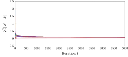
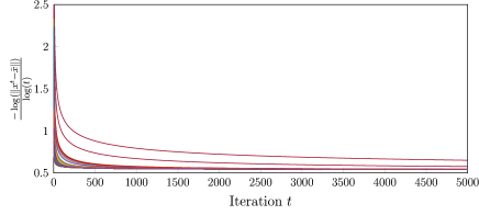
Fig. 1: Numerical simulation results: (top) the successive change $\sqrt[4]{t}\,\|x^{t}-\bar{x}\|$ and (bottom) the ratio $\frac{-{\log(\|x^{t}-\bar{x}\|)}}{\log(t)}$ as a function of the number of iterations, $t$.

From the first graph, we see that the value of $\sqrt[4]{t}\,\|x^{t}-\bar{x}\|$ quickly decreases with increasing $t$. This supports the result that $x^{t}$ converges at least in the order of $O(1/\sqrt[4]{t})$. From the second graph, the value of $\frac{-{\log(\|x^{t}-\bar{x}\|)}}{\log(t)}$ appears to approach $1/2$. This suggests that the actual sublinear convergence rate for this example is $O(1/\sqrt{t})$, regardless of the choice of the initial point.

Furthermore, the following example shows that, whenever the initial point is chosen in the region specified below, the sequence in Example 6.50 converges with an exact order $O(1/\sqrt{t})$ and thus supports the conjectured rate of convergence.

Example 6.51 (The sequence in Example 6.50 with specific initial points).

Consider the setting of Example 6.50, and suppose that the initial point $x^{0}=(u_{0},v_{0})\in\mathbb{R}_{--}\times(0,1)$. If $x^{t}=(u_{t},v_{t})\in\mathbb{R}_{--}\times(0,1)$, then using (32) we deduce that

$$x^{t+1}=T_{C,D}(x^{t})=\frac{(1-u_{t},v_{t})}{\sqrt{(1-u_{t})^{2}+v_{t}^{2}}}-(1,0)\in\mathbb{R}_{--}\times(0,1).$$

Inductively, the Douglas–Rachford sequence $\{x^{t}\}$ is contained in $\mathbb{R}_{--}\times\mathbb{R}_{++}$. By Example 6.50, the sequence $x^{t}=(u_{t},v_{t})\rightarrow(0,0)$. Below we verify that the sequence with an exact sublinear convergence order $O(1/\sqrt{t})$.

To see this, we note from $u_{t}<0$ that

$$v_{t+1}=\frac{v_{t}}{\sqrt{(1-u_{t})^{2}+v_{t}^{2}}}<\frac{v_{t}}{\sqrt{1+v_{t}^{2}}}.$$

Setting $w_{t}=:v_{t}^{2}$, we deduce

$$w_{t+1}<\frac{w_{t}}{1+w_{t}}=w_{t}-w_{t}^{2}+O(w_{t}^{3}).$$

Since $w_{t}\to 0$, for sufficiently large $t$, we have

$$w_{t+1}<w_{t}-\frac{1}{2}w_{t}^{2}\implies\frac{1}{w_{t+1}}-\frac{1}{w_{t}}>\frac{1}{2-w_{t}}\implies\liminf_{t\to\infty}\left(\frac{1}{w_{t+1}}-\frac{1}{w_{t}}\right)\geq\frac{1}{2}.$$

It now follows that

$$\left(\liminf_{t\to\infty}\frac{1/\sqrt{t}}{v_{t}}\right)^{2}=\liminf_{t\to\infty}\frac{1}{t}\frac{1}{w_{t}} =\liminf_{t\to\infty}\frac{1}{t}\left(\frac{1}{w_{t}}-\frac{1}{w_{0}}\right)$$

$$=\liminf_{t\to\infty}\frac{1}{t}\sum_{n=0}^{t-1}\left(\frac{1}{w_{n+1}}-\frac{1}{w_{n}}\right)\geq\frac{1}{2}.$$

Taking square roots and inverting both sides we obtain

(37) $$\limsup_{t\to\infty}\frac{v_{t}}{1/\sqrt{t}}\leq\sqrt{2}.$$

Now, recall that

$$u_{t+1}=\frac{1-u_{t}}{\sqrt{(1-u_{t})^{2}+v_{t}^{2}}}-1 = \frac{(1-u_{t})-\sqrt{(1-u_{t})^{2}+v_{t}^{2}}}{\sqrt{(1-u_{t})^{2}+v_{t}^{2}}}$$

$$= \frac{-v_{t}^{2}}{\sqrt{(1-u_{t})^{2}+v_{t}^{2}}\big{(}(1-u_{t})+\sqrt{(1-u_{t})^{2}+v_{t}^{2}}\big{)}}.$$

Since $\sqrt{(1-u_{t})^{2}+v_{t}^{2}}\big{(}(1-u_{t})+\sqrt{(1-u_{t})^{2}+v_{t}^{2}}\big{)}\rightarrow 2$ as $t\rightarrow\infty$, whenever $t$ is sufficiently large we have

(38) $$0>u_{t+1}\geq-v_{t}^{2}.$$

Combining (37) and (38), we see that there exists $C>0$ such that $\|(u_{t},v_{t})\|\leq C\frac{1}{\sqrt{t}}$ for all $t\in\mathbb{N}$. In particular, this also shows that $u_{t}\rightarrow 0$.

Noting that $\frac{v_{t+1}}{v_{t}}=\frac{1}{\sqrt{(1-u_{t})^{2}+v_{t}^{2}}}\to 1$ as $t\to\infty$ and $v_{t}>0$, we therefore deduce that $v_{t-1}<2v_{t}$ for all sufficiently large $t$. Combined with (38), this yields

$$v_{t+1}=\frac{v_{t}}{\sqrt{(1-u_{t})^{2}+v_{t}^{2}}}\geq\frac{v_{t}}{\sqrt{(1+v_{t-1}^{2})^{2}+v_{t}^{2}}}=\frac{v_{t}}{\sqrt{1+9v_{t}^{2}+16^{2}v_{t}^{4}}}>\frac{v_{t}}{1+\frac{9}{2}v_{t}^{2}}.$$

As before, we set $w_{t}:=v_{t}^{2}$. Since $w_{t}\to 0$ and $(1+\frac{9}{2}w_{t})^{2}(1-10w_{t})=1-w_{t}-\frac{279}{4}w_{t}^{2}-\frac{405}{2}w_{t}^{3}<1$, we deduce

$$w_{t+1}>\frac{w_{t}}{(1+\frac{9}{2}w_{t})^{2}}>w_{t}(1-10w_{t})\implies w_{t+1}>w_{t}-10w_{t}^{2}.$$

Proceeding as before, we obtain

$$\liminf_{t\to\infty}\frac{v_{t}}{1/\sqrt{t}}\geq\frac{1}{10}.$$

This shows that $\|(u_{t},v_{t})\|\geq\frac{1}{10}\,\frac{1}{\sqrt{t}}$. Altogether, we have proven that $(u_{t},v_{t})\rightarrow(0,0)$ with an exact sublinear convergence order $O(1/\sqrt{t})$.

7 Conclusions

In this paper, using a Hölder regularity assumption, sublinear and linear convergence of fixed point iterations described by averaged nonexpansive operators has been established. The framework was then specialized to various fixed point algorithms including Krasnoselskii–Mann iterations, the cyclic projection algorithm, and the Douglas–Rachford feasibility algorithm along with some variants. In the case where the underlying sets are convex semi-algebraic, in a finite dimensional space, the results apply without any further regularity assumptions.

In particular, for our damped Douglas–Rachford algorithm, an explicit estimate for the sublinear convergence rate has been provided in terms of the dimension and the maximum degree of the polynomials which define the convex sets. We emphasize that, unlike the for damped Douglas–Rachford algorithm, we were not able to provide an explicit estimate of the sublinear convergence rate for the classical Douglas–Rachford algorithm when the two convex sets are described by convex polynomials. Our approach relies on the Łojasiewicz’s inequality which gives no quantitative information regarding the Hölder exponent. Providing explicit estimates is left as an open question for future research.

Another area for future research involves characterization of the convergence rate in the absence of Hölder regularity properties. For instance, it is known that the alternating projection method can exhibit arbitrarily slow convergence when applied to two subspaces in infinite dimensional spaces without closed sum [13]. As shown in [20, Cor. 3.1], if only two sets are involved and the initial point is chosen in a specific way, the cyclic Douglas–Rachford method can coincide with the alternating projection method, and so, it may exhibit arbitrarily slow convergence. On the other hand, it was shown in Proposition 4.34 that the basic/cyclic Douglas–Rachford method enjoys a sublinear convergence rate if the underlying sets are convex semi-algebraic sets in finite dimensional spaces. It would be interesting to see whether an arbitrarily slow convergence can happen for these two methods for general closed and convex sets in finite dimensional spaces.

Finally, the current definition of basic semi-algebraic convex sets only applies to finite dimensional spaces. It would interesting to see if a suitable extension of the notion can be profitably used in infinite dimensional spaces using, for instance, polynomials as defined in [30].

Acknowledgments

JMB is supported, in part, by the Australian Research Council. GL is supported, in part, by the Australian Research Council. MKT is supported by Deutsche Forschungsgemeinschaft Research Training Grant 2088. The work was partially performed during his candidature at the University of Newcastle where he was supported by an Australian Postgraduate Award. The authors wish to thank Neal Hermer, Victor Isaac Kolobov, Simeon Reich, Rafał Zalas and the three anonymous referees for their insightful comments.

References

- [1] F.J. Aragón Artacho, J.M. Borwein and M.K. Tam, Douglas–Rachford feasibility methods for matrix completion problems, ANZIAM J., 55 (2014), pp. 299–326.
- [2] F.J. Aragón Artacho, J.M. Borwein and M.K. Tam, Recent results on Douglas–Rachford methods for combinatorial optimization problems, J. Optim. Theory Appl., 163 (2014), pp. 1–30.
- [3] H. Attouch, J. Bolte, P. Redont and A. Soubeyran, Proximal alternating minimization and projection methods for nonconvex problems: an approach based on the Kurdyka-Łojasiewicz inequality, Math. Oper. Res., 35 (2010), pp. 438-457.
- [4] J.-B. Baillon, R. E. Bruck and S. Reich, On the asymptotic behavior of nonexpansive mappings and semigroups in Banach spaces, Houston J. Math. 4 (1978), pp. 1–9.
- [5] H.H. Bauschke and J.M. Borwein, On the convergence of von Neumann’s alternating projection algorithm for two sets, Set-Valued Anal., 1 (1993), pp. 185–212.
- [6] H.H. Bauschke and J.M. Borwein, On projection algorithms for solving convex feasibility problems, SIAM Rev., 38 (1996), pp. 367–426.
- [7] H.H. Bauschke and P.L. Combettes, Convex analysis and monotone operator theory in Hilbert spaces, Springer-Verlag, New York, 2011.
- [8] H.H. Bauschke, P.L. Combettes and S.G. Kruk, Extrapolation algorithm for affine-convex feasibility problems, Numer. Alg., 41 (2006), pp. 239–274.
- [9] H.H. Bauschke, P.L. Combettes and D.R. Luke, Finding best approximation pairs relative to two closed convex sets in Hilbert spaces, J. Approx. Theory, 127 (2004), pp. 179–192.
- [10] H. Bauschke, D. Noll and H.M. Phan, Linear and strong convergence of algorithms involving averaged nonexpansive operators, J. Math. Anal. Appl., 421 (2015), pp. 1–20.
- [11] H. Bauschke, J. B. Cruz, T.T. Nghia, H.M. Phan and X. Wang, The rate of linear convergence of the Douglas–Rachford algorithm for subspaces is the cosine of the Friedrichs angle, J. Approx. Theory, 185 (2014), pp. 63–79.
- [12] H.H. Bauschke, M.N. Dao, D. Noll and H.M. Phan, Proximal point algorithm, Douglas–Rachford algorithm and alternating projections: a case study, J. Convex Anal., in press.
- [13] H.H. Bauschke, F. Deutsch and H. Hundal, Characterizing arbitrarily slow convergence in the method of alternating projections, Int. Trans. Oper. Res., 16 (2009), pp. 413–425.
- [14] J. Bochnak, M. Coste and M.F. Roy, Real algebraic geometry, Springer-Verlag, Berlin, 1998.
- [15] J.M. Borwein, Maximum entropy and feasibility methods for convex and nonconvex inverse problems, Optim. 61 (2012), pp. 1–33.
- [16] J.M. Borwein and B. Sims, The Douglas–Rachford algorithm in the absence of convexity, in Fixed-Point Algorithms for Inverse Problems in Science and Engineering, H.H. Bauschke, R. Burachik, P.L. Combettes, V. Elser, D.R. Luke and H. Wolkowicz, eds., Springer-Verlag, New York, 2011, pp. 93–109.
- [17] J.M. Borwein, G.Li and L.J. Yao, Analysis of the convergence rate for the cyclic projection algorithm applied to basic semi-algebraic convex sets, SIAM J. Optim., 24 (2014), pp. 498–527.
- [18] J.M. Borwein, B. Sims and M.K. Tam, Norm convergence of realistic projection and reflection methods, Optim. 64 (2015), pp. 161–178.
- [19] J.M. Borwein and M.K. Tam, The cyclic Douglas–Rachford method for inconsistent feasibility problems, J. Nonlinear Convex Anal., 16 (2015), pp. 537–584.
- [20] J.M. Borwein and M.K. Tam, A cyclic Douglas–Rachford iteration scheme, J. Optim. Theory Appl., 160 (2014), pp. 1–29.
- [21] Y. Censor and A. Cegielski, Projection methods: an annotated bibliography of books and reviews, Optim., 64 (2015), pp. 2343–2358.
- [22] P.L. Combettes, The convex feasibility problem in image recovery, Adv. Imaging Electron Phys., 95 (1996), pp. 155–270.
- [23] P. L. Combettes Solving monotone inclusions via compositions of nonexpansive averaged operators, Optim., 53 (2004), no. 5-6, pp. 475–504.
- [24] D. Davis, Convergence rate analysis of the forward-Douglas–Rachford splitting scheme, SIAM J. Optim., 25 (2015), pp. 1760–1786.
- [25] D. Davis and W. Yin, Convergence rate analysis of several splitting schemes, \hrefhttp://arxiv.org/abs/1406.4834v3arXiv:1406.4834v3, (2015).
- [26] D. Drusvyatskiy and A.S. Lewis, Semi-algebraic functions have small subdifferentials, Math. Program., 140 (2013), pp. 5–29.
- [27] R. Escalante and M. Raydan, Alternating projection methods, SIAM, Philadelphia, PA, 2011.
- [28] P. Giselsson, Tight global linear convergence rate bounds for Douglas–Rachford splitting \hrefhttp://arxiv.org/abs/arXiv:1506.01556arXiv:1506.01556, (2015).
- [29] L.G. Gubin, B.T. Polyak, and E.V. Raik, The method of projections for finding the common point of convex sets, USSR Comp. Math. Math.+, 7 (1967), pp. 1–24.
- [30] J.M. Gutiérrez, J.A. Jaramillo, and J.G. Llavona, Polynomials and geometry of Banach spaces, Extracta Math., 10 (1995), p. 77–114.
- [31] A.Y. Kruger. Error bounds and metric subregularity, Optim., 64 (2015), pp. 49–79.
- [32] A.Y. Kruger and Nguygen H.T, About -regularity properties of collections of sets, J. Math. Anal. Appl., 416 (2014), pp. 471–496.
- [33] G. Li, On the asymptotic well behaved functions and global error bound for convex polynomials, SIAM J. Optim., 20 (2010), pp. 1923–1943.
- [34] G. Li, Global error bounds for piecewise convex polynomials, Math. Program., 137 (2013), pp. 37–64.
- [35] G. Li and B.S. Mordukhovich, Hölder metric subregularity with applications to proximal point method, SIAM J. Optim., 22 (2012), pp. 1655–1684.
- [36] G. Li and T. K. Pong Douglas-Rachford splitting for nonconvex optimization with application to nonconvex feasibility problems, to appear in Math. Program., (2016), DOI: 10.1007/s10107-015-0963-5.
- [37] J. Douglas and H.H. Rachford, On the numerical solution of heat conduction problems in two or three space variables, Trans. Amer. Math. Soc., 82 (1956), pp. 421–439.
- [38] J. Eckstein and D.P. Bertsekas, On the Douglas–Rachford splitting method and the proximal point algorithm for maximal monotone operators, Math. Program., 55 (1992), pp. 293–318.
- [39] R. Hesse and D.R. Luke, Nonconvex notions of regularity and convergence of fundamental algorithms for feasibility problems, SIAM J. Optim., 23 (2013), pp. 2397–2419.
- [40] R. Hesse, D.R. Luke and P. Neumann, Alternating projections and Douglas–Rachford for sparse affine feasibility, IEEE Trans. Signal Process. 62 (2014), pp. 4868–4881.
- [41] A.S. Lewis, D.R. Luke and J. Malick, Local convergence for alternating and averaged nonconvex projections, Found. Comput. Math., 9 (2009), pp. 485–513.
- [42] A.S. Lewis and J. Malick, Alternating projections on manifolds, Math. Oper. Res., 33 (2008), pp. 216–234.
- [43] P.-L. Lions and B. Mercier, Splitting algorithms for the sum of two nonlinear operators, SIAM J. Numer. Anal., 16 (1979), pp. 964–979.
- [44] D.R. Luke, Finding best approximation pairs relative to a convex and a prox-regular set in a Hilbert space, SIAM J. Opt., 19(2008), pp. 714–739.
- [45] H. Phan, Linear convergence of the Douglas–Rachford method for two closed sets, Optim., online first (2015). doi: 10.1080/02331934.2015.1051532.
- [46] B.F. Svaiter, On weak convergence of the Douglas–Rachford method, SIAM J. Control Optim., 49 (2011), pp. 280–287.
- [47] E.D. Sontag, Remarks on piecewise-linear algebra, Pacific J. Math., 98 (1982), pp. 183–201.
- [48] S. Reich and R. Zalas, A modular string averaging procedure for solving the common fixed point problem for quasi-nonexpansive mappings in Hilbert space, Numer. Algorithms, 72 (2016), 297–323.
- [49] S.M. Robinson, Some continuity properties of polyhedral multifunctions, in Mathematical Programming at Oberwolfach vol. 14, Springer Berlin Heidelberg, 1981, pp. 206–214.