Cluster–Void Degeneracy Breaking: Dark Energy, Planck, and the Largest Cluster & Void

Abstract

Combining galaxy cluster and void abundances breaks the degeneracy between mean matter density $\Omega_{\rm m}$ and power spectrum normalization $\sigma_{8}$. In a first for voids, we constrain $\Omega_{\rm m}=0.21\pm 0.10$ and $\sigma_{8}=0.95\pm 0.21$ for a flat $\Lambda$CDM universe, using extreme-value statistics on the claimed largest cluster and void. The Planck-consistent results detect dark energy with two objects, independently of other dark energy probes. Cluster–void studies also offer complementarity in scale, density, and non-linearity – of particular interest for testing modified-gravity models.

1 INTRODUCTION

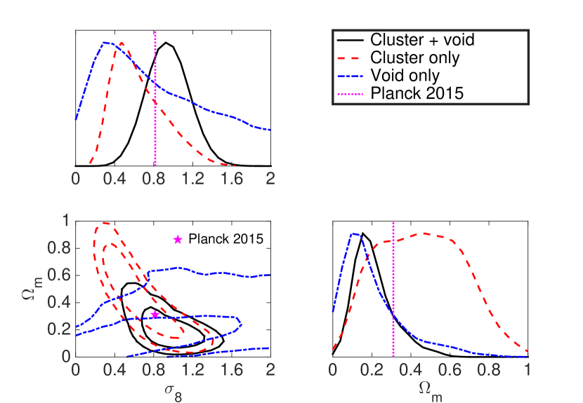
Figure 1: Survey-patch constraints on $\Omega_{\rm m}$ and $\sigma_{8}$ ($68\%$ and $95\%$ confidence levels) from the largest cluster and void individually (red dashed, blue dash-dotted lines) and jointly (black solid lines).

Clusters and voids in the galaxy distribution are rare extremes of the cosmic web. As sensitive probes of the statistics of the matter distribution, they are useful tools for testing cosmological models. The abundances of clusters and voids are sensitive probes of dark energy (Pisani et al. 2015; Allen et al. 2011), modified gravity (Lam et al. 2015; Allen et al. 2011), neutrino properties (Brandbyge et al. 2010; Massara et al. 2015), and non-Gaussianity (Chongchitnan & Silk 2010).

Tests of the consistency of the most massive clusters with concordance $\Lambda$CDM cosmology have been performed over the last 20 years (Bahcall & Fan 1998; Hoyle et al. 2011; Mortonson et al. 2011; Harrison & Hotchkiss 2013). No statistically significant tension prevails between the existence of the most massive clusters and concordance cosmology. Large and deep voids have been considered as a possible problem for concordance cosmology (Peebles 2001; Xie et al. 2014; Chongchitnan 2015). While there are indications of possible discrepancies with $\Lambda$CDM, the significance of these is unclear. Only recently, sufficiently large and deep galaxy surveys enabled study of the statistics of the largest voids (e.g. Sutter et al. 2012; Nadathur & Hotchkiss 2014).

Chongchitnan (2015) studied the expected largest voids in concordance cosmology, and concludes some tension between expectation and observation. The use of void abundances to constrain $\sigma_{8}$ and $\Omega_{\rm m}h$ was discussed by Betancort-Rijo et al. (2009), but they did not derive constraints, nor study the complementarity with cluster abundances. Pisani et al. (2015) explored future dark energy constraints from void abundances, and qualitatively argued for complementarity with cluster abundances. A joint cluster-void analysis and real-data cosmological parameter inference based on void abundance is still outstanding.

This work evaluates the complementarity of cluster and void abundances as cosmological probes, through analyzing whether the existence of the largest cluster and void is individually and/or jointly consistent with Planck cosmology (Planck collaboration 2015). This includes the first quantitative cosmological parameter estimation based on void abundances. We find that cluster and void abundances powerfully break each other’s parameter degeneracies, similar to complementarity between clusters and the cosmic microwave background (CMB). We explicitly model the effect of massive neutrinos, and Eddington bias in observables.

2 DATA

We use data for the claimed largest galaxy cluster and void found so far. The surveys are summarized in Table 1. We also investigate an ‘observable Universe’ case covering $z=0-6$.

Table 1: Survey specifications.

Survey	Area [sq. deg.]	Redshift
Cluster (ACT)	$1000$	$0.3-6$
Void (WISE–2MASS)	$21200$	$0-0.3$

2.1 Cluster

A handful of galaxy clusters are ‘most massive known’ candidates. We choose ACT-CL J0102-4915 ‘El Gordo’ (Menanteau et al. 2012), which has a weak-lensing mass estimate that spans the range of uncertainty for the candidate set. It is most massive for at least $z>0.6$, and its equivalent redshift-zero mass is most extreme (Harrison & Hotchkiss 2013).

‘El Gordo’ was discovered by the Atacama Cosmology Telescope (ACT) collaboration at a spectroscopic redshift $z=0.87$ through its Sunyaev–Zel’dovich (SZ) signal. The survey area is 1000 sq. deg. (Hasselfield et al. 2013). It is estimated complete for $M_{200}~{}>~{}8~{}\times~{}10^{14}h^{-1}M_{\odot}$ in $z=0.3-6$ (Harrison & Hotchkiss 2013). The strongest SZ decrement in the survey patch corresponds to the cluster (Hasselfield et al. 2013). We assume it is the most massive halo in the survey patch. We use the Hubble Space Telescope weak-lensing mass measurement by Jee et al. (2014), $M_{200}=\left(2.19\pm 0.78\right)\times 10^{15}h^{-1}M_{\odot}$ (incl. syst. unc.).

2.2 Void

A supervoid (quasi-linear void) claimed the largest known was recently identified at $z=0.22\pm 0.03$, as a galaxy underdensity in the WISE–2MASS infrared galaxy catalogue (Szapudi et al. 2014a). The void is aligned with the Cold Spot (CS) in the CMB (Finelli et al. 2014), hence we call it the ‘CS Void’. The survey area is 21200 sq. deg. (Kovács & Szapudi 2014), across $z=0-0.3$ (Szapudi et al. 2014b). No underdensity of larger size was identified in the survey (Szapudi et al. 2014b). We assume it is the largest void in the survey patch. Szapudi et al. (2014a) measure a comoving radius $R=\left(220\pm 50\right)h^{-1}$Mpc (in galaxy density) and a cold-dark-matter density contrast $\delta^{\rm cdm}_{\rm v}=-0.14\pm 0.04$, after accounting for galaxy bias. The assumed fiducial $\Lambda$CDM model is $\Omega_{\rm m}=0.3,\Omega_{\Lambda}=0.7,h=0.7$ (Kovács 2015). We rescale the observed radius as $R=R_{\rm fiducial}[(dV/dz)/(dV/dz)_{\rm fiducial}]^{1/3}$ (Pisani et al. 2015). Void parameters are defined for a real-space top-hat model. We assume the survey is complete for voids of similar or larger size (Kovács & Szapudi 2014). For a large void partly contained in the survey, the density profile will be misestimated, but should be detected. A void covering the survey volume may be undetectable, but such voids ($R>600\,h^{-1}$ Mpc) should occur once in $>10^{8}$ Hubble volumes. Void numbers are exponentially suppressed with radius. Hence, Eq. (1), below, is insensitive to selection for voids much larger than the lower integration limit. Voids less underdense than the CS Void are not relevant for our analysis.

3 METHOD

3.1 Model

We predict cluster and void abundances adapting standard methodology (Sahlén et al. 2009).

Cosmological Model

We assume a flat $\Lambda$CDM model with a power-law power spectrum of primordial density perturbation, and massive neutrinos. The model is specified by today’s values of mean matter density $\Omega_{\rm m}$, mean baryonic matter density $\Omega_{\rm b}$, sum of neutrino masses $\Sigma m_{\nu}$, statistical spread of the matter field at quasi-linear scales $\sigma_{8}$, and scalar spectral index $n_{\rm s}$. We assume $\Sigma m_{\nu}=0.06\,{\rm eV}$, one neutrino mass eigenstate and three neutrino species so that the effective relativistic degrees of freedom $N_{\rm eff}=3.046$.

Number Counts

The model for number counts is

$$N_{\rm obs}=\int\int\int p(O|O_{\rm t})n[M(O_{\rm t}),z]\frac{dM}{dO_{\rm t}}\frac{dV}{dz}dzdO_{\rm t}dO,$$ (1)

where $O$ is the size observable (mass, radius) for a type of object (here cluster or void), $O_{\rm t}$ the true physical value of the observable $O$, and $M(O_{\rm t})$ the mass of the object. The differential number density is given by $n(M,z)$, $p(O|O_{\rm t})$ is the measurement pdf for the observable $O$, and $dV/dz$ is the cosmic volume element. For integrating Eq. (1), we use $M_{\rm void}=\frac{4}{3}\pi R^{3}\rho_{\rm m}(1+\delta^{\rm m}_{\rm v})$. We highlight that while we write the expression for voids in terms of a mass, they are observationally defined by radius and density contrast. Redshift integration is performed according to survey specifications (Table 1), or ‘observable Universe’ specification.

Number Density

The differential number density of objects in a mass interval ${\rm d}M$ about $M$ at redshift $z$ is

$$n(M,z)\,{\rm d}M=-F(\sigma,z)\,\frac{\rho_{\rm m}(z)}{M\sigma(M,z)}\,\frac{{\rm d}\sigma(M,z)}{{\rm d}M}\,{\rm d}M\,,$$ (2)

where $\sigma(M,z)$ is the dispersion of the density field at some comoving scale $R_{L}=(3M/4\pi\rho_{\rm m})^{1/3}$, and $\rho_{\rm m}(z)=\rho_{\rm m}(z=0)(1+z)^{3}$ the matter density. The expression can be written in terms of linear-theory radius $R_{L}$ for voids. The multiplicity function (MF) denoted $F(\sigma,z)$ is described in the following for clusters and voids.

Cluster MF

The cluster (halo) MF $F_{h}(\sigma)$ encodes the halo collapse statistics. We use the MF of Watson et al. (2013), their Eqs. (12)-(15), accurate to within $10\%$ for the regime we consider. Since our measured mass is defined at overdensity $200$ (rather than 178), we convert to a $\Delta=200$ overdensity using a scaling relation, their Eqs. (17)-(19) (Watson et al. 2013).

Neutrinos are treated according to Brandbyge et al. (2010). Neutrinos free-stream on cluster scales, and do not participate in gravitational collapse, so cluster masses should be rescaled: $M=4\pi R^{3}_{L}[(1-f_{\nu})\rho_{\rm m}+f_{\nu}\rho_{\rm b}]/3$, where $f_{\nu}=[\Sigma m_{\nu}/93\,{\rm eV}]/\Omega_{\rm dm}h^{2}$ is the fraction of dark matter abundance $\Omega_{\rm dm}$ in neutrinos, and $\rho_{\rm b}$ is the baryon density. This gives a good first-order approximation, used with massless-neutrino MFs. Massive neutrinos also affect cluster and void distributions by shifting the turn-over scale in the matter power spectrum, and suppression of power on the neutrino free-streaming scale.

Void MF

The theoretical description of the void MF is not robustly known, mainly due to ambiguities in void definition, dynamics, and selection (e.g. Chongchitnan 2015). We use the Sheth–van de Weygaert (SvdW) MF (Sheth & van de Weygaert 2004) based on excursion set theory, but adapt it to supervoids, to describe a first-crossing distribution for voids with a particular density contrast $\delta_{\rm v}$. Void-in-cloud statistics are unimportant for our size of void. We pick the SvdW MF as representative also of alternative void MFs for our range of parameter values.

Achitouv et al. (2015) show that several spherical-expansion + excursion set theory predictions of the void MF consistently describe the dark-matter void MF from $N$-body simulations within simulation uncertainties across at least $R=1-10\,h^{-1}$ Mpc. The SvdW MF is defined for a top-hat filter in momentum space. The observation is defined in real space, which introduces non-Markovian corrections. Achitouv et al. (2015) derive a ‘DDB’ void MF including such corrections, and stochasticity in the void formation barrier. We have computed that these corrections give a $\sim 10\%$ increase in the void MF compared to SvdW for $R>100\,h^{-1}$ Mpc and $\delta_{\rm v}>-0.3$. The SvdW MF predicts $\mathcal{O}(1)$ voids with $R\sim 200\,h^{-1}$ Mpc in the WISE–2MASS survey patch, consistent with the peaks-theory prediction by Nadathur et al. (2014) rescaled to the survey patch, and extreme-void statistics in the largest $N$-body simulations (e.g. Hotchkiss et al. 2015). Large, small-underdensity voids should be close to linear and trace initial underdensity peaks, and hence not so sensitive to expansion dynamics and interactions. Indeed, the excursion-set-peaks prediction (Paranjape & Sheth 2012) falls inbetween the SvdW and DDB MFs. Thus, SvdW should be a good approximation to the dark-matter void MF to within $\lesssim 50\%$. This uncertainty is significantly smaller than the Poisson uncertainty and propagated uncertainty in radius. These considerations motivate interest in a supervoid, rather than fully non-linear void.

While there is no consensus on the normalization of the dark-matter void MF, its shape is relatively well-understood for large supervoids. The same applies to voids defined by biased tracers such as galaxies, provided $\delta_{\rm v}$ is calibrated to survey specifications (Pisani et al. 2015). The radius and density contrast defined from tracers are larger than corresponding dark-matter quantities. Since we use a dark-matter density contrast, but a galaxy-density radius, we choose a converse approach. We set $\delta_{\rm v}$ to the measured dark-matter value (within uncertainties), and allow the radius to be self-calibrated (Hu 2003) to a dark-matter radius by the data. This procedure is successful in that only void radius but not density contrast is re-calibrated in parameter estimation. This is analogous to the scaling-relation strategy used for galaxy clusters (Allen et al. 2011).

The void MF for (non-linear) radius $R$ should be evaluated at corresponding linear radius $R_{\rm L}$, related as $R/R_{\rm L}=(1+\delta^{\rm m}_{\rm v})^{-1/3}$, with $\delta^{\rm m}_{\rm v}$ non-linear. The linear density contrast $\delta_{\rm L}$ defines the MF density threshold. We approximate the spherical-expansion relationship by $\delta^{\rm m}_{\rm v,L}=c[1-(1+\delta^{\rm m}_{\rm v})^{-1/c}]$, $c=1.594$ (Jennings et al. 2013).

Neutrinos are treated according to Massara et al. (2015). Neutrino density contributes to the dynamical evolution of the void, but lacks significant density contrast itself. We use $\delta^{\rm m}_{\rm v}=[1-f_{\nu}(1+\Omega_{\rm b}/\Omega_{\rm m})]\delta^{\rm cdm}_{\rm v}$, where $\delta^{\rm cdm}_{\rm v}$ is the cold-dark-matter density contrast (which is our observational quantity).

Measurement Uncertainty

We use a log-normal pdf $p(O|O_{\rm t})$ in Eq. (1) for the observable $O$ (i.e. $M_{200}$ or $R$) given its true value $O_{\rm t}$, with the mean and variance matched to the mean and variance of the observational cluster mass or void radius determinations, $\mu_{\ln O}=\ln O_{\rm t}/\sqrt{1+(\sigma_{O}/O_{\rm t})^{2}}$ and $\sigma^{2}_{\ln O}=\ln[1+(\sigma_{O}/O_{\rm t})^{2}]$. This approximation does not bias predicted abundances. Including this probability distribution in predictions corrects for the otherwise-present Eddington bias. We also perform an Eddington-biased analysis for which $p(O|O_{\rm t})=\delta(O-O_{\rm t})$. Redshift uncertainties are neglected, as they are contained in the survey patches.

3.2 LIKELIHOOD

Cluster–Void Extreme Value Statistics

Number counts follow Poisson statistics, corrected for object-to-object clustering. The fractional correction to Poisson counts due to mild $[N_{\rm c}(>M)\ll 1]$ clustering is $-N_{\rm c}(>M)/2$ (Colombi et al. 2011), where $N_{\rm c}(>M)\equiv\bar{\xi}(>M)N(>M)$, and $\bar{\xi}(>M)$ is the average auto- or cross-correlation for objects above the mass threshold(s) within the patch. For all our cluster and void cases, we estimate $N_{\rm c}(>M)\lesssim 0.01$, based on Davis et al. (2011), and correlation function and bias results in Sheth & van de Weygaert (2004); Hamaus et al. (2014); Clampitt et al. (2016). Hence, our number counts follow non-clustered Poisson statistics to sub-percent-level accuracy.

Extreme value (or Gumbel) statistics describe the pdf of extrema of samples drawn from random distributions (Gumbel 1958). Consider a large patch of the Universe, populated with clusters and voids. Let $M_{\rm max}$ be the mass of the most extreme cluster (or void), and $p_{\rm G}\left(M_{\rm max}\right)$ be the pdf of $M_{\rm max}$. For non-clustered Poisson statistics, we can write (Davis et al. 2011; Colombi et al. 2011):

$$p_{\rm G}\left(M\right)=\frac{dN(>M)}{dM}e^{-N(>M)}\,,$$ (3)

where $N(>M)$ is the mean number of clusters (or voids) above the threshold $M$ within the patch, according to Eq. (1). The total Gumbel likelihood (under non-clustering) is then

$$p_{\rm G}(M_{\rm halo},M_{\rm void})=p^{\rm halo}_{\rm G}\left(M_{\rm halo}\right)p^{\rm void}_{\rm G}\left(M_{\rm void}\right)\,.$$ (4)

This likelihood is multiplied with measurement pdfs and external priors, and evaluated as described in Sec. 3.3.

Measurement Uncertainty

We include measurement uncertainties in cluster and void properties as normally distributed with means and variances as detailed in Sec. 2.

External Priors

In line with recent Planck analyses (Planck collaboration 2015), we use the following external priors:

$$h =0.706\pm 0.033\,\,\text{\rm(maser+Cepheids,\,{\cite[citet]{\@@bibref{Authors Phrase1YearPhrase2}{2014MNRAS.440.1138E}{\@@citephrase{}}{\@@citephrase{}}}})}\,,$$ (5)

$$\Omega_{\rm b}h^{2} =0.023\pm 0.002\,\,\text{\rm(BBN,\,{\cite[citet]{\@@bibref{Authors Phrase1YearPhrase2}{Agashe:2014kda}{\@@citephrase{}}{\@@citephrase{}}}})}\,,$$ (6)

$$n_{\rm s} =0.9677\pm 0.006\,\,\text{\rm(CMB,\,{\cite[citet]{\@@bibref{Authors Phrase1YearPhrase2}{Planck2015}{\@@citephrase{}}{\@@citephrase{}}}})}\,,$$ (7)

$$\Sigma m_{\nu} =0.06\,\text{\rm eV\,(1\,mass\,eigenstate)\,\,(NO,\, {\cite[citet]{\@@bibref{Authors Phrase1YearPhrase2}{Agashe:2014kda}{\@@citephrase{}}{\@@citephrase{}}}})}\,,$$ (8)

$$N_{\rm eff} =3.046\,\,\text{\rm(Std.\,Model, 3\,neutrino\,species)}\,.$$ (9)

We specify $T_{\rm CMB}=2.7255$ K (Fixsen 2009) for the radiation energy density. With these priors, our analysis is directly comparable to the Planck results. For an equivalent analysis independent of CMB anisotropies, we can set $n_{\rm s}\approx 1$ assuming an inflationary origin of primordial perturbations, or based on large-scale-structure surveys.

3.3 Computation

We perform Monte Carlo Markov Chain parameter estimation on the parameter space $\{h,\Omega_{\rm m},\Omega_{\rm b},\sigma_{8},$ $n_{\rm s},R_{\rm eff},\delta^{\rm cdm}_{\rm v},M_{200}\}$, where $R_{\rm eff}$ is the effective self-calibrated dark-matter void radius. The likelihood, Eq. (4) $\times$ measurement pdfs $\times$ priors, is evaluated using a modified version of CosmoMC (Lewis & Bridle 2002), employing techniques in Sahlén et al. (2009). Abundances are computed using CUBPACK (Cools & Haegemans 2003).

4 RESULTS

4.1 Number Counts

In a Planck cosmology, we predict in the survey patches an Eddington-biased (unbiased) mean number of clusters $N(>M_{200})$ in the range $[10^{-2},87]\,([10^{-4},49])$, and mean number of voids $N(>R)$ in the range $[10^{-11},22]\,([10^{-100},20])$. These correspond to $2\sigma$ CIs of cluster and void properties.

Massive neutrinos produce a relatively insignificant suppression in mean Eddington-biased numbers. The unbiased means in the above cases are suppressed between $\sim 5-50\%$.

4.2 Cosmological Parameters

Parameter contours for $\Omega_{\rm m}$ and $\sigma_{8}$ are shown in Fig. 1, and marginalized constraints in Table 2. Planck concordance cosmology is inside the $68\%$ confidence contours for the cluster-only and cluster+void cases, and the $95\%$ contours for the void-only case. The objects are individually and mutually consistent with concordance cosmology. The joint analysis detects dark energy at $>7\sigma$.

Table 2: Marginalized means for $\Omega_{\rm m}$ and $\sigma_{8}$ (with $68\%$ CIs), and best-fit values, in the joint cluster–void analysis.

	Eddington-corrected		Eddington-biased
Case	$\Omega_{\rm m}$	$\sigma_{8}$	$\Omega_{\rm m}$	$\sigma_{8}$
Survey	$0.21\pm 0.10$ $0.27$	$0.95\pm 0.21$ $0.82$	$0.22\pm 0.12$ $0.15$	$0.99\pm 0.22$ $1.17$
Observable Universe $z=0-6$	$0.23\pm 0.11$ $0.32$	$0.70\pm 0.14$ $0.72$	$0.21\pm 0.08$ $0.20$	$0.78\pm 0.13$ $0.80$

4.3 Self-calibration

The void radius is consistently self-calibrated to a dark-matter-field radius of $R_{\rm eff}=184\pm 51\,h^{-1}$ Mpc in the Eddington-corrected survey-patch analysis, with the density-contrast pdf preserved.

4.4 Eddington Bias

Eddington bias does not significantly affect the constraints. The bias, if unaccounted for, is a slight shift in $\Omega_{\rm m}$ and of around $0.5\sigma$ in $\sigma_{8}$, see Table 2.

4.5 Degeneracy

The abundance of clusters and voids generate mutually orthogonal degeneracies in the $\Omega_{\rm m}-\sigma_{8}$ plane. This is due to the different ways in which scales $R_{\rm L}$ are determined: for clusters, $R_{\rm L}$ is derived from the measured mass and $\Omega_{\rm m}$; for voids, $R_{\rm L}$ is derived from the measured angular/radial extent and depends geometrically on $\Omega_{\rm m}$ (Pisani et al. 2015). Degeneracies are also determined by sensitivity to proper distance (volume increase) and power-spectrum normalization and growth. Proper distance dominates at low redshift, growth at high redshift (Levine et al. 2002). For flat $\Lambda$CDM, proper distance and growth are both fixed by $\Omega_{\rm m}$. Constant proper distance and constant growth coincide in parameter space for all redshifts, and cluster–void degeneracy should change little with redshift. We checked that degeneracy for average-size voids coincide for $z=0-0.3$ and $z=0.4-0.7$. Orthogonality remains for shell-crossed voids ($\delta^{\rm m}_{\rm v}\approx-0.8$). More general models will have redshift-dependent degeneracies. Clusters are growth-sensitive for $z\gtrsim 0.5$ (Levine et al. 2002). Voids form slower, and are therefore sensitive to perturbation growth at low redshifts: for shell-crossed average-size voids at $z\gtrsim 0.2$, for $\delta^{\rm m}_{\rm v}=-0.5$ at $z\gtrsim 0.5$. Voids like the CS Void are growth-sensitive for $z\gtrsim 0.1$. Complementarity with clusters is thus robust. Euclid clusters and voids are complementary in the dark energy equation-of-state $w_{0}$–$w_{a}$ parameter plane (cf. Fig. 4 in Sartoris et al. 2015, Figs. 4 & 6 in Pisani et al. 2015).

5 CONCLUSIONS

The claimed largest galaxy cluster and void are individually consistent with Planck concordance $\Lambda$CDM cosmology, regardless of whether constrained to the respective survey patches or the full observable Universe (and regardless of Eddington bias). This relaxes the $\sim 3\sigma$ significance of the primordial fluctuation (Szapudi et al. 2014a), and is consistent with predictions by Nadathur et al. (2014). Chongchitnan (2015) notes, consistent with our findings, that large voids typically need small density contrast to be consistent with concordance cosmology. The cluster and void are jointly consistent with Planck, preferring a somewhat low value of $\Omega_{\rm m}=0.21\pm 0.10$. This is a ‘pure’ large-scale-structure detection of dark energy at $>7\sigma$ based on only two data points (covering linear $k\sim 0.01-1\,h$ Mpc^-1, $\delta\sim-0.2-2$, factor $10^{8}$ in density and gravitational potential) plus local-Universe and particle-physics priors. The detection is independent of other dark-energy probes, e.g. CMB anisotropies, type Ia supernovae, baryon acoustic oscillations, and redshift-space distortions. Better data on cluster mass and void radius could reveal a tension with Planck. A higher-redshift (e.g. $z>0.5$) void survey could provide stronger parameter constraints, particularly for more general cosmological models. This is due to greater sensitivity to perturbation growth at higher redshifts, and greater statistical weight of large, early-formed objects. Our model shows that single large high-redshift voids can have the same statistical weight as a few handfuls of low-redshift voids of similar size.

The main possible systematics are associated with cluster and void MFs, and measurements of void properties. The theoretical MF uncertainty of around $10-50\%$ is subdominant to the Poisson uncertainty of $\mathcal{O}(1)$ objects. This is corroborated by finding no significant difference in constraints regardless of patch specifications or Eddington bias. Measurements of void properties may suffer from systematics associated with ellipticity. Voids are typically elliptical, thus the top-hat radius could be biased. A typical ellipticity of $15\%$ (Leclercq et al. 2015) corresponds to a $\leq 40\%$ line-of-sight deviation in the extent of the void relative to the measured radius. Such a bias is smaller than the quoted CS Void radius uncertainty. The CS Void integrated Sachs–Wolfe (ISW) decrement can not as-is explain the Cold Spot (Nadathur et al. 2014). The void radial profile is also poorly constrained on the far side (Szapudi et al. 2014a). These observations might suggest that the CS Void is elliptical along the line of sight. This is a subject for follow-up measurements. However, even with significant ellipticity, the void would not explain the Cold Spot ISW decrement (Marcos-Caballero et al. 2015).

Our conclusions are robust with respect to the possibility that ‘El Gordo’ might not be the most massive cluster in ‘survey’ or ‘observable Universe’. Its mass estimate accounts for the mass uncertainty within both ‘most massive’ candidate sets. Only ‘survey’ or ‘observable Universe’ redshift ranges enter the analysis.

The CS Void density contrast measurement allows a $0.05\%$ probability of no underdensity ($\delta_{\rm v}\geq 0$). This, or other CS Void question marks, can be relieved for our analysis by instead considering the Local Void. Measurements of the local galaxy luminosity density indicate that the local Universe coincides with an extreme void. Based on Keenan et al. (2013, 2014), we estimate its top-hat galaxy-density radius $R\approx 210\,h^{-1}$ Mpc and dark-matter density contrast $\delta_{\rm v}^{\rm cdm}\approx-0.15--0.2$. The values are very close to those of the CS Void. Since both voids coincidentally prescribe very similar largest-void properties, our analysis is approximately independent of choice of void. The Local Void is consistent with concordance cosmology (Xie et al. 2014).

We identify a powerful complementarity between cluster and void abundance constraints on the mean matter density and matter power spectrum. The void-abundance degeneracy and comoving-scale sensitivity is similar to that of CMB anisotropies. Joint cluster–void abundances may therefore provide strong constraints on, e.g., the matter power spectrum, neutrino properties, dark energy, and modified gravity. The cluster–void complementarity in scale and density is compelling for screened theories of gravity. We will investigate these possibilities in a follow-up publication.

Surveys with XMM–Newton, eROSITA, the Dark Energy Survey, the Dark Energy Spectroscopic Instrument, Euclid, the Square Kilometre Array, the 4-metre Multi-Object Spectroscopic Telescope, the Large Synoptic Survey Telescope, and the Wide-Field Infrared Survey Telescope, will yield tens to hundreds of thousands of clusters and voids – for a factor $10^{2}-10^{3}$ tighter constraints. Joint cluster–void analyses promise to be a powerful cosmological probe and tool for systematics calibration, where the novel complementarity in degeneracy, scale and density regimes can constrain cosmology beyond the concordance model.

References

- Achitouv et al. (2015) Achitouv, I., Neyrinck, M., & Paranjape, A. 2015, MNRAS, 451, 3964
- Allen et al. (2011) Allen, S. W., Evrard, A. E., & Mantz, A. B. 2011, ARAA, 49, 409
- Bahcall & Fan (1998) Bahcall, N. A., & Fan, X. 1998, ApJ, 504, 1
- Betancort-Rijo et al. (2009) Betancort-Rijo, J., Patiri, S. G., Prada, F., & Romano, A. E. 2009, MNRAS, 400, 1835
- Brandbyge et al. (2010) Brandbyge, J., Hannestad, S., Haugbølle, T., & Wong, Y. Y. Y. 2010, JCAP, 9, 14
- Chongchitnan (2015) Chongchitnan, S. 2015, JCAP, 5, 62
- Chongchitnan & Silk (2010) Chongchitnan, S., & Silk, J. 2010, ApJ, 724, 285
- Clampitt et al. (2016) Clampitt, J., Jain, B., & Sánchez, C. 2016, MNRAS, 456, 4425
- Colombi et al. (2011) Colombi, S., Davis, O., Devriendt, J., Prunet, S., & Silk, J. 2011, MNRAS, 414, 2436
- Cools & Haegemans (2003) Cools, R., & Haegemans, A. 2003, ACM Transactions on Mathematical Software, 29, 287
- Davis et al. (2011) Davis, O., Devriendt, J., Colombi, S., Silk, J., & Pichon, C. 2011, MNRAS, 413, 2087
- Efstathiou (2014) Efstathiou, G. 2014, MNRAS, 440, 1138
- Finelli et al. (2014) Finelli, F., Garcia-Bellido, J., Kovacs, A., Paci, F., & Szapudi, I. 2014, ArXiv e-prints, arXiv:1405.1555
- Fixsen (2009) Fixsen, D. J. 2009, ApJ, 707, 916
- Gumbel (1958) Gumbel, E. J. 1958, Statistics of Extremes (New York: Columbia University Press)
- Hamaus et al. (2014) Hamaus, N., Wandelt, B. D., Sutter, P. M., Lavaux, G., & Warren, M. S. 2014, Physical Review Letters, 112, 041304
- Harrison & Hotchkiss (2013) Harrison, I., & Hotchkiss, S. 2013, JCAP, 7, 22
- Hasselfield et al. (2013) Hasselfield, M., Hilton, M., Marriage, T. A., et al. 2013, JCAP, 7, 8
- Hotchkiss et al. (2015) Hotchkiss, S., Nadathur, S., Gottlöber, S., et al. 2015, MNRAS, 446, 1321
- Hoyle et al. (2011) Hoyle, B., Jimenez, R., & Verde, L. 2011, PRD, 83, 103502
- Hu (2003) Hu, W. 2003, PRD, 67, 081304
- Jee et al. (2014) Jee, M. J., Hughes, J. P., Menanteau, F., et al. 2014, ApJ, 785, 20
- Jennings et al. (2013) Jennings, E., Li, Y., & Hu, W. 2013, MNRAS, 434, 2167
- Keenan et al. (2013) Keenan, R. C., Barger, A. J., & Cowie, L. L. 2013, ApJ, 775, 62
- Keenan et al. (2014) —. 2014, ArXiv e-prints, arXiv:1409.8458
- Kovács (2015) Kovács, A. 2015, private communication
- Kovács & Szapudi (2014) Kovács, A., & Szapudi, I. 2014, ArXiv e-prints, arXiv:1401.0156
- Lam et al. (2015) Lam, T. Y., Clampitt, J., Cai, Y.-C., & Li, B. 2015, MNRAS, 450, 3319
- Leclercq et al. (2015) Leclercq, F., Jasche, J., Sutter, P. M., Hamaus, N., & Wandelt, B. 2015, JCAP, 3, 47
- Levine et al. (2002) Levine, E. S., Schulz, A. E., & White, M. 2002, ApJ, 577, 569
- Lewis & Bridle (2002) Lewis, A., & Bridle, S. 2002, PRD, 66, 103511
- Marcos-Caballero et al. (2015) Marcos-Caballero, A., Fernández-Cobos, R., Martínez-González, E., & Vielva, P. 2015, ArXiv e-prints, arXiv:1510.09076
- Massara et al. (2015) Massara, E., Villaescusa-Navarro, F., Viel, M., & Sutter, P. M. 2015, ArXiv e-prints, arXiv:1506.03088
- Menanteau et al. (2012) Menanteau, F., Hughes, J. P., Sifón, C., et al. 2012, ApJ, 748, 7
- Mortonson et al. (2011) Mortonson, M. J., Hu, W., & Huterer, D. 2011, PRD, 83, 023015
- Nadathur & Hotchkiss (2014) Nadathur, S., & Hotchkiss, S. 2014, MNRAS, 440, 1248
- Nadathur et al. (2014) Nadathur, S., Lavinto, M., Hotchkiss, S., & Räsänen, S. 2014, PRD, 90, 103510
- Olive et al. (2014) Olive, K. A., et al. 2014, Chin. Phys., C38, 090001
- Paranjape & Sheth (2012) Paranjape, A., & Sheth, R. K. 2012, MNRAS, 426, 2789
- Peebles (2001) Peebles, P. J. E. 2001, ApJ, 557, 495
- Pisani et al. (2015) Pisani, A., Sutter, P. M., Hamaus, N., et al. 2015, PRD, 92, 083531
- Sahlén et al. (2009) Sahlén, M., Viana, P. T. P., Liddle, A. R., et al. 2009, MNRAS, 397, 577
- Sartoris et al. (2015) Sartoris, B., Biviano, A., Fedeli, C., et al. 2015, ArXiv e-prints, arXiv:1505.02165v1
- Sheth & van de Weygaert (2004) Sheth, R. K., & van de Weygaert, R. 2004, MNRAS, 350, 517
- Sutter et al. (2012) Sutter, P. M., Lavaux, G., Wandelt, B. D., & Weinberg, D. H. 2012, ApJ, 761, 44
- Szapudi et al. (2014a) Szapudi, I., Kovács, A., Granett, B. R., et al. 2014a, ArXiv e-prints, arXiv:1405.1566
- Szapudi et al. (2014b) —. 2014b, ArXiv e-prints, arXiv:1406.3622
- Planck collaboration (2015) Planck collaboration. 2015, ArXiv e-prints, arXiv:1502.01589
- Watson et al. (2013) Watson, W. A., Iliev, I. T., D’Aloisio, A., et al. 2013, MNRAS, 433, 1230
- Xie et al. (2014) Xie, L., Gao, L., & Guo, Q. 2014, MNRAS, 441, 933