First light of the VLT planet finder SPHERE

GJ 758 B is a brown dwarf companion to a nearby (15.76 pc) solar-type, metal-rich (${\rm M/H}=+0.2$ dex) main-sequence star (G9V) that was discovered with Subaru/HiCIAO in 2009. From previous studies, it has drawn attention as being the coldest ($\sim$600 K) companion ever directly imaged around a neighboring star. We present new high-contrast data obtained during the commissioning of the SPHERE instrument at the VLT. The data was obtained in $Y$-, $J$-, $H$-, and $K_{s}$-bands with the dual-band imaging (DBI) mode of IRDIS, providing a broad coverage of the full near-infrared (near-IR) range at higher contrast and better spectral sampling than previously reported. In this new set of high-quality data, we report the re-detection of the companion, as well as the first detection of a new candidate closer-in to the star. We use the new 8 photometric points for an extended comparison of GJ 758 B with empirical objects and 4 families of atmospheric models. From comparison to empirical object, we estimate a T8 spectral type, but none of the comparison object can accurately represent the observed near-IR fluxes of GJ 758 B. From comparison to atmospheric models, we attribute a $T_{e\!f\!f}=600\pm 100$ K, but we find that no atmospheric model can adequately fit all the fluxes of GJ 758 B. The lack of exploration of metal enrichment in model grids appears as a major limitation that prevents an accurate estimation of the companion physical parameters. The photometry of the new candidate companion is broadly consistent with L-type objects, but a second epoch with improved photometry is necessary to clarify its status. The new astrometry of GJ 758 B shows a significant proper motion since the last epoch. We use this result to improve the determination of the orbital characteristics using two fitting approaches, Least-Square Monte Carlo and Markov Chain Monte Carlo. We confirm the high-eccentricity of the orbit (peak at 0.5), and find a most likely semi-major axis of 46.05 AU. We also use our imaging data as well as archival radial velocity data to reject the possibility this is a false positive effect created by an unseen, closer-in companion. Finally, we analyze the sensitivity of our data to additional closer-in companions and reject the possibility of other massive brown dwarf companions down to 4–5 AU.

1 Introduction

The direct-imaging search for sub-stellar companions around nearby stars has led to an increasing number of discoveries in the vicinity of our Sun. GJ 758 B (Thalmann et al. 2009) is one of the brown dwarf companions that stands out of the list. The primary star is a nearby (15.76 pc; van Leeuwen 2007) solar-type (G9V) star, and the inferred effective temperature ($T_{e\!f\!f}$) of GJ 758 B is among the lowest ($\sim$600 K) ever recorded for a directly imaged companion. These peculiarities made this system the subject of two separate studies (Currie et al. 2010; Janson et al. 2011) in addition to its discovery paper.

Previous observations have provided good spectral coverage of the GJ 758 system. Common proper motion of the companion with its parent star was determined through two epochs of Subaru/HiCIAO H-band observations detailed in Thalmann et al. (2009). In their work, they also highlight its very low $T_{e\!f\!f}$ (550–640 K) and late spectral type (T9). Currie et al. (2010) published MMT/Clio $L^{\prime}$-band measurements of GJ 758 B. These data showed the object to have extremely red colors between near- and mid-infrared ($H-L^{\prime}=3.29\pm 0.25$). The latest publication on GJ 758 B, by Janson et al. (2011), completed the spectral coverage with measurements in $J$, $H$, CH4S, CH4L, $K_{c}$, $L^{\prime}$ and $M_{s}$ from Subaru/HiCIAO, Gemini/NIRI and Keck/NIRC2. They confirmed again the very low $T_{e\!f\!f}$ and late spectral type of the companion, and for the first time they demonstrated the clear methane absorption in $H$-band from the NIRI measurements in the CH4S and CH4L filters. In general, all three papers converged towards a similar picture of a low mass brown dwarf (30–40 $M_{\mathrm{Jup}}$), given the old age of the system (5–9 Gyr). First attempts at an orbit determination for GJ 758 B hinted at a large semi-major axis ($30\leq a\leq 90$ AU) and high eccentricity ($0.4\leq e\leq 0.7$). However, even though orbital motion is detected, further astrometric monitoring is needed for accurate orbital parameters to be determined. This is due to only having detected a small fraction of the total orbit.

In this work we present new near-infrared (near-IR) photometric data obtained with the SPHERE instrument (Spectro-Polarimetric High-contrast Exoplanet REsearch; Beuzit et al. 2008), recently commissioned at the Very Large Telescope (VLT) in Chile. We first present our observations (Sect. 2) and the data reduction and analysis (Sect. 3). These new observations cover the full near-IR range at much higher contrast than previous observations, allowing us to detect a new candidate companion at closer projected separation than GJ 758 B. We provide photometric measurements of GJ 758 B with improved sampling and resolution, including the very first measurements of the companion flux in $Y$-band. After revisiting the stellar parameters and age indicators for GJ 758 A (Sect. 4), we perform an updated modeling of the properties of GJ 758 B from comparison to empirical objects and atmospheric models (Sect. 5). Finally, we use the new astrometric data point to improve the orbit determination (Sect. 6) before concluding with our sensitivity to additional closer-in companions (Sect. 7).

2 Observations

Table 1: IRDIS DBI filters wavelength and resolution

Filter pair	Filter	Wavelength	Resolution
		($\mu$m)
Y23	Y2	1.022	20
	Y3	1.076	20
J23	J2	1.190	25
	J3	1.273	25
H23	H2	1.593	30
	H3	1.667	30
K12	K1	2.110	20
	K2	2.251	20

Table 2: Observing log

UT date	Julian date	Filter pair	DIT $\times$ NDIT	Dithering	Texp	FoV rot.	Seeing	Sr
	(day)		(s)		(min)	(deg)	(as)	(%)
2014-08-13	2456882	J23	$32\times 3$	4$\times$4	25.6	7.1	$0.50\pm 0.06$	$74\pm 4$
2014-08-13	2456882	H23	$32\times 3$	4$\times$4	25.6	7.2	$0.58\pm 0.06$	$85\pm 2$
2014-08-14	2456883	Y23	$32\times 3$	4$\times$4	25.6	7.1	$0.50\pm 0.11$	$58\pm 6$
2014-08-14	2456883	K12	$32\times 3$	4$\times$4	25.6	7.2	$0.44\pm 0.05$	$89\pm 1$

GJ 758 was observed as part of the third SPHERE commissioning run in August 2014. The SPHERE planet-finder instrument installed at the VLT (Beuzit et al. 2008) is a highly specialized instrument, dedicated to high-contrast imaging and spectroscopy of young giant exoplanets. It is based on the SAXO extreme adaptive optics system (Fusco et al. 2006; Petit et al. 2014; Sauvage et al. 2014), which controls a $41\times 41$ actuators deformable mirror, and 4 control loops (fast visible tip-tilt, high-orders, near-infrared differential tip-tilt and pupil stabilization). The common path optics employ several stress polished toric mirrors (Hugot et al. 2012) to transport the beam to the coronagraphs and scientific instruments. Several types of coronagraphic devices for stellar diffraction suppression are provided, including apodized pupil Lyot coronagraphs (Soummer 2005) and achromatic four-quadrants phase masks (Boccaletti et al. 2008).

The GJ 758 observations were acquired with one of the three scientific sub-systems of SPHERE, the infrared dual-band imager and spectrograph (IRDIS; Dohlen et al. 2008) in its dual-band imaging mode (DBI; Vigan et al. 2010) with 4 different filter pairs in the $Y$-, $J$-, $H$- and $K_{s}$-bands. The spectral characteristics of the filters are provided in Table 1. The observations were performed in pupil-stabilized mode to perform angular differential imaging (ADI; Marois et al. 2006) with an apodized pupil Lyot coronagraph (Soummer 2005) optimized for the $H$-band (ALC_YJH_S), which uses a coronagraphic mask of diameter 185 mas. The data were acquired on two consecutive nights, 13^th and 14^th of August 2014, with a total integration time of $\sim$26 min in each filter pair. The IRDIS detector was dithered on a 4$\times$4 pattern to reduce the effect of the residual flat field noise. At each detector dithering position, a data cube of DIT$\times$NDIT=32$\times$3 s was acquired, resulting in a total of 16 data cubes for each observation.

The observing sequence in each of the DBI filters was performed as follows:

• One image of the PSF taken off-axis ($\sim$0.4^′′) with the neutral density ND3.5, which reduces the flux by a factor $\sim$3000. The PSF is moved off the coronagraph by applying an offset on the near-IR differential tip-tilt plate. During this observation, the AO visible tip-tilt and high-order loops remain closed to provide a diffraction-limited PSF;

• A “star center” coronagraphic image where four symmetric satellite spots are created by introducing a periodic modulation on the deformable mirror. This data is used in subsequent analysis to determine an accurate position of the star center behind the coronagraph, and hence the center of field rotation;

• The coronagraphic sequence as previously described;

• An additional off-axis PSF to evaluate the variations of the observing conditions between the beginning and end of the sequence.

For commissioning purposes, data from the SPARTA real-time computer of the SAXO extreme AO system (Fusco et al. 2014) were collected at regular intervals in parallel of all the observations. This includes in particular images from the differential tip-tilt sensor (DTTS). This sensor removes a minute fraction of the incoming flux in the near-IR arm (at 1.6 $\mu$m) to image the PSF just before the coronagraph, and uses it as input for the DTTS loop that maintains the PSF locked on the coronagraph once the observing sequence has started. Every 30 seconds, the 30 seconds average of the non-coronagraphic PSF on the DTTS is saved in the SPARTA files, allowing a fine monitoring of the PSF motion and flux variation at the level of the coronagraph.

Standard calibrations for the DBI mode were acquired in the morning as part of the IRDIS calibration plan. Instrumental backgrounds were taken for both the coronagraphic and off-axis exposures with proper DIT values. Detector flat fields were also acquired in each of the DBI filter pairs.

3 Data reduction & analysis

Figure 1: Images of GJ 758 after ADI and SDI processing in all IRDIS DBI filters. For each filter pair, the top and middle rows present the ADI analysis of the data in the first and second filters respectively, and the bottom row presents the result of the SDI+ADI analysis. For the ADI analysis, 5 PCA modes were subtracted, while for the SDI+ADI analysis, only a single mode was subtracted. Three objects are clearly identified in the data: GJ 758 B (“B”), a background star (“bkg”) and a new candidate companion (“cc”). The spatial and display scales are identical between all images. The SDI images display the characteristic negative/positive pattern expected for physical objects that present flux in both DBI filters. For the highly methane-bearing object GJ 758 B, the flux difference between the H2 and H3 filters is clearly visible.

Table 3: Mean plate scale measured from observations of the 47 Tuc globular cluster.

Filter	Plate scale
	(mas/pixel)
Y2	$12.287\pm 0.006$
Y3	$12.282\pm 0.006$
J2	$12.267\pm 0.006$
J3	$12.262\pm 0.006$
H2	$12.263\pm 0.006$
H3	$12.258\pm 0.006$

Table 4: Astrometry and photometry of GJ 758 B and the newly detected candidate relative to primary

Filter	$\Delta\alpha$	$\Delta\delta$	Sep.	P.A.	$\Delta$mag
	(mas)	(mas)	(mas)	(deg)	(mag)
GJ 758 B
Y2	$-793\pm 4$	$-1501\pm 3$	$1698\pm 3$	$207.85\pm 0.13$	$14.90\pm 0.19$
Y3	$-789\pm 4$	$-1501\pm 2$	$1698\pm 2$	$207.86\pm 0.12$	$14.20\pm 0.09$
J2	$-789\pm 4$	$-1499\pm 4$	$1694\pm 4$	$207.77\pm 0.16$	$14.97\pm 0.24$
J3	$-789\pm 4$	$-1499\pm 2$	$1694\pm 2$	$207.78\pm 0.12$	$12.89\pm 0.17$
H2	$-791\pm 4$	$-1501\pm 2$	$1697\pm 2$	$207.80\pm 0.12$	$12.95\pm 0.11$
H3	$-792\pm 7$	$-1500\pm 7$	$1696\pm 7$	$207.83\pm 0.24$	$15.29\pm 0.41$
K1	$-784\pm 7$	$-1500\pm 8$	$1692\pm 8$	$207.58\pm 0.25$	$13.46\pm 0.20$
K2	$-794\pm 12$	$-1508\pm 12$	$1704\pm 12$	$207.76\pm 0.50$	$14.21\pm 0.34$
New candidate companion
Y2	$239\pm 6$	$-1132\pm 12$	$1156\pm 12$	$168.09\pm 0.31$	$15.45\pm 0.62$
Y3	$241\pm 7$	$-1133\pm 11$	$1158\pm 11$	$168.00\pm 0.35$	$14.40\pm 0.86$
J2	$242\pm 6$	$-1141\pm 12$	$1167\pm 12$	$168.04\pm 0.31$	$14.67\pm 0.60$
J3	$244\pm 10$	$-1137\pm 19$	$1163\pm 18$	$167.89\pm 0.51$	$15.01\pm 0.92$
H2	$240\pm 8$	$-1139\pm 9$	$1164\pm 9$	$168.11\pm 0.40$	$14.67\pm 0.61$
H3	$\ldots$	$\ldots$	$\ldots$	$\ldots$	$14.64\pm 0.61$
K1	$263\pm 13$	$-1157\pm 20$	$1187\pm 19$	$167.18\pm 0.65$	$13.77\pm 0.30$

The data were analyzed with two separate pipelines, which are described in this section.

The LAM-ADI pipeline is similar to that described in Vigan et al. (2012) after updates to work with the SPHERE/IRDIS data. The calibrations (backgrounds, flat) were created using the preliminary release (v0.14.0-2) of the SPHERE data reduction and handling (DRH) software (Pavlov et al. 2008). Each of the images in the coronagraphic observing sequences were background subtracted and divided by the flat field in the appropriate DBI filters. Bad pixels were corrected using bad pixel maps created with the DRH by replacing them with the median of neighboring good pixels. Finally, all images were aligned to a common center using the star center data acquired at the beginning of the sequence. For this purpose, the 4 satellite spots inside the AO control radius were fitted with a 2D Gaussian function using the MPFIT non-linear least squares curve fitting software (Markwardt 2009). The accuracy of the centering using this procedure has been determined to be better than 0.1 pixel ($\sim$1.2 mas) for bright stars during the first SPHERE commissioning run in May 2014. For the recentering of the science frames, the shift introduced by the detector dithering procedure was also taken into account, and the 0.06 pixel (0.74 mas) accuracy of the dithering motion stage was included into the astrometric error budget. For each filter pair, the calibration process was applied independently to each of the two wavelengths acquired simultaneously with IRDIS, resulting in two separate pre-processed ADI data cubes.

The ADI data cubes were processed with the LAM-ADI pipeline using a principal component analysis (PCA) implementation following the KLIP approach (Soummer et al. 2012). The number of subtracted modes, minimum and maximum radii for the analysis were varied over a wide range, but the companion was recovered in all analyses. Figure 1 shows the signal of the companion in all of the IRDIS DBI filters. The companion is recovered in all filters with a signal-to-noise ratio (SNR) greater than 6, except in the K2 filter where it is only marginally detected with an SNR of $\sim$2.5. As already presented in Janson et al. (2011), the companion displays a clear methane absorption in $H$-band with a flux about 9 times fainter in H3 than in H2. Images were also processed using a combination of spectral differential imaging (SDI; Racine et al. 1999) and ADI to attenuate even more the speckle noise and look for additional fainter candidates. In addition to the detection of GJ 758 B, we report the re-detection of the background star already identified by Janson et al. (2011), and the detection of a new candidate located $\sim$1.1^′′ South of the star in all filters except K2. Although not directly detectable in H2 and H3 with ADI only, the candidate was easily identifiable in the SDI+ADI processed image.

The precise astrometry and photometry of the companion and new candidate was estimated using “negative fake companion” subtraction in the pre-processed ADI data cubes (Marois et al. 2010). A rough estimation of the object position and contrast is first performed using a 2D Gaussian fit. Then these initial guesses are used as a starting point for a Levenberg-Marquardt least-squares minimization routine where the position and contrast of the negative fake companion are varied to minimize the residual noise after ADI-processing in a circular aperture of radius $\lambda/D$ centered on the position of the companion. When a minimum is reached, the position and contrast of the fake companion are taken as the optimal values for the astrometry and photometry. Note that this procedure is also applicable for analyses combining SDI and ADI, by minimizing the residuals in an aperture that covers the position of the companion in the first filter, and in the second filter after spatial rescaling. The error bars for the fitting process are then calculated by varying the position and contrast of the fake companion until the variation of the reduced $\chi^{2}$ reaches a level of 1$\sigma$.

The data were analyzed independently with the LESIA pipeline for a cross-check of the astrometry and photometry. This pipeline uses a similar approach for the pre-processing of the ADI data cubes, but for the speckles subtraction it uses an upgrade of the Template Locally Optimized Combination of Images (TLOCI) algorithm derived from the one presented in Marois et al. (2014). Only ADI is used (no SDI) to avoid issues with the photometry calibration (Maire et al. 2014). Hence, for each dual-band filter sequence, it calibrates the speckle pattern in each individual frame, rotates the frames to align North up, and median-combines all the frames to obtain the final image. To derive the photometry and the astrometry of the detected sources, the pipeline uses the unsaturated PSF of the central star (recorded before and after the coronagraphic sequence) to build a data cube composed of fake companions at the positions of the detected sources accounting for the field-of-view rotation in each frame and smearing during exposures. Then, the frames of this data cube are combined using the TLOCI coefficients that were used to obtain the image where the point-source was detected. The resulting frames are aligned in the same way as the science data to obtain an image that gives a model of the off-axis sources in the TLOCI images at the positions of the detections, accounting for TLOCI self-subtraction and distortions. Finally, the sub-pixel position and the flux of the modeled images are adjusted to optimize the subtraction of the model to the real image within a 1.5 $\lambda/D$-radius disk centered on the detection (Galicher & Marois 2011). The error bars account for the variations of the stellar flux during the sequence (estimated from the global speckle intensity variations), and the accuracy of the fitting of the companion image models to the real images.

For calibrating the distortion, plate scale, and orientation of the IRDIS images, a field in the outer regions of the 47 Tuc globular cluster was observed in different instrumental configurations (Maire et al., A&A, in press). The 47 Tuc field was selected because it includes a bright star for adaptive optics guiding and was accurately calibrated using Hubble Space Telescope (HST) observations (Bellini et al. 2014). The plate scales for the different DBI filters are summarized in Table 3. Since it was not calibrated in the K12 filter pair during the commissioning, we assumed the same value as for the H23 filter pair. The true North correction measured for this commissioning run is $-1.636\pm 0.013\deg$, and the correction of the orientation also takes into account the zero point orientation of the derotator in pupil-stabilized mode, which was measured to be $135.87\pm 0.03\deg$.

Relative photometry and astrometry of the companion and the newly detected candidate are reported in Table 4. Both pipelines agree within their respective error bars. The values reported in the table correspond to the average of the results from both pipelines, and the respective errors bars have been quadratically added. The final error bars for the photometry include the fitting error detailed above, the variation of the non-coronagraphic PSF measured on the DTTS images (see Sect. 2), and the level of speckle residuals estimated at the same separation as the detections. The astrometric error bars include the fitting error, and the uncertainties on the star center, dithering motion, plate scale, derotator zero point and true North correction. Note that for astrometry, the reference values are those from the H23 filter pair, which has been the most accurately calibrated.

4 Stellar parameters

A reassessment of stellar parameters of GJ 758 is warranted considering their relevance in the derivation of the properties of its sub-stellar companion and to explain its peculiar features discussed in Sect. 5. GJ 758 is classified as an old star (age 0.7–8.7 Gyr; Janson et al. 2011), and we revisit here the various age indicators, following the procedures and calibrations described in Desidera et al. (2015), as well as the chemical composition.

4.1 Kinematic parameters

Adopting the trigonometric parallax, the proper motion and errors bars by van Leeuwen (2007), and the absolute radial velocity by Nidever et al. (2002) with an error of 0.50 km/s, space velocities U,V,W = $-21.1\pm 0.2$; $-14.1\pm 0.5$; $-3.0\pm 0.2$ km/s are obtained. These are very similar to those of the Argus association (U,V,W = $-21.5\pm 0.9$,$-12.2\pm 1.7$,$-4.6\pm 2.7$). Although the BANYAN II on-line tool (Gagné et al. 2014) yields a membership probability of 97.8%, which would correspond to a very young age of 40 Myr, the full version of the BANYAN I tool (Malo et al. 2013), which takes into account both kinematic and photometric informations, yields a 100% probability to the hypothesis that GJ 758 is an old field star.

4.2 Abundance analysis

We determined spectroscopic stellar parameters and chemical abundances for GJ 758 by exploiting a high-resolution (R=42,000), high signal-to-noise (SNR=164 at 5500 Å) ELODIE spectrum, which provides a wavelength coverage from 3850 Å to 6800 Å. The spectrum was downloaded from the on-line ELODIE archive (Moultaka et al. 2004), which provides reduced data products. This investigation aims at chemically tagging our target star, in order to ascertain whether the abundance pattern is compatible with the Argus association, whose chemical composition has been recently presented by De Silva et al. (2013). Argus reflects a roughly solar chemical composition, with ${\rm[Fe/H]}=-0.06\pm 0.05$ dex and all [X/Fe] ratios within 0.15 dex from the solar values, with the notable exception of barium (see discussion below).

We carried out a homogeneous and strictly differential analysis for GJ 758 with respect to Argus members published in that previous work, by utilizing the same code (MOOG by Sneden 1973, 2014 version), line lists, techniques, and grid of model atmospheres (Kurucz 1993, solar-scaled models and no convective overshooting). Effective temperature ($T_{e\!f\!f}$) and surface gravity (log $g$) were derived by imposing excitation and ionisation equilibrium, that is no spurious trend of A(Fe) with the excitation potentials of the spectral features and agreement (within 0.05 dex) of iron abundances from Fe i and Fe ii, respectively. The microturbulence velocity ($\xi$) was instead calculated requiring that abundances from Fe i lines show no trend with reduced equivalent widths. We performed equivalent width analysis for Fe, Na, Mg, Al, Si, Ca, Ti, Cr, and Ni, whereas the Ba abundance was inferred via spectral synthesis, including hyperfine structure and isotopic splitting, as in De Silva et al. (2013).

Internal (random) uncertainties affecting our derived abundances were computed in the standard way, that is by adding in quadrature errors due to the equivalent-width (EW) measurements (or to the best-fit determination in the case of spectral synthesis) and those related to the adopted set of atmospheric parameters ($T_{e\!f\!f}$, $\log\leavevmode\nobreak\ g$, and $\xi$). The total internal errors for [Fe/H] as well as for [X/Fe] ratios are given in Table 5 (we refer the reader to De Silva et al. 2013 for further details on the error budget calculation).

Table 5: Spectroscopic stellar parameters and abundances for GJ 758.

$T_{e\!f\!f}$ (K)	$5498\pm 50$
$\log\leavevmode\nobreak\ g$ (cm s-2)	$4.53\pm 0.10$
$\xi$ (km s-1)	$1.12\pm 0.10$
${\rm[Fe/H]}$i	$0.18\pm 0.05$
${\rm[Fe/H]}$ii	$0.13\pm 0.08$
${\rm[Na/Fe]}$	$0.12\pm 0.05$
${\rm[Mg/Fe]}$	$0.11\pm 0.05$
${\rm[Al/Fe]}$	$0.12\pm 0.05$
${\rm[Si/Fe]}$	$0.01\pm 0.05$
${\rm[Ca/Fe]}$	$0.03\pm 0.03$
${\rm[Ti/Fe]}$i	$0.09\pm 0.05$
${\rm[Ti/Fe]}$ii	$0.07\pm 0.08$
${\rm[Cr/Fe]}$i	$0.03\pm 0.05$
${\rm[Cr/Fe]}$ii	$0.07\pm 0.06$
${\rm[Ni/Fe]}$	$0.04\pm 0.03$
${\rm[Ba/Fe]}$ii	$0.00\pm 0.12$

We found a metallicity of ${\rm[Fe/H]}=0.18\pm 0.05$, which agrees very well with previous determinations by e.g., Soubiran et al. (2008), Takeda (2007), and Maldonado et al. (2012) and points to super-solar heavy elements abundances for this star. The abundances of $\alpha$-elements Si and Ca as well as the Fe-peak Cr and Ni match a solar-scaled pattern, whereas Na, Mg, Al, and Ti (though to a less extent) seem to exhibit a modest enhancement, but still consistent with solar abundances within the observational uncertainties. The metallicity distribution as a function of effective temperatures is shown in the left-hand panel of Fig. 2: we report [Fe/H] values for GJ 758 along with stars belonging to Argus (filled circles) and to the open cluster IC 2391 (triangles), deemed to share a common origin with the young association. It is quite clear from Fig. 2 that GJ 758 stands itself out from the cluster/association distribution, being [Fe/H] roughly $\sim$0.25 dex higher.

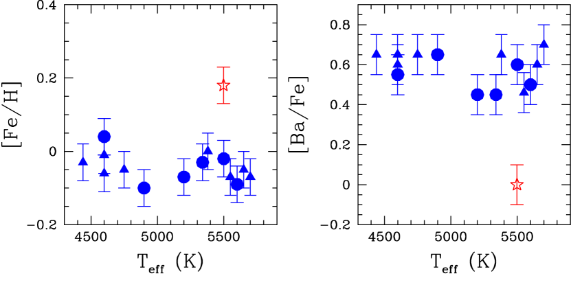
Figure 2: Fe and Ba abundances $versus$ effective temperatures for GJ 758 (starred symbol), the Argus association and the open cluster IC 2391 (triangles and circles, respectively, from De Silva et al. 2013).

Barium deserves a brief, separate discussion. Firstly identified by D’Orazi et al. (2009a), and subsequently confirmed by several studies (e.g., Yong et al. 2012; Jacobson & Friel 2013; Mishenina et al. 2013), the Ba abundance shows a decreasing trend with the open cluster’s age. The younger the cluster, the higher its Ba content. The reason of such peculiar and unique pattern is still matter of debate: it has been suggested that the efficiency in the production of the s-process elements in low-mass AGB stars is higher than what is predicted form standard stellar evolution models and input physics has to be revised (D’Orazi et al. 2009b; Maiorca et al. 2012). However, subsequent investigations have shown that the picture might not be that straightforward. The fact that the Ba overabundance is not accompanied by a similar behaviour in other s-process elements (e.g., Y, La) makes unlikely this explanation. We refer the reader to D’Orazi et al. 2012 for a wider discussion of this topic. Regardless of the nature of the super-solar Ba content, [Ba/Fe] ratios range from extremely high values of approximately $\sim$0.6 dex for pre-main sequence clusters, such as e.g., IC 2602 and IC 2391 (D’Orazi & Randich 2009) to solar values, or even lower, for clusters a few Gyr old. De Silva et al. (2013) corroborated this observational evidence and obtained a mean abundance of ${\rm[Ba/Fe]}=0.53\pm 0.03$ (rms=0.08 dex) for the Argus association and ${\rm[Ba/Fe]}=0.62\pm 0.02$ (rms=0.07) for IC 2391 (see the right-hand panel of Fig. 2). Conversely, we gathered a ${\rm[Ba/Fe]}=0.00\pm 0.12$ for our star, which implies a difference in the Ba content more than a factor of 3.5. Thus, in terms of chemical composition, Ba provides us with the strongest observational constraint: GJ 758 cannot be born from the same molecular cloud as Argus.

4.3 Age indicators

GJ 758 is known to have a low activity level as resulting from several measurements in the literature: $\log R_{HK}=-4.94$ (Wright et al. 2004), -5.015 (Isaacson & Fischer 2010); -5.060 (Duncan et al. 1991; Mamajek & Hillenbrand 2008). The calibration by Mamajek & Hillenbrand (2008) yields values of 5.5-7.7 Gyr for these activity values. The availability of multi-epoch measurements of chromospheric activity spanning several years indicate that this is not the result of a poor sampling of an activity cycle. The X-ray non-detection in the ROSAT All Sky Survey (Voges et al. 1999, 2000) (which would imply $\log L_{X}/L_{bol}<-5.8$ and then an age ¿ 3 Gyr), the small projected rotational velocity (0–2 km/s) and the small photometric variability (0.008 mag from Hipparcos) further support the low activity level of GJ 758, as expected for a few-Gyr old star.

Lithium is another highly-sensitive age indicator for young stars. From the analysis of the spectrum described in Sect. 4.2 the Li 6708Å  resonance line is not detected, confirming the null result by Takeda & Kawanomoto (2005). For stars with GJ 758 colors, detectable amounts of lithium vanish at about the age of the Hyades. Therefore, the lack of lithium allows us to infer a stellar age older than 600 Myr.

While stellar members of young moving groups display significant scatter in the age indicators (see Desidera et al. 2011, for the case of Argus), we are not aware of late G-type stars which are confirmed members of young moving groups which have such a low activity level and lack of lithium. The analysis of these indicators therefore converges with the chemical tagging in ruling out Argus membership for GJ 758.

Using the spectroscopic effective temperature and metallicity, and the Hipparcos $V$ magnitude and trigonometric parallax, we derive age and masses from isochrone using the PARAM interface (da Silva et al. 2006) and the stellar models by Bressan et al. (2012). Limiting possible input values to age larger than 0.6 Gyr, as resulting from the lack of lithium, the resulting age is $2.2\pm 1.4$ Gyr and the stellar mass $0.97\pm 0.02$ $M_{\odot}$.

4.4 Summary

All age indicators indicate that GJ 758 is an old star, with lithium providing a tight lower limit at 600 Myr. Chemical tagging derived from an homogeneous comparison of abundances of several elements with those of confirmed members of Argus association and IC 2391 open cluster also rules out a link between GJ 758 and Argus, with Barium abundance suggesting an age similar to the Sun. Therefore, we conclude that the kinematic parameters of GJ 758 are similar to those of Argus association just by chance, confirming the statistical nature of kinematic ages and the need for independent youth indications to conclusively infer membership in young moving groups (Gagné et al. 2014; Desidera et al. 2015). The young-disk kinematics decrease the probability of a star significantly older than the Sun. The age of the system is likely within 1 to 6 Gyr, and the most probable value around 3 Gyr, with isochrone fitting yielding younger values than chromospheric activity. We also confirm the moderate super-solar metallicity of the star.

5 Spectro-photometric analysis

The new SPHERE photometry is complementary to the existing set of photometric data points on the spectral energy distribution (SED) of the companion obtained by Janson et al. (2011). In the following we use the more complete SED to refine the properties of GJ 758 B.

5.1 Fluxes and magnitudes

We retrieved the apparent fluxes corresponding to the SPHERE/IRDIS photometry of the companion using the contrast ratio listed in Table 4 and following a three-steps process:

• We first built the 0.4-22.1 $\mu$m SED of the star from the Tycho $B_{T}$, $V_{T}$ (Hoeg et al. 1997), USNO-B $R$, and $I$ (Monet et al. 2003), and WISE W3-W4 photometry (Cutri & et al. 2013). The 2MASS $J$, $H$, $K_{s}$ (Cutri et al. 2003) and W1-W2 photometry could not be used because of the saturation of the star (see Janson et al. 2011). The optical photometry was converted to apparent fluxes using the Gemini flux-conversion tool. We considered the WISE zero points reported in Jarrett et al. (2011) for the infrared part.

• We adjusted a GAIA-COND model (Brott & Hauschildt 2005) with $T_{e\!f\!f}=5400$ K, $\log\leavevmode\nobreak\ g=4.0$ dex, and ${\rm M/H}=0.0$ onto GJ 758 A fluxes values. This model has atmospheric parameters close to the ones determined from high-resolution spectra of the star ($T_{e\!f\!f}=5435$ K, $\log\leavevmode\nobreak\ g=4.0$, ${\rm M/H}=0.12$; Kovtyukh et al. 2004). The GAIA model reproduces well the SED of GJ 758 (Fig. 3), including the 2MASS $K_{s}$ band photometry, which appears to be less affected by the saturation.

• We derived the mean stellar flux into the SPHERE/IRDIS passbands using the flux-calibrated GAIA spectrum, and the tabulated filter widths reported in Table 1.

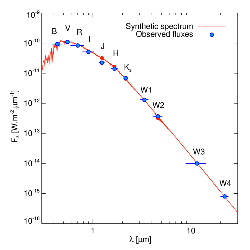
Figure 3: GAIA-COND synthetic spectrum adjusted onto the spectral energy distribution of GJ 758 A built from a compilation of optical, near-infrared, and mid-infrared photometry. The 2MASS J, H, K_s and WISE W1-W2 photometry data were excluded from the fit because the star was saturating in the 2MASS images.

The remaining fluxes of GJ 758 B were estimated directly from a flux-calibrated spectrum of Vega (Bohlin 2007), the Keck/NIRC2 and Gemini/NIRI magnitudes of the companions reported in Janson et al. (2011), and corresponding filter transmission curves. The effect of the telluric absorption on the final flux estimates for the companion was simulated using the ESO sky model calculator (Noll et al. 2012; Jones et al. 2013). We considered two altitudes of targets above the horizon (90 and 30^∘) to simulate dry and wet conditions. The effect is found to be negligible compared to the error on the companion photometry. The final estimated fluxes of GJ 758 B considered for the following analysis are reported in Table 6. The fluxes in the overlapping narrow-band K1 and $K_{c}$ filters are almost identical. This is an indication that our flux-conversion methods yield consistent results.

Table 6: Apparent fluxes of GJ 758 B.

Filter	$\lambda$	$\Delta\lambda$	$F_{\lambda}$	$\Delta F_{\lambda}$	Ref
	(nm)	(nm)	(W.m${}^{-2}.\mu$m-1)	(W.m${}^{-2}.\mu$m-1)
Y2	1022	51	5.074$\times 10^{-17}$	9.703$\times 10^{-18}$	1
Y3	1076	54	8.526$\times 10^{-17}$	7.368$\times 10^{-18}$	1
J2	1190	48	3.449$\times 10^{-17}$	8.532$\times 10^{-18}$	1
J	1250	180	1.126$\times 10^{-16}$	2.280$\times 10^{-17}$	2
J3	1273	51	2.070$\times 10^{-16}$	3.508$\times 10^{-17}$	1
CH4S	1580	103	4.074$\times 10^{-17}$	8.240$\times 10^{-18}$	2
H2	1593	53	1.177$\times 10^{-16}$	1.255$\times 10^{-17}$	1
H	1650	290	2.536$\times 10^{-17}$	5.130$\times 10^{-18}$	2
H3	1667	56	1.222$\times 10^{-17}$	5.605$\times 10^{-18}$	1
CH4L	1690	110	$\leq$1.457$\times 10^{-17}$	…	2
$\mathrm{K_{c}}$	2098	28	2.747$\times 10^{-17}$	5.550$\times 10^{-18}$	2
K1	2110	105	2.897$\times 10^{-17}$	5.859$\times 10^{-18}$	1
K2	2251	112	1.145$\times 10^{-17}$	4.209$\times 10^{-18}$	1
L’	3776	700	2.163$\times 10^{-17}$	2.090$\times 10^{-18}$	2
$\mathrm{M_{s}}$	4670	241	$\leq$5.257$\times 10^{-17}$	…	2

(1) This work; (2) Janson et al. (2011).

Table 7: Absolute magnitudes of GJ 758 A, GJ 758 B, and of the candidate companion estimated from the contrast ratio and the model spectrum of the star.

Filter	GJ 758 A	GJ 758 B	New c.c.
Y2	$4.29\pm 0.03$	$19.19\pm 0.20$	$19.74\pm 0.62$
Y3	$4.23\pm 0.03$	$18.43\pm 0.10$	$18.73\pm 0.86$
J2	$4.09\pm 0.03$	$19.06\pm 0.25$	$18.76\pm 0.60$
J3	$3.94\pm 0.03$	$16.83\pm 0.18$	$18.95\pm 0.92$
H2	$3.64\pm 0.03$	$16.59\pm 0.12$	$18.31\pm 0.61$
H3	$3.59\pm 0.03$	$18.88\pm 0.42$	$18.23\pm 0.61$
K1	$3.58\pm 0.03$	$17.03\pm 0.21$	$17.35\pm 0.62$
K2	$3.57\pm 0.03$	$17.78\pm 0.35$	…

5.2 Comparison of GJ 758 B to empirical objects

The Y3/J2, J2/J3, H2/H3, and K1/K2 flux ratios provide a clear detection of water and methane absorptions around 1.15, 1.6, and 2.3 $\mu$m in the atmosphere of the brown-dwarf companion. We compared its 1–2.5 $\mu$m SED to those of 101 T0–T8 field dwarfs with near-infrared spectra taken from the SpeXPrism library (Burgasser 2014). The mean flux $F_{k,i}$ and error $\sigma_{F_{k,i}}$ associated to each template spectrum $k$ and filter passband $i$ was estimated and compared to the companion SED $f$ and error $\sigma_{f}$ using the $G^{\prime\prime}$ goodness-of-fit indicator defined by Bowler et al. (2010):

$$G^{\prime\prime}_{k}=\sum_{i=1}^{n}w_{i}\frac{(f_{i}-C^{\prime\prime}_{k}F_{k,i})^{2}}{\sigma_{f_{i}}^{2}+(C^{\prime\prime}_{k}\sigma_{F_{k,i}})^{2}}$$ (1)

where $C^{\prime\prime}_{k}$ is a renormalization factor applied to the template SED $k$ which minimizes $G^{\prime\prime}_{k}$. $w_{i}$ is the renormalized FWHM $\Delta\lambda_{i}$ of each filter $i$ following:

$$w_{i}=\frac{\Delta\lambda_{i}}{\sum_{j=1}^{n}\Delta\lambda_{j}}$$ (2)

The indicator enables us to compare SEDs with an inhomogeneous wavelengths sampling and with measurement errors on both the templates and the object. We rejected solutions which exceeded the upper limit of the flux into the CH4L passband (Janson et al. 2011). The $G^{\prime\prime}$ indicator is minimized for the T6.5 dwarf 2MASS J22282889-4310262 (Burgasser et al. 2004) which is known to experience wavelength-dependent photometric variability (Buenzli et al. 2012). The comparison is shown in the upper panel of Fig. 4, and we report the $G^{\prime\prime}$ values as a function of spectral type in Fig. 5. When flux-calibrated and scaled to the distance of GJ 758 B (using the parallax of Faherty et al. 2012), the spectrum of 2MASS J22282889-4310262 is over-luminous and a multiplication factor of 0.08 must be applied to fit the companion SED. This indicates that GJ 758 B is most likely later than T6.5. The variation of $G^{\prime\prime}$ with the spectral type also clearly confirms that the companion is later than T5. This is in agreement with the conclusions of Janson et al. (2011).

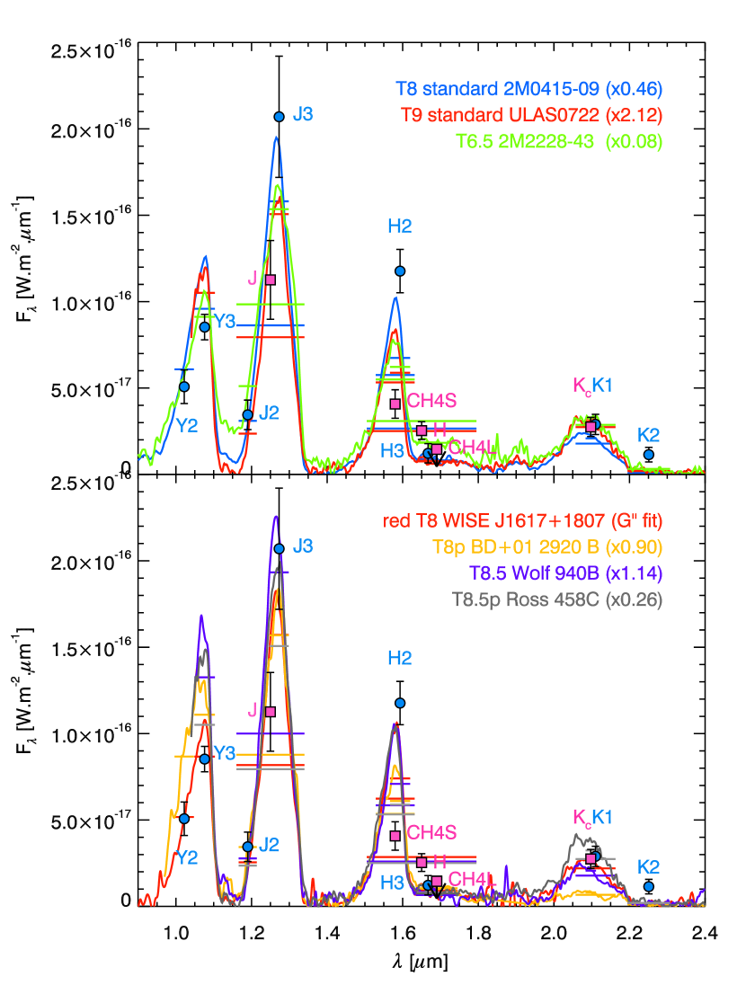
Figure 4: Comparison of the 1–2.5 $\mu$m spectral-energy distribution of GJ 758 B to those of T8, T9 standard, benchmark companions, and to the red T8 dwarf WISEJ1617+1807 (Burgasser et al. 2011). The large blue circles represent our new IRDIS measurements, while the large pink squares represent the measurements from Janson et al. (2011). The horizontal lines correspond to the expected fluxes of the empirical objets in each filter bandpass.

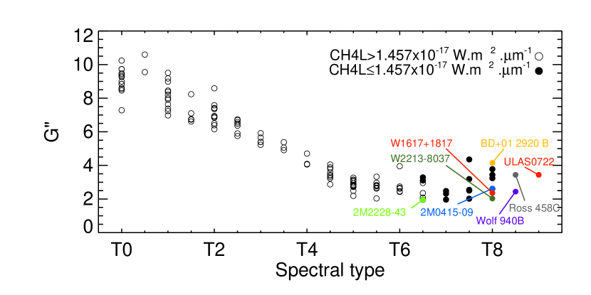
Figure 5: $G^{\prime\prime}$ values inferred from the comparison of SEDs of T dwarfs (generated from SpecXPrism spectra) with with GJ 578 B’s. The re-normalized SEDs whose flux in the CH4L passband respect the upper limit set for GJ 758 B are reported as filled dots. Those who don’t are reported with open circles. The G” values for the objects considered in Fig. 4 are overlaid. We also report the value for the red T8 dwarf WISEP J231336.41-803701.4 whose SED, along with the one of the red T8 WISEP J161705.75+180714.0 provide the best visual fits to the SED of the companion.

We show in the lower panel of Fig. 4 the spectra of standard T8 and T9 dwarfs (Burgasser et al. 2004; Lucas et al. 2010) with measured trigonometric parallaxes and fluxes brought to the distance of the GJ 758 system. The companion SED is midway between the renormalized SED of the T8 and T9 standards. Nevertheless, the templates fail to reproduce the J3, H2, and K2 fluxes simultaneously. The companion also appears to have a luminosity intermediate between these two objects. Its $J$ and $H$ band absolute magnitudes agree well with the mean values reported in Dupuy & Kraus (2013) for T8-T8.5 objects.

The causes of the peculiar SED of GJ 758 B are unclear. The companion spectrophotometric properties could be related to a non-solar composition, or a surface gravity different than those of the standard T8-T9 dwarfs. Both parameters produce opposite effects on 1–5 $\mu$m SEDs that are difficult to disentangle (e.g. Leggett et al. 2010). We used the spectra of wide companions to stars with known age, and metallicity to investigate the effect of peculiar atmospheric parameters, making the assumption that these objects share the same composition as their host star.

Ross 458 C (Goldman et al. 2010; Scholz 2010) appears as the only object with an estimated age (150–800 Myr) younger than the typical field dwarf ages ($\gg$500 Myr) which has an estimated $T_{e\!f\!f}$ (625-755 K Burgasser et al. 2010; Burningham et al. 2011) and near-infrared spectral type (T8.5p) in the same range as that of GJ 758 B (Janson et al. 2011). It is also reported to have a super-solar metallicity (Fe/H = +0.2–0.3; Burgasser et al. 2010), e.g. similar to that of GJ 758 A (+0.2 dex, see Sect. 4). The spectra of both objects are also compared in the lower panel of Fig. 4. The spectrum of Ross 458 C from Burningham et al. (2011) represents the SED of GJ 758 B less well than the T8 standard. Its enhanced flux at $K$-band suggests that the two companions do not span the same surface gravity and/or metallicity interval.

We considered the opposite case of the peculiar T8 companion to the metal-poor (${\rm[Fe/H]}=-0.38\pm 0.06$ dex) G-type star BD+01 292 (Pinfield et al. 2012) and of the T8 companion to the sdM1.5+WD binary Wolf 1130 (${\rm[Fe/H]}=-0.64\pm 0.17$). Both companions have a suppressed flux at $K$-band, possibly due to the enhanced collision-induced absorption of H₂ encountered into clear/low-metallicity/higher-pressure atmospheres (Saumon et al. 1994; Borysow et al. 1997). They clearly produce a worse fit to the SED of GJ 758 B than the T8 standard does. In summary, we see an opposite trend for GJ 758 B departure from the SED of the standard T8.

The T8.5 companion to the old (3.5–6 Gyr) solar-metallicity star Wolf 940 (Burningham et al. 2009, ${\rm[Fe/H]}=-0.06\pm 0.20$) represents the $J$ band flux better, at the price of a degradation of the fit in the $Y$ band. We do not find a good fit with earlier type companions such as GJ 229 B (T7pec) or Gl 570 D (T7.5) (Geballe et al. 1996, 2001) and primaries with roughly solar-metallicities (Neves et al. 2014).

We extended the comparison to additional peculiar dwarfs with red near-IR colors but no a priori knowledge of their age and metallicity (e.g. Mace et al. 2013, and references therein). We find that the red T8 dwarfs WISEP J161705.75+180714.0 and WISEP J231336.41-803701.4 (Burgasser et al. 2011) provide the best fit among all other aforementioned objects. They notably represent the $Y$ band flux well compared to the other objects. Burgasser et al. (2011) note that the spectral properties of these two objects suggest cool ($T_{e\!f\!f}=600$ K), low surface gravity ($\log\leavevmode\nobreak\ g=4.0$), and cloudy atmospheres.

In summary, we cannot find an empirical object with known metallicity and distance that accurately represents all the near-IR narrow-band and broad-band fluxes of GJ 758 B simultaneously. We estimate a T8 spectral type from this comparison. The analysis is however certainly limited by the small amount of spectra of T8–T9 dwarfs with robust constraints on their age and metallicity.

5.3 Comparison of GJ 758 B to atmospheric models

We compared the SED of GJ 758 B to four sets of atmospheric models – BT-Settl, Exo-REM, Morley+12 and Saumon+12 – in order to refine the estimate of $\log\leavevmode\nobreak\ g$, $T_{e\!f\!f}$, and Fe/H, and to understand its peculiar photometry. The models are described in Allard et al. (2013), Baudino, J.L. et al. (2015), Morley et al. (2012), and Saumon et al. (2012) respectively. The specificities and parameter space of the models are decribed in more details in Appendix A and Table 11. We expect that the use of these different classes of models allows the best possible approach for the accurate modeling of the atmospheric parameters.

In order to account for the inhomogeneous sampling of the real SED during the fitting process, we decided to use the goodness-of-fit $G_{k}$ indicator defined by Cushing et al. (2008). This indicator contains a dilution factor, $C_{k}$, similar to the $C^{\prime\prime}_{k}$ factor defined in Eq. 1. $C_{k}$ usually equals $(R/d)^{2}$, where $d$ is the distance of the source and $R$ its radius. Given the Hipparcos distance of GJ 758 A, we were able to retrieve the optimal average object radii for each given model.

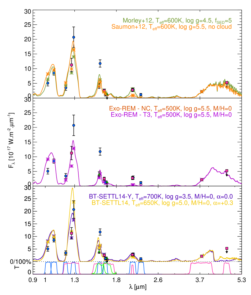
Figure 6: Comparison of the 1-5 $\mu$m spectral-energy distribution of GJ 758 B to the best fitting synthetic spectra from the BT-SETTL14, Morley+12, Saumon+12, and Exo-REM grids. The asterisks represent the fluxes in each bandpass expected from the atmospheric models. The Exo-REM and Exo-REM - NC models completely overlap because at this combination of $T_{e\!f\!f}$ and $\log\leavevmode\nobreak\ g$, the cloud condensation occurs below the considered pressure grid, effectively making both models cloud-free.

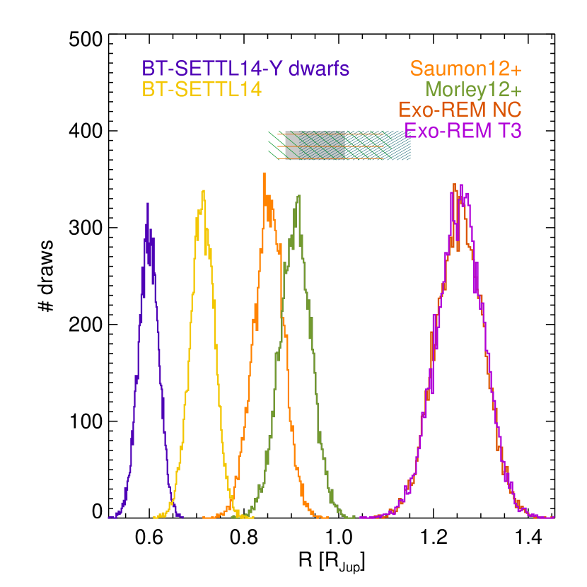
Figure 7: Histogram of radii (dilution factors $C_{k}$, directly related to radius because the distance is known) derived from the comparison of the most frequent best-fitting solution for each Monte-Carlo simulation of the SED of GJ 758 B. The hatched areas correspond to the range of radii predicted for the estimated $T_{e\!f\!f}$ and age of the system by the Saumon & Marley (2008) models with cloudy (blue hatches), hybrid clouds (red hatches), and cloudless (green hatches; covering $[{\rm M/H}]$ of 0, 0.3, and -0.3 dex) atmospheres considered as boundary conditions. The shaded zone correspond to the predictions of the COND models (Baraffe et al. 2003).

Confidence levels cannot be derived directly from $G$. Therefore, we followed the approach of Cushing et al. (2008) to determine the most meaningful fitting solution of each model grid. For each photometric data point of the object, we generated a normal Monte-Carlo (MC) distribution of 10 000 draws with mean values of $f_{i}$ and standard deviations of $\sigma_{i}$. The $G_{k}$ values were computed for each of the resulting 10 000 SEDs. We computed for each models of the grid, the fraction of the 10 000 MC simulated SEDs that were best fitted by this given model. This $f_{MC}$ indicator, ranging from 0 to 1, enables to test the significance of any fitting solution. The models with the highest $f_{MC}$ value represents the most significant solution. However, we note that $f_{MC}$ is sensitive to the sampling and extent of the model grid. Therefore, despite the criterion is usefull to estimate the robustness of a given solution within a grid, it should not be used to evaluate the quality of the solutions found with different grids. We performed a visual inspection of the three solutions with the highest $f_{MC}$ for each model grid, but only reported the atmospheric parameters and $f_{MC}$ of the most probable solution in Table 8.

The Monte-Carlo method works as long as the errors associated to $f_{i}$ are uncorrelated. In the case of GJ 758 B, the errors associated to the flux-calibrated SED of the object combine uncorrelated errors corresponding to the companion contrast values associated to each filter to a correlated error arising for the flux-calibrated spectrum of the star. We accounted for both sources of errors in our MC simulations by multiplying the 10 000 MC SEDs of the companion by $10^{-0.4\times\textsl{N}(\mu=0,\sigma_{ph})}$ with N an additional MC normal distribution of 10 000 values with mean values of 0 and standard deviation $\sigma_{ph}$ equal to the magnitude error on the flux scaling of the companion spectrum. We took $\sigma_{ph}=0.03$ mag, which corresponds to the highest photometric error on the SED of the star.

The results of the fits are reported into Table 8 and shown in Fig. 6. The solutions with the highest $f_{MC}$ always correspond to the solution with the minimum $G$. The corresponding dilution factors inferred from our MC simulations for the most probable fitting solution (highest $f_{MC}$) are shown in Fig. 7. No one model represents well the whole SED, especially the J3 and H2 fluxes. The Morley+12 models provide the best fits according to the $G$ indicator. The three most significant solutions ($>$65% of the solutions) found with these models correspond to log g=4.0-4.5 and $T_{e\!f\!f}=550-600$ K. The cloud-free Saumon+12 models only provides a better fit to the $J$ band flux. But their poorer representation of the other bands indicate that clouds are still needed in the photosphere to reproduce the GJ 758 B SED. Visually, the BT-SETTL14 models seem to provide a better fit to the $H$ band flux. The flux drop at $M_{s}$ band in the BT-SETTL14 models is in better agreement with the upper limit found by Janson et al. (2011). New deeper observations at $M$ band of the GJ 758 system could help to further discriminate the models. The BT-SETTL14 models do not provide any meaningful constraints on the log g. A re-analysis with a classical $\chi^{2}$ confirms the conclusions. The radii (dilution factors) needed to adjust the surface flux predicted by the models onto the apparent flux of the companion are unphysical in the case of the BT-SETTL14 models. This may indicate that the $T_{e\!f\!f}$ of GJ 758 could be lower than the one corresponding to the best fit. The Exo-REM models fail to represent correctly the SED of the companion, especially in the $Y$, $H$, and $K$-bands.

We conclude that the companion has $T_{e\!f\!f}=600\pm 100$ K from the above analysis. This is in good agreement with Janson et al. (2011) whose analysis relied on the models of Burrows et al. (2006) extended to colder temperatures (Hubeny & Burrows, in prep.). The Morley+12 parametric model points toward a low surface gravity, in agreement with the hints found in Sect. 5.2. But the inexistent exploration of the effect of the metal-enrichment in these grids of models associated to model uncertainties certainly biases the analysis. A low-resolution spectrum of the source would be needed to determine with good confidence $\log\leavevmode\nobreak\ g$ and M/H.

From the $T_{e\!f\!f}$ and the derived age for the system ($3^{+3}_{-2}$ Gyr, see Sect. 4), we estimate a mass of $23^{+17}_{-13}$ $M_{\mathrm{Jup}}$ for GJ 758 B using the BT-SETTL13 grid of models (Allard et al. 2013). This value is in the low range of the masses inferred by Janson et al. (2011), as a direct consequence of our estimated age range for the system that is slightly younger than the one they considered.

Finally, we report in Table 9 the predictions from the Baraffe et al. (2003) and Saumon & Marley (2008) models. The models predict radii corresponding to the estimate $T_{e\!f\!f}$ in the range 0.80–1.21 $R_{Jup}$ which are marginally consistent with the radii derived from the SED fit with the Exo-REM, Saumon12+ and Morley12+ models. They are still 25 and 11% larger than those infered from the SED fit with the BT-SETTL14-Y dwarfs and BT-SETTL14 models respectively (see Fig. 7). The difference may arise from the different boundary conditions considered for the evolutionary models and the atmospheric models used for the SED fit. Nevertheless, it is more likely that the $T_{e\!f\!f}$ derived from the SED fit is slightly overestimated by the SETTL models (by 100–200 K) and lead to this inconsistency.

Table 8: Fitting solutions with the highest $f_{MC}$ values for the GJ 758 B SED and the three sets of atmospheric models using the $G$ goodness-of-fit indicator.

Model	$T_{e\!f\!f}$	$\log\leavevmode\nobreak\ g$	[M/H]	$[\alpha]$	$f_{SED}$	R	G	$f_{MC}$
BT-SETTL14-Y	700	3.5	0.0	0.0	n/a	0.60	1.80	0.55
BT-SETTL14	650	5.0	0.0	0.3	n/a	0.71	1.60	0.20
Exo-REM - NC	500	5.5	0.0	0.0	n/a	1.26	4.83	0.85
Exo-REM - T3	500	5.5	0.0	0.0	n/a	1.26	4.83	0.63
Morley+12	600	4.5	0.0	0.0	5.0	0.91	1.39	0.30
Saumon+12	600	5.5	0.0	0.0	n/a	0.85	2.70	0.74

Table 9: $T_{e\!f\!f}$ and radius predictions from the Baraffe et al. (2003) and Saumon & Marley (2008) models

Models	Boundary	M/H	$R$	Mass
		(dex)	($R_{\mathrm{Jup}}$)	($M_{\mathrm{Jup}}$)
Saumon+08	No cloud	0	$0.96^{0.14}_{0.10}$	$24^{+16}_{-13}$
Saumon+08	No cloud	$+$0.3	$0.97^{0.15}_{0.10}$	$24^{+15}_{-14}$
Saumon+08	No cloud	$-$0.3	$0.95^{0.15}_{0.10}$	$24^{+16}_{-13}$
Saumon+08	Cloudy	0.0	$1.01^{0.15}_{0.10}$	$21^{+14}_{-11}$
Saumon+08	Hybrid	0.0	$0.96^{0.13}_{0.10}$	$24^{+14}_{-13}$
COND	AMES-COND	0.0	$0.97^{0.05}_{0.08}$	$21^{+11}_{-10}$

5.4 Nature of the new candidate companion

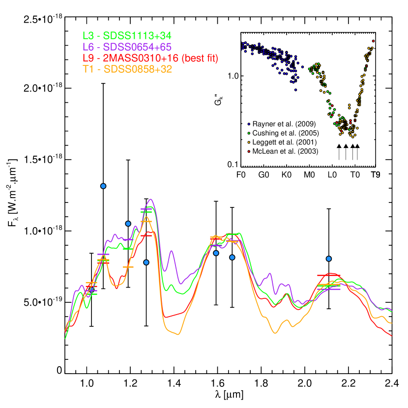
Figure 8: Comparison of the flux of the newly identified candidate (blue circles) with SEDs of different sub-stellar objects of spectral types L3, L6, L9 (best fit) and T1. For each spectral type, we plot the object that provides the best fit according to the $G^{\prime\prime}_{k}$ indicator. The inset plot at the top shows the $G^{\prime\prime}_{k}$ values as a function of spectral type for $\sim$400 objects taken from various libraries (Leggett et al. 2001; McLean et al. 2003; Cushing et al. 2005; Rayner et al. 2009). The vertical arrows indicate the spectral type of the plotted SEDs.

The detection of a new candidate companion around a star with an already known companion is particularly interesting. It is going to become very common with the new generation of high-contrast imagers because of the boost in sensitivity that they provide at smaller angular separations. For the new candidate detected in our IRDIS data, we make use of the large multi-wavelength coverage ($Y$- to $K$-band) to perform a photometric analysis.

Although the error bars on the photometry of the new candidate are large (¿0.5 mag, see Table 7), we attempt a first-order estimation of its spectral type by comparing its observed flux with the SEDs of stellar and sub-stellar objects. The star data are taken from the IRTF stellar library (Cushing et al. 2005; Rayner et al. 2009), while the brown dwarf data are taken from the NIRSPEC brown dwarf spectroscopic survey (McLean et al. 2003) and from Leggett et al. (2001). For the comparison, we use the $G^{\prime\prime}_{k}$ indicator as in Sect. 5.2. The results are presented in Fig. 8, where we show the $G^{\prime\prime}_{k}$ values as a function of spectral types (inset), and the SEDs of four objects that can fit equally well the photometry of the new candidate within the error bars.

The $G^{\prime\prime}_{k}$ distribution shows a rather flat minimum in the L3–T1 range, indicating that our candidate could likely be of sub-stellar nature. However, reaching a final conclusion is difficult from our current data because of the significant uncertainties on the photometry. As showed in Fig. 8, the candidate photometry is compatible with mid-L to early-T types, but late-M and early-L (not showed) would also provide decent fit. We note that the low galactic latitude of GJ 758 (+8 deg) increases significantly the probability of background contamination, particularly with late M stars, which are the main source of contamination at high-contrast (e.g. Chauvin et al. 2015).

Other possibilities for the nature of the candidate could include Solar System bodies, such as asteroid and trans-neptunian objects, or extra-galactic objects. However, an asteroid basically reflects the near-IR light from the Sun, resulting in a very flat G2V spectrum that is not compatible with the photometry. In addition, these objects would be characterized by a very large proper motion of several mas to several dozens of mas per second. Our observations taken over two consecutive nights completely rule out this possibility. On the other hand, extra-galactic sources such as galaxies are another possibility, but they would be resolved even at significant redshifts by the very fine plate scale of IRDIS ($\sim$12.25 mas, see Table 3). The point-like structure of the candidate also rules out this possibility.

In conclusion, we cannot rule out the possibility that the new companion is indeed bound to GJ 758, since its photometry is broadly compatible with L-type objects. A second epoch will be required to clear any possible doubt. Given the high proper motion of the star ($\sim$180 mas/yr), a confirmation of the status of this candidate is already possible.

6 Astrometry and orbital properties

6.1 Least-Square Monte Carlo orbital fitting

(a)

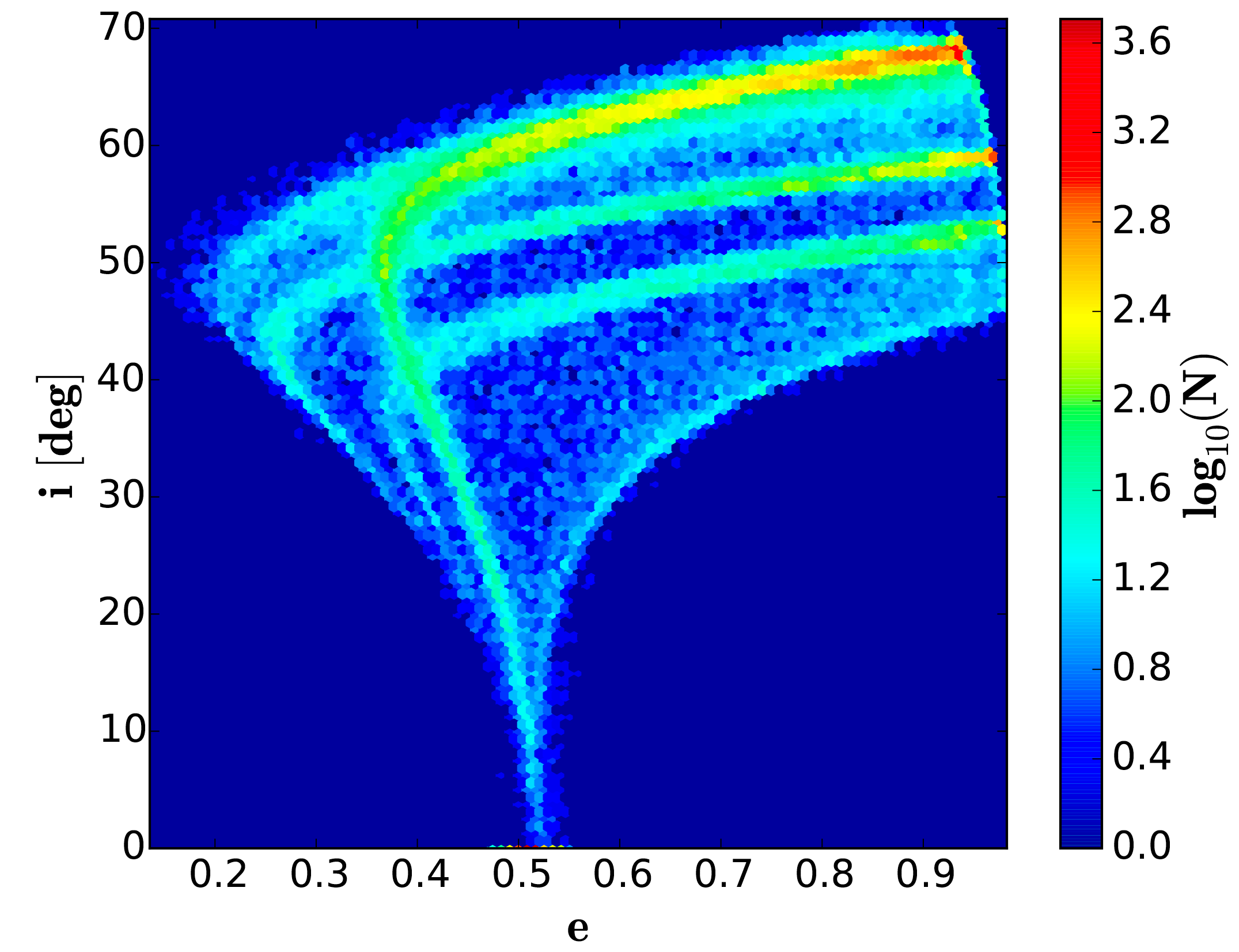
(b)

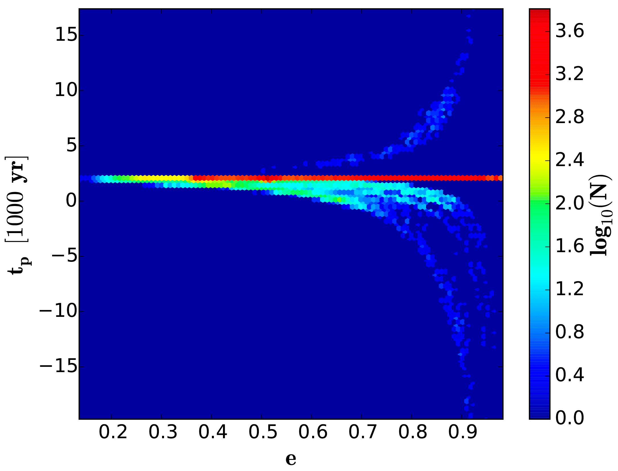
(c)

Figure 9: Semi-major axis, inclination and time of periastron passage as function of eccentricity for all solutions with $\chi^{2}_{red}\ \leq\ 2$ out of 5 000 000 runs of our LSMC fit. Logarithmic density of solutions is indicated by color.

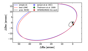
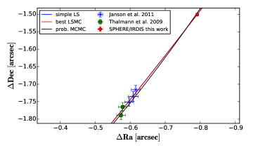
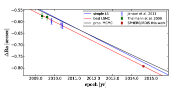
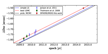
Figure 10: Best fitting orbits recovered with simple least squares fitting as well as LSMC fitting. In addition, we show a probable orbit with orbital elements close to the peak values recovered by our MCMC fit (see Sect. 6.2). Solid lines represent the apparent orbits. The corresponding orbital elements are listed in Table 10. We show the data points taken with Subaru/HiCIAO (green squares) as given in Thalmann et al. (2009), as well as the data points taken with Subaru/HiCIAO, Gemini/NIRI and Keck/NIRC2 (blue crosses) given in Janson et al. (2011) together with our SPHERE/IRDIS measurement (red circle).

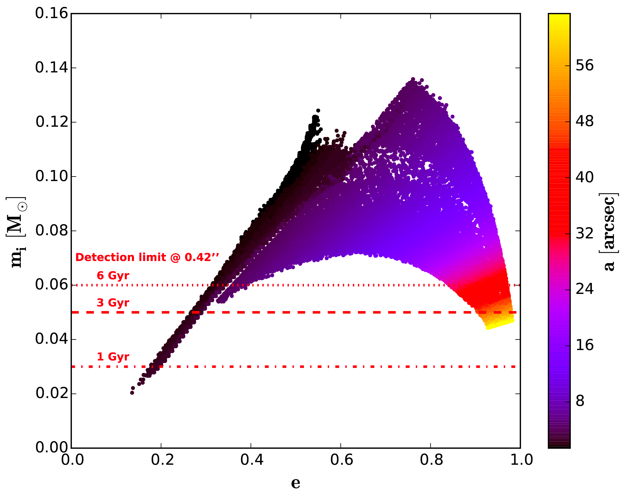
Figure 11: Minimum mass of an unseen inner companion that would cause a false positive eccentricity signal in the relative astrometry of GJ 758 A and B by astrometric displacement of GJ 758 A due to their common orbit around the center of mass of the system. The minimum mass is a function of the eccentricity and semi-major axis of the A/B system as well as the maximum epoch difference of all astrometric measurements. Shown are such minimum masses for all orbits with $\chi^{2}_{red}\ \leq\ 2$ which were recovered for the A/B system. Using our deep SPHERE/IRDIS observations as well as the AMES-COND models Baraffe et al. (2003) we also show the detectable minimum mass at the angular separation at which such a putative inner companion would need to reside. We can exclude the presence of an object that would introduce a false positive eccentricity in all cases.

We used the new IRDIS astrometric measurement to put constraints on the orbital solution of the system. In previous studies by Thalmann et al. (2009) and Janson et al. (2011), it was already shown that the system presents significant orbital motion and Monte-Carlo simulations were used to get a first estimate of the orbital elements. In this study we used first a Least-Squares Monte-Carlo (LSMC) approach to study the parameter space of possible orbits. For this purpose we created $5\times 10^{6}$ sets of orbital elements, which were drawn from uniform distributions. These sets of orbital elements were then used as starting points for a least-squares minimization routine. The method is described in detail in Ginski et al. (2013). To limit the parameter space we fixed the total mass of the system to the nominal value of $\sim$1 $M_{\odot}$: 0.97 $M_{\odot}$ for the star (Takeda et al. 2007) and $\sim$0.03 $M_{\odot}$ for the companion at the probable age of the system. In addition, we limited the semi-major axis to values smaller than 63.45″(1000 AU at a distance of 15.76 pc). This is assuming that the system is long-term stable against disruption in the galactic disk as described in Close et al. (2003). Given the high age of the system ($3^{+3}_{-2}$ Gyr, see Sect. 4) and the fact that we still find the companion close to the host star, this assumption seems reasonable.

The results of our simulations are shown in Fig. 9. We do not show the results for the longitude of the ascending node and the argument of the periastron, since they are not well constrained yet by the available astrometry. In Fig. 10 we show the best fitting orbit solution that was recovered by the LSMC orbit fit. The corresponding orbital elements are shown in Table 10 alongside with the results recovered by our Markov-Chain Monte-Carlo simulation discussed in the following section.

Since the orbit does not show significant curvature yet, we cannot put an upper limit to the semi-major axis or the eccentricity. However, we find a lower limit of 0.14 for the eccentricity and 21.9 AU (1.39″) for the semi-major axis. In general, the semi-major axis of possible orbits scales with the eccentricity as can be seen in Fig. 9a. The minimum values of the semi-major axis and the eccentricity, as well as the general behavior of the well fitting orbit solutions, is consistent with the results presented in Janson et al. (2011), which were derived from simple Monte-Carlo simulations.

In Fig. 9b we show the inclination of possible orbital solutions as function of eccentricity. For close to face-on orbits (inclination close to 0 deg) we can constrain the eccentricity of the orbit to values between 0.47 and 0.55. This range becomes continuously larger with increasing orbit inclination. For an inclination of $\sim$50 deg, the full range of recovered eccentricities gives results consistent with the astrometric measurements. We can put an upper limit on the inclination of 70.8 deg, i.e. we can exclude edge-on orbit solutions. If we compute a simple median of the recovered orbit inclinations we get a value of $58.9\pm 18.8$ deg. This is, within the given uncertainties, consistent with the interval found in Janson et al. (2011). Inclinations smaller than 40 deg correspond to small semi-major axes, with an upper limit of 77.5 AU (4.92″), while for larger values of the inclination, orbit solutions with the full range of recovered semi-major axes are possible.

Finally, in Fig. 9c we show the times of the periastron passage that we recovered from our simulations. The vast majority (87.5%) of our solutions passes the periastron between the years 2000 and 2065. The solutions that show the periastron passage at the time of the observations are generally highly eccentric and have large semi-major axes, which would explain that no curvature of the orbit is observed yet.

While these solutions fit the orbit very well geometrically, they are, however, very unlikely, given that the companion would spend the vast majority of the time at much larger separations from the primary star than where it was discovered. Indeed if we use the orbital period of roughly 26000 yr of the best fitting LSMC orbit we can estimate that the probability to find the companion within 30 years of the periastron passage is only on the order of 0.1 %. However, the orbits that pass the periastron within the next few decades can have lower eccentricities and semi-major axes. For an eccentricity around $\sim$0.5 there is a strong peak for the time of the periastron passage in the year 2040. It will thus be increasingly interesting to continue an astrometric monitoring of this system, since significant acceleration (i.e. curvature of the orbit) would be expected especially for cases with non-extreme eccentricities.

Since it is of specific interest if the system might indeed exhibit a high eccentricity (i.e. for plausibility of scattering scenarios during its early formation), we examined how reliable the eccentricities of our recovered orbit solutions are. Pearce et al. (2014) studied the possibility that an unknown inner (sub)stellar companion could introduce a false-positive eccentricity signal in the relative astrometry between the primary star and the known directly imaged companion. This is due to the astrometric displacement of the primary star as it orbits around the common center of mass with the hypothetical inner companion. We used their formalism to calculate the mass and angular distance that would be required for such an inner companion to make the orbit solution for GJ 758 B appear eccentric when the real orbit is in fact circular. We did this for all the orbit solutions that fit the astrometric measurements, and the results are shown in Fig. 11. We find that such a hypothetical inner companion would need masses between 0.02 $M_{\odot}$ and 0.14 $M_{\odot}$ with an orbit separation of 0.42″(6.6 AU; dependent on the mass of the system and the epoch difference of the astrometric observations). For the large majority of our solutions, we can reject such a companion because it would have been discovered in our deep IRDIS images (see Sect. 7 for detection limits estimations). However, due to the old age of the system, we would have not been able to recover inner companions with masses below $\sim$0.05 $M_{\odot}$ at the required angular separation.

To exclude the remaining possible solutions, we retrieved archival radial velocity data of GJ 758 A obtained with the ELODIE high-precision fiber-fed echelle spectrograph (Baranne et al. 1979) covering a time baseline of 7.8 years, as well as archival data from the Lick Planet Search program covering 13.2 years (Fischer et al. 2014). This combined data, showed in Fig. 12, covers a total of 16 years. It can be used to reject any hypothetical companion on a 17 years period more massive than 0.02 $M_{\odot}$ having any inclination higher than 5 degrees. Given the spherical symmetry of the system, this translates into a rejection of 98% of the orbital solutions for a hypothetical 0.02 $M_{\odot}$ inner companion and an increasing rejection rate for higher masses. It is thus extremely unlikely that the observed eccentricity is due to an inner companion causing an astrometric signal.

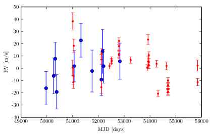
Figure 12: Radial velocity measurements of GJ 758 A, retrieved from the ELODIE (large blue dots) and Lick Planet Search (small red dots) archives. The measurements cover a total of 16 years which is nearly the full period of the inner companion speculated from the astrometric signal.

6.2 Markov-Chain Monte-Carlo orbital fitting

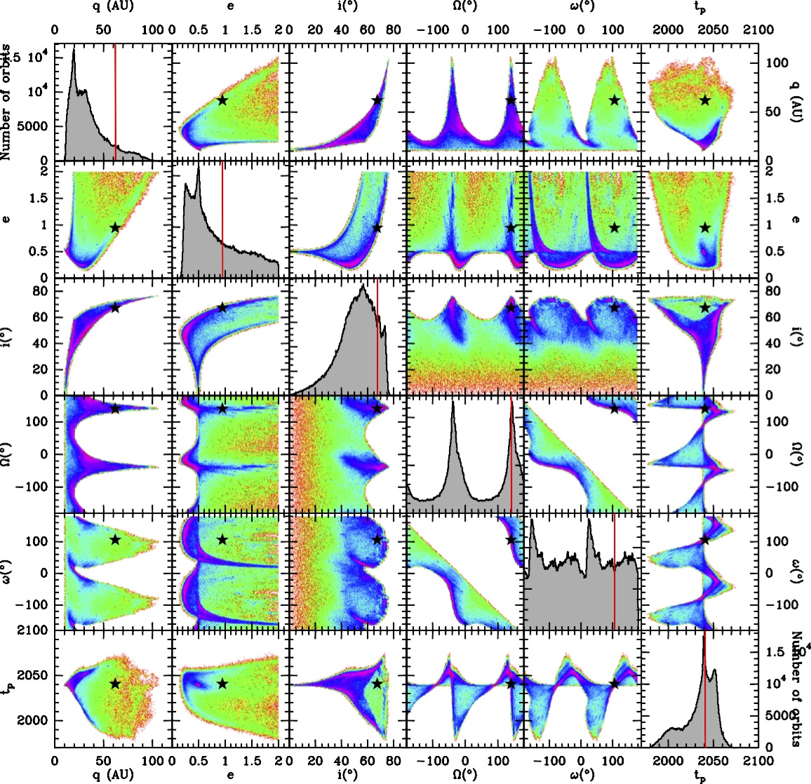
Figure 13: Resulting MCMC posterior distribution of the six orbital elements ($q$, $e$, $i$, $\Omega$, $\omega$, $t_{p}$) of GJ 758 B’s orbit using the universal variable code. The diagonal diagrams show mono-dimensional probability distributions of the individual elements. The off-diagonal plots show bidimensional probability maps for the various couples of parameters. This illustrates the correlation between orbital elements. The logarithmic color scale in these plots is linked to the relative local density of orbital solutions. It is indicated on the side of Fig. 14. In the diagonal histograms, the red bar indicates the location of the best $\chi^{2}$ solution obtained via standard least-square fitting. The location of this solution is marked with black stars in the off-diagonal plots. This solution is also plotted in Fig 10.

Table 10: Orbital characteristics of the best $\chi^{2}$ solution recovered by simple least-squares fitting (first column), as well as LSMC fitting (second column) for GJ 758 B and statistical properties of the posterior distribution. In addition, we give an example for a probable orbit (orbital elements close to MCMC peak values) that was recovered by MCMC (third column). Note that $\Omega$ and $\omega$ are defined within a $\pm 180\degr$ degeneracy, so that giving confidence intervals is meaningless. Peak and confidence intervals for $a$ and $P$ in the MCMC analysis are defined for bound orbits.

Parameter	Best simple $\chi^{2}$	Best LSMC	Probable MCMC	MCMC peak	67% confidence	95% confidence
	solution	solution	solution	value	interval	interval
$a$ (AU)	879.29	878.62	46.05	33.6	[19.7–83.7]	[19.7–348.7]
$a$ (arcsec)	55.79	55.75	2.922	2.132	[1.250–5.311]	[1.250–22.126]
$q$ (AU)	61.55	63.26	21.87	19.84	[9.99–38.11]	[9.99–74.75]
$e$	0.93	0.928	0.525	0.505	[0.205–0.993]	[0.133–1.78]
$i(\degr)$	67.37	68.08	46.05	56.63	[43.6–70.3]	[25.0–77.0]
$\Omega(\degr)$	$-38.81$	$-38.78$	$-49.93$	$-37.15\pm 180$	$\ldots$	$\ldots$
$\omega(\degr)$	$-73.67$	$-73.98$	4.90	$-155.47\pm 180$	$\ldots$	$\ldots$
$t_{p}$ (yr AD)	2040.74	2040.98	2051.89	2039.3	[2015.4–2051.4]	[1993.8–2059.7]
$P$ (yr)	26073.26	26046.36	312.48	128.3	[57.6–502.0]	[57.6–4287.0]
$\chi^{2}_{red}$	0.419	0.417	1.434	$\ldots$	$\ldots$	$\ldots$

The use of the Markov-Chain Monte-Carlo (MCMC) technique to fit orbits of companions, either detected by radial velocity or direct imaging, has become very popular in recent years. Concerning imaged planetary or sub-stellar companions, it was for instance successfully applied to $\beta$ Pictoris b (Chauvin et al. 2012; Nielsen et al. 2014; Macintosh et al. 2014), Fomalhaut b (Kalas et al. 2013; Beust et al. 2014), and to the 4 planet system of HR 8799 (Pueyo et al. 2014).

MCMC is particularly well suited for imaged companions for which the observational follow-up usually covers only a small part of the whole orbit (due to large orbital periods). To fit GJ 758 B’s orbit, we first used the code already used to fit $\beta$ Pictoris b’s (Chauvin et al. 2012) and Fomalhaut b’s (Beust et al. 2014) orbits. But given the number of solutions at very large eccentricities that were hard to reach (the best fit solution has eccentricity $\sim$0.93; see Table 10) we moved to the use of another code that we developed recently, based on the use of universal Keplerian variables, with Metropolis-Hastings algorithm and using Gibbs sampling as convergence test. Universal variable formulation (Danby & Burkardt 1983; Burkardt & Danby 1983; Danby 1987) is an elegant way to provide a unique and continuous description of the Keplerian motion valid for any kind of orbit, either bound or unbound. The details of this code will be presented in Beust et al. (2015, in prep.). This code can handle both bound and unbound orbits, and is therefore not limited to elliptic orbits. It is well suited for very eccentric orbits.

Finding very eccentric orbital solutions should indeed not be surprising. As was shown by Pearce et al. (2015), whenever astrometric orbits are followed over small orbital arcs, virtually arbitrarily eccentric solutions can be found depending on the unknown values of the $z$-coordinate and velocity along the line of sght. This situation nearly applies here. At least from a mathemetical point of view, unbound solutions should be valid as well. This motivated us to use the universal variable code.

10 chains were run in parallel until the Gelman-Rubin parameters $\hat{R}$ and $\hat{T}$ (Ford 2006) reach repeatedly convergence criteria for all parameters, i.e., $\hat{R}<1.01$ and $\hat{T}>1000$. This occurred after $5.2\times 10^{8}$ steps. At this point, a sample of $10^{6}$ orbital solutions is taken from the chains as representative for the posterior distribution of orbits. The orbital parameters considered are the periastron $q$, the eccentricity $e$, the inclination $i$ with respect to the sky plane, the longitude of ascending node $\Omega$ (counted from north), the argument of periastron $\omega$, and the time for periastron passage $t_{p}$. Note that we consider here the periastron instead of the semi-major axis, as the periastron assumes a continuous distribution from elliptical to hyperbolic orbits. The priors on those elements are assumed uniform for $\Omega$, $\omega$, $e$, and $t_{p}$, logarithmic for $q$ and $\propto\sin i$ for $i$. Combined with uniform prior for $\Omega$, the latter choice ensures a uniform probability distribution over the sphere for the direction of the orbital angular momentum vector. It must be stressed here that this choice of prior, especially concerning the eccentricity, is not dictated by physical likelyhood considerations, but rather by mathematical constraints on the sole basis on the available astrometric data. While a linear eccentricity prior between 0 and 1 can be realistic, obviously unbound orbits appear unprobable, given the age of the star. The probability of witnessing an ejection or a flyby right now is indeed very low. But as very eccentric solutions appeared to be compatible with the astrometric data, we wanted to allow the MCMC code to explore the unbound regime to estimate the actual constraints on the data and to avoid the introduction of artificial cut-offs.

The resulting posterior distribution is shown in Fig. 13, where probability histograms for individual elements are displayed as well as density maps for all possible pairs of parameters. The red bars that appear on the histogram plots, as well as the black stars in the bidimensional maps, correspond to the best $\chi^{2}$ solution that was derived using a least-square Levenberg-Marquardt fitting scheme before launching MCMC. This solution has a reduced $\chi^{2}=0.419$, but more than 80% of the solutions in our posterior sample have reduced $\chi^{2}<1.5$. Peak values, confidence intervals, as well as details about the best $\chi^{2}$ solution, are given in Table 10. It can be seen in Fig. 13 that the eccentricity distributions extend beyond $e=1$, so that we have both bound and unbound solutions in our sample. The upper limit at $e=2$ in the eccentricity distribution is not physical. This threshold was fixed at the beginning of the simulation to save computing time.

The plots involving $\Omega$ and $\omega$ appear twofold with similar patterns saparated by $\pm 180\degr$. This is a direct consequence of the degeneracy of the projected astrometric motion (Beust et al. 2014). To each solution with ($\Omega$, $\omega$) values corresponds a twin solution with the same other orbital elements but with ($\Omega+\pi,\omega+\pi$). Both generate the same projected orbital motion.

Our first comment on the result is that the orbit is clearly eccentric. However, despite the presence of unbound solutions in our sample, and although the best $\chi^{2}$ solution appears very close to $e=1$, most solutions have moderate eccentricities $\la 0.7$, with a peak around $e=0.5$. 68% of orbits in our sample are bound. This is enough to stress that GJ 758 B is very probably a bound companion to GJ 758, as an unbound orbits would mean an ongoing flyby or a very recent ejection. As both configurations can be regarded as improbable (though not impossible), finding more than 2/3 of bound solutions in our sample is a very strong indication for a bound orbit. 68% can be regarded as the minimum probability to have a bound orbit, but the actual probability is in fact much higher.

As noted above, this value is very probably far below the actual probability, as an unbound orbit would mean an ongoing flyby or a very recent ejection. This is a very improbable configuration given the age of the star. 68% can be regarded as the minimum probability to have a bound orbit without any physical consideration about the likelyhood of unbound configurations. It is thus sufficiently high to allow us to stress that GJ 758 B is an actually bound companion to GJ 758 A. Based on the ratio between the timescale of an ejection event and the age of the star, the actual probability to be observing one today should not exceed $\sim$$10^{-6}$.

The periastron lies in the range 10–40 AU for about 70% of solutions, so that this must be regarded as the most probable range, with a clear probability peak at $q=20$ AU. Solutions with higher $q$ values mostly correspond indeed to unbound solutions, and must therefore be considered as less probable.

All orbital solutions have inclination $i$ well below $90\degr$, compatible with a prograde motion as seen from the Earth. The inclination peaks around $\leavevmode\nobreak\ 60\degr$, while the longitude of ascending node $\Omega$ exhibits a clear peak around $\sim-40\degr$. This shows that the orbital plane of GJ 758 B is rather well constrained. Conversely, the argument of periastron $\omega$ is very badly constrained. This is a direct consequence of the eccentricity dispersion of the solutions, as can be seen from the $(\omega,e)$ density maps (Fig. 13). The periastron passage is however better constrained, with a peak in 2039 for the next occurrence.

6.3 Conclusion on astrometry

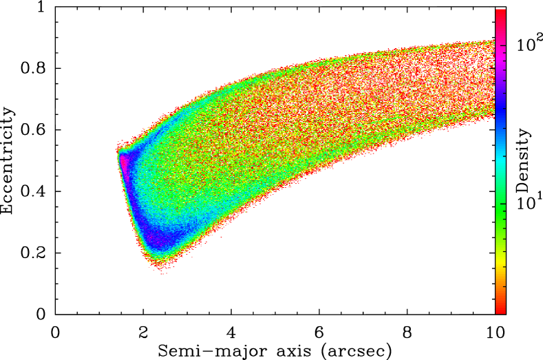
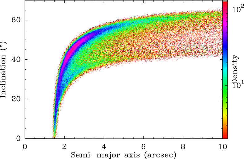
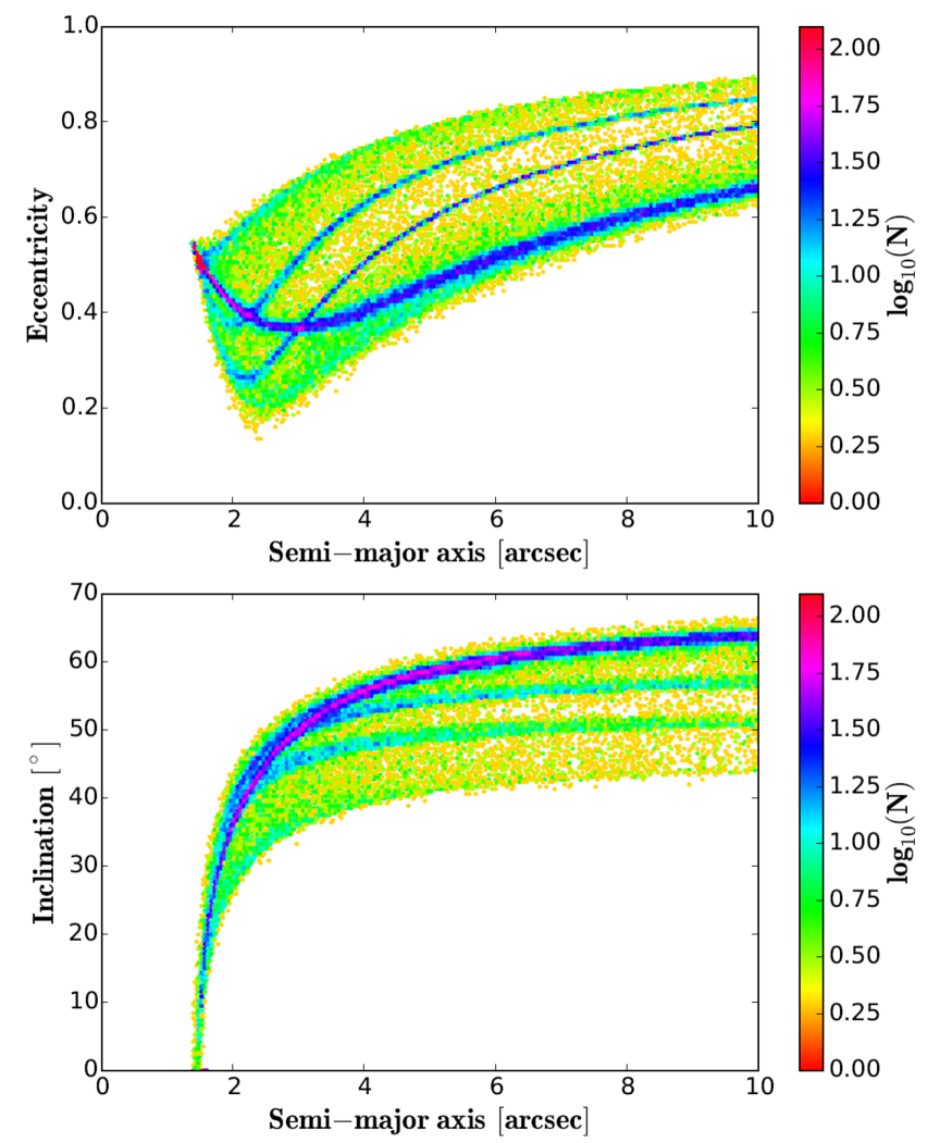
Figure 14: Left and Middle: Additional plots to Fig. 13 restricted to bound orbits only recovered by our MCMC fit, showing i/ posterior distributions of semi-major axis and orbital period (left), ii/ bidimensional density maps involving the semi-major axis $a$ versus the eccentricity $e$ and the inclination $i$. The color scale appearing on the right side of the plots also applies to all similar plots of Fig. 13. Right: The same bidimensional density maps as shown in Fig. 14 showing orbit solutions recovered by our LSMC fit with semi-major axes smaller than 10″.

To better compare LSMC and MCMC results we created matching bidimensional density maps restricted to bound orbits, considering the semi-major axis $a$ and the eccentricity $e$ as well as the inclination $i$. For the MCMC results we restricted ourselfs to bound solutions only. To match the MCMC results closely we cut off the LSMC results at semi-major axes smaller than 10″. The results are shown in Fig. 14. We first show posterior MCMC distribution for the semi-major axis and the orbital period (left plots). We see that although both histograms exhibit tails towards large values (and thus approaching unbound orbits), clear peaks appears around $\sim 40\,$AU and $\sim 200\,$yr. Those values must be regarded as the most probable ones. Then we come to comparing the 2D maps generated by MCMC and LSMC (middle and right plots). This immediate comparison shows that both approaches agree very well to derive the same well-fitting range of bound orbital solutions. The differences in the density of solutions are likely caused by the difference of prior distributions used as input for both methods. While for LSMC uniform distributions in $a$ and $i$ were considered we used distributions that were uniform in $log\,q$ and $\propto\sin i$ for $i$. This was done because the aim of the methods is somewhat different. With LSMC we aim to find the full possible range of geometrically well fitting orbits, as well as the best fitting orbit in terms of $\chi^{2}_{red}$. With MCMC, on the other hand, the goal is to find the correct posterior probability distribution given our prior knowledge of the system. This knowledge includes that shorter period orbits are more likely given were we find the companion in our observation epochs as well as the statistical likelyhood of orbit inclinations.

We want to stress that the general results obtained by both methods agree very well. In particular with LSMC we find an upper limit of the inclination of bound orbits of 70.8 deg, while the upper limit of the 1 $\sigma$ confidence interval recovered by LSMC is 70.3 deg. Both methods also find strong peaks in the time of the periastron passage between the years 2039 and 2040. The MCMC fit furthermore recovered 68 % of bound orbit solutions. Given this high likelyhood of a bound orbit and the large chance for a periastron passage within the next few decades, the GJ 758 system remains an interesting target for continued orbital monitoring. It is likely that orbit curvature will be discovered in this timeframe, allowing for a much better constrained determination of the companions orbit.

7 Sensitivity to additional companions

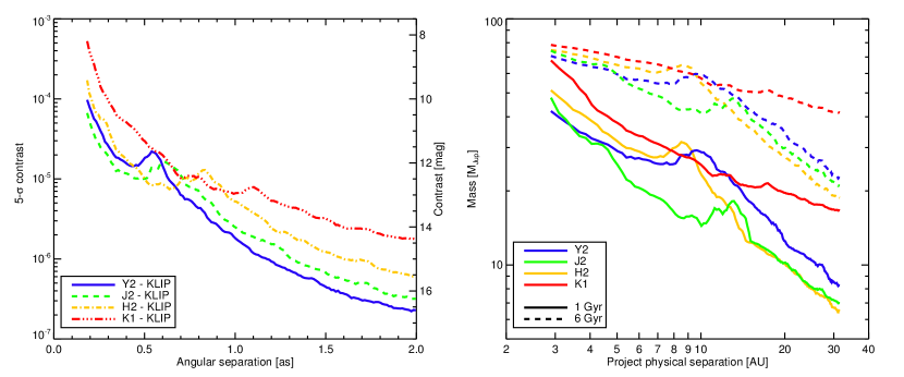
Figure 15: Left: 5-$\sigma$ detection limits measured in the Y2, J2, H2 and K1 filters using a KLIP analysis, with a number of subtracted modes that varies to maximize the algorithm throughput. Right: Conversion of these detection limits into physical units using the known distance of the GJ 758 system (15.76 pc) and the AMES-COND evolutinary tracks (Baraffe et al. 2003) calculated in the IRDIS filters. Two sets of curves assuming the two extremes of the system age range (1 and 6 Gyr, see Sect. 4) are displayed. The limits for the nominal age of 3 Gyr lie in-between, slightly closer to the the 6 Gyr limit than the 1 Gyr limit.

To conclude our analysis, it is interesting to look at our sensitivity to additional massive companions in the GJ 758 system. We calculated detection limits in the different DBI filters following an ADI analysis with KLIP. The limits were estimated by measuring the standard deviation of the residuals in annuli of width 1 $\lambda/D$ at increasing angular separation, divided by the maximum of the off-axis PSF of the star in the same filter. To properly take into account the effect of self-subtraction induced on the detection limits, the algorithm throughput was estimated by injecting fake companions regularly spaced from 0.1″to 2.0″into the pre-processed data cubes. They were injected at a level 10 times higher than the noise residuals in the final images at the separation of each of the companions. This process was repeated 10 times with different orientations of the pattern of fake companions to average out possible variations of the throughput as a function of the position in the field. The throughput at each separation was then calculated to be the mean throughput over the 10 measurements.

The final detection limits taking into account the throughput in the different filters are plotted in the right panel of Fig. 15. Due to the small amount of field rotation in all observing sequences ($\lesssim$8^o), the throughput of the analysis decreases significantly towards small angular separations, resulting in a sharp deterioration of the detection limits. It is only at separations larger than 0.21″, 0.25″, 0.33″and 0.43″that the field rotates by more than $\lambda/D$ over the course of the complete sequence in $Y$-, $J$-, $H$- and $K$-band respectively. The sensitivity is nonetheless improved compared previous measurement below $\sim$0.5″, in particular for this specific target.

The right panel of Fig. 15 shows the conversion of these detection limits into physical units of projected separation and physical mass, using the known distance of the star (15.76 pc) and the AMES-COND evolutionary models (Baraffe et al. 2003) calculated in the IRDIS DBI filters. The two sets of curves represent the limit for the two extremes of the system’s age range, 1–6 Gyr (see Sect. 4). For the youngest part of the age range, our observations clearly probe the low mass brown-dwarf regime down to 4–5 AU, and even the planetary-mass regime beyond 20–30 AU. However, if we assume an older age for the system, more in line with the different age indicators, only massive brown-dwarfs could be detected.

8 Summary & conclusions

Our new study of GJ 758 offers an improved overview of this interesting system. The brown-dwarf companion is redetected and we confirm some of its already known properties using our finer spectral sampling from SPHERE/IRDIS observations. In particular, we recover a low $T_{e\!f\!f}=600\pm 100$ K from comparison to 4 different sets of models, in good agreement with previous studies (Thalmann et al. 2009; Currie et al. 2010; Janson et al. 2011). There are however some interesting peculiarities that are worth discussing.

From comparison to empirical objects, GJ 758 B appears as a very interesting object because we cannot find objects with known age and metallicity that matches all of its observed fluxes. We estimate a T8 spectral type for this object, but this estimation is limited by the small amount of spectra of T8–T9 dwarfs with robust constraints on their age and metallicity. One of the most likely explanations for the peculiar SED of this brown dwarf is the super-solar metallicity of the primary (${\rm[Fe/H]}=0.18\pm 0.05$; see Sect. 4.2), and of the companion if we assume they share the same metal enrichment. This is supported by the fact that the T8pec companion to the metal-poor dwarf BD+01 292 (Pinfield et al. 2012) shows a $K$-band spectral deviation opposite to that of GJ 758 B. Unfortunately, the current lack of such companions precludes us to perform a meaningful comparison. Similarly, comparison to synthetic grids of models are constrained by the limited extension of most grids toward non-solar metallicities and low $T_{e\!f\!f}$ values. None of the four types of models that we tested were able to reproduce accurately the photometry of GJ 758 B in all filters. Especially, the J3 and H2 fluxes are very hard to reproduce and cannot be readily explained with any of the models. The BT-SETTL14 models (Allard et al. 2013), with an enrichment of 0.3 dex in $\alpha$ elements with respect to solar, do provide a better fit of the J3 flux, but at the price of much smaller dilution factors corresponding to unphysical values of the companion radius ($\sim$0.7 $R_{\mathrm{Jup}}$). Even so, the high H2 flux is not reproduced. This could actually indicate that the $T_{e\!f\!f}$ of GJ 758 B might be even lower than the one of the best fit, but we are limited by the absence of metal-enriched models at very low $T_{e\!f\!f}$. As a result, our analysis confirms the low $T_{e\!f\!f}$ of the object, corresponding to a mass of $23^{+17}_{-13}$ $M_{\mathrm{Jup}}$ in the considered age range (using the Baraffe et al. 2003 evolutionary tracks), but we cannot infer any precise value for $\log\leavevmode\nobreak\ g$ and M/H. The study of this object would strongly benefit from low-resolution spectroscopy, e.g. with IRDIS long-slit spectroscopy mode (Vigan et al. 2008).

The new astrometry confirms the picture of a very eccentric companion. Similarly to what was reported by Janson et al. (2011), the curvature of the orbit is still not detectable yet. The $\sim$0.28″motion of the companion along its orbit appears roughly as a straight line from the previous measurements from 2010. Our LSMC and MCMC simulations favour an eccentric – but bound – orbit, with high-likelihood of $e\simeq 0.5$. In particular, no orbital solution shows an eccentricity lower than 0.14, which is consistent with previously reported results and between our two approaches ([0.133–1.78] 95% confidence interval from MCMC). In addition, we have ruled out the possibility that the observed eccentricity is just caused by a massive closer-in companion that would create a false positive eccentricity by astrometric displacement of the primary. Indeed, although not extremely accurate, our RV data reject companion more massive then 0.02 $M_{\odot}$ on periods shorter than 17 years and inclination larger than 5 deg. Finally, our new IRDIS observations reject the possibility of an additional companion more massive than $\sim$30-40 $M_{\mathrm{Jup}}$ (for ages of 1-3 Gyr) above 4-5 AU.

In light of our constraints on the orbit and mass of GJ 758 B, it is interesting to look into the formation of this object. While our study does not bring enough new material in favor or against planet-like formation scenarios (core accretion vs. gravitational instability, migration, etc), we can instead focus on stellar-like formation scenarios. Several past studies have argued for a universal companion mass function (CMF) for stellar and sub-stellar companions. In particular, in their in-depth anaysis focused on brown dwarfs around solar-type stars, Metchev & Hillenbrand (2009) find tentative evidence for such a universal CMF and predict a peak in semi-major axes for brown dwarfs at $\sim$30 AU. From that point of view, it makes sense to compare the properties of the GJ 758 system to the properties of solar-type multiple systems. (Raghavan et al. 2010) have published the most complete study on this topic to date. While we cannot compare quantitatively our results on a single object with their global multiplicity analysis, it is interesting to note a few qualitative facts. Firstly, with a most likely period of 312.48 yr (from MCMC, see Table 10), GJ 758 B falls exactly at the peak of their period distribution (293.57 yr; their Fig. 13). Secondly, with a most likely eccentricity of 0.525, GJ 758 B falls in the bulk of their eccentricity–period distributions. And thirdly, with a ratio $q=M_{2}/M_{1}=0.023\pm 0.013$, the GJ 758 systems falls at the very edge of the study of (Raghavan et al. 2010), but in their $q$–period plot, the system is not completely isolated and could be part of the tail of the distribution. While these facts do not prove that the system was formed in a stellar way, they certainly support the possibility qualitatively.

In conclusion, GJ 758 B remains a very interesting object that warrants deeper observations to look for additional companions in the system, spectroscopic observations to better constrain its physical properties, and astrometric monitoring to get tighter constraints on its eccentric orbit.

Appendix A Description of the atmospheric models

The specificity of the models in the range of $T_{e\!f\!f}$ suited for GJ 758 B are not all described in the literature yet. So it is important to make a description of the most relevant hypothesis in the models and differences between the models in this paper. The parameter space of the models is summarised in Table 11.

The BT-Settl model couples a cloud model to a 1D radiative transfer code PHOENIX (Allard et al. 1994; Hauschildt et al. 1997). The model considers the formation of a cloud deck composed of up to 55 grain species. The grain size and density, the abundances of chemicals in the gas phase, including the effect of element depletion induced by the grain formation, is computed layer per layer through the photosphere following a comparison of the timescales for nucleation, condensation, gravitational settling or sedimentation, and mixing. Once rained out below the photosphere, the grain opacities are not accounted for into the radiative transfer. Nevertheless, these grains can still interact chemically with the gas phase. These models can predict the flux at the surface of a given object only defined by $\log\leavevmode\nobreak\ g$, $T_{e\!f\!f}$, and [Fe/H]. They account for the non-equilibrium chemistry of CO, CH₄, N₂, NH₃, and CO₂. The models predict the formation of a secondary (resurgent) cloud layer into the photosphere made of Na₂S and MnS then of KCl, NaCl and some ZnS that lies above the rained-out primary cloud layer located below the photosphere and that originally sustains in the atmosphere of L and early-T dwarfs. Here we used the 2014 releases of the models (hereafter BT-SETTL14) which include revised alkali cloud opacities and the latest CIA opacities (Abel et al. 2012). A specific grid was computed for the project to cover the Y-dwarf temperature domain (hereafter BT-SETTL14-Y) in addition to the already existing grid covering a broader interval of $T_{e\!f\!f}$ and considering $\alpha$-element enrichment (hereafter BT-SETTL14).

The 1D Exo-REM models (Baudino, J.L. et al. 2015) propose a simplified approach of sub-stellar atmospheres. They predict the equilibrium-temperature profile and mixing-ratio profiles of the most important gases (H2-He collision-induced absorption, H₂O, CO, CH₄, NH₃, VO, TiO, Na, and K). The absorption by iron and silicate cloud particles is added above the expected condensation levels with a fixed scale height and a given optical depth at some reference wavelength. For the purpose of the GJ 758 B study, two grids of models – NC and T3 – were computed. The NC models consider photospheres with no cloud opacity. The T3 models consider a photosphere with 30 $\mu$m Iron (Fe) and Forsterite (Mg₂SiO₄) grains and an optical depth of reference $\mathrm{\tau_{cloud}}=3$. The grains are located between condensation level and a 100 times lower pressure. They have scale heights equal to the gas scale height, and optical depths of 3 and 0.45 at 1.2 $\mu$m respectively for Fe and Mg₂SiO₄.

Similarly to the BT-Settl models, the Morley+12 models account for the possible resurgence of clouds in late-T dwarf atmospheres. These 1D models build on the cloud model of Ackerman & Marley (2001). The cloud content (and opacity) is determined by a balance between the upward transport by turbulent mixing with the sedimentation. The Ackerman & Marley (2001) models do not compute the microphysics associated to the clouds, and rather let as free parameters the vertical eddy diffusion coefficient $K_{zz}$ and a sedimentation efficiency parameter $f_{sed}$. A higher $f_{sed}$ correspond to thinner (rained-out) clouds. For the case of the Morley+12 models, non-equilibrium chemistry is not included, so only models with $K_{zz}=0$ are available. The models only enable an exploration of the $f_{sed}$. As a second difference with the BT-Settl, the Morley+12 models do not account for chemical reactions between the condensed species and the gas phase. Finally, we added to this grid the models of Saumon et al. (2012), also based on Ackerman & Marley (2001) models, to explore the case of an extreme sedimentation efficiency (cloud-free atmospheres).

Table 11: Characteristics of the atmospheric model grids adjusted on the SED of GJ 758 B. [$\alpha$] stands for the $\alpha$ elements enhancement with respect to solar (Caffau et al. 2011).

Model name	$T_{e\!f\!f}$	$\Delta T_{e\!f\!f}$	$\log\leavevmode\nobreak\ g$	$\Delta\log\leavevmode\nobreak\ g$	[M/H]	$[\alpha]$	$f_{SED}$
	(K)	(K)	(dex)	(dex)	(dex)	(dex)
BT-SETTL14-Y	200-420	20	3.5-4.5	0.5	0.0	0.0	n/a
BT-SETTL14-Y	450-1000	50	3.5-4.5	0.5	0.0	0.0	n/a
BT-SETTL14	500-3000	50	3.5-5.5	0.5	0.0	0.0	n/a
BT-SETTL14	500-2800	100	4.0-5.5	0.5	0.0	0.3	n/a
Exo-REM - NC	400-1300	100	3.5-5.5	0.2	-0.5,0,+0.5	0.0	n/a
Exo-REM - T3	400-1300	100	3.5-5.5	0.2	-0.5,0,+0.5	0.0	n/a
Morley+12	400-600	50	4.0-5.5	0.5	0.0	0.0	2,3,4,5
Morley+12	600-1200	100	4.0-5.5	0.5	0.0	0.0	2,3,4,5
Saumon+12	300-350	50	3.75,4.0-5.0	0.25,0.5	0.0	0.0	$\infty$
Saumon+12	300-1200	50	3.0-4.75,5.0-5.5	0.25,0.5	0.0	0.0	$\infty$
Saumon+12	1300-1500	100	4.0-5.0	0.5	0.0	0.0	$\infty$

References

- Abel et al. (2012) Abel, M., Frommhold, L., Li, X., & Hunt, K. L. C. 2012, in APS Meeting Abstracts, 26001
- Ackerman & Marley (2001) Ackerman, A. S. & Marley, M. S. 2001, ApJ, 556, 872
- Allard et al. (1994) Allard, F., Hauschildt, P. H., Miller, S., & Tennyson, J. 1994, ApJ, 426, L39
- Allard et al. (2013) Allard, F., Homeier, D., Freytag, B., et al. 2013, Memorie della Societa Astronomica Italiana Supplementi, 24, 128
- Baraffe et al. (2003) Baraffe, I., Chabrier, G., Barman, T. S., Allard, F., & Hauschildt, P. H. 2003, A&A, 402, 701
- Baranne et al. (1979) Baranne, A., Mayor, M., & Poncet, J. L. 1979, Vistas in Astronomy, 23, 279
- Baudino, J.L. et al. (2015) Baudino, J.L., Bézard, B., Boccaletti, A., et al. 2015, A&A
- Bellini et al. (2014) Bellini, A., Anderson, J., van der Marel, R. P., et al. 2014, ApJ, 797, 115
- Beust et al. (2014) Beust, H., Augereau, J.-C., Bonsor, A., et al. 2014, A&A, 561, A43
- Beuzit et al. (2008) Beuzit, J.-L., Feldt, M., Dohlen, K., et al. 2008, in SPIE Conference Series, Vol. 7014, 18
- Boccaletti et al. (2008) Boccaletti, A., Abe, L., Baudrand, J., et al. 2008, in SPIE Conference Series, Vol. 7015, 1
- Bohlin (2007) Bohlin, R. C. 2007, in Astronomical Society of the Pacific Conference Series, Vol. 364, The Future of Photometric, Spectrophotometric and Polarimetric Standardization, ed. C. Sterken, 315
- Borysow et al. (1997) Borysow, A., Jorgensen, U. G., & Zheng, C. 1997, A&A, 324, 185
- Bowler et al. (2010) Bowler, B. P., Liu, M. C., Dupuy, T. J., & Cushing, M. C. 2010, ApJ, 723, 850
- Bressan et al. (2012) Bressan, A., Marigo, P., Girardi, L., et al. 2012, MNRAS, 427, 127
- Brott & Hauschildt (2005) Brott, I. & Hauschildt, P. H. 2005, in ESA Special Publication, Vol. 576, The Three-Dimensional Universe with Gaia, ed. C. Turon, K. S. O’Flaherty, & M. A. C. Perryman, 565
- Buenzli et al. (2012) Buenzli, E., Apai, D., Morley, C. V., et al. 2012, ApJ, 760, L31
- Burgasser (2014) Burgasser, A. J. 2014, in Astronomical Society of India Conference Series, Vol. 11, Astronomical Society of India Conference Series, 7–16
- Burgasser et al. (2011) Burgasser, A. J., Cushing, M. C., Kirkpatrick, J. D., et al. 2011, ApJ, 735, 116
- Burgasser et al. (2004) Burgasser, A. J., McElwain, M. W., Kirkpatrick, J. D., et al. 2004, AJ, 127, 2856
- Burgasser et al. (2010) Burgasser, A. J., Simcoe, R. A., Bochanski, J. J., et al. 2010, ApJ, 725, 1405
- Burkardt & Danby (1983) Burkardt, T. M. & Danby, J. M. A. 1983, Celestial Mechanics, 31, 317
- Burningham et al. (2011) Burningham, B., Leggett, S. K., Homeier, D., et al. 2011, MNRAS, 414, 3590
- Burningham et al. (2009) Burningham, B., Pinfield, D. J., Leggett, S. K., et al. 2009, MNRAS, 395, 1237
- Burrows et al. (2006) Burrows, A., Sudarsky, D., & Hubeny, I. 2006, ApJ, 640, 1063
- Caffau et al. (2011) Caffau, E., Ludwig, H.-G., Steffen, M., Freytag, B., & Bonifacio, P. 2011, Sol. Phys., 268, 255
- Chauvin et al. (2012) Chauvin, G., Lagrange, A.-M., Beust, H., et al. 2012, A&A, 542, A41
- Chauvin et al. (2015) Chauvin, G., Vigan, A., Bonnefoy, M., et al. 2015, A&A, 573, A127
- Close et al. (2003) Close, L. M., Siegler, N., Freed, M., & Biller, B. 2003, ApJ, 587, 407
- Currie et al. (2010) Currie, T., Bailey, V., Fabrycky, D., et al. 2010, ApJ, 721, L177
- Cushing et al. (2008) Cushing, M. C., Marley, M. S., Saumon, D., et al. 2008, ApJ, 678, 1372
- Cushing et al. (2005) Cushing, M. C., Rayner, J. T., & Vacca, W. D. 2005, ApJ, 623, 1115
- Cutri & et al. (2013) Cutri, R. M. & et al. 2013, VizieR Online Data Catalog, 2328, 0
- Cutri et al. (2003) Cutri, R. M., Skrutskie, M. F., van Dyk, S., et al. 2003, 2MASS All Sky Catalog of point sources.
- da Silva et al. (2006) da Silva, L., Girardi, L., Pasquini, L., et al. 2006, A&A, 458, 609
- Danby (1987) Danby, J. M. A. 1987, Celestial Mechanics, 40, 303
- Danby & Burkardt (1983) Danby, J. M. A. & Burkardt, T. M. 1983, Celestial Mechanics, 31, 95
- De Silva et al. (2013) De Silva, G. M., D’Orazi, V., Melo, C., et al. 2013, MNRAS, 431, 1005
- Desidera et al. (2015) Desidera, S., Covino, E., Messina, S., et al. 2015, A&A, 573, A126
- Desidera et al. (2011) Desidera, S., Covino, E., Messina, S., et al. 2011, A&A, 529, A54
- Dohlen et al. (2008) Dohlen, K., Langlois, M., Saisse, M., et al. 2008, in SPIE Conference Series, Vol. 7014, 3
- D’Orazi et al. (2012) D’Orazi, V., Biazzo, K., Desidera, S., et al. 2012, MNRAS, 423, 2789
- D’Orazi et al. (2009a) D’Orazi, V., Magrini, L., Randich, S., et al. 2009a, ApJ, 693, L31
- D’Orazi et al. (2009b) D’Orazi, V., Magrini, L., Randich, S., et al. 2009b, ApJ, 693, L31
- D’Orazi & Randich (2009) D’Orazi, V. & Randich, S. 2009, A&A, 501, 553
- Duncan et al. (1991) Duncan, D. K., Vaughan, A. H., Wilson, O. C., et al. 1991, ApJS, 76, 383
- Dupuy & Kraus (2013) Dupuy, T. J. & Kraus, A. L. 2013, Science, 341, 1492
- Faherty et al. (2012) Faherty, J. K., Burgasser, A. J., Walter, F. M., et al. 2012, ApJ, 752, 56
- Fischer et al. (2014) Fischer, D. A., Marcy, G. W., & Spronck, J. F. P. 2014, ApJS, 210, 5
- Ford (2006) Ford, E. B. 2006, ApJ, 642, 505
- Fusco et al. (2006) Fusco, T., Rousset, G., Sauvage, J.-F., et al. 2006, Optics Express, 14, 7515
- Fusco et al. (2014) Fusco, T., Sauvage, J.-F., Petit, C., et al. 2014, in SPIE Conference Series, Vol. 9148, 15
- Gagné et al. (2014) Gagné, J., Lafrenière, D., Doyon, R., Malo, L., & Artigau, É. 2014, ApJ, 783, 121
- Galicher & Marois (2011) Galicher, R. & Marois, C. 2011, in Second International Conference on Adaptive Optics for Extremely Large Telescopes. Online at ¡A href=”http://ao4elt2.lesia.obspm.fr”¿http://ao4elt2.lesia.obspm.fr¡/A¿, id.P25, 25P
- Geballe et al. (1996) Geballe, T. R., Kulkarni, S. R., Woodward, C. E., & Sloan, G. C. 1996, ApJ, 467, L101
- Geballe et al. (2001) Geballe, T. R., Saumon, D., Leggett, S. K., et al. 2001, ApJ, 556, 373
- Ginski et al. (2013) Ginski, C., Neuhäuser, R., Mugrauer, M., Schmidt, T. O. B., & Adam, C. 2013, MNRAS, 434, 671
- Goldman et al. (2010) Goldman, B., Marsat, S., Henning, T., Clemens, C., & Greiner, J. 2010, MNRAS, 405, 1140
- Hauschildt et al. (1997) Hauschildt, P. H., Baron, E., & Allard, F. 1997, ApJ, 483, 390
- Hoeg et al. (1997) Hoeg, E., Bässgen, G., Bastian, U., et al. 1997, A&A, 323, L57
- Hugot et al. (2012) Hugot, E., Ferrari, M., El Hadi, K., et al. 2012, A&A, 538, A139
- Isaacson & Fischer (2010) Isaacson, H. & Fischer, D. 2010, ApJ, 725, 875
- Jacobson & Friel (2013) Jacobson, H. R. & Friel, E. D. 2013, AJ, 145, 107
- Janson et al. (2011) Janson, M., Carson, J., Thalmann, C., et al. 2011, ApJ, 728, 85
- Jarrett et al. (2011) Jarrett, T. H., Cohen, M., Masci, F., et al. 2011, ApJ, 735, 112
- Jones et al. (2013) Jones, A., Noll, S., Kausch, W., Szyszka, C., & Kimeswenger, S. 2013, A&A, 560, A91
- Kalas et al. (2013) Kalas, P., Graham, J. R., Fitzgerald, M. P., & Clampin, M. 2013, ApJ, 775, 56
- Kovtyukh et al. (2004) Kovtyukh, V. V., Soubiran, C., & Belik, S. I. 2004, A&A, 427, 933
- Kurucz (1993) Kurucz, R. 1993, ATLAS9 Stellar Atmosphere Programs and 2 km/s grid. Kurucz CD-ROM No. 13. Cambridge, Mass.: Smithsonian Astrophysical Observatory, 1993., 13
- Leggett et al. (2001) Leggett, S. K., Allard, F., Geballe, T. R., Hauschildt, P. H., & Schweitzer, A. 2001, ApJ, 548, 908
- Leggett et al. (2010) Leggett, S. K., Burningham, B., Saumon, D., et al. 2010, ApJ, 710, 1627
- Lucas et al. (2010) Lucas, P. W., Tinney, C. G., Burningham, B., et al. 2010, MNRAS, 408, L56
- Mace et al. (2013) Mace, G. N., Kirkpatrick, J. D., Cushing, M. C., et al. 2013, ApJ, 777, 36
- Macintosh et al. (2014) Macintosh, B., Graham, J. R., Ingraham, P., et al. 2014, Proceedings of the National Academy of Science, 111, 12661
- Maiorca et al. (2012) Maiorca, E., Magrini, L., Busso, M., et al. 2012, ApJ, 747, 53
- Maire et al. (2014) Maire, A.-L., Boccaletti, A., Rameau, J., et al. 2014, A&A, 566, A126
- Maldonado et al. (2012) Maldonado, J., Eiroa, C., Villaver, E., Montesinos, B., & Mora, A. 2012, A&A, 541, A40
- Malo et al. (2013) Malo, L., Doyon, R., Lafrenière, D., et al. 2013, ApJ, 762, 88
- Mamajek & Hillenbrand (2008) Mamajek, E. E. & Hillenbrand, L. A. 2008, ApJ, 687, 1264
- Markwardt (2009) Markwardt, C. B. 2009, in Astronomical Society of the Pacific Conference Series, Vol. 411, Astronomical Data Analysis Software and Systems XVIII, ed. D. A. Bohlender, D. Durand, & P. Dowler, 251
- Marois et al. (2014) Marois, C., Correia, C., Véran, J.-P., & Currie, T. 2014, in IAU Symposium, Vol. 299, IAU Symposium, ed. M. Booth, B. C. Matthews, & J. R. Graham, 48–49
- Marois et al. (2006) Marois, C., Lafrenière, D., Doyon, R., Macintosh, B., & Nadeau, D. 2006, ApJ, 641, 556
- Marois et al. (2010) Marois, C., Macintosh, B., & Véran, J.-P. 2010, in SPIE Conference Series, Vol. 7736
- McLean et al. (2003) McLean, I. S., McGovern, M. R., Burgasser, A. J., et al. 2003, ApJ, 596, 561
- Metchev & Hillenbrand (2009) Metchev, S. A. & Hillenbrand, L. A. 2009, ApJS, 181, 62
- Mishenina et al. (2013) Mishenina, T., Korotin, S., Carraro, G., Kovtyukh, V. V., & Yegorova, I. A. 2013, MNRAS, 433, 1436
- Monet et al. (2003) Monet, D. G., Levine, S. E., Canzian, B., et al. 2003, AJ, 125, 984
- Morley et al. (2012) Morley, C. V., Fortney, J. J., Marley, M. S., et al. 2012, ApJ, 756, 172
- Moultaka et al. (2004) Moultaka, J., Ilovaisky, S. A., Prugniel, P., & Soubiran, C. 2004, PASP, 116, 693
- Neves et al. (2014) Neves, V., Bonfils, X., Santos, N. C., et al. 2014, A&A, 568, A121
- Nidever et al. (2002) Nidever, D. L., Marcy, G. W., Butler, R. P., Fischer, D. A., & Vogt, S. S. 2002, ApJS, 141, 503
- Nielsen et al. (2014) Nielsen, E. L., Liu, M. C., Wahhaj, Z., et al. 2014, ApJ, 794, 158
- Noll et al. (2012) Noll, S., Kausch, W., Barden, M., et al. 2012, A&A, 543, A92
- Pavlov et al. (2008) Pavlov, A., Möller-Nilsson, O., Feldt, M., et al. 2008, in SPIE Conference Series, Vol. 7019, 39
- Pearce et al. (2014) Pearce, T. D., Wyatt, M. C., & Kennedy, G. M. 2014, MNRAS, 437, 2686
- Pearce et al. (2015) Pearce, T. D., Wyatt, M. C., & Kennedy, G. M. 2015, ArXiv e-prints
- Petit et al. (2014) Petit, C., Sauvage, J.-F., Fusco, T., et al. 2014, in SPIE Conference Series, Vol. 9148, 0
- Pinfield et al. (2012) Pinfield, D. J., Burningham, B., Lodieu, N., et al. 2012, MNRAS, 422, 1922
- Pueyo et al. (2014) Pueyo, L., Soummer, R., Hoffmann, J., et al. 2014, ArXiv e-prints
- Racine et al. (1999) Racine, R., Walker, G. A. H., Nadeau, D., Doyon, R., & Marois, C. 1999, PASP, 111, 587
- Raghavan et al. (2010) Raghavan, D., McAlister, H. A., Henry, T. J., et al. 2010, ApJS, 190, 1
- Rayner et al. (2009) Rayner, J. T., Cushing, M. C., & Vacca, W. D. 2009, ApJS, 185, 289
- Saumon et al. (1994) Saumon, D., Bergeron, P., Lunine, J. I., Hubbard, W. B., & Burrows, A. 1994, ApJ, 424, 333
- Saumon & Marley (2008) Saumon, D. & Marley, M. S. 2008, ApJ, 689, 1327
- Saumon et al. (2012) Saumon, D., Marley, M. S., Abel, M., Frommhold, L., & Freedman, R. S. 2012, ApJ, 750, 74
- Sauvage et al. (2014) Sauvage, J.-F., Fusco, T., Petit, C., et al. 2014, in SPIE Conference Series, Vol. 9148
- Scholz (2010) Scholz, R.-D. 2010, A&A, 515, A92
- Sneden (1973) Sneden, C. A. 1973, PhD thesis, THE UNIVERSITY OF TEXAS AT AUSTIN.
- Soubiran et al. (2008) Soubiran, C., Bienaymé, O., Mishenina, T. V., & Kovtyukh, V. V. 2008, A&A, 480, 91
- Soummer (2005) Soummer, R. 2005, ApJ, 618, L161
- Soummer et al. (2012) Soummer, R., Pueyo, L., & Larkin, J. 2012, ApJ, 755, L28
- Takeda et al. (2007) Takeda, G., Ford, E. B., Sills, A., et al. 2007, ApJS, 168, 297
- Takeda (2007) Takeda, Y. 2007, PASJ, 59, 335
- Takeda & Kawanomoto (2005) Takeda, Y. & Kawanomoto, S. 2005, PASJ, 57, 45
- Thalmann et al. (2009) Thalmann, C., Carson, J., Janson, M., et al. 2009, ApJ, 707, L123
- van Leeuwen (2007) van Leeuwen, F. 2007, A&A, 474, 653
- Vigan et al. (2008) Vigan, A., Langlois, M., Moutou, C., & Dohlen, K. 2008, A&A, 489, 1345
- Vigan et al. (2010) Vigan, A., Moutou, C., Langlois, M., et al. 2010, MNRAS, 407, 71
- Vigan et al. (2012) Vigan, A., Patience, J., Marois, C., et al. 2012, A&A, 544, A9
- Voges et al. (1999) Voges, W., Aschenbach, B., Boller, T., et al. 1999, A&A, 349, 389
- Voges et al. (2000) Voges, W., Aschenbach, B., Boller, T., et al. 2000, IAU Circ., 7432, 1
- Wright et al. (2004) Wright, J. T., Marcy, G. W., Butler, R. P., & Vogt, S. S. 2004, ApJS, 152, 261
- Yong et al. (2012) Yong, D., Carney, B. W., & Friel, E. D. 2012, AJ, 144, 95