Adsorption of highly charged Gaussian polyelectrolytes to oppositely charged surfaces

Abstract

In many biological processes highly charged biomolecules are adsorbed into oppositely charged surfaces of macroions and membranes. They form strongly correlated structures close to the surface which can not be explained by the conventional Poisson-Boltzmann theory. Many of the flexible biomolecules can be described by Gaussian polymers. In this work strong coupling theory is used to study the adsorption of highly charged Gaussian polyelectrolytes. Two cases of adsorptions are considered, when the Gaussian polyelectrolytes are confined a) by one charged wall, and b) between two charged walls. The effects of salt and the geometry of the polymers on their adsorption-depletion transitions in the strong coupling regime are discussed.

I Introduction

The phenomenon of polymer adsorption is of great interest in biological sciences as it is the key mechanism behind many of the biological processes like DNA winding around nucleosome cores Luger et al. (1997); Cherstvy (2009), binding of genomes in RNA viruses by capsid proteins Belyi and Muthukumar (2006); Forrey and Muthukumar (2009), tau association to microtubules Jho et al. (2010) and polyelectrolyte multilayer vesicles Caruso et al. (1999). Of particular interest is that of adsorption caused by electrostatic forces as many biomolecules like DNA and RNA are highly charged and they frequently bind themselves to oppositely charged protein or membrane surfaces. There is an extensive literature both in theory Baumgärtner and Muthukumar (1991); Von Goeler and Muthukumar (1994); Linse (1996); Shafir et al. (2003); Winkler and Cherstvy (2006); Man et al. (2008); Ličer and Podgornik (2010); Wang et al. (2011); Cherstvy and Winkler (2012); De Gennes (1979); Podgornik (1990) as well as in simulations Chodanowski and Stoll (2001); Kong and Muthukumar (1998); Welch and Muthukumar (2000); Messina et al. (2004); Ulrich et al. (2005); Forsman (2012); Xie et al. (2013); Stoll and Chodanowski (2002); Källrot and Linse (2010); Ulrich et al. (2006); Cao et al. (2011); Carnal and Stoll (2011); Cerdà et al. (2009); Jeong et al. (2014) on electrostatic driven adsorption of flexible polyelectrolyte (PE) chains onto surfaces. Experimental studies have also been performed to investigate the dependence of the critical adsorption threshold on the PE charges, salt concentration and the surface charge density of the fixed charge distribution McQuigg et al. (1992); Feng et al. (2001); Kayitmazer et al. (2005); Cherstvy and Winkler (2011). A PE is adsorbed into a surface when the electrostatic attractions between the PE and the surface overcomes the entropy of the PE chain. The presence of salt plays an important role in the adsorption process as higher salt concentration screens the electrostatic attractions thus inhibiting adsorption.

Several theoretical models exist to describe PE adsorption into charged surfaces. Most of these models use mean field description Châtellier and Joanny (1996); Joanny (1999); Wiegel (1977); Muthukumar (1987), various scaling theories Borukhov et al. (1998, 1995); Borisov et al. (1994); Dobrynin et al. (2001, 2000); Dobrynin and Rubinstein (2005) or other phenomenological criteria for adsorption Netz and Joanny (1999); Netz and Andelman (2003). Wiegel Wiegel (1977) was one of the first to obtain a closed expression for the adsorption threshold for Gaussian polyelectrolytes (GPEs) in the mean field approximation using polymer field theory. Muthukumar Muthukumar (1987) later extended this work to include excluded volume interactions among PE chains. In references Shafir et al. (2003); Borukhov et al. (1998, 1995) a coupled Poisson – Boltzmann and Edwards polymer density equations Edwards (1965) have been used to obtain scaling laws for adsorption-depletion transitions for PEs. Dobrynin et al. Dobrynin et al. (2000, 2001) proposed a Wigner liquid structure for the adsorbed polyelectrolyte layer based on the idea of counterion condensation by Shklovskii Shklovskii (1999a, b); Perel and Shklovskii (1999); Grosberg et al. (2002). The conventional Poisson-Boltzmann formalism fails inside the Wigner layer and strong coupling (SC) theories Netz (2001); Moreira and Netz (2001); Shklovskii (1999a); Kanduč et al. (2009); Naji et al. (2013); Levin (2002); Naji (2005); Boroudjerdi et al. (2005); Grosberg et al. (2002) are more appropriate descriptions in these domains. In fact many highly charged biomolecules act as multivalent counterions with strong many-body correlations and the strong coupling theories, which were developed to explain the like-charged attractions in multivalent counterions (for which the Coulomb coupling is large $\Xi>>1$ as opposed to the mean field approximation which is valid in the weak coupling $\Xi<1$), provide a better description of their thermodynamics. The SC theories however were originally developed for point particles which is not applicable to these biomolecules because of their finite geometries. Many of the flexible biomolecules would be better approximated as Gaussian polymers. Recently the SC theories have been extended to rodlike polyelectrolytes Bohinc et al. (2012); Kim et al. (2008); Dutta and Jho (2015); Grosberg et al. (2002). But their application to the GPEs specially for the adsorption phenomena have not been done yet, to the best of the authors’ knowledge.

In the current work we develop a theoretical formalism to study the adsorption of GPEs into oppositely charged surfaces in the SC regime. This formalism is closely based on an earlier work by the current authors Dutta and Jho (2015) and is inspired by the strong coupling theory developed by Netz and his co-workers Netz (2001); Moreira and Netz (2001). The outline of the paper is as follows. In Section II we obtain an expression for the partition function in the SC regime and from that the density of PEs near the surface. In SC the thermodynamic parameters can be expanded in $1/\Xi$ and at very strong coupling only the lowest order terms dominates. In a recent formalism based on Wigner crystal, Šamaj and Trizac Šamaj and Trizac (2011a, b) obtained the leading order correction to be $1/\sqrt{\Xi}$ not $1/\Xi$ as in Netzs’ theory Hatlo and Lue (2010). However the zeroth order term of their densities agrees with that of Netz. Therefore we use the zeroth order term of the density distribution to study the adsorption of GPEs in this work. We consider the confinement by both one oppositely charged wall and two charged walls in the salt-free regime in Section III. The walls are considered to be impenetrable in that the density of PEs vanishes on and inside the walls similar to the condition imposed in References Wiegel (1977); Muthukumar (1987); Shafir et al. (2003). In the absence of salt whereas we always get adsorption in the SC regime in case of one wall confinement, for two walls we get depletion. In Section IV we consider salt implicitly through a screening potential and analyze the dependence of the adsorption-depletion transition threshold on the polymer geometry and the salt concentration. The results are summarized and future extensions of this work is discussed in Section V.

II Thermodynamics of Gaussian Polyelectrolytes in the SC limit

We consider a system of $N$ GPE counterions in presence of a fixed charge distribution $-\rho_{f}(\mathbf{x})$. The fixed charged distribution has a surface charge density $-\sigma_{s}$. In addition there is an external potential $-h(\mathbf{x})$. Overall the system is charge neutral. Each polymer is made of $L$ monomers each of length $b$ and charge $q$ distributed uniformly over the monomer. In this work the notation $L$ would be used interchangeably for both the number of monomers in each polymer and the length of the polymers $Lb$. The electrostatic interaction is denoted by $v(\mathbf{x})$. The position coordinate at a segment $s$ of the polymers is parameterized by a field $\mathbf{r}(s)$ and the segment density function of the polymer counterions by

$$\hat{\rho}(\mathbf{x})=\sum\limits_{i=1}^{N}\int_{0}^{L}ds\delta(\mathbf{r}_{i}(s)-\mathbf{x}),$$ (1)

where $\mathbf{r}_{i}(s)$ denotes the polymer field for the $i$th polymer. The Hamiltonian of the system is given by

$$\beta\mathcal{H}_{N} =\sum_{i=1}^{N}\beta\mathfrak{h}_{0}^{i}+\frac{l_{B}}{2}\int d\mathbf{x}d\mathbf{x}^{\prime}\left[q\hat{\rho}(\mathbf{x})-\rho_{f}(\mathbf{x})\right]v(\mathbf{x}-\mathbf{x}^{\prime})\left[q\hat{\rho}(\mathbf{x}^{\prime})-\rho_{f}(\mathbf{x}^{\prime})\right]-\frac{l_{B}}{2}q^{2}N\beta v_{s}$$

$$-\int d\mathbf{x}h(\mathbf{x})\hat{\rho}(\mathbf{x}),$$ (2)

where $\mathfrak{h}_{0}^{i}$ is the single Gaussian polymer Hamiltonian, $\beta=1/k_{B}T$ inverse temperature and $l_{B}=\beta e^{2}/\epsilon$ is the Bjerrum length. We use the dielectric constant of $\epsilon=80$ in the rest of the discussions. The intra-molecular energy due the connectivity of the Gaussian polymers is given by Fredrickson (2006)

$$\beta\mathfrak{h}_{0}=\frac{3}{2b^{2}}\int_{0}^{L}ds\biggl{|}\frac{d\mathbf{r}(s)}{ds}\biggr{|}^{2}.$$ (3)

$v_{s}$ is the electrostatic self interaction between the different segments of the same polymer,

$$v_{s}=\int_{0}^{L}ds\int_{0}^{L}ds^{\prime}v(|\mathbf{r}_{i}(s)-\mathbf{r}_{i}(s^{\prime})|).$$ (4)

We convert all the quantities above to dimensionless form. The position coordinates $\mathbf{x}$ and the polymer fields $\mathbf{r}$ are scaled by a Gouy-Chapman-like length scale $\mu=1/(2\pi ql_{B}\sigma_{s})$ , $\widetilde{\mathbf{x}}=\mathbf{x}/\mu$ and $\widetilde{\mathbf{r}}(s)=\mathbf{r}(s)/\mu$. Following Netz we introduce a dimensionless coupling parameter $\Xi=2\pi q^{3}l_{B}^{2}\sigma_{s}$. Similarly the dimensionless fixed charge distribution is defined by $\widetilde{\rho_{f}}(\mathbf{x}/\mu)=\mu\rho_{f}(\mathbf{x})/\sigma_{s}$ and the dimensionless polymer density by $\hat{\rho}(\mathbf{x}/\mu)=\mu^{3}\hat{\rho}(\mathbf{x})$. In dimensionless form the Hamiltonian in equation (2) becomes

$$\widetilde{\mathcal{H}}_{N} =\sum_{i=1}^{N}\widetilde{\mathfrak{h}}_{0}^{i}+\frac{\Xi}{2}\int d\widetilde{\mathbf{x}}d\widetilde{\mathbf{x}}^{\prime}\hat{\rho}(\widetilde{\mathbf{x}})\widetilde{v}(|\widetilde{\mathbf{x}}-\widetilde{\mathbf{x}}^{\prime}|)\hat{\rho}(\widetilde{\mathbf{x}}^{\prime})+\frac{1}{8\pi^{2}\Xi}\int d\widetilde{\mathbf{x}}d\widetilde{\mathbf{x}}^{\prime}\widetilde{\rho}_{f}(\widetilde{\mathbf{x}})\widetilde{v}(|\widetilde{\mathbf{x}}-\widetilde{\mathbf{x}}^{\prime}|)\widetilde{\rho}_{f}(\widetilde{\mathbf{x}}^{\prime})$$

$$+\int d\widetilde{\mathbf{x}}\widetilde{u}(\widetilde{\mathbf{x}})\hat{\rho}(\widetilde{\mathbf{x}})-\frac{\Xi}{2}N\widetilde{v}_{s}-\int d\widetilde{\mathbf{x}}h(\widetilde{\mathbf{x}})\hat{\rho}(\widetilde{\mathbf{x}}).$$ (5)

The fourth term on the RHS of the above equation is the external potential on the GPEs due to the fixed charge distribution

$$\widetilde{u}(\widetilde{\mathbf{x}})=-\frac{1}{2\pi}\int d\widetilde{\mathbf{x}}^{\prime}\widetilde{\rho}_{f}(\widetilde{\mathbf{x}}^{\prime})\widetilde{v}(|\widetilde{\mathbf{x}}-\widetilde{\mathbf{x}}^{\prime}|).$$ (6)

We call it the wall potential. In many cases $\widetilde{u}(\widetilde{\mathbf{x}})$ diverges due to the long range nature of the Coulomb interactions. However the divergence is removed if a vanishing term Netz (2001)

$$\frac{1}{4\pi^{2}\Xi}\int d\widetilde{\mathbf{x}}d\widetilde{\mathbf{x}}^{\prime}\widetilde{\rho}_{f}(\widetilde{\mathbf{x}})\widetilde{v}(|\widetilde{\mathbf{x}}-\widetilde{\mathbf{x}}_{0}|)\widetilde{\rho}_{f}(\widetilde{\mathbf{x}}^{\prime})-\frac{N}{2\pi}\int d\widetilde{\mathbf{x}}^{\prime}\widetilde{\rho}_{f}(\widetilde{\mathbf{x}}^{\prime})\widetilde{v}(|\widetilde{\mathbf{x}}-\widetilde{\mathbf{x}}_{0}|)=0$$ (7)

is added to the Hamiltonian and the wall potential is redefined as

$$\widetilde{u}(\widetilde{\mathbf{x}})=-\frac{1}{2\pi}\int d\widetilde{\mathbf{x}}^{\prime}\widetilde{\rho}_{f}(\widetilde{\mathbf{x}}^{\prime})\biggl{[}\widetilde{v}(|\widetilde{\mathbf{x}}-\widetilde{\mathbf{x}}^{\prime}|)-\widetilde{v}(|\widetilde{\mathbf{x}}^{\prime}-\widetilde{\mathbf{x}}_{0}|)\biggr{]}.$$ (8)

Note that this added term vanishes due to the charge neutrality condition $\int d\widetilde{\mathbf{x}}\widetilde{\rho}_{f}(\widetilde{\mathbf{x}})=2\pi\Xi N$. The coordinate point $\widetilde{\mathbf{x}}_{0}$ in the above equation is chosen appropriately to cancel out the divergence in $\widetilde{u}(\widetilde{\mathbf{x}})$. After this modification the Hamiltonian reads

$$\widetilde{\mathcal{H}}_{N} =\sum_{i=1}^{N}\widetilde{\mathfrak{h}}_{0}^{i}+\frac{\Xi}{2}\int d\widetilde{\mathbf{x}}d\widetilde{\mathbf{x}}^{\prime}\hat{\rho}(\widetilde{\mathbf{x}})\hat{\rho}(\widetilde{\mathbf{x}}^{\prime})\widetilde{v}(|\widetilde{\mathbf{x}}-\widetilde{\mathbf{x}}^{\prime}|)+\frac{1}{4\pi^{2}\Xi}\int d\widetilde{\mathbf{x}}d\widetilde{\mathbf{x}}^{\prime}\widetilde{\rho}_{f}(\widetilde{\mathbf{x}})\widetilde{\rho}_{f}(\widetilde{\mathbf{x}}^{\prime})\biggl{[}\widetilde{v}(|\widetilde{\mathbf{x}}-\widetilde{\mathbf{x}}^{\prime}|)/2$$

$$-\widetilde{v}(|\widetilde{\mathbf{x}}-\widetilde{\mathbf{x}}_{0}|)\biggr{]}+\int d\widetilde{\mathbf{x}}\widetilde{u}(\widetilde{\mathbf{x}})\hat{\rho}(\widetilde{\mathbf{x}})-\frac{\Xi}{2}Nv_{s}-\int d\widetilde{\mathbf{x}}h(\widetilde{\mathbf{x}})\hat{\rho}(\widetilde{\mathbf{x}}).$$ (9)

The grand partition function of the system is given by

$$Z=\sum\limits_{N=0}^{\infty}\frac{\lambda^{N}\mu^{3N}}{N!\lambda_{T}^{3N}}\int\left[\prod\limits_{i=1}^{N}\mathcal{D}\widetilde{\mathbf{r}}_{i}\widetilde{\Omega}(\widetilde{\mathbf{r}}_{i})\right]\exp(-\widetilde{\mathcal{H}}_{N}[\{\widetilde{\mathbf{r}}_{i}\}]),$$ (10)

where $\lambda$ denotes the fugacity, $\lambda_{T}=\sqrt{h^{2}\beta/2\pi m}$ the thermal wavelength and $\mathcal{D}$ the integral over the polymer field configurations. The square brackets represents the functional dependence of $\widetilde{H}_{N}$ on the polymer fields $\widetilde{\mathbf{r}}(s)$. The term $\mu^{3N}$ comes from the rescaling of the polymer fields $\widetilde{\mathbf{r}}_{i}$. The function $\widetilde{\Omega}(\widetilde{\mathbf{x}})$ represents the amount of available space to the counterions which might be due to the confinement by hard walls or traps. Since the SC theory is exact in the limit when $1/\Xi\rightarrow 0$, we introduce a scaled fugacity defined by $\Lambda=2\pi\mu^{3}\lambda\Xi/\lambda_{T}^{3}$ that enable us to rewrite equation (10) in a series in $1/\Xi$

$$Z=\sum\limits_{N=0}^{\infty}\left(\frac{\Lambda}{2\pi\Xi}\right)^{N}Q_{N}.$$ (11)

$Q_{N}$ is the canonical partition functions for $N$ polymers and has the functional form

$$Q_{N}[h-\widetilde{u},\widetilde{v}] =\frac{Z_{0}}{N!}\int\left[\prod\limits_{i=1}^{N}\mathcal{D}\widetilde{\mathbf{r}}_{i}\widetilde{\Omega}(\widetilde{\mathbf{r}}_{i})\right]\exp\biggl{(}-\sum\limits_{i=1}^{N}H_{0}[\widetilde{\mathbf{r}_{i}}]-\Xi\sum_{i<j}\int_{0}^{N}ds\int_{0}^{N}ds^{\prime}\widetilde{v}(|\widetilde{\mathbf{r}_{i}}(s)-\widetilde{\mathbf{r}_{j}}(s^{\prime})|)$$

$$-\sum\limits_{i=1}^{N}\int_{0}^{N}ds\widetilde{u}[\widetilde{\mathbf{r}_{i}}(s)]+\sum\limits_{i=1}^{N}\int_{0}^{N}dsh[\widetilde{\mathbf{r}_{i}}(s)]\biggr{)},$$ (12)

where

$$Z_{0}=\exp\left(-\frac{1}{4\pi^{2}\Xi}\int d\widetilde{\mathbf{x}}d\widetilde{\mathbf{x}}^{\prime}\widetilde{\rho}_{f}(\widetilde{\mathbf{x}})\widetilde{\rho}_{f}(\widetilde{\mathbf{x}}^{\prime})\biggl{[}\widetilde{v}(|\widetilde{\mathbf{x}}-\widetilde{\mathbf{x}}^{\prime}|)/2-\widetilde{v}(|\widetilde{\mathbf{x}}-\widetilde{\mathbf{x}}_{0}|)\biggr{]}\right).$$ (13)

From equation (10) we see that in the SC limit $1/\Xi\rightarrow 0$ only the lowest order canonical partition function or the single polymer partition $Q_{1}$, contributes the most to the grand partition function. In the SC regime the counterions crowd near the oppositely charged fixed charge distribution and the interactions with the surface dominates over the other interactions like the inter-polymer and excluded volume interactions. Thus the system effectively behaves like a single polymer system with an external potential due to the surface. These two polymer interactions are however are very important in the next order corrections to the partition function. The point particle case is obtained by using $Q_{1}[i\phi]=\int d\widetilde{\mathbf{x}}e^{-i\phi(\widetilde{\mathbf{x}})}$.

We define the rescaled density distribution as $\widetilde{\rho}(\widetilde{\mathbf{x}})=2\pi\Xi\delta\ln Z/\delta h(\widetilde{\mathbf{x}})$. Similarly the density has an expansion in $1/\Xi$ as

$$\widetilde{\rho}(\widetilde{\mathbf{x}})=\widetilde{\rho}_{0}(\widetilde{\mathbf{x}})+\frac{1}{\Xi}\widetilde{\rho}_{1}(\widetilde{\mathbf{x}})+\mathcal{O}(1/\Xi^{2}).$$ (14)

The zeroth order term of the density is derived from equations (11) and (12) of the partition function

$$\widetilde{\rho}_{0}(\widetilde{\mathbf{x}}) =\frac{\delta Q_{1}[h-\widetilde{u}]}{\delta h(\widetilde{\mathbf{x}})}\biggl{|}_{h=0}$$

$$=\rho^{(1)}(\widetilde{\mathbf{x}};\widetilde{u}),$$ (15)

where $\rho^{(1)}(\widetilde{\mathbf{x}};\phi)=\delta Q_{1}[\phi]/\delta\phi(\widetilde{\mathbf{x}})$ is the single polymer density operator in an external field $\phi$ Fredrickson (2006). This is a main result of this paper. In the SC regime the counterions are located so close to the surface that the dominant contribution to the density is primarily due to the external potential due to the charged surface. In terms of the Wigner liquid picture Dobrynin et al. (2000, 2001); Shklovskii (1999a, b); Perel and Shklovskii (1999); Grosberg et al. (2002), the lowest order description would be valid if the length of the polymers is lower than the size of the Wigner cell. For polymers which are slightly displaced from the nearest layer to the surface the next order term in the density becomes important. The first order term of the density distribution function has the form

$$\widetilde{\rho}_{1}(\widetilde{\mathbf{x}}) =\frac{\delta(Q_{2}[h-\widetilde{u},\widetilde{v}]-Q_{1}^{2}[h-\widetilde{u}])}{\delta h(\widetilde{\mathbf{x}})}\biggl{|}_{h=0}.$$ (16)

III salt free case

We first consider the case when there is no salt in the system. In this case the electrostatic interaction potential in equations (1)-(16) is the Coulomb potential, $\widetilde{v}(|\widetilde{\mathbf{x}}-\widetilde{\mathbf{x}}^{\prime}|)=1/|\widetilde{\mathbf{x}}-\widetilde{\mathbf{x}}^{\prime}|$. We consider the confinement of the GPEs by impenetrable charged walls. In the rest of the discussions we confine ourselves to very strong coupling regime. Thus our description would be based on the zeroth order calculations. As seen in the above Section the system effectively behaves like a single particle system under the external potential of the oppositely charged wall. We discuss how to calculate the density profiles of GPEs from the formalism developed in the above Section and use them to qualitatively explain the adsorption and depletion phenomena. The adsorption and depletion would be treated in a systematic way in the next section when salt is introduced.

III.1 One charged wall

We consider a system of GPEs confined in the upper $z$ plane by a charged plate located at $z=0$. The rescaled charge distribution of the plate is $\widetilde{\rho_{f}}(\widetilde{\mathbf{x}})=\delta(\widetilde{z})$. The wall potential from equation (8) is Netz (2001)

$$\widetilde{u}(\widetilde{z})=\widetilde{z},$$ (17)

where the reference point $\widetilde{\mathbf{x}_{0}}$ in the equation (8) is chosen to lie on the charged wall.

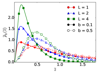
Figure 1: Salt free polymer density confined in the upper $\widetilde{z}>0$ half plane by a charged wall at $\widetilde{z}=0$ for different polymer lengths $L$ and monomer lengths $b$. The solid (filled) curves represent monomer length $b=0.1$ and dashed (unfilled) curves represent monomer length $b=0.5$.

In the SC regime, equation (15) says that the zeroth order term of the density distribution is the single polymer density of GPEs in an external potential of the wall potential $\widetilde{u}(\widetilde{z})$. We use a procedure developed by Edwards Doi and Edwards (1988); Edwards (1965) to calculate the single polymer density by partial differential equations. The zeroth order density distribution is then

$$\widetilde{\rho}_{0}(\widetilde{z}) =\Lambda_{0}\widetilde{\Omega}(\widetilde{z})\int_{0}^{N}dsq(\widetilde{z},N-s;\widetilde{u})q(\widetilde{z},s;\widetilde{u}),$$ (18)

where the function $q(\widetilde{z},s)$ satisfies the following differential equation

$$\left(\frac{\partial}{\partial N}-\frac{b^{2}}{6}\frac{\partial^{2}}{\partial\widetilde{z}^{2}}+\widetilde{u}(\widetilde{z})\right)q(\widetilde{z};N)=0.$$ (19)

The function $q(\widetilde{z};N)$ satisfies the constraint $q(\widetilde{z};0)=1$. Since the walls are impenetrable the density of the GPEs and hence $q(\widetilde{z};N)$ vanishes on the wall surface, $q(0;N)=0$. The ion confinement function $\widetilde{\Omega}(\widetilde{z})$ in equation (18) for a single wall confinement is

$$\widetilde{\Omega}(\widetilde{z}) =1\hskip 5.69054pt\text{for }0<\widetilde{z},$$

$$=0\hskip 5.69054pt\text{for }\widetilde{z}<0.$$ (20)

$\Lambda_{0}$ in equation (18) is obtained from the charge neutrality condition Netz (2001)

$$\int d\widetilde{z}\widetilde{\rho}_{0}(\widetilde{z})=1,$$ (21)

from which we obtain the zeroth order density as

$$\widetilde{\rho}_{0}(\widetilde{z}) =\frac{\widetilde{\Omega}(\widetilde{z})\int_{0}^{N}dsq(\widetilde{z},N-s;\widetilde{u})q(\widetilde{z},s;\widetilde{u})}{\int d\widetilde{z}\widetilde{\Omega}(\widetilde{z})\int_{0}^{N}dsq(\widetilde{z},N-s;\widetilde{u})q(\widetilde{z},s;\widetilde{u})}$$ (22)

The density profile is that of adsorption when the density of the PEs in the vicinity of the wall is higher than their bulk density. Figure 1 shows that the density profile is that of adsorption for lengths of the GPEs $L=1$, $2$ and $4$ for monomer lengths $b=0.1$ and $0.5$. Since the longer chains have higher charge, they have higher electrostatic attractions with the oppositely charged wall. Hence they are more strongly adsorbed into the wall and their density distribution falls sharply compared to the shorter chains. GPEs with longer monomer lengths $b$, but having the same number of monomers $L$ and charge, have lower surface charge density. Their attractions with the wall are weaker and they distribute further from the wall. Also the orientational degrees of freedom of chains with the same number of monomer but with larger monomer size is severely restricted near the wall. Therefore it is more entropically favorable for them to be situated farther from the wall. We look at this adsorption behavior of GPEs in detail and introduce a quantity called polymer fraction to quantify the adsorption phenomena in the next Section.

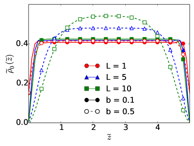
Figure 2: Salt free polymer density confined between two charged walls with an inter-wall separation of $\widetilde{d}$ for different polymer lengths $L$ and monomer lengths $b$. The solid (filled) curves represent monomer length $b=0.1$ and dashed (unfilled) curves represent monomer length $b=0.5$.

III.2 Two charged walls

For GPEs confined between two charged plates located at $\widetilde{z}=0$ and $\widetilde{z}=\widetilde{d}$ respectively, the rescaled wall potential in this case is Netz (2001)

$$\widetilde{u}(\widetilde{z})=0,$$ (23)

where the reference point $\widetilde{\mathbf{x}_{0}}$ in the equation (8) is chosen to lie at the midplane between the two walls.

The zeroth order density profile is given by the same equation (18) except $q$ now satisfies the following differential equation

$$\left(\frac{\partial}{\partial N}-\frac{b^{2}}{6}\frac{\partial^{2}}{\partial\widetilde{z}^{2}}\right)q(\widetilde{z};N)=0,$$ (24)

with impenetrable boundary conditions at the walls $q(0;N)=0$ and $q(\widetilde{d};N)=0$. Also the ion confinement function $\widetilde{\Omega}(\widetilde{z})$ is modified to

$$\widetilde{\Omega}(\widetilde{z}) =1\hskip 5.69054pt\text{for }0<\widetilde{z}<\widetilde{d},$$

$$=0\hskip 5.69054pt\text{otherwise }.$$ (25)

Figure 2 shows that the density profile of the GPEs is that of depletion for all lengths of the chains. Due to weaker attractions with the wall the chains with longer monomers having smaller charge density move towards the midplane between the two walls. Also the chains with smaller monomers have strong repulsions which makes it more energetically favorable for them to be spread nearly uniformly between the walls.

IV Salt

To study the effect of the salt on our system, we use a screened potential

$$\widetilde{v}(|\widetilde{\mathbf{x}}-\widetilde{\mathbf{x}}^{\prime}|)=\exp\left(-\kappa|\widetilde{\mathbf{x}}-\widetilde{\mathbf{x}}^{\prime}|\right)/|\widetilde{\mathbf{x}}-\widetilde{\mathbf{x}}^{\prime}|,$$ (26)

that depends on the salt concentration $c$ through the screening length. The screening length $\kappa^{-1}=(8\pi l_{B}c)^{-1/2}$ is made dimensionless by scaling with the Guoy-Chapman-like length $\mu$ and can be expressed as a function of the dimensionless salt density $\widetilde{c}=c\mu^{3}$ by

$$\widetilde{\kappa}=\kappa\mu=(8\pi\Xi\widetilde{c})^{1/2}.$$ (27)

IV.1 One wall

Plugging equation (26) in equation (8) and by choosing the reference point on the wall $\widetilde{\mathbf{x}}_{0}=0$, the wall potential becomes

$$\widetilde{u}(\widetilde{z}) =-\int_{0}^{\infty}\frac{\exp(-\widetilde{\kappa}\sqrt{\rho^{2}+\widetilde{z}^{2}})}{\sqrt{\rho^{2}+\widetilde{z}^{2}}}\rho d\rho+\int_{0}^{\infty}\exp(-\widetilde{\kappa}\rho)d\rho$$

$$=\frac{1}{\kappa}\left(1-\exp(-\widetilde{\kappa}\widetilde{z})\right).$$ (28)

When there is no screening $\widetilde{\kappa}=0$, we recover the wall potential $\widetilde{u}(\widetilde{z})$ in equation (17).

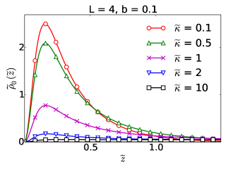
(a)

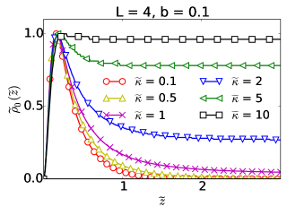
(b)

Figure 3: (a) Polymer density near a charged wall for various inverse screening lengths $\kappa$. (b) Polymer densities in (a) scaled by their corresponding maximum values.

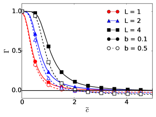
(a)

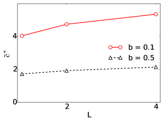
(b)

Figure 4: (a) The fraction of polymers adsorbed into the wall $\Gamma$ vs the salt concentrations $\widetilde{c}$ for various number of monomers $L$ and monomer lengths $b$. At low salt concentrations $\Gamma>0$ showing adsorption while at large salt concentration $\Gamma<0$ which signals depletion. The solid (filled) curves represent monomer length $b=0.1$ and dashed (unfilled) curves represent monomer length $b=0.5$. (b) The critical salt concentration $\widetilde{c}^{\ast}$ for adsorption-depletion transition vs the polymer lengths $L$ and monomer lengths $b$.

Figure 3 shows the density of GPEs in the presence of salt. Increasing $\kappa$ decreases the electrostatic correlations between the wall and the counterions. This decreases the distribution of polymers near the wall. Figure 3-(b) depicts the density profile as in Figure 3-(a) but each curve is scaled with its maximum value. On increasing the screening the bulk polymer develops a non-zero value. The plot also shows the transition of the density distribution from adsorption, when the density near the wall is much higher than the bulk density, to depletion, when the density is almost flat. At low screening the strong attractions with the walls cause almost all the polymers to be adsorbed into the wall and the bulk polymer concentration is zero. On increasing the screening the attractions decreases and more and more GPEs leave the wall and move to the bulk causing depletion. We can make a more accurate estimate of the transition by measuring the total amount of polyelectrolytes in the adsorbed layer Shafir et al. (2003) by

$$\Gamma=\int_{0}^{\infty}d\widetilde{z}\left(\widetilde{\rho}_{0}(\widetilde{z})-\widetilde{\rho}_{0}^{b}\right),$$ (29)

where $\widetilde{\rho}_{0}^{b}=\widetilde{\rho}_{0}(\widetilde{z}=\infty)$ is the bulk density of the GPEs. In the adsorption region $\Gamma$ is positive while in the depletion region $\Gamma$ is negative. Thus $\Gamma=0$ would signify the transition from adsorption to depletion as shown in Figure 4-(a) by varying the salt concentration $\widetilde{c}$. $\Gamma=1$ at low salt concentrations implies almost all the polymers are adsorbed into the wall. On increasing the salt, the entropic forces takes over the electrostatic correlations and the polymers spread away from the wall. Figure 4-(b) plots the critical salt concentration $\widetilde{c}^{\ast}$ when the polymer density profile changes from adsorption to depletion, $\Gamma=0$. Longer chains have stronger electrostatic attractions with the wall and hence their transition from the adsorption to depletion transition occurs at a higher salt concentration as seen from the same Figure. Chains with shorter monomer lengths have higher charge densities and hence stronger electrostatic correlations and need higher salt screening to overcome them. As noted earlier chains with longer monomers have much less orientational freedom closer to the wall, hence it is easier to salt them out.

IV.2 Two wall

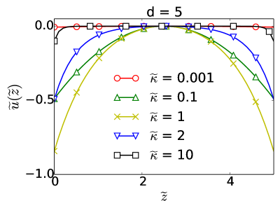
Figure 5: The dependence of the wall potential $\widetilde{u}(\widetilde{z})$ on the inverse screening length $\kappa$ with the inter-wall distance is $\widetilde{d}=5$.

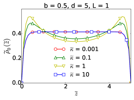
(a)

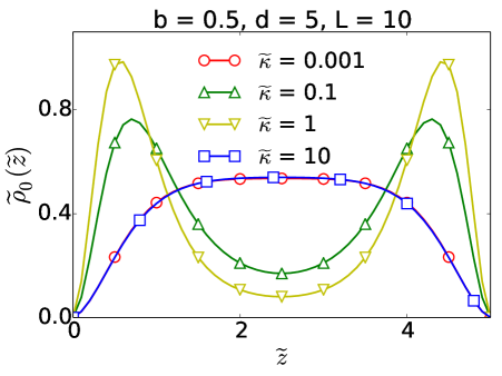
(b)

Figure 6: Polymer densities vs the inverse screening lengths $\kappa$ with inter-wall separation of $\widetilde{d}=5$ for polymer lengths (a) $L=1$ and (b) $L=10$.

(a)

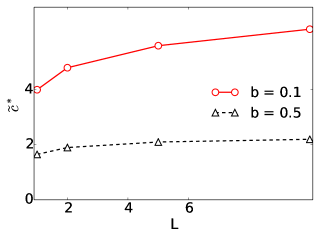
(b)

Figure 7: (a) The polymer adsorption fraction showing the depletion-adsorption-depletion transitions on increasing the salt concentrations $\widetilde{c}$. The solid (filled) curves represent monomer length $b=0.1$ and dashed (unfilled) curves represent monomer length $b=0.5$. (b) The dependence of the critical salt concentration on the polymer lengths $L$.

When there are two walls, the wall potential is obtained from equation (28) for the one wall case or from equations (8) and (26) with the reference point $\widetilde{\mathbf{x}}_{0}$ at the midplane between the two walls

$$\widetilde{u}(\widetilde{z})=\frac{1}{\kappa}\left(2\exp(-\kappa\widetilde{d}/2)-\exp(-\kappa\widetilde{z})-\exp(-\kappa|\widetilde{d}-\widetilde{z}|)\right).$$ (30)

We plot the wall potential $\widetilde{u}(\widetilde{z})$ in Figure 5 for various values of the screening parameter $\widetilde{\kappa}$ for the inter-wall separation of $\widetilde{d}=5$. When the salt concentration is zero or $\widetilde{\kappa}\rightarrow 0$, $\widetilde{u}(\widetilde{z})=0$ as in equation (23). When salt concentration $\widetilde{c}$ and hence $\widetilde{\kappa}$ is large, again we see from the Figure that $\widetilde{u}(\widetilde{z})\approx 0$ especially when the walls are further apart. When there is no screening the electric fields of the walls are equal and opposite and cancel each other because of the planar nature of the walls. In the other limit of very high screening the potential is extremely short ranged and the potential is zero everywhere except very close to the walls. Thus effectively in the two limits the wall potential has the same form. As a result the density profile of GPEs are almost similar at low and high values of the screening parameter in Figure 6 irrespective of the lengths of the polymers. Since longer chains have higher charges they are more clustered towards the wall as shown in the Figure. In Figure 7-(a) the polymer adsorption fraction shows a transition of the density profile from depletion in the salt free regime to adsorption due to the variation of the wall potential from the zero electric field Coulomb to screened Yukawa regime. On further increasing the salt, the system again undergoes a depletion transition. In Figure 7-(b) the critical salt concentration for the adsorption-depletion transition is shown for different lengths of the polymers. It shows that the longer chains needs higher salt concentration to screen out their electrostatic correlations.

V Conclusions and discussions

We have presented a theoretical formalism to describe highly charged Gaussian polymer in presence of a fixed charged distribution. Using polymer field theory we have developed the formalism closely following the strong coupling theory by Netz and his coworkers Netz (2001); Moreira and Netz (2001). We considered the confinement of the GPEs by oppositely charged impenetrable walls in the presence and absence of salt. In the presence of salt we consider the confinement by one and two charged walls and study the dependence of the density profile on the geometry of the chains and the salt concentration. At low salt concentration and for confinement by a single wall, the polymers are strongly adsorbed into the wall especially the longer chains since they have stronger electrostatic attractions with the wall. On further increasing the salt concentration the chains de-adsorb from the wall and their density distribution shows a depletion transition. The dependence of the critical salt concentration at the adsorption-depletion transition on the geometry of the polymers is discussed. For the confinement between two walls, the wall potential is zero when it is salt-free and almost zero when there is high salt concentration. When there is no salt the electric fields due to the two plates are equal and opposite and they cancel each other. When there is large amount of salt in the solution the screening is strong and the potential is zero except very close to the walls. Thus in the two limits there are depletion and in the intermediate regime there is adsorption.

Our analysis is however valid for very strong coupling $\Xi>>1$, because of which we consider only the zeroth order term of the density. The single particle description is appropriate when the polymer is shorter then the Wigner cell. This analysis would be true for the layer closest to the walls, but for the polymers located off the condensed layer the higher order terms, which have the excluded volume and the two polymer electrostatic interaction effects, have to be taken into consideration. The intermediate coupling regime which occurs in most real systems. Most biopolymers also have finite bending rigidity and semi-flexible polymers not Gaussian polymers are a better description for them. Extension of this analysis to semiflexible polymers will be done in a subsequent paper.

References

- Luger et al. (1997) K. Luger, A. W. Mäder, R. K. Richmond, D. F. Sargent, and T. J. Richmond, Nature 389, 251 (1997).
- Cherstvy (2009) A. Cherstvy, The Journal of Physical Chemistry B 113, 4242 (2009).
- Belyi and Muthukumar (2006) V. A. Belyi and M. Muthukumar, Proceedings of the National Academy of Sciences 103, 17174 (2006).
- Forrey and Muthukumar (2009) C. Forrey and M. Muthukumar, The Journal of chemical physics 131, 105101 (2009).
- Jho et al. (2010) Y. Jho, E. Zhulina, M. Kim, and P. Pincus, Biophysical journal 99, 2387 (2010).
- Caruso et al. (1999) F. Caruso, H. Lichtenfeld, E. Donath, and H. Möhwald, Macromolecules 32, 2317 (1999).
- Baumgärtner and Muthukumar (1991) A. Baumgärtner and M. Muthukumar, The Journal of chemical physics 94, 4062 (1991).
- Von Goeler and Muthukumar (1994) F. Von Goeler and M. Muthukumar, The Journal of chemical physics 100, 7796 (1994).
- Linse (1996) P. Linse, Macromolecules 29, 326 (1996).
- Shafir et al. (2003) A. Shafir, D. Andelman, and R. R. Netz, The Journal of chemical physics 119, 2355 (2003).
- Winkler and Cherstvy (2006) R. G. Winkler and A. G. Cherstvy, Physical review letters 96, 066103 (2006).
- Man et al. (2008) X. Man, S. Yang, D. Yan, and A.-C. Shi, Macromolecules 41, 5451 (2008).
- Ličer and Podgornik (2010) M. Ličer and R. Podgornik, Journal of Physics: Condensed Matter 22, 414102 (2010).
- Wang et al. (2011) Z. Wang, B. Li, D. Ding, and Q. Wang, Macromolecules 44, 8607 (2011).
- Cherstvy and Winkler (2012) A. Cherstvy and R. Winkler, The Journal of Physical Chemistry B 116, 9838 (2012).
- De Gennes (1979) P.-G. De Gennes, Scaling concepts in polymer physics (Cornell university press, 1979).
- Podgornik (1990) R. Podgornik, Chemical Physics Letters 174, 191 (1990).
- Chodanowski and Stoll (2001) P. Chodanowski and S. Stoll, The Journal of Chemical Physics 115, 4951 (2001).
- Kong and Muthukumar (1998) C. Kong and M. Muthukumar, The Journal of chemical physics 109, 1522 (1998).
- Welch and Muthukumar (2000) P. Welch and M. Muthukumar, Macromolecules 33, 6159 (2000).
- Messina et al. (2004) R. Messina, C. Holm, and K. Kremer, Journal of Polymer Science part B: polymer physics 42, 3557 (2004).
- Ulrich et al. (2005) S. Ulrich, A. Laguecir, and S. Stoll, Macromolecules 38, 8939 (2005).
- Forsman (2012) J. Forsman, Langmuir 28, 5138 (2012).
- Xie et al. (2013) F. Xie, T. Nylander, L. Piculell, S. Utsel, L. Wågberg, T. Åkesson, and J. Forsman, Langmuir 29, 12421 (2013).
- Stoll and Chodanowski (2002) S. Stoll and P. Chodanowski, Macromolecules 35, 9556 (2002).
- Källrot and Linse (2010) N. Källrot and P. Linse, The Journal of Physical Chemistry B 114, 3741 (2010).
- Ulrich et al. (2006) S. Ulrich, M. Seijo, and S. Stoll, Current opinion in colloid & interface science 11, 268 (2006).
- Cao et al. (2011) Q. Cao, C. Zuo, Y. Ma, L. Li, and Z. Zhang, Soft Matter 7, 506 (2011).
- Carnal and Stoll (2011) F. Carnal and S. Stoll, The Journal of Physical Chemistry B 115, 12007 (2011).
- Cerdà et al. (2009) J. J. Cerdà, B. Qiao, and C. Holm, Soft Matter 5, 4412 (2009).
- Jeong et al. (2014) S. Jeong, X. Zhou, E. B. Zhulina, and Y. Jho, Israel Journal of Chemistry (2014).
- McQuigg et al. (1992) D. W. McQuigg, J. I. Kaplan, and P. L. Dubin, The Journal of Physical Chemistry 96, 1973 (1992).
- Feng et al. (2001) X. Feng, P. Dubin, H. Zhang, G. Kirton, P. Bahadur, and J. Parotte, Macromolecules 34, 6373 (2001).
- Kayitmazer et al. (2005) A. Kayitmazer, D. Shaw, and P. Dubin, Macromolecules 38, 5198 (2005).
- Cherstvy and Winkler (2011) A. Cherstvy and R. Winkler, Physical Chemistry Chemical Physics 13, 11686 (2011).
- Châtellier and Joanny (1996) X. Châtellier and J.-F. Joanny, Journal de Physique II 6, 1669 (1996).
- Joanny (1999) J. Joanny, The European Physical Journal B-Condensed Matter and Complex Systems 9, 117 (1999).
- Wiegel (1977) F. Wiegel, Journal of Physics A: Mathematical and General 10, 299 (1977).
- Muthukumar (1987) M. Muthukumar, The Journal of chemical physics 86, 7230 (1987).
- Borukhov et al. (1998) I. Borukhov, D. Andelman, and H. Orland, Macromolecules 31, 1665 (1998).
- Borukhov et al. (1995) I. Borukhov, D. Andelman, and H. Orland, EPL (Europhysics Letters) 32, 499 (1995).
- Borisov et al. (1994) O. Borisov, E. Zhulina, and T. Birshtein, Journal de Physique II 4, 913 (1994).
- Dobrynin et al. (2001) A. V. Dobrynin, A. Deshkovski, and M. Rubinstein, Macromolecules 34, 3421 (2001).
- Dobrynin et al. (2000) A. V. Dobrynin, A. Deshkovski, and M. Rubinstein, Physical review letters 84, 3101 (2000).
- Dobrynin and Rubinstein (2005) A. V. Dobrynin and M. Rubinstein, Progress in Polymer Science 30, 1049 (2005).
- Netz and Joanny (1999) R. R. Netz and J.-F. Joanny, Macromolecules 32, 9013 (1999).
- Netz and Andelman (2003) R. R. Netz and D. Andelman, Physics Reports 380, 1 (2003).
- Edwards (1965) S. F. Edwards, Proceedings of the Physical Society 85, 613 (1965).
- Shklovskii (1999a) B. I. Shklovskii, Physical review letters 82, 3268 (1999a).
- Shklovskii (1999b) B. I. Shklovskii, Physical Review E 60, 5802 (1999b).
- Perel and Shklovskii (1999) V. Perel and B. Shklovskii, Physica A: Statistical Mechanics and its Applications 274, 446 (1999).
- Grosberg et al. (2002) A. Y. Grosberg, T. T. Nguyen, and B. I. Shklovskii, Rev. Mod. Phys. 74, 329 (2002).
- Netz (2001) R. Netz, The European Physical Journal E 5, 557 (2001), ISSN 1292-8941.
- Moreira and Netz (2001) A. G. Moreira and R. R. Netz, Physical review letters 87, 078301 (2001).
- Kanduč et al. (2009) M. Kanduč, A. Naji, Y. Jho, P. A. Pincus, and R. Podgornik, Journal of Physics: Condensed Matter 21, 424103 (2009).
- Naji et al. (2013) A. Naji, M. Kanduč, J. Forsman, and R. Podgornik, The Journal of chemical physics 139, 150901 (2013).
- Levin (2002) Y. Levin, Reports on progress in physics 65, 1577 (2002).
- Naji (2005) A. Naji, Ph.D. thesis, lmu (2005).
- Boroudjerdi et al. (2005) H. Boroudjerdi, Y.-W. Kim, A. Naji, R. Netz, X. Schlagberger, and A. Serr, Physics reports 416, 129 (2005).
- Bohinc et al. (2012) K. Bohinc, J. M. Grime, and L. Lue, Soft Matter 8, 5679 (2012).
- Kim et al. (2008) Y. W. Kim, J. Yi, and P. Pincus, Physical review letters 101, 208305 (2008).
- Dutta and Jho (2015) S. Dutta and Y. S. Jho, Submitted (2015), URL http://arxiv.org/abs/1511.03388.
- Šamaj and Trizac (2011a) L. Šamaj and E. Trizac, Phys. Rev. E 84, 041401 (2011a).
- Šamaj and Trizac (2011b) L. Šamaj and E. Trizac, Phys. Rev. Lett. 106, 078301 (2011b).
- Hatlo and Lue (2010) M. M. Hatlo and L. Lue, Europhys. Lett. 89, 25002 (2010).
- Fredrickson (2006) G. H. Fredrickson, The equilibrium theory of inhomogeneous polymers (Clarendon, 2006).
- Doi and Edwards (1988) M. Doi and S. F. Edwards, The theory of polymer dynamics, vol. 73 (oxford university press, 1988).