Families of Orthogonal Schrödinger cat-like-states

Abstract

We analyze condition of orthogonality between optical Schrödinger cat-like-states constructed as superposition of two coherent states. We show that the orthogonality condition leads to quantization of values of a naturally emerging symplectic form, while values of the corresponding metric form are continuous. A complete analytical solution of the problem is presented.

I Introduction

A set of nonorthogonal wave functions that naturally appear in the description of quantum harmonic oscillator was known from the beginnings of quantum theory. It was firstly mentioned by Schrodinger’s Schrodinger in 1926 and analyzed later in von Neumann’s Mathematische Grundlagen der Quantenmechanik vonNeumann . The name ‘coherent states’ was proposed by Glauber in the context of description of coherent laser beams in 1963 Glauber . Since then, formalism of coherent states often serves as a language of quantum optics – especially in its phase space representation. Not without reason: as the ‘most classical from quantum states’ coherent states match classical intuitions, when at the same time superposition of coherent states are nonclassical enough to reveal purely quantum effects. As a typical example usually serves a superposition of two coherent states, a so-called Schrödinger-cat-like state.

Superpositions of coherent states have been studied in the contexts of quantum error correction Cochrane , quantum teleportation Enk , and quantum computation Kim ; Glancy . The majority of these applications exploit the fact that a cat-like state split on a beamsplitter produces an entangled state. There are many theoretical proposals of generation of such superposition and a number of experimental realizations ourj ; ourj2 ; Takahashi . I believe that many from proposals mentioned above could benefit from the use of additional fact that, unlike single coherent states, their superpositions form families of orthogonal states. This paper presents an analysis showing that the scalar product between superpositions of coherent states can be exactly zero – not just reaches ‘close to zero’ values, as it is the case when single coherent states are used, e.g., as logical qubits.

Coherent states minimize uncertainty relation; they are connected to the eigenvectors of a quantum harmonic oscillator, $|m\rangle_{\!{}_{osc}}$, by the formula

$$|\alpha\rangle=e^{\frac{-|\alpha|^{2}}{2}}\sum_{m=0}^{\infty}\frac{\alpha^{m}}{\sqrt{m!}}|m\rangle_{\!{}_{osc}},$$ (1)

and they form an over-complete (but not orthogonal) basis. Average number of photons in (1) is equal to $|\alpha|^{2}$. Although two coherent states are never orthogonal to each other, the scalar product between them vanishes exponentially with distance $\big{|}\langle\beta|\alpha\rangle\big{|}^{2}\!=\exp({-|\alpha-\beta|^{2}})$, which for large enough values of $|\alpha|$ allows to treat a sum

$${\mathcal{K}}_{\!{}_{\varphi}}\!(\alpha):=|\alpha\rangle+e^{i\varphi}|-\alpha\rangle\,,$$ (2)

as a close optical analogue of the superposition of macroscopically distinguishable states from the Schrödinger’s gedanken experiment Schrodinger_cat . For small values of $|\alpha|$ (and significant overlap between the states) such superpositions are known as Schrödinger kitten. Because of an omitted normalization factor, we shall refer to ${\mathcal{K}}_{\!{}_{\varphi}}(\alpha)$ as to vector rather then a state. For $\varphi=0$ and $\varphi=\pi$, vector ${\mathcal{K}}_{\!{}_{\varphi}}(\alpha)$ corresponds respectively to even and odd coherent states introduced in Hillery . Note, also, that the phase in (2) is not equivalent the one studied in Kien where superpositions of the form $|\alpha e^{i\phi}\rangle+|\alpha e^{-i\phi}\rangle$ were considered.

The Wigner function Wigner of a cat-like state is often used to illustrate how decoherence affects quantum superpositions BuzekKnight ; Zurek_decoh . In this phase space representation it is clearly seen that addition of a noise to the system destroys the interference terms, while Gaussian peaks corresponding to $|\alpha\rangle$ or $|-\alpha\rangle$ remain unaffected. It was shown, that the coherent states are especially robust to decoherence, thus, can serve as the ‘pointer’ states Zurek_decoh . More information about mathematical properties of coherent states and their generalizations can be found in Perelomov ; Gazeau . A short list of symbols used in this paper is presented in Appendix A.

II Superposition of coherent states

II.1 A coherent state is orthogonal to …

We have emphasized that coherent states are not orthogonal to each other. It does not mean that also superpositions of coherent states always have non-zero scalar product. The most obvious example of a vanishing overlap between Schrödinger-cat-like states is obtained via change of a relative phase: vector ${\mathcal{K}}_{\pi}(\alpha)$ is orthogonal to ${\mathcal{K}}_{\scriptscriptstyle{0}}(\alpha)$. This fact is easily proved, one just have to realize the difference in the parity of the corresponding states. Substituting (1) into ${\mathcal{K}}_{\scriptscriptstyle{0}}(\alpha)$ and ${\mathcal{K}}_{\pi}(\alpha)$ one sees that the former consists only of even number states, while the later only of odd number states Hillery . The same argument proves that ${\mathcal{K}}_{\pi}(\alpha)$ and ${\mathcal{K}}_{\scriptscriptstyle{0}}(\beta)$ are always orthogonal and that the vacuum state $|0\rangle$ is orthogonal to ${\mathcal{K}}_{\!\pi}(\alpha)$ for any $\alpha$. Another example is a class of vectors orthogonal to ${\mathcal{K}}_{\scriptscriptstyle{0}}(d)$, $d\mathrel{\raisebox{1.0pt}{$\!{\scriptstyle\in}\!$}}\mathbb{R}^{\times},$ defined as

$${\mathcal{J}}\!(d,\delta_{k}):=|d+i\delta_{k}\rangle+|-d+i\delta_{k}\rangle\,,$$

where $\delta_{k}=\pi(2k+1)/(2d)$ and $k\mathrel{\raisebox{1.0pt}{$\!{\scriptstyle\in}\!$}}\mathbb{Z}$. Each value of $\delta_{k}$ corresponds to a shift in momentum that makes ${\mathcal{K}}_{\scriptscriptstyle{0}}(d)$ and ${\mathcal{J}}\!(d,\delta_{k})$ orthogonal to each other frogTorun .

One might wonder if a superposition ${\mathcal{K}}_{\varphi}(\alpha)$ could be orthogonal to a single coherent state different then $|0\rangle$. The answer is yes: for example an overlap of vector $|\alpha\rangle$ for any set but nonzero real $\alpha$, and ${\mathcal{K}}_{\scriptscriptstyle{0}}(\beta_{n})$ for

$$\beta_{n}=i\pi(n+{1}/{2})/\alpha,$$ (3)

vanishes for all natural $n$, i.e.,

$$\langle\alpha|{\mathcal{K}}_{\scriptscriptstyle{0}}\!{\textstyle\big{(}i\pi(n+{1}/{2})/\alpha\big{)}}\rangle=0\qquad\mathrm{for}\;\alpha\mathrel{\raisebox{1.0pt}{$\!{\scriptstyle\in}\!$}}\mathbb{R}^{\times},\;n\mathrel{\raisebox{1.0pt}{$\!{\scriptstyle\in}\!$}}\mathbb{N}.$$

For a set value of $n$, the smaller $|\alpha|$ the further apart are $|\beta_{n}\rangle$ and $|-\beta_{n}\rangle$; for a set $\alpha$, the amplitude $|\beta_{n}|$ increases with $n$.

To illustrate examples used, we will either plot the corresponding Husimi functions Husimi or just represent a coherent state $|\alpha\rangle$ as a circle of radii $1/\sqrt{2}\,$ centered at point $(\mathrm{Re}(\alpha),\mathrm{Im}(\alpha))$. For a given density matrix $\hat{\varrho}$, Husimi function is defined as

$$\mathrm{Q}_{\hat{\varrho}}(\gamma)=Tr[\hat{\varrho}|\gamma\rangle\langle\gamma|].$$ (4)

Figure 1 shows Husimi functions corresponding to cat-like superpositions orthogonal to coherent state $|5\rangle$.

 

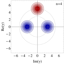
a)   b)

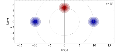
Figure 1: Phase space Husimi representation of coherent state $|5\rangle$ (plotted in red) and orthogonal to it cat-like superposition ${\mathcal{K}}_{\scriptscriptstyle{0}}(\beta_{n})$ (plotted in blue). Amplitudes of orthogonal states take on discrete values and increase with n. Blue circles in plots a) and b) correspond to vectors ${\mathcal{K}}_{\scriptscriptstyle{0}}(i\pi(0.9))$ and ${\mathcal{K}}_{\scriptscriptstyle{0}}(i\pi(3.1))$ obtained from (3) for $n=4$ or n=15, respectively.

 

The first example, depicted in Fig. 1.a, corresponds to $n=4$ and vector ${\mathcal{K}}_{\scriptscriptstyle{0}}(i\pi(0.9))$. The second, Fig. 1.b, was calculated for $n=15$ and corresponds to vector ${\mathcal{K}}_{\scriptscriptstyle{0}}(i\pi(3.1))$. In both figures, Husimi function of state $|5\rangle$ is plotted in red, and Husimi functions of the orthogonal vectors ${\mathcal{K}}_{\scriptscriptstyle{0}}(\beta_{n})$ are plotted in blue. Dashed circles of radii $5$ and $|\beta_{n}|$ denote phase-space trajectories of free evolution of coherent states $|5\rangle$, $|\beta_{n}\rangle$. Note, that in respect to typical notation position ($\sqrt{2}\mathrm{Re}(\gamma)$) and momentum ($\sqrt{2}\mathrm{Im}(\gamma)$) axes in these plots are exchanged.

II.2 Even and odd coherent states

II.2.1 Orthogonality between even cats

Consider a superposition of two coherent states of form ${\mathcal{K}}_{\scriptscriptstyle{0}}\!(\alpha)$, Eq. (2). It can be proved that:

Fact 1 For any $\alpha,\beta\mathrel{\raisebox{1.5pt}{$\!{\scriptstyle\in}\!$}}\mathbb{C}^{\times}$, the following conditions are equivalent:
$1^{\circ}\quad$ $\langle{\mathcal{K}}_{\scriptscriptstyle{0}}(\beta)|{\mathcal{K}}_{\scriptscriptstyle{0}}(\alpha)\rangle=0\,.$
$2^{\circ}\quad$ There exists $n\mathrel{\raisebox{1.0pt}{$\!{\scriptstyle\in}\!$}}\mathbb{N}$, such that

$${\mathcal{K}}_{\scriptscriptstyle{0}}(\beta)={\mathcal{K}}_{\scriptscriptstyle{0}}(\beta_{n}):=|-i\pi(2n+1)/(2\alpha^{*})\rangle+|i\pi(2n+1)/(2\alpha^{*})\rangle\,.$$ (5)

It is seen, that for a given non-zero $\alpha$ there exists a whole class of solutions of $1^{\circ}\,$ parametrized by natural number $n$, each rotated in phase space by $\pi/2$ in respect to ${\mathcal{K}}_{\scriptscriptstyle{0}}(\alpha)$. Figure 2 shows examples of Husimi functions calculated for pairs of orthogonal vectors ${\mathcal{K}}_{\scriptscriptstyle{0}}(\alpha)$ (plotted in green) and ${\mathcal{K}}_{\scriptscriptstyle{0}}(\beta_{n})$ (plotted in blue), for parameters $\alpha=4+i8$ and $\beta_{n}$

 

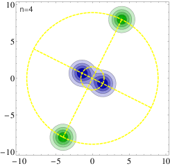
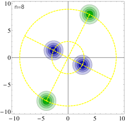
a) $\mathrm{Im}(\gamma)$   b)  c)

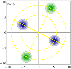
$\mathrm{Re}(\gamma)$                                      $\mathrm{Re}(\gamma)$                                    $\mathrm{Re}(\gamma)$  

Figure 2: Husimi functions corresponding to the pairs of orthogonal Schrodinger-like-cat superpositions. Initial cat ${\mathcal{K}}_{\scriptscriptstyle{0}}\!(4+i8)$ is depicted in green. Plotted in blue are Husimi functions corresponding to ${\mathcal{K}}_{\scriptscriptstyle{0}}\!(\beta_{n})$ from (5), for a) n=4; b) n=8; c) n=16, respectively.

corresponding to $n=4$, $n=8$, $n=16$, respectively. Comparison between Figs. 2 a), b) and c) reveals how change of $n$ changes distance between states forming superposition (5). In general, separation $2|\beta_{n}|$ is different then $2|\alpha|$ for every value of parameter $n$. Below we consider a very special case when the distances between states forming orthogonal superpositions ${\mathcal{K}}_{\scriptscriptstyle{0}}(\alpha)$ and ${\mathcal{K}}_{\scriptscriptstyle{0}}(\beta)$ are equal.

Fact 2 For $\alpha,\beta\mathrel{\raisebox{1.5pt}{$\!{\scriptstyle\in}\!$}}\mathbb{C}^{\times}$ such that $\langle{\mathcal{K}}_{\scriptscriptstyle{0}}(\alpha)|{\mathcal{K}}_{\scriptscriptstyle{0}}(\beta)\rangle=0$ the following conditions are equivalent:
$1^{\circ}\quad$ $|\alpha|=|\beta|$ .
$2^{\circ}\quad$ There exists $n\mathrel{\raisebox{1.0pt}{$\!{\scriptstyle\in}\!$}}\mathbb{N}$ such that $|\alpha|=\sqrt{(n+1/2)\pi}\;.$

Example of two even cat superpositions with equal average number of photons is presented in Fig. 5.a). Dashed circles show the only possible values of $\alpha$ satisfying condition $2^{\circ}$ from Fact 2. Areas of bands between the subsequent circles are equal to $\pi^{2}$.

II.2.2 Orthogonality between odd cats

Similarly, one might consider two coherent states forming an ‘odd’ cat-like superposition ${\mathcal{K}}_{\scriptstyle{\pi}}\!(\alpha^{\prime})$ and prove the facts listed below:

Fact 3 For any $\alpha^{\prime},\beta^{\prime}\mathrel{\raisebox{1.5pt}{$\!{\scriptstyle\in}\!$}}\mathbb{C}^{\times}$, the following conditions are equivalent:
$1^{\circ}\quad$ $\langle{\mathcal{K}}_{\scriptstyle{\pi}}(\beta^{\prime})|{\mathcal{K}}_{\scriptstyle{\pi}}(\alpha^{\prime})\rangle=0\,.$
$2^{\circ}\quad$ There exists $n\mathrel{\raisebox{1.0pt}{$\!{\scriptstyle\in}\!$}}\mathbb{N}^{\times}$, such that ${\mathcal{K}}_{\scriptstyle{\pi}}(\beta^{\prime})={\mathcal{K}}_{\scriptstyle{\pi}}(\beta^{\prime}_{n}):=|-in\pi/\alpha^{\prime*}\rangle-|in\pi/\alpha^{\prime*}\rangle\,.$
(Note that, for $n=0$, the orthogonality condition holds, although it is reduced to a trivial case.)

Fact 4 For $\alpha^{\prime},\beta^{\prime}\mathrel{\raisebox{1.5pt}{$\!{\scriptstyle\in}\!$}}\mathbb{C}^{\times}$ such that $\langle{\mathcal{K}}_{\scriptstyle{\pi}}(\alpha^{\prime})|{\mathcal{K}}_{\scriptstyle{\pi}}(\beta^{\prime})\rangle=0$ the following conditions are equivalent:
$1^{\circ}\quad$ $|\alpha^{\prime}|=|\beta^{\prime}|$ .
$2^{\circ}\quad$ There exists $n\mathrel{\raisebox{1.0pt}{$\!{\scriptstyle\in}\!$}}\mathbb{N}^{\times}$ such that ${\textstyle|\alpha^{\prime}|=\sqrt{n\pi}}\;.$

Figure 3 shows a phase space representation of pair of orthogonal vectors ${\mathcal{K}}_{\scriptstyle{\pi}}(\alpha^{\prime}),{\mathcal{K}}_{\scriptstyle{\pi}}(\beta^{\prime})$ fulfilling condition $|\alpha^{\prime}|=|\beta^{\prime}|$. Black dashed lines denote other circles of radii of form $r_{n}=\sqrt{n\pi}.$ As before, areas of bands between the closest-neighbors circles are equal to $\pi^{2}$. There is a factor of $\sqrt{\pi}$ difference between these radii and those separating the subsequent Planck-Bohr-Sommerfeld bands Kien corresponding to number states in the semiclassical limit.

 

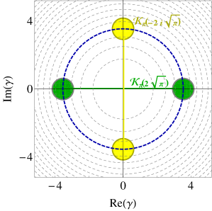
Figure 3: Phase space representation of a pair of orthogonal odd cats with the same average number of photons. Superposition ${\mathcal{K}}_{\pi}(\alpha^{\prime})\!=|\sqrt{4\pi}\rangle-|-\sqrt{4\pi}\rangle\,$ is plotted in green and the orthogonal superposition ${\mathcal{K}}_{\pi}(\beta^{\prime})\!=|-i\sqrt{4\pi}\rangle-|i\sqrt{4\pi}\rangle\,$ in yellow. Dashed lines denote circles of radii $r=\sqrt{n\pi}$ showing the only possible values such that $|\beta^{\prime}|=|\alpha^{\prime}|$ and $\langle{\mathcal{K}}_{\scriptstyle{\pi}}\!(\alpha^{\prime})|{\mathcal{K}}_{\scriptstyle{\pi}}\!(\beta^{\prime})\rangle=0$.

 

III Orthogonality between cat-like states – arbitrary relative phase

Let us consider a more general superpositions obtained for non-zero $\alpha$, $\beta$ and arbitrary relative phases $\varphi_{1},\varphi_{2}\mathrel{\raisebox{1.0pt}{$\!{\scriptstyle\in}\!$}}[0,2\pi[$. It can be shown that a condition

$$\big{|}\langle{\mathcal{K}}_{\varphi_{\!{}_{2}}}\!(\beta)|{\mathcal{K}}_{\varphi_{\!{}_{1}}}\!(\alpha)\rangle\big{|}^{2}=0\;$$ (6)

is equivalent to equation

$$e^{2\mathrm{Re}(\alpha\beta^{*})}\!\cos^{2}\!\!\big{(}{\textstyle{\frac{\varphi_{\!{}_{2}}-\varphi_{\!{}_{1}}}{2}}}\big{)}\!+\!e^{-2\mathrm{Re}(\alpha\beta^{*})}\!\cos^{2}\!\!\big{(}{\textstyle{\frac{\varphi_{\!{}_{2}}+\varphi_{\!{}_{1}}}{2}}}\big{)}\!=$$

$$=-2\cos\!\big{(}{\textstyle{\frac{\varphi_{\!{}_{2}}+\varphi_{\!{}_{1}}}{2}}}\big{)}\cos\!\big{(}{\textstyle{\frac{\varphi_{\!{}_{2}}-\varphi_{\!{}_{1}}}{2}}}\big{)}\cos\!\big{[}2\,\mathrm{Im}(\alpha\beta^{*})\big{]}.$$ (7)

In the paragraphs that follow, analysis od solutions of (7) is presented and dependance between parameters $\alpha,\,\beta,\,\varphi_{\!{}_{1}},\,\varphi_{\!{}_{2}}$ examined.

III.1 Case when $\cos({\scriptstyle{\frac{\varphi_{\!{}_{2}}+\varphi_{\!{}_{1}}}{2}}})\cos({\scriptstyle{\frac{\varphi_{\!{}_{2}}-\varphi_{\!{}_{1}}}{2}}})=0\,$

Note that when both $\cos({\scriptstyle{\frac{\varphi_{\!{}_{2}}+\varphi_{\!{}_{1}}}{2}}})=0$ and $\cos({\scriptstyle{\frac{\varphi_{\!{}_{2}}-\varphi_{\!{}_{1}}}{2}}})=0,$ (7) forms an identity. As a result, the scalar product (6) vanishes for any $\alpha$ and $\beta$. On a map presented in Fig. 4.a, phases $(\varphi_{\!{}_{1}},\varphi_{\!{}_{2}})\mathrel{\raisebox{1.0pt}{$\!{\scriptstyle\in}\!$}}\{(0,\pi),(\pi,0)\}$ corresponding to this case are illustrated as red circles. It is an example of orthogonality between odd and even cats, that occurs regardless of $\alpha$, $\beta$, which was already described in the beginning of Section II.1.

 

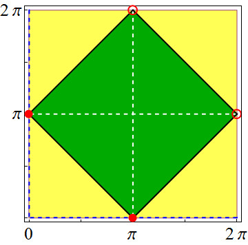
a)              b)

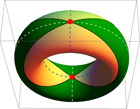
Figure 4: (a) Map of $(\varphi_{\!{}_{1}},\varphi_{\!{}_{2}})$ that organizes solutions of (7). Its periodic boundary conditions make it equivalent to a torus (b) showing that the green and yellow areas have the same topology. Red dots correspond to the case of odd and even cats which are orthogonal to each other for all values of $\alpha$, $\beta$. Dashed white and dashed blue lines correspond to cases when $\mathrm{Re}(\alpha\beta^{*})=0$ and one of the phases is equal to 0 or $\pi$ while the second is arbitrary. Values of $\varphi_{\!{}_{1}},\varphi_{\!{}_{2}}$ for which $\cos({\scriptstyle{\frac{\varphi_{\!{}_{2}}-\varphi_{\!{}_{1}}}{2}}})/\cos({\scriptstyle{\frac{\varphi_{\!{}_{2}}+\varphi_{\!{}_{1}}}{2}}})<0$ are plotted as a green inscribed square. Its black edges (open segments) denote the values for which only one of these cosines vanishes, and there are no solutions of (7). The remaining yellow triangles denote these $\varphi_{\!{}_{1}},\varphi_{\!{}_{2}}$ for which $\cos({\scriptstyle{\frac{\varphi_{\!{}_{2}}-\varphi_{\!{}_{1}}}{2}}})/\cos({\scriptstyle{\frac{\varphi_{\!{}_{2}}+\varphi_{\!{}_{1}}}{2}}})>0$. For angles forming open green and yellow areas there are always unambiguous solutions of (7).

 

Quite the opposite is the case when $\cos({\scriptstyle{\frac{\varphi_{\!{}_{2}}+\varphi_{\!{}_{1}}}{2}}})\cos({\scriptstyle{\frac{\varphi_{\!{}_{2}}-\varphi_{\!{}_{1}}}{2}}})=0\,$ but either $\cos({\scriptstyle{\frac{\varphi_{\!{}_{2}}-\varphi_{\!{}_{1}}}{2}}})\neq 0$ or $\cos({\scriptstyle{\frac{\varphi_{\!{}_{2}}+\varphi_{\!{}_{1}}}{2}}})\neq 0$. Then, there are no solutions of (7). In Fig. 4.a, phases corresponding to this condition are plotted as black open edges of an inscribed green square. These lines divide map $(\varphi_{\!{}_{1}},\varphi_{\!{}_{2}})$ into two areas: a green square where $\cos({\scriptstyle{\frac{\varphi_{\!{}_{2}}-\varphi_{\!{}_{1}}}{2}}})/\cos({\scriptstyle{\frac{\varphi_{\!{}_{2}}+\varphi_{\!{}_{1}}}{2}}})<0$ and a remaining yellow area where $\cos({\scriptstyle{\frac{\varphi_{\!{}_{2}}-\varphi_{\!{}_{1}}}{2}}})/\cos({\scriptstyle{\frac{\varphi_{\!{}_{2}}+\varphi_{\!{}_{1}}}{2}}})>0$. Because of periodic boundary conditions both surfaces have exactly the same topology, as it is seen on Fig. 4.b.

III.2 Case when $\cos({\scriptstyle{\frac{\varphi_{\!{}_{2}}+\varphi_{\!{}_{1}}}{2}}})\cos({\scriptstyle{\frac{\varphi_{\!{}_{2}}-\varphi_{\!{}_{1}}}{2}}})\neq 0\,$

To find solutions of (7) in a nonsingular case of $\cos({\scriptstyle{\frac{\varphi_{\!{}_{2}}+\varphi_{\!{}_{1}}}{2}}})\cos({\scriptstyle{\frac{\varphi_{\!{}_{2}}-\varphi_{\!{}_{1}}}{2}}})\neq 0\,$, it is convenient to rewrite this equation as

$$-2\cos\!\big{[}2\,\mathrm{Im}(\alpha\beta^{*})\big{]}=\exp\!\big{[}2\mathrm{Re}(\alpha\beta^{\ast})\big{]}\cos\!\big{(}{\textstyle\frac{\varphi_{\!{}_{1}}-\varphi_{\!{}_{2}}}{2}}\big{)}/\cos\!\big{(}{\textstyle\frac{\varphi_{\!{}_{1}}+\varphi_{\!{}_{2}}}{2}}\big{)}+$$

$$+\exp\!\big{[}\!-\!2\mathrm{Re}(\alpha\beta^{\ast})\big{]}\cos\!\big{(}{\textstyle\frac{\varphi_{\!{}_{1}}+\varphi_{\!{}_{2}}}{2}}\big{)}/\cos\!\big{(}{\textstyle\frac{\varphi_{\!{}_{1}}-\varphi_{\!{}_{2}}}{2}}\big{)}.$$ (8)

Values of the left-hand side of (8) form closed segment $[-2,2]$. The right-hand side took the form of function $f(z)=z+1/z,$ and its values belong to $\,[2,\infty[\,$ or $\,]-\infty,-2]$ for positive and negative $z$, respectively. It is easy to check that $f(z)=-2$ iff $z=-1$, and $f(z)=2$ iff $z=1$. Combination of these facts leads to conclusion that (8) is satisfied only when its both sides are simultaneously equal to plus or minus 2. Thus, for (6) to hold one from the following conditions has to be satisfied:

$$\exp\!\big{[}2\mathrm{Re}(\alpha\beta^{\ast})\big{]}=-\cos\!\big{(}{\textstyle\frac{\varphi_{\!{}_{1}}+\varphi_{\!{}_{2}}}{2}}\big{)}/\cos\!\big{(}{\textstyle\frac{\varphi_{\!{}_{1}}-\varphi_{\!{}_{2}}}{2}}\big{)}$$ (9a)

$$\mathrm{Im}(\alpha\beta^{\ast})=k\pi\qquad\qquad\qquad\qquad\qquad\qquad\qquad{\mbox{for}}\quad k\mathrel{\raisebox{1.0pt}{$\!{\scriptstyle\in}\!$}}\mathbb{Z},$$ (9b)

or

$$\exp\!\big{[}2\mathrm{Re}(\alpha\beta^{\ast})\big{]}=\cos\!\big{(}{\textstyle\frac{\varphi_{\!{}_{1}}+\varphi_{\!{}_{2}}}{2}}\big{)}/\cos\!\big{(}{\textstyle\frac{\varphi_{\!{}_{1}}-\varphi_{\!{}_{2}}}{2}}\big{)}$$ (10a)

$$\mathrm{Im}(\alpha\beta^{\ast})=(2k+1)\pi/2\;\qquad\qquad\qquad\qquad\qquad{\mbox{for}}\quad k\mathrel{\raisebox{1.0pt}{$\!{\scriptstyle\in}\!$}}\mathbb{Z}.$$ (10b)

Note, that requirements imposed on $\mathrm{Im}(\alpha\beta^{\ast})$ and $\mathrm{Re}(\alpha\beta^{\ast})$ are separated: phases $\varphi_{\!{}_{1}}$, $\varphi_{\!{}_{2}}$ define $\mathrm{Re}(\alpha\beta^{\ast})$ unambiguously, but are independent from the quantization conditions imposed on $\mathrm{Im}(\alpha\beta^{\ast})$. It is also worth noting, that the quantization conditions are imposed only on a naturally emerging symplectic form, $\mathrm{Im}(\alpha\beta^{\ast})$, while values of the corresponding metric form, $\mathrm{Re}(\alpha\beta^{\ast}),$ can change continuously. For more details, see Appendix B.

Let us assume that $\alpha\neq 0$ and $\mathrm{Re}(\alpha\beta^{*})=\omega$. From (9b) or (10b) we obtain

$$\beta=(\omega-ik\pi)/\alpha^{*}\qquad\mathrm{or}\qquad\beta=(\omega-i(k+1/2)\pi)/\alpha^{*},\qquad k\mathrel{\raisebox{1.0pt}{$\!{\scriptstyle\in}\!$}}\mathbb{Z}$$ (11)

respectively. It is seen that for every real $\omega$ and non-zero $\alpha$ there exists a, parameterized by integer $k$, family $\{\beta_{k}\}$ of values of $\beta$ satisfying relations (9) or (10). For $\omega=0$ and $(\varphi_{\!{}_{1}},\varphi_{\!{}_{2}})=(0,0)$, problem reduces to that analyzed in Facts 1-2. For $\omega=0$ and $(\varphi_{\!{}_{1}},\varphi_{\!{}_{2}})=(\pi,\pi)$, it reduces to the case described by Facts 3-4.

If we are looking for orthogonal vectors ${\mathcal{K}}_{\varphi_{\!{}_{1}}}\!(\alpha),\,{\mathcal{K}}_{\varphi_{\!{}_{2}}}\!(\beta)$ with the same average numbers of photons, relation $|\beta|^{2}=|\alpha|^{2}$ has to be satisfied. Depending on quantization condition, it implies either $|\alpha|^{2}=|\beta|^{2}=\sqrt{\omega^{2}+k^{2}\pi^{2}}\,$ or

$$|\alpha|^{2}=|\beta|^{2}=\sqrt{\omega^{2}+(1/2+k)^{2}\pi^{2}}.$$ (12)

Examples of orthogonal vectors ${\mathcal{K}}_{\varphi_{\!{}_{1}}}(\alpha)$, ${\mathcal{K}}_{\varphi_{\!{}_{2}}}\!(\beta)$ fulfilling (10b) are presented in Figs. 5.a-b. Both plots were made under assumption that $\varphi_{\scriptscriptstyle{1}}=0$ and $k=1$. Vector ${\mathcal{K}}_{0}(\alpha)$ is plotted in green, the orthogonal vector ${\mathcal{K}}_{\varphi_{\!{}_{2}}}\!(\beta)$ in yellow. Dashed circles denote the only possible values of $\alpha$ fulfilling condition (12) for a set parameter $\omega$. Figure 5.a corresponds to $\omega=0$ (for details on effects of vanishing real part of $\alpha\beta^{*}$, see paragraph below); Fig. 5.b corresponds to $\omega=2\pi$. It is seen, that non-zero values of $\omega$ modify an angle of phase space rotation between the orthogonal states, making it $k$-depended. It is also clear that in Fig. 5.b areas of bands between the subsequent dashed circles change with $k$, and simple calculation shows that in the limit of large $|k|$ they approach $\pi^{2}$. For $\omega=0$, Fig. 5.a, areas of the bands are always equal to $\pi^{2}$, as already mentioned in Section 2.2, where case of odd cat-like states was discussed. Presented in that Section, Fig. 3 shows an example of orthogonal even cat-like superpositions with the same amplitudes, vanishing real part of $\alpha\beta^{*}$ ($\omega=0$), and $k=4$.

 

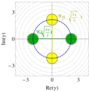
a)       b)

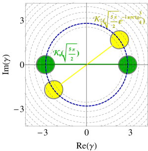
Figure 5: Phase space representation of orthogonal vectors ${\mathcal{K}}_{\scriptscriptstyle{0}}(\alpha)$ (green) and ${\mathcal{K}}_{\varphi_{\!{}_{2}}}(\beta)$ (yellow) with equal mean number of photons $|\alpha|^{2}=|\beta|^{2}=\sqrt{\omega^{2}+(1/2+k)^{2}\pi^{2}}$, calculated for $k=1$ and a) $\omega=0$; b) $\omega=2\pi$. Dashed circles denote the only possible values fulfilling conditions $\langle{\mathcal{K}}_{\varphi_{\!{}_{1}}}(\alpha)|{\mathcal{K}}_{\varphi_{\!{}_{2}}}(\beta)\rangle=0$ and $|\alpha|=|\beta|$, for given $\omega$. Width of the bands between subsequent circles strongly depend on $\omega$: in case a) corresponding to odd cat-like superpositions, described in Section 2.2, areas of subsequent bands are always equal to $\pi^{2}$. In case b) areas of the bands depend on $k$ and are equal to $\pi^{2}$ only in the limit of $|k|\rightarrow\infty$.

 

When real part of $\alpha\beta^{*}$ vanishes

Consider a special case when $\omega\!=\!\mathrm{Re}(\alpha\beta^{*})\!=\!0$. If $\cos[2\,\mathrm{Im}(\alpha\beta^{*})]=1$, from (9a) follows that one of the phases $\varphi_{\!{}_{1}}$, $\varphi_{\!{}_{2}}$ has to be equal to $\pi$, the other can be arbitrary. If $\cos[2\,\mathrm{Im}(\alpha\beta^{*})]=-1$, one of the phases has to be equal to $0$ and the other is arbitrary. In Fig. 4 the former case is denoted by the dashed white lines, the later by dashed blue lines, i.e. edges of a larger yellow-green square. Note, that the case when $(\varphi_{\!{}_{1}},\varphi_{\!{}_{2}})\mathrel{\raisebox{1.0pt}{$\!{\scriptstyle\in}\!$}}\{(0,\pi),(\pi,0)\}$ takes us once again to the orthogonality between odd and even cats. It is clear that in this case, for a known $\alpha\neq 0$ and one and only one of the phases equal to 0 or $\pi$, value of $\beta$ is determined unambiguously, while the second phase is arbitrary.

From now on we will assume that real part of $\alpha\beta^{*}$ is nonzero, which means that we will consider only phases depicted in Fig. 4 by green or yellow open triangles (without edges).

III.2.1 Set values of $\varphi_{\!{}_{1}}$, $\varphi_{\!{}_{2}}$ and $\alpha$

To avoid repetitions, we assume now that $\cos({\scriptstyle{\frac{\varphi_{\!{}_{2}}+\varphi_{\!{}_{1}}}{2}}})\cos({\scriptstyle{\frac{\varphi_{\!{}_{2}}-\varphi_{\!{}_{1}}}{2}}})\neq 0\,$ and that $\varphi_{\!{}_{1}},\varphi_{\!{}_{2}}$ are different then 0 or $\pi$. For given phases $\varphi_{\!{}_{1}}$, $\varphi_{\!{}_{2}}$, quantization condition depends on whether point $(\varphi_{\!{}_{1}},\varphi_{\!{}_{2}})$ belongs to a green or yellow areas in Fig. 4 . In the first case, phases are such that ${\cos(\frac{\varphi_{\!{}_{1}}-\varphi_{\!{}_{2}}}{2})}/{\cos(\frac{\varphi_{\!{}_{1}}+\varphi_{\!{}_{2}}}{2})}<0$, which imposes condition (9a) and, consequently, (9b). The second case, when ${\cos(\frac{\varphi_{\!{}_{1}}-\varphi_{\!{}_{2}}}{2})}/{\cos(\frac{\varphi_{\!{}_{1}}+\varphi_{\!{}_{2}}}{2})}>0$ leads to conditions (10a) and (10b). In both cases, for a known $\varphi_{\!{}_{1}}$, $\varphi_{\!{}_{2}}$ and $\alpha\neq 0$, value of $\beta$ can be determined from (11).

Table 1 summarizes the results obtained so far:

Table 1. Values of $\beta$ such that $\langle{\mathcal{K}}_{\varphi_{\!{}_{2}}}\!(\beta)|{\mathcal{K}}_{\varphi_{\!{}_{1}}}\!(\alpha)\rangle=0$ for given $\alpha,\varphi_{\!{}_{1}}$, $\varphi_{\!{}_{2}}$.
$(\varphi_{\!{}_{1}}$, $\varphi_{\!{}_{2}})\mathrel{\raisebox{1.0pt}{$\!{\scriptstyle\in}\!$}}$ (green surface in Fig. 4)	$\Rightarrow\,\beta_{k}=(\omega-ik\pi)/\alpha^{*},\;\;\;k\mathrel{\raisebox{1.0pt}{$\!{\scriptstyle\in}\!$}}\mathbb{Z}$
$(\varphi_{\!{}_{1}}$, $\varphi_{\!{}_{2}})\mathrel{\raisebox{1.0pt}{$\!{\scriptstyle\in}\!$}}$ (yellow surface in Fig. 4)	$\Rightarrow\,\beta_{k}=(\omega-i(k+1/2)\pi)/\alpha^{*},\;\;k\mathrel{\raisebox{1.0pt}{$\!{\scriptstyle\in}\!$}}\mathbb{Z}$
$(\varphi_{\!{}_{1}}$, $\varphi_{\!{}_{2}})\mathrel{\raisebox{1.0pt}{$\!{\scriptstyle\in}\!$}}$ (red dots in Fig. 4)	$\Rightarrow\,$ arbitrary $\beta$
$(\varphi_{\!{}_{1}}$, $\varphi_{\!{}_{2}})\mathrel{\raisebox{1.0pt}{$\!{\scriptstyle\in}\!$}}$ (black segments in Fig. 4)	$\Rightarrow\,$ no solutions

III.2.2 Set values of $\alpha$, $\beta$ and $\varphi_{\!{}_{1}}$

To analyze conditions (9a), (10a), for set values of $\alpha$, $\beta$ and $\varphi_{\!{}_{1}}$ or set $\alpha$, $\beta$ and $\varphi_{\!{}_{2}}$, it is convenient to introduce new variables: $a=\mathrm{tg}\big{(}\frac{\varphi_{\!{}_{1}}}{4}\big{)}$, $b=\mathrm{tg}\big{(}\frac{\varphi_{\!{}_{2}}}{4}\big{)}$, that transform (9a)-(10a) into analytically solvable quadratic equations. After some calculations it can be shown that, for given $\alpha$, $\beta$ and $\varphi_{\!{}_{1}}$, solutions of (10a) for $\varphi_{\!{}_{2}}$ are

$$\textstyle\varphi_{\!{}_{2}}^{+}=\arctan\!\left[\frac{\sqrt{W(\varphi_{\!{}_{1}},\alpha,\beta)^{2}+U(\varphi_{\!{}_{1}},\alpha,\beta)^{2}}-W(\varphi_{\!{}_{1}},\alpha,\beta)}{U(\varphi_{\!{}_{1}},\alpha,\beta)}\right]\;\mathrm{if}\;\mathrm{Re}(\alpha\beta^{\ast})>0,$$ (13)

$$\textstyle\varphi_{\!{}_{2}}^{-}=\arctan\!\left[\frac{\sqrt{W(\varphi_{\!{}_{1}},\alpha,\beta)^{2}+U(\varphi_{\!{}_{1}},\alpha,\beta)^{2}}+W(\varphi_{\!{}_{1}},\alpha,\beta)}{-U(\varphi_{\!{}_{1}},\alpha,\beta)}\right]\;\mathrm{if}\;\mathrm{Re}(\alpha\beta^{\ast})<0,$$

$$\mathrm{where} W(\varphi_{\!{}_{1}},\alpha,\beta):=2\tan({\textstyle{\frac{\varphi_{\!{}_{1}}}{4}}})\big{[}1+\exp(2\mathrm{Re}(\alpha\beta^{\ast}))\big{]},$$ (14)

$$U(\varphi_{\!{}_{1}},\alpha,\beta):=\big{[}1-\exp(2\mathrm{Re}(\alpha\beta^{\ast}))\big{]}\big{[}(\tan({\textstyle{\frac{\varphi_{\!{}_{1}}}{4}}}))^{2}-1\big{]}.$$

Analogously, after introducing

$$W^{\prime}(\varphi_{\!{}_{1}},\alpha,\beta):=2\tan({\textstyle{\frac{\varphi_{\!{}_{1}}}{4}}})\big{[}1-\exp(2\mathrm{Re}(\alpha\beta^{\ast}))\big{]},$$ (15)

$$U^{\prime}(\varphi_{\!{}_{1}},\alpha,\beta):=\big{[}1+\exp(2\mathrm{Re}(\alpha\beta^{\ast}))\big{]}\big{[}(\tan({\textstyle{\frac{\varphi_{\!{}_{1}}}{4}}}))^{2}-1\big{]},$$

solution of (9a) can be written as

$$\textstyle\varphi_{\!{}_{2}}^{\prime+}=\arctan\!\left[\frac{\sqrt{W^{\prime}(\varphi_{\!{}_{1}},\alpha,\beta)^{2}+U^{\prime}(\varphi_{\!{}_{1}},\alpha,\beta)^{2}}-W^{\prime}(\varphi_{\!{}_{1}},\alpha,\beta)}{U^{\prime}(\varphi_{\!{}_{1}},\alpha,\beta)}\right]\;\mathrm{for}\;\mathrm{Re}(\alpha\beta^{\ast})>0,$$ (16)

$$\textstyle\varphi_{\!{}_{2}}^{\prime-}=\arctan\!\left[\frac{\sqrt{W^{\prime}(\varphi_{\!{}_{1}},\alpha,\beta)^{2}+U^{\prime}(\varphi_{\!{}_{1}},\alpha,\beta)^{2}}+W^{\prime}(\varphi_{\!{}_{1}},\alpha,\beta)}{-U^{\prime}(\varphi_{\!{}_{1}},\alpha,\beta)}\right]\;\mathrm{for}\;\mathrm{Re}(\alpha\beta^{\ast})<0.$$

We have shown unambiguous solutions of (7) in the case of known parameters $\alpha$, $\beta$ and $\varphi_{\!{}_{1}}$. In the case when $\varphi_{\!{}_{1}}$ is a variable and $\varphi_{\!{}_{2}}$ a known parameter, values of $\varphi_{\!{}_{1}}$ can be find in the same fashion because all the equations used were symmetric under transformation $\varphi_{\!{}_{1}}\leftrightarrow\varphi_{\!{}_{2}}$. This ends analysis of equation (7).

To summarize results of this subsection: If $\cos[2\,\mathrm{Im}(\alpha\beta^{\ast})]\!=\!\pm 1$ one can always find phases $\varphi_{\!{}_{1}},\varphi_{\!{}_{2}}$ such that $|{\mathcal{K}}_{\varphi_{\!{}_{2}}}\!(\beta)\rangle$ is orthogonal to $|{\mathcal{K}}_{\varphi_{\!{}_{1}}}\!(\alpha)\rangle$. Moreover,

• for $\mathrm{Re}(\alpha\beta^{\ast})>0$ and any $\varphi_{\!{}_{1}}$ different then 0 or $\pi$ there exists exactly one $\varphi_{\!{}_{2}}$ that makes respective vectors orthogonal. Both $\varphi_{\!{}_{1}}$ and $\varphi_{\!{}_{2}}$ are simultaneously smaller or larger then $\pi$.

• for $\mathrm{Re}(\alpha\beta^{\ast})<0$ and any $\varphi_{\!{}_{1}}$ different then 0 or $\pi$ there exists exactly one $\varphi_{\!{}_{2}}$ that makes respective vectors orthogonal, and either $\varphi_{\!{}_{1}}$ or $\varphi_{\!{}_{2}}$ is larger then $\pi$.

• for $\mathrm{Re}(\alpha\beta^{\ast})=0$ and $\cos[2\,\mathrm{Im}(\alpha\beta^{\ast})]=1$, to obtain orthogonality one phase has to be equal to $\pi$, the other phase can be arbitrary (white dashed lines in Fig. 4). Special case when $(\varphi_{\!{}_{1}},\varphi_{\!{}_{2}})\mathrel{\raisebox{1.0pt}{$\!{\scriptstyle\in}\!$}}\{(0,\pi),(\pi,0)\}$ corresponds to the always orthogonal cat-like superpositions of different parity.

• for $\mathrm{Re}(\alpha\beta^{\ast})=0$ and $\cos[2\,\mathrm{Im}(\alpha\beta^{\ast})]=-1$, one of the phases has to be equal to $0$, second can be arbitrary (dashed blue lines in Fig. 4). Special case, $(\varphi_{\!{}_{1}},\varphi_{\!{}_{2}})\mathrel{\raisebox{1.0pt}{$\!{\scriptstyle\in}\!$}}\{(0,\pi),(\pi,0)\},$ corresponds to the always orthogonal cat-like superpositions of different parity.

IV Summary and outlook

We have presented a full analytical solution of a problem of finding orthogonal vectors within a set of cat-like superpositions of coherent states, (2). We have shown that in the case of known $\alpha,\beta$, and $\varphi_{\!{}_{1}}$ the condition $\langle{\mathcal{K}}_{\varphi_{\!{}_{2}}}(\beta)|{\mathcal{K}}_{\varphi_{\!{}_{1}}}(\alpha)\rangle=0\,$ determines $\varphi_{\!{}_{2}}$ unambiguously, thus, measurements of the scalar product can be used to measure the phase. We have also shown that for any given cat-like superposition ${\mathcal{K}}_{\varphi_{\!{}_{1}}}\!(\alpha)$ and set $\varphi_{\!{}_{2}}$, such that $(\varphi_{\!{}_{1}},\varphi_{\!{}_{2}})$ belongs to either green or yellow areas in Fig. 4, there exist a whole family of vectors of the form ${\mathcal{K}}_{\varphi_{\!{}_{2}}}\!(\beta)$ orthogonal to ${\mathcal{K}}_{\varphi_{\!{}_{1}}}\!(\alpha)$, and have presented an explicit solutions. We have proved that the considered orthogonality condition imposes on antisymmetric (simplectic) form $\mathrm{Im}(\alpha\beta^{*})$ a quantization condition permitting only discreet values, and has no such restriction on metric form $\mathrm{Re}(\alpha\beta^{*})$.

Results presented in this paper show, among others, that structures build from superposition of coherent states let directly deterministically distinguish between them – in contrast to only probabilistic distinguisability between ‘single’ coherent states. This fact has potentially many applications: from ability to perfectly distinguish different cat states follows, in principle, possibility to use precise measurement of a scalar product for a precise measurement of phase, and vice versa. In the context of quantum communication, existence of infinite sets of orthogonal states allows to send binary sequences without repetition of code words, and a condition $\cos[2\,\mathrm{Im}(\alpha\beta^{\ast})]=\pm 1$ adds a possibility of additional spin-like encoding.

Acknowledgments L.P. thanks Prof. Ray-Kuang Lee for his hospitality and stimulating discussions. This work was supported by NTHU project no. 104N1807E1.

Appendix A: Notation

In this paper a standard notation was used: Greek letters $\alpha,\beta,\gamma...$ denote complex numbers and $|\alpha\rangle,|\beta\rangle,|\gamma\rangle$ are the corresponding coherent states. Set of real and complex numbers are denoted by $\mathbb{R}$ and $\mathbb{C}$, respectively, while $\mathbb{R}^{\times}$ and $\mathbb{C}^{\times}$ denote sets of real or complex numbers without zero. A set of integer numbers is denoted as $\mathbb{Z}$, and a set of natural numbers (with zero) as $\mathbb{N}$, whereas $\mathbb{N}^{\times}\mathrel{\mathop{:}}=\mathbb{N}\mathrel{\raisebox{1.0pt}{$\!{\scriptstyle\setminus}\!$}}\{0\}$.

Appendix B:

Decomposition of a complex number $\gamma\mathrel{\raisebox{1.0pt}{$\!{\scriptstyle\in}\!$}}\mathbb{C}$ into real and imaginary parts, $\mathrm{Re}(\gamma)$ and $\mathrm{Im}(\gamma)$, defines a canonical isomorphism of real vector spaces

$$\vec{{}}\,:\mathbb{C}\mathrel{\raisebox{1.0pt}{$\!{\scriptstyle\ni}\!$}}\gamma\rightarrow\vec{\gamma}\mathrel{\mathop{:}}=\left(\!\!\!\begin{array}[]{c}\mathrm{Re}(\gamma)\\ \mathrm{Im}(\gamma)\end{array}\!\!\!\right)\mathrel{\raisebox{1.5pt}{$\!{\scriptstyle\in}\!$}}\mathbb{R}^{2}.$$ (19)

It means that the multiplication of complex numbers $\alpha\beta^{*}$ defines two bilinear forms on $\mathbb{R}^{2}$

$$g:\mathbb{R}^{2}\!\mathrel{\raisebox{1.0pt}{$\!{\scriptstyle\times}\!$}}\mathbb{R}^{2}\mathrel{\raisebox{1.0pt}{$\!{\scriptstyle\ni}\!$}}(\vec{\alpha},\vec{\beta})\rightarrow g(\vec{\alpha},\vec{\beta})\mathrel{\mathop{:}}=\mathrm{Re}(\alpha\beta^{*})\mathrel{\raisebox{1.0pt}{$\!{\scriptstyle\in}\!$}}\mathbb{R}$$ (20)

$$h:\mathbb{R}^{2}\!\mathrel{\raisebox{1.0pt}{$\!{\scriptstyle\times}\!$}}\mathbb{R}^{2}\mathrel{\raisebox{1.0pt}{$\!{\scriptstyle\ni}\!$}}(\vec{\alpha},\vec{\beta})\rightarrow h(\vec{\alpha},\vec{\beta})\mathrel{\mathop{:}}=\mathrm{Im}(\alpha\beta^{*})\mathrel{\raisebox{1.0pt}{$\!{\scriptstyle\in}\!$}}\mathbb{R}.$$ (21)

Form $g$ is symmetric and defines a metric (Riemann) structure on $\mathbb{R}^{2}$. Form $h$ is antisymmetric and defines a symplectic structure on $\mathbb{R}^{2}$.

Results of Section 3.2 show that orthogonality condition between vectors ${\mathcal{K}}_{\varphi_{\!{}_{1}}}\!(\alpha)$ and ${\mathcal{K}}_{\varphi_{\!{}_{2}}}\!(\beta)$ impose quantization condition on possible values of symplectic form $h(\vec{\alpha},\vec{\beta})$ on $\mathbb{R}^{2}$, as it is clearly seen from (9b) and (10b). At the same time connected with phases $\varphi_{\!{}_{1}},\varphi_{\!{}_{2}}$ values of metric form $g(\vec{\alpha},\vec{\beta})$ can take on arbitrary real values and are continuous (see (9a) and (10a)).

References

- (1) E. Schrödinger, Der stetige übergang von der mikro- zur makromechanik, Naturwissenschaften 14 (1926) 664.
- (2) J. von Neumann, Mathematische Grundlagen der Quantenmechanik,, Springer, Berlin, 1932.
- (3) R. Glauber, The quantum theory of optical coherence, Phys. Rev. 130 (1963) 2529.
- (4) P. T. Cochrane, G. J. Milburn, W. J. Munro, Macroscopically distinct quantum-superposition states as a bosonic code for amplitude damping, Phys. Rev. A 59 (1999) 2631.
- (5) S. J. van Enk, O. Hirota, Entangled coherent states: Teleportation and decoherence, Phys. Rev. A 64 (2001) 022313.
- (6) H. Jeong, M. S. Kim, Efficient quantum computation using coherent states, Phys. Rev. A 65 (2002) 042305.
- (7) T. C. Ralph, A. Gilchrist, G. J. Milburn, W. J. Munro, S. Glancy, Quantum computation with optical coherent states, Phys. Rev. A 68 (2003) 042319.
- (8) A. Ourjoumtsev, R. Tualle-Brouri, J. Laurat, P. Grangier, Generating optical schrödinger kittens for quantum information processing, Science 312 (2006) 83.
- (9) A. Ourjoumtsev, H. Jeong, R. Tualle-Brouri, P. Grangier, Generation of optical schrödinger cats from photon number states, Nature 448 (2007) 06054.
- (10) H. Takahashi, K. Wakui, S. Suzuki, M. Takeoka, K. Hayasaka, A. Furusawa, M. Sasaki, Generation of large-amplitude coherent-state superposition via ancilla-assisted photon-subtraction, Phys. Rev. Lett. 101 (2008) 233605.
- (11) E. Schrödinger, Die gegenwartige situation in der quantenmechanik, Naturwissenschaften 23 (1935) 807.
- (12) M. Hillery, Amplitude-squared squeezing of the electromagnetic field, Phys. Rev. A 36 (1987) 3796.
- (13) W. Schleich, M. Pernigo, F. L. Kien, Nonclassical state from two pseudoclassical states, Phys. Rev. A 44 (1991) 2172.
- (14) E. Wigner, On the quantum correction for thermodynamic equilibrium, Phys. Rev. 40 (1932) 749.
- (15) V. Buzek, P. Knight, Quantum interference, superposition states of light, and nonclassical effects, in: Prog. in Opt. XXXIV, Elsevier Ltd., 1995.
- (16) W. H. Zurek, Decoherence and the transition from quantum to classical – revisited, arXiv:quant-ph/0306072v1.
- (17) A. Perelomov, Generelized Coherent States and Their Applications, Springer-Verlag, Berlin Heidelberg, 1986.
- (18) J.-P. Gazeau, Coherent States in Quantum Physics, WILEY-VCH Verlag, Weincheim, 2009.
- (19) L. Praxmeyer, P. Wasylczyk, C. Radzewicz, K. Wódkiewicz, Time-frequency domain analogues of phase space sub-planck structures, Phys. Rev. Lett. 98 (2007) 063901.
- (20) K. Husimi, Some formal properties of the density matrix, Proc. Phys. Math. Soc. Jpn. 22 (1940) 264.