Recursive dynamic mode decomposition of a transient cylinder wake

Abstract

A novel data-driven modal decomposition of fluid flow is proposed comprising key features of POD and DMD. The first mode is the normalized real or imaginary part of the DMD mode which minimizes the time-averaged residual. The $N$-th mode is defined recursively in an analogous manner based on the residual of an expansion using the first $N-1$ modes. The resulting recursive DMD (RDMD) modes are orthogonal by construction, retain pure frequency content and aim at low residual. RDMD is applied to transient cylinder wake data and is benchmarked against POD and optimized DMD (Chen et al., 2012) for the same snapshot sequence. Unlike POD modes, RDMD structures are shown to have pure frequency content while retaining a residual of comparable order as POD. In contrast to DMD with exponentially growing or decaying oscillatory amplitudes, RDMD clearly identifies initial, maximum and final fluctuation levels. Intriguingly, RDMD outperforms both POD and DMD in the limit cycle resolution from the same snaphots. RDMD is proposed as an attractive alternative to POD and DMD for empirical Galerkin models, with nonlinear transient dynamics as a niche application.

1 Introduction

This study proposes a novel flow field expansion tailored to the construction of low-dimensional empirical Galerkin models. Such reduced-order models (1) help in data compression, (2) allow quick visualizations and kinematic mixing studies (Rom-Kedar et al., 1990), (3) provide a testbed for physical understanding (Lorenz, 1963), (4) serve as computationally inexpensive surrogate models for optimization (Han et al., 2013) or (5) may be used as a plant for control design (Gerhard et al., 2003; Bergmann & Cordier, 2008).

In 1858, Helmholtz has laid the foundation for the first low-dimensional dynamical models in fluid mechanics with his famous theorems on vortices (see, e.g. Lugt, 1995). Subsequently, a rich set of vortex models have been developed for vortex pairs, for the recirculation zone (Föppl, 1913; Suh, 1993), for the vortex street (von Kármán & Rubach, 1912), and for numerous combustion related problems (Coats, 1997), to name just a few. For non-periodic open flows, low-dimensional vortex models come at the expense of a hybrid state-space structure: new degrees of freedom (vortices) are created at the body, merged or removed. Most forms of applications, like dynamical systems analyses or control design, are not suitable for hybrid models but assume a continuous evolution in a fixed finite-dimensional state space. Hence, most currently developed reduced-order models are formulated by the Galerkin method and based on modal expansions (Fletcher, 1984).

In the last 100 years Galerkin (1915)’s method of solving partial differential equations has enjoyed ample generalisations and applications, from high-dimensional grid-based computational methods to low-dimensional models. This study focusses on low-dimensional flow representations by an expansion in global modal structures. In principle, any space of square-integrable velocity fields has a complete set of orthonormal modes: any flow field can be arbitrarily closely approximated by a finite-dimensional expansion. In practice, however, the construction of such mathematical bases is restricted to simple geometries and the use of Fourier expansions or Chebyshev polynomials (Orszag, 1971). Stability modes based on a linearisation of the Navier-Stokes equation tend to be more efficient in terms of resolution for a given number $N$ of modes. However, these physical modes generally lack a proof of completeness, and are afflicted by a reduced dynamic bandwidth and an ${\cal{O}}(N^{3})$ operation count for the quadratic terms as opposed to ${\cal{O}}(N\log N)$ operations for Fourier or Chebyshev modes. The most efficient representations of a Navier-Stokes solution are obtained from empirical expansions based on flow snapshots. These data-driven Galerkin expansions are confined to a subspace spanned by the snapshots, i.e. have a narrow dynamic bandwidth defined by the training set.

This study focusses on data-driven expansions. A Galerkin expansion with guaranteed minimal residual over the training snapshots was first pioneered by Lorenz (1956) as principal axis modes and later popularized in fluid mechanics as proper orthogonal decomposition (POD) by Lumley (1967). POD guarantees an optimal data reconstruction in a well-defined sense (see, e.g., Holmes et al., 1998). Apart from data compression applications, Lumley devised POD as a mathematical tool for distilling coherent structures from data. Yet, only in rare cases have POD modes been found to resemble physically meaningful structures, like stability modes or base-flow deformations (Oberleithner et al., 2011). In particular, they tend to mix spatial and temporal frequencies in most modes which complicates a physical interpretation. As a remedy for this shortcoming, the dynamic mode decomposition (DMD) — also referred to as Koopman analysis — was pioneered by Rowley et al. (2009) and Schmid (2010). DMD is able to distill stability eigenmodes from transient snapshot data and produce temporal Fourier modes for post-transient data. The downside of these DMD features — as compared to POD — are non-orthogonality of the extracted modes, suboptimal convergence, the need for time-resolved snapshots and numerical challenges when filtering is omitted. Over the past, numerous Galerkin models based on POD and DMD have been constructed. In addition, numerous generalisations have been proposed to address, among other topics, multi-operating conditions (Jørgensen et al., 2003), changes during transients (Siegel et al., 2008), optimal correlations to observables (Hoarau et al., 2006; Schlegel et al., 2012), and control design (Brunton & Noack, 2015).

This study proposes a novel data-driven expansion preserving key features of POD, such as orthonormality of the computed modes and a low residual, and of DMD, such as distilling the dominant frequencies and their associated structures contained in the data. The manuscript is organised as follows. § 2 describes the cylinder wake configuration and gives details on the employed direct numerical simulation as well as the extracted snapshots. § 3 outlines the computation of the proposed expansion, called ’Recursive DMD (RDMD)’ in what follows. RDMD is then applied to a transient cylinder wake, demonstrating its advantages (§ 4) over previous decompositions. Our results are summarised in § 5.

2 Configuration and direct numerical simulation

As a test-case, a two-dimensional, incompressible, viscous flow past a circular cylinder has been chosen. The flow is described in a Cartesian coordinate system where the $x$-axis is aligned with streamwise direction and the $y$-axis is transverse and orthogonal to the cylinder axis. The origin of the coordinate system coincides with the cylinder axis. The location vector is denoted by $\bm{x}=(x,y)$. Analogously, the velocity is represented by $\bm{u}=(u,v)$ where $u$ and $v$ are the $x$- and $y$-components of the velocity components. The time is presented by $t$. The Newtonian fluid is characterised by the density $\rho$ and dynamic viscosity $\mu$. In the following, all variables are assumed to be nondimensionalised by the cylinder’s diameter $D$, the oncoming velocity $U$ and the fluid density $\rho$. The resulting Reynolds number $Re=UD\rho/\mu$ is set to $100$, i.e. well above the onset of vortex shedding (Zebib, 1987; Schumm et al., 1994), but well below the onset of three-dimensional instabilities (Zhang et al., 1995; Barkley & Henderson, 1996; Williamson, 1996).

A direct numerical simulation of the Navier-Stokes equations has been performed using an in-house solver based on a second-order finite-element discretisation with Taylor-Hood elements (Taylor & Hood, 1973) in penalty formulation. The time stepping is performed using a third-order accurate scheme and a time step equal to $0.1$. Following Noack et al. (2003), the computational domain extends from $x=-5$ to $x=25$ and $y=-5$ to $y=5$ and is discretised with 56272 finite elements.

The simulation provides $M=450$ equidistantly sampled velocity snapshots $\bm{u}^{m}(\bm{x})=\bm{u}(\bm{x},t^{m})$, $m=1,..,M$, covering the entire unforced transient phase, from the steady solution to the fully-developed von Kármán vortex street. The snapshot times are $t^{m}=30+m\Delta t$ based on a sampling interval $\Delta t=0.2$ and cover the time interval $t\in[30,120].$ The initial and final base flows are depicted in figure 1 together with the energy norm of the fluctuations $\bm{v}=\bm{u}-\bm{u}_{s}$ around the steady solution $\bm{u}_{s}$. The transition from the unstable fixed point to the stable limit-cycle oscillation is characterised by the growing amplitudes of the fluctuations accompanied by an increase in the Strouhal number (Zebib, 1987; Schumm et al., 1994).

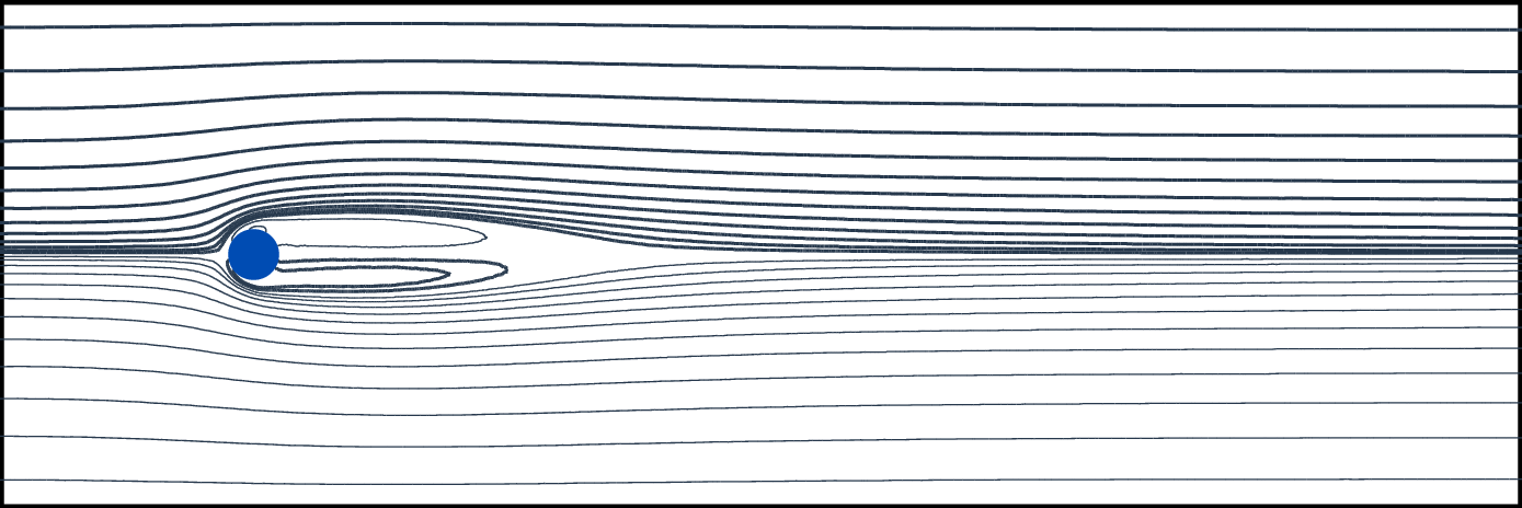
Figure 1: Incompressible two-dimensional flow around a circular cylinder at $Re=100$. The steady (top-left) and time-averaged (top-right) solutions are illustrated with streamlines. The total fluctuation level normalized with its asymptotic value is monitored below.

Within the first 30 convective time units, the flow is governed by linear dynamics spanned by the steady solution and the unstable eigenmode. In the intermediate phase, approximately $t\in[60,90]$, the vortex shedding undergoes significant chances and moves farther upstream towards the cylinder. In the final 30 convective time units, the flow has converged to a limit-cycle dynamics exhibiting the fully-developed von Kármán vortex street. These three characteristic stages of the transient evolution are depicted in figure 2.

Figure 2: Transient evolution of the cylinder wake illustrated with snapshots of the vorticity field at an initial (left, $t=50$), an intermediate (middle, $t=70$) and final state (right, $t=90$).

All modal decompositions are based on these fluctuations around the steady solution. The mean flow is discarded as a base flow because it is only well defined for this particular initial condition and the chosen time interval. Our sampling Strouahl frequency of $10$ is about 30 times larger than the shedding frequency – a value which can be considered adequate for a Fourier transformation while avoiding excessive redundancy for the statistical POD.

3 Modal decomposition

In this section, a new snapshot-based modal decomposition is proposed. This decomposition comprises properties of the Proper Orthogonal Decomposition (POD) (Lumley, 1967; Sirovich, 1987) and the Dynamic Mode Decomposition (DMD) (Rowley et al., 2009; Schmid, 2010). First (§ 3.1 & 3.2), the snapshot-based POD and DMD are briefly recapitulated. In § 3.3, the recursive DMD (RDMD) is proposed as an appealing compromise inheriting the orthonormality and low truncation error of POD and the oscillatory representation of the flow behaviour of DMD.

3.1 Proper Orthogonal Decomposition

We analyse a time-dependent velocity field $\bm{u}(\bm{x},t)$ in a steady domain $\bm{x}\in\Omega$ and sample $M$ flow snapshots with constant sampling frequency corresponding to a time step $\Delta t$. The velocity field at instant $t^{m}=m\Delta t$, with $m=1,\ldots,M,$ is denoted by $\bm{u}^{m}:=\bm{u}(\bm{x},t^{m})$.

POD requires the definition of an inner product and a time average. We assume the standard inner product of two square-integrable velocity fields $\bm{u}$, $\bm{v}\in{\cal L}^{2}(\Omega),$ given as

$$\left(\bm{u},\bm{v}\right)_{\Omega}:=\int\limits_{\Omega}d\bm{x}\>\bm{u}(\bm{x})\cdot\bm{v}(\bm{x}).$$ (1)

The corresponding norm reads $\|\bm{u}\|_{\Omega}:=\sqrt{\left(\bm{u},\bm{u}\right)_{\Omega}}$. The snapshot-based time average of a function $F$ is defined in a canonical manner:

$$\langle F(\bm{u})\rangle_{M}:=\frac{1}{M}\sum\limits_{m=1}^{M}F\left(\bm{u}^{m}\right).$$ (2)

In the following, the snapshot-based POD (Sirovich, 1987) is applied to the fluctations $\bm{v}^{m}(\bm{x}):=\bm{v}(\bm{x},t^{m})-\bm{u}_{s}(\bm{x})$ around the steady solution $\bm{u}_{s}$ for the reasons mentioned in § 2. First, the correlation matrix $\bm{C}=\left(C^{mn}\right)\in{\Bbb{R}}^{M\times M}$ of the fluctuations is determined,

$$C^{mn}:=\frac{1}{M}\left(\bm{v}^{m},\bm{v}^{n}\right)_{\Omega}.$$ (3)

Second, a spectral analysis of this matrix is performed. Note that $\bm{C}$ is a symmetric, positive semi-definite Gramian matrix. Hence, its eigenvalues $\lambda_{i}$ are real and nonnegative and can be assumed to be sorted according to $\lambda_{1}\geq\lambda_{2}\geq\ldots\geq\lambda_{M}\geq 0$. The corresponding eigenvectors $\bm{e}_{i}=\left[e_{i}^{1},\ldots,e_{i}^{M}\right]^{T}$ satisfy

$$\bm{C}\bm{e}_{i}=\lambda_{i}\bm{e}_{i},\qquad i=1,\ldots,M.$$ (4)

and can – without loss of generality – be assumed to be orthonormalized, satisfying $\bm{e}_{i}\cdot\bm{e}_{j}=\delta_{ij}$ with $\delta_{ij}$ as the Kronecker symbol. Third, each POD mode is expressed as a linear combination of the snapshot fluctuations,

$$\bm{u}_{i}:=\frac{1}{\sqrt{M\>\lambda_{i}}}\>\sum\limits_{m=1}^{M}e_{i}^{m}\>\bm{v}^{m},\qquad i=1,\ldots,N.$$ (5)

It follows that the POD modes are orthonormal, with $\left(\bm{u}_{i},\bm{u}_{j}\right)_{\Omega}=\delta_{ij},\quad\forall i,j\in\{1,\ldots,M\}$. Finally, the mode amplitudes read

$$a_{i}^{m}:=\sqrt{\lambda_{i}\>M}\>e^{i}_{m},\qquad i=1,\ldots,N.$$ (6)

These amplitudes are uncorrelated (orthogonal in time), or in mathematical terms

$$\langle a_{i}a_{j}\rangle_{M}=\lambda_{i}\>\delta_{ij},\qquad i,j\in\{1,\ldots,N\}.$$ (7)

Note that the first moments $\langle a_{i}\rangle_{M}$ do not need to vanish as the fluctuations are based on the steady solution and not on the mean flow of this transient. The POD defines a second-order statistics providing the two-point autocorrelation function

$$\overline{\bm{v}(\bm{x},t)\>\bm{v}(\bm{y},t)}=\sum\limits_{i=1}^{N}\lambda_{i}\>\bm{u}_{i}(\bm{x})\>\bm{u}_{i}(\bm{y}).$$ (8)

Hence, a minimum requirement imposed on the snapshot ensemble is the accuracy of the extracted mean flow and the flow’s second moments. This accuracy of the statistics for a given number of snapshots is increased by processing uncorrelated snapshots as required in the original paper on the snapshot POD method (Sirovich, 1987).

The resulting expansion exactly reproduces the snapshots for $N=M$ modes; we have

$$\bm{u}(\bm{x},t^{m})=\bm{u}_{s}(\bm{x})+\sum\limits_{i=1}^{N}a_{i}(t^{m})\>\bm{u}_{i}(\bm{x}).$$ (9)

For $N<M$, the truncated expansion (9) has a non-vanishing residual $\bm{r}^{m}(\bm{x}):=\bm{r}(\bm{x},t^{m})$. The corresponding time-averaged truncation error

$$\chi^{2}:=\langle\|\bm{r}^{m}\|_{\Omega}^{2}\rangle_{M}$$ (10)

can be shown to be minimal; in other words, no other Galerkin expansion will have a smaller error (Holmes et al., 1998). This optimality property makes POD an attractive data compression technique.

For later reference, the instantaneous truncation error $\chi^{2}(t):=\|\bm{r}^{m}(\cdot,t)\|_{\Omega}^{2}$ is introduced. The size of this error may be compared with the corresponding fluctuation level on the limit cycle $2K_{\infty}=\overline{\|\bm{v}\|^{2}}$, were $K_{\infty}$ denotes the turbulent kinetic energy (TKE) and the overbar represents averaging over the post-transient phase. We also introduce $K$ as the corresponding instantaneous quantity.

As a motivation for the proposed new decomposition, we recall that POD can also be defined in a recursive manner, following Courant & Hilbert (1989) on the spectral analysis of positive definite symmetric matrices. Taking $\bm{u}_{1}$ as the first expansion mode, the resulting one-mode expansion reads

$$\bm{v}^{m}=a_{1}^{m}\bm{u}_{1}+\bm{r}_{1}^{m},\quad m=1,\ldots,M.$$ (11)

The mode amplitude $a_{1}^{m}:=(\bm{v}^{m},\bm{u}_{1})_{\Omega}$ minimizes the residual $\|\bm{r}_{1}^{m}\|_{\Omega}$ for a given $\bm{u}_{1}$. The first POD mode can be shown to minimize the averaged energy of the residual $\langle\|\bm{r}_{1}^{m}\|_{\Omega}^{2}\rangle_{M}$. Furthermore, the residual $\bm{r}_{1}^{m}$, $m=1,\ldots,M$ is orthogonal to $\bm{u}_{1}$ by construction. The second step then searches for a mode $\bm{u}_{2}$ which best resolves the residual $\bm{r}_{1}$,

$$\bm{r}^{m}_{1}=a_{2}^{m}\bm{u}_{2}+\bm{r}_{2}^{m}\quad m=1,\ldots,M,$$ (12)

i.e. which minimizes $\left\langle\|\bm{r}_{2}^{m}\|_{\Omega}^{2}\right\rangle_{M}$. The other remaining modes are computed in a similar manner.

3.2 Dynamic Mode Decomposition

The Dynamic Mode Decomposition (Rowley et al., 2009; Schmid, 2010) is another data-driven modal expansion which can approximate stability eigenmodes from transient data or Fourier modes from post-transient data. The time step $\Delta t$ needs to be sufficiently small for a meaningful Fourier analysis, but sufficiently large so that the changes in the flow state exceed the noise level.

We consider the fluctuation snaphots of § 3.1, $\bm{v}^{m}$, $m=1,\ldots,M$ as linearly independent modes of an expansion and write

$$\bm{v}=\sum\limits_{i=1}^{M}b_{i}\bm{v}^{i}.$$ (13)

Evidently, the modes are generally not orthogonal. With this basis, the mode amplitude vector of the $m$-th snapshot becomes a unit vector:

$$\bm{b}^{m}=\left[b_{1}^{m},\ldots,b_{M}^{m}\right]^{T}\quad\hbox{where}\quad b_{i}^{m}=\delta_{im}.$$ (14)

DMD assumes a linear relationship between the $(m+1)$-th and $m$-th snapshot

$$\bm{b}^{m+1}=\bm{A}\>\bm{b}^{m},$$ (15)

where $\bm{A}\in{\Bbb{R}}^{M\times M}$ is a square matrix which is generally identified from the data. From Eqn. (15), the matrix is easily seen to be

$$\bm{A}=\left[\begin{array}[]{cccccc}0&0&\ldots&0&0&c_{1}\\ 1&0&\ldots&0&0&c_{2}\\ \vdots&\vdots&\ddots&\vdots&\vdots\\ 0&0&\ldots&1&0&c_{M-1}\\ 0&0&\ldots&0&1&0\end{array}\right].$$ (16)

For $i<M$ the matrix acts as a shift map for the only non-vanishing element of $\bm{b}$. The last snaphot is expanded in terms of the previous ones:

$$\bm{v}^{M}=\sum\limits_{i=1}^{M-1}c_{i}\>\bm{v}^{i}+\bm{r}.$$ (17)

The coefficients $c_{i}$ are chosen to minimize the residual norm $\|\bm{r}\|_{\Omega}$.

In what follows, we depart from the classical DMD literature and propose a simpler derivation of the DMD modes. Let $P(s)=-c_{1}-c_{2}s-\ldots-c_{M-1}s^{M-2}-s^{M}$ be a polynomial in $s$ and let $P(s)=(s-\lambda_{1})(s-\lambda_{2})\ldots(s-\lambda_{M})$ be its factorization with distinct eigenvalues $\lambda_{i}$. We introduce

$$\bm{V}=\left[\begin{array}[]{cccc}1&\lambda_{1}&\ldots&\lambda_{1}^{M-1}\\ 1&\lambda_{2}&\ldots&\lambda_{2}^{M-1}\\ \vdots&\vdots&\vdots&\vdots\\ 1&\lambda_{M}&\ldots&\lambda_{M}^{M-1}\end{array}\right].$$ (18)

as the corresponding Vandermonde matrix. It can be easily verified that the Vandermonde matrix $\bm{V}$ diagonalizes the companion matrix $\bm{A}.$ We obtain

$$\bm{V}\bm{A}\bm{V}^{1}=\hbox{diag}(\lambda_{1},\ldots,\lambda_{M}),$$ (19)

where the right-hand side is a diagonal matrix with the eigenvalues as its elements. We introduce new variables $\bm{a}$ defined by

$$\bm{a}=\bm{V}\bm{b}.$$ (20)

With these definitions, the evolution equation (15) can be cast into eigenform according to

$$\bm{a}^{m+1}=\bm{V}\bm{C}\bm{V}^{-1}\bm{a}^{m}=\bf{D}\bm{a}^{m}.$$ (21)

Here, $\bm{D}$ denotes the diagonal matrix

$$\bm{D}=\hbox{diag}(\lambda_{1},\ldots,\lambda_{M})=\left[\begin{array}[]{cccc}\lambda_{1}&0&\ldots&0\\ 0&\lambda_{2}&\ldots&0\\ \vdots&\vdots&\vdots&\vdots\\ 0&0&\ldots&\lambda_{M}\end{array}\right]$$ (22)

where the $i$-th eigenvalue is $\lambda_{i}$ with corresponding eigenvector $\bm{a}_{i}=\left[\delta_{1i},\ldots,\delta_{Mi}\right]^{T}.$

Equations (14), (15) and (20) imply that the snapshots can be expressed as

$$\bm{v}^{m}=\sum\limits_{i=1}^{M-1}\lambda_{i}^{m-1}\bm{\Phi}_{i}$$ (23)

where $\lambda_{i}$ are referred to as DMD eigenvalues and $\bm{\Phi}_{i}$ as (complex) DMD modes. Note that the derivation of (23) rests on the diagonalization of the companion matrix (19) and does not require the Koopman operator.

The choice of $N$ DMD modes for the Galerkin expansion (9) minimizes the truncation error (10) following Chen et al. (2012) and consistent with the optimal property of POD.

3.3 Recursive Dynamic Mode Decomposition

The recursive Dynamic Mode Decomposition (RDMD) serves a multi-objective task: extracting oscillatory modes from the snapshot sequence (like DMD) while ensuring orthogonality of the modes and a low truncation error (like POD).

The initialisation step prepares the residual to be processed. We take

$$\bm{r}_{0}^{m}:=\bm{v}^{m},\qquad m=1,\ldots,M.$$ (24)

During the $i$-th step ($0<i\leq N$), the $i$-th mode is determined from a DMD

$$\bm{r}_{i-1}^{m}=\sum\limits_{j=1}^{M-1}\lambda_{j}^{m}\>\bm{\Phi}_{j}.$$ (25)

The candidate modes to be considered are

$$\bm{u}_{n}^{\star}=\frac{\Re\{\bm{\Phi}_{n}\}}{\left\|\Re\{\bm{\Phi}_{n}\}\right\|_{\Omega}},$$ (26)

and each mode reduces the snapshot-dependent residual to $\bm{r}_{i}^{m}$ according to

$$\bm{r}_{i-1}^{m} = a_{n}^{m}\bm{u}_{n}^{\star}+\bm{r}_{i}^{m},$$ (27a)

$$a_{n}^{m} = \left(\bm{r}_{i-1}^{m},\bm{u}_{n}^{\star}\right)_{\Omega}.$$ (27b)

The truncation error of the $i$-th candidate mode $\bm{u}_{n}^{\star}$ for all snapshots is given by

$$\chi_{n}^{2}:=\left\langle\left\|\bm{r}_{i}^{m}\right\|^{2}_{\Omega}\right\rangle_{M}.$$ (28)

We then select the mode $i$ with the lowest averaged error, i.e.,

$$\bm{u}_{i}:=\bm{u}_{n}^{\star}\quad\hbox{s.t.}\qquad\forall l\in\{1,\ldots,M\}\colon\chi_{n}^{2}\leq\chi_{l}^{2},$$ (29)

and the resulting expansion, after the $i$-th step, reads

$$\bm{v}_{r}:=\sum\limits_{j=1}^{i}a_{j}\bm{u}_{j}+\rm{r}_{i}^{m}.$$ (30)

The $(i+1)$-th mode is computed following the same steps. The iteration terminates when the desired number of modes is reached, $i=N$, or in the unlikely case that all residuals vanish $\bm{r}_{i}^{m}\equiv 0,\quad m=1,\ldots,M$ — whichever criterion is satisfied first.

4 Modal decomposition of the transient cylinder wake

The transient cylinder wake is analysed with POD (§ 4.1), DMD (§ 4.2) and the proposed new decomposition (§ 4.3) discussed in § 3. In § 4.4 all modal decompositions are subjected to a comparison with respect to the instantaneous residual, the averaged residual and the convergence with increasing number of modes. The transient wake snapshots are the same for all decompositions and have been described in § 2.

4.1 Proper Orthogonal Decomposition (POD)

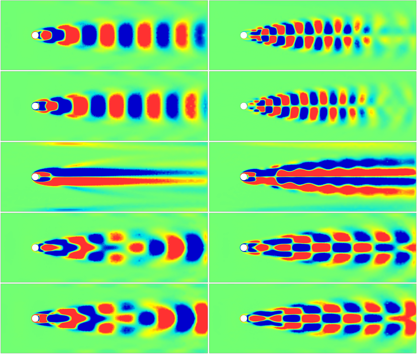
Figure 3: The first ten POD modes of the flow’s transient phase with $t\in[30,120]$ and $Re=100$. The first column contains the modes $1$–$5$ (top to bottom) and the second column modes $6$–$10$ (top to bottom). The vorticity of the mode is visualized in color (green: zero, red: above a positive threshold, blue: below a negative threshold).

The snapshots of the cylinder wake simulations described in § 2 are subjected to a snapshot Proper Orthogonal Decomposition (POD) outlined in § 3.1. The POD modes of the post-transient periodic cylinder wake mimic a Fourier decomposition. They arise in pairs representing the two phases at the first and higher harmonic frequencies (Deane et al., 1991; Noack et al., 2003). The energy level of each pair rapidly decreases with the order of the harmonics. The transient, however, exhibits a gradual change from the initial stability modes (with a fluctuation maximum far from the cylinder) to von Kármán vortex shedding (with fluctuations peaking near the cylinder). The other change is a base flow with a recirculation region which decreases in streamwise extent from about $7$ diameters to about $1$ diameter length. The resulting POD modes and associated mode amplitudes are depicted in figures 3 and 4 and appear different from the post-transient analogs. POD modes 1 and 2 effectively represent von Kármán vortex shedding growing from zero to asymptotic values. These values are larger than the corresponding fluctuation levels of the other modes. Modes 6 and 7 describe the second harmonics as can be seen from the visualisation and the amplitude evolution. Modes 9 and 10 look similar to the stability eigenmodes at slightly lower frequencies with have a peak activity around $t=55.$ Modes 4 and 5 also represent vortex shedding with a peak activity around $t=65$, i.e. two shedding periods later. Mode 3 depicts the shift mode (Noack et al., 2003), i.e. it characterises the base flow change between steady and time-averaged periodic solution. Mode 7 represents another base flow correction with different topology and is mainly active during the most rapid changes of the transient around $t=65$. It has a small second harmonic component.

Figure 4: The mode amplitudes of the POD modes of figure 3 for the corresponding column and row.

All displayed POD modes show pronounced frequencies: six modes display oscillations near the shedding frequency, two resolve the second harmonics and two feature slowly varying base-flow changes. Unlike POD for periodic shedding, there are no traces of the third and higher harmonics in the first $10$ modes. This comparatively ’clean’ frequency content may be attributed to the narrow-bandwidth transient dynamics, with dominant frequencies between the eigenfrequency of the steady solution and the shedding frequency of the post-transient wake. Moreover, the maximum of the fluctuation envelope moves upstream during the transient. For broadband dynamics, such as a mixing layer with multiple vortex pairings, POD modes with multiple frequency content are far more common (Noack et al., 2004).

4.2 Dynamic Mode Decomposition (DMD)

The snapshots of the transient flow have been decomposed with the Dynamic Mode Decomposition. The DMD procedure can identify eigenmodes for the transient data and the Fourier modes for the attractor.

Figure 5: Same as figure 3 but for the first ten DMD modes.

Figure 6: Same as figure 4 but for the first ten DMD modes.

The result of the procedure is a set of complex Ritz vectors and complex eigenvalues characterizing the growth rate and the frequency of the respective mode. The first ten eigenmodes are depicted in figure 5. The first DMD mode corresponds to a real eigenvalue leading to a real Ritz vector. The remaining modes represent the real and imaginary parts of complex Ritz vectors. The phase-shifted analog of the oscillatory mode 10 is mode 11 (not displayed). In figure 6 the corresponding amplitudes of the real modes are displayed.

Modes 1, 6 and 7 act as shift modes and resolve slow base-flow changes. This interpretation is corroborated by the behaviour of the mode amplitudes. The remaining modes describe vortex shedding ($i=2,3,4,5,10$) or its second harmonics ($i=8,9$). The oscillatory mode amplitudes are slowly growing, like the first vortex shedding pair (for $i=2,3$) and the second harmonics (for $i=8,9$), or slowly decaying (for $i=4,5,10$). Intriguingly, the DMD modes describing vortex shedding have nearly identical frequencies and nearly identical shapes. This implies a redundancy which constitutes a challenge for reduced-order modeling.

By construction, the mode amplitudes have an exponentially growing or decaying envelope and can thus give no indication of initial or asymptotic values or temporal periods of maximum activity. In particular, an extrapolation beyond the sampling interval $t\in[30,120]$ is not meaningful. An additional potential challenge for reduced-order modeling is posed by the non-orthogonality of the DMD modes.

Already in the early literature (Rowley et al., 2009; Schmid, 2010; Chen et al., 2012), DMD has been shown to accurately capture the onset of fluctuations in the linear regime or the post-transient behaviour on the attractor. The current results indicate difficulties of the DMD concerning the modal interpretation for a complete transient from the steady solution to the post-transient attractor. This issue has also been pointed out and analyzed by Bagheri (2013). In the next section, we present an alternative DMD decomposition that addresses and removes the above-mentioned challenges.

4.3 Recursive Dynamic Mode Decomposition (RDMD)

In this section, the results of RDMD are presented. The procedure is demonstrated for the same set of snapshots as employed previously for POD and DMD.

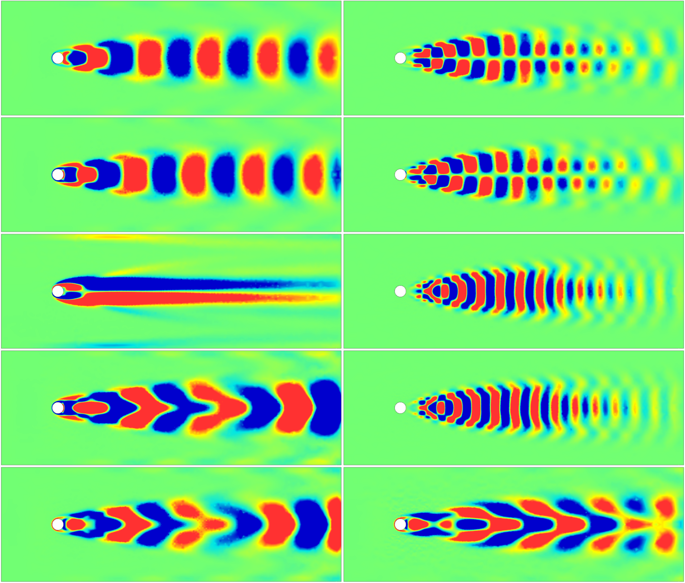
Figure 7: Same as figure 3 but for the first ten RDMD modes.

Figure 8: Same as figure 4 but for the first ten RDMD modes.

The first ten RDMD modes are depicted in figure 7. Intriguingly, RDMD resolves the first harmonics (modes $i=1,2$), the second harmonics ($i=6,7$) and the third harmonics ($i=8,9$). The associated mode amplitudes show corresponding oscillations starting near zero and reaching asymptotic values on the limit cycle. Mode 3 shows a nearly pure shift mode, describing the transition of the base flow from the steady solution to the time-averaged flow. In contrast to Noack et al. (2003), the amplitude becomes negative, since the sign of the RDMD mode is arbitrary. Modes 4 and 5 resolve intermediate vortex shedding patterns with maximum activity around $t=70$ and rather small residual fluctuations on the limit cycle. Modes 10 and 11 (not shown) are reminiscent of stability eigenmodes and peak near $t=55$, i.e. more than two periods earlier.

The first seven modes have significant similarities with the POD modes of figures 3 and 4. Yet, the oscillations are more symmetric (compare RDMD and POD mode 6) and show no apparent frequency mixing, as in POD modes $i=3,6,8$. RDMD modes have by definition a lower averaged residual, as compared to POD modes, but they look much cleaner and even reveal the third harmonics. It appears that the RDMD modes have more in common with POD than with DMD modes. This should not come as a surprise, since the primary construction principle is the minimization of the residual while the secondary criterion is the emulation of single-frequency DMD-mode behaviour.

4.4 Comparison of POD, DMD and RDMD

In this section, results from POD, DMD and RDMD are quantitatively compared.

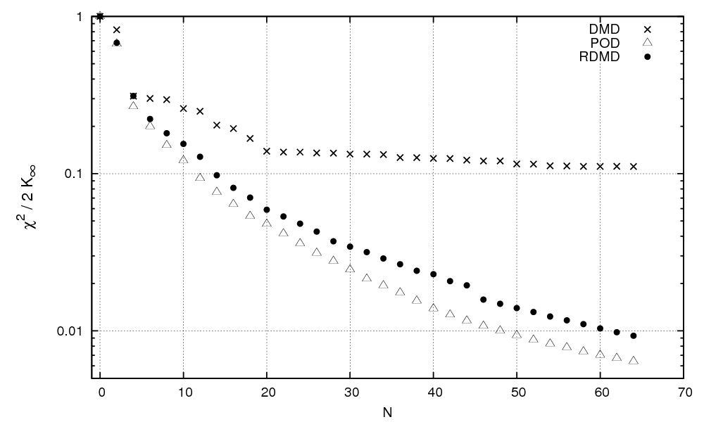
Figure 9: The time-averaged fluctuation level of the residual (10) for POD, DMD and RDMD with increasing number of modes. The value is normalized by the corresponding fluctuation level ($2K_{\infty}$) on the limit cycle.

Figure 10: The instantaneous normalized truncation error (10) as a function of time for 10 POD, DMD and RDMD modes. The figure displays the sampling interval.

Figure 9 shows the truncation error of the POD, DMD and RDMD expansions as a function of the number of modes. As expected, all errors decrease monotonically with the number of modes and POD outperforms DMD and RDMD. The RDMD residual, however, follows the POD value remarkably well and stays within similar orders of magnitude. In contrast, DMD approaches an effective asymptote near $10\%$ of the final fluctuation level.

The temporal evolution of the instantaneous truncation error is displayed in figure 10 for POD, DMD and RDMD at $N=10$. The maximum value in $t\in[60,70]$ is lowest for POD and largest for DMD. RDMD performs, as expected, between the alternative expansions. A surprising feature are the asymptotes. POD and DMD have similar truncation errors near $10\%$ of the terminal fluctuation level while RDMD outperforms both with a final value at about $5\%.$ This is no contradiction to the optimal property of POD, as this property only guarantees a minimal time-averaged value, or, equivalently, a minimal value of the integral over the instantaneous truncation error, which it evidently has. The DMD-based frequency filtering included in RDMD appears to have ’anticipated’ the limit cycle behaviour. One indication of this ’anticipation’ is the third harmonics which is featured in RDMD but absent in both POD and DMD. At this stage, RDMD appears more suitable for reduced-order modeling when compared to POD or DMD. Like POD, RDMD yields orthonormal modes, but with purer frequency content. Like DMD, RDMD extracts oscillatory modes, but with well-defined initial and asymptotic behaviour of the mode amplitudes.

5 Conclusions

We propose a novel data-driven flow decomposition which combines the modal orthonormality and low truncation error $\chi^{2}$ (10) of POD with the frequency-distilling features of DMD. This decomposition is recursively defined. First, the data set is subjected to DMD, after which a normalized DMD mode is chosen which minimizes the averaged error $\chi^{2}$. This procedure is recursively repeated in the orthogonal subspace of computed modes. The resulting recursive DMD (RDMD) modes are orthonormal by construction and can be expected to have lower error $\chi^{2}$ than DMD modes while retaining the monochromatic features of DMD.

POD, DMD and RDMD have been applied to the same snapshots of a transient cylinder wake starting near the steady solution and terminating on the limit cycle. As expected, RDMD significantly outperforms DMD in terms of the maximum, time-averaged and asymptotic truncation error for all considered mode numbers by a large margin. In addition, the exponentially growing or decaying DMD amplitudes neither resemble initial nor asymptotic flow behaviour in a meaningful manner while RDMD amplitudes clearly identify initial, transient and post-transient flow phases.

Table 1: Comparison of POD, DMD and RDMD for the transient cylinder wake. The maximum and asymptotic truncation errors are for expansions with $N=10$ modes normalized with the post-transient fluctuation level $2K_{\infty}$.

Aspect	POD	DMD	RDMD
Ideal snapshots	uncorrelated	time-resolved	time-resolved
Averaged truncation error	optimal	poor	good
Maximum truncation error	13%	46%	28%
Asymptotic truncation error	10%	10%	5%
Modal frequency content	mixed	pure	almost pure
Noise sensitivity	low	high	like
		without filter	DMD
Niche applications	statistics	stability modes	transient
		Fourier modes	dynamics

Also as expected, RDMD modes have far purer frequency content than POD but maintain the residual at comparable level. While the maximum and average truncation error of POD outperforms RDMD, RDMD shows a better resolution of the limit cycle: the asymptotic value for $N=10$ is half as large as the corresponding POD value and the third harmonic frequency is only captured by RDMD. Table 1 provides a brief comparison of the main characteristics and features of POD, DMD and RDMD.

The literature contains alternative approaches for spectrally purified POD modes. One important recent contribution is spectral POD (Sieber et al., 2015) which interpolates between POD and DMD by filtering the correlation matrix. This continuous interpolation offers an additional degree of freedom not present in RDMD; the price is the loss of strict orthonormality of the modes for all interpolation parameters. In a similar vein, Bourgeois et al. (2013) construct orthogonal POD modes with purer frequency content after Morlet-filtering the flow data at design frequencies. RDMD can be considered as a simpler approach which can be expected to perform well in an unsupervised manner, but leaves little room for tuning the modes for special purposes or applications.

The current study indicates that RDMD is an attractive ’compromise’ between POD and DMD. It sacrifices little of the optimal residual property of POD while retaining the single-frequency behaviour of DMD. Its potential in control-oriented reduced-order modeling will be explored in a future effort. In addition, a particularly attractive opportunity for RDMD is the unsupervised extraction of generalized mean-field models with few dominant frequencies (Brunton & Noack, 2015).

References

- Bagheri (2013) Bagheri, S. 2013 Koopman-mode decomposition of the cylinder wake. J. Fluid Mechanics 726, 596–623.
- Barkley & Henderson (1996) Barkley, D. & Henderson, R.D. 1996 Three-dimensional Floquet stability analysis of the wake of a circular cylinder. J. Fluid Mech. 322, 215–241.
- Bergmann & Cordier (2008) Bergmann, M. & Cordier, L. 2008 Optimal control of the cylinder wake in the laminar regime by Trust-Region methods and POD Reduced Order Models. J. Comp. Phys. 227, 7813–7840.
- Bourgeois et al. (2013) Bourgeois, J. A. Martinuzzi, R. J. & Noack, B. R. 2013 Generalised phase average with applications to sensor-based flow estimation of the wall-mounted square cylinder wake. J. Fluid Mech. 736, 316–350.
- Brunton & Noack (2015) Brunton, S. L. & Noack, B. R. 2015 Closed-loop turbulence control: Progress and challenges. Appl. Mech. Rev. 67 (5), 050801:01–48.
- Chen et al. (2012) Chen, K. K., Tu, J. H. & Rowley, C. W. 2012 Variants of dynamic mode decomposition: Boundary condition, koopman, and fourier analyses. J. Nonlinear Sci. 22 (6), 887–915.
- Coats (1997) Coats, C.M. 1997 Coherent structures in combustion. Prog. Energy Combust. Sci 22, 427–509.
- Courant & Hilbert (1989) Courant, R. & Hilbert, D. 1989 Methods of Mathematical Physics, Volume 1. Hoboken: Wiley-VCH.
- Deane et al. (1991) Deane, A. E. Kevrekidis, I. G. Karniadakis, G. E. & Orszag, S. A. 1991 Low-dimensional models for complex geometry flows: Application to grooved channels and circular cylinders. Phys. Fluids A 3, 2337–2354.
- Fletcher (1984) Fletcher, C. A. J. 1984 Computational Galerkin Methods, 1st edn. New York: Springer.
- Föppl (1913) Föppl, L 1913 Wirbelbewegung hinter einen Kreiszylinder (transl.: vortex motion behind a circular cylinder),. Sitzb. d. k. bayr. Akad. d. Wiss. 1, 1–18.
- Galerkin (1915) Galerkin, B.G. 1915 Rods and plates: series occuring in various questions regarding the elastic equilibrium of rods and plates (translated). Vestn. Inzhen. 19, 897–908.
- Gerhard et al. (2003) Gerhard, J. Pastoor, M. King, R. Noack, B. R. Dillmann, A. Morzyński, M. & Tadmor, G. 2003 Model-based control of vortex shedding using low-dimensional Galerkin models. In 33rd AIAA Fluids Conference and Exhibit. Orlando, Florida, USA, June 23–26, 2003, paper 2003-4262.
- Han et al. (2013) Han, Z.-H.. Stefan, G. & Zimmermann, R. 2013 Improving variable-fidelity surrogate modeling via gradient-enhanced kriging and a generalized hybrid bridge function. Aerospace Sci. Techn. 25 (1), 177–189.
- Hoarau et al. (2006) Hoarau, C. Borée, J. Laumonier, J. & Gervais, Y. 2006 Analysis of the wall pressure trace downstream of a separated region using extended proper orthogonal decomposition. Phys. Fluids 18, 055107.
- Holmes et al. (1998) Holmes, P. Lumley, J. L. & Berkooz, G. 1998 Turbulence, Coherent Structures, Dynamical Systems and Symmetry, 1st edn. Cambridge: Cambridge University Press.
- Jørgensen et al. (2003) Jørgensen, B. H. Sørensen, J. N. & Brøns, M. 2003 Low-dimensional modeling of a driven cavity flow with two free parameters. Theoret. Comput. Fluid Dynamics 16, 299–317.
- von Kármán & Rubach (1912) von Kármán, T. & Rubach, H. 1912 Über den Mechanismus des Flüssigkeits- und Luftwiderstandes. Phys. Zeitschr. XIII, 49–59.
- Lorenz (1956) Lorenz, E.N. 1956 Empirical orthogonal functions and statistical weather prediction. Tech. Rep.. Technical report, MIT, Department of Meteorology, Statistical Forecasting Project.
- Lorenz (1963) Lorenz, E. N. 1963 Deterministic nonperiodic flow. J. Atm. Sci. 20, 130–141.
- Lugt (1995) Lugt, H.J. 1995 Vortex flow in nature and technology. Melbourne, FL, USA: Krieger Publishing Company.
- Lumley (1967) Lumley, J.L. 1967 The structure of inhomogeneous turbulent flows. In Atmospheric Turbulence and Wave Propagation (ed. A.M. Yaglom & V.I. Tatarski), pp. 166–178.
- Noack et al. (2003) Noack, B. R. Afanasiev, K. Morzyński, M. Tadmor, G. & Thiele, F. 2003 A hierarchy of low-dimensional models for the transient and post-transient cylinder wake. J. Fluid Mech. 497, 335–363.
- Noack et al. (2004) Noack, B. R. Pelivan, I. Tadmor, G. Morzyński, M. & Comte, P. 2004 Robust low-dimensional Galerkin models of natural and actuated flows. In Fourth Aeroacoustics Workshop, pp. 0001–0012. RWTH Aachen, Feb. 26–27, 2004.
- Oberleithner et al. (2011) Oberleithner, K. Sieber, M. Nayeri, C. N. Paschereit, C. O. Petz, C. Hege, H.-C. Noack, B. R. & Wygnanski, I. 2011 Three-dimensional coherent structures in a swirling jet undergoing vortex breakdown: Stability analysis and empirical mode construction. J. Fluid Mech. 679, 383–414.
- Orszag (1971) Orszag, S.A. 1971 Numerical simulation of incompressible flows within simple boundaries: accuracy. J. Fluid Mech. 49, 75–112.
- Rom-Kedar et al. (1990) Rom-Kedar, V. Leonard, A. & Wiggins, S. 1990 An analytical study of transport, mixing and chaos in unsteady vortical flow. J. Fluid Mech. 214, 347–394.
- Rowley et al. (2009) Rowley, C. W., Mezić, I. Bagheri, S. Schlatter, P. & Henningson, D.S. 2009 Spectral analysis of nonlinear flows. J. Fluid Mech. 645, 115–127.
- Schlegel et al. (2012) Schlegel, M. Noack, B. R. Jordan, P. Dillmann, A. Gröschel, E. Schröder, W. Wei, M. Freund, J. B. Lehmann, O. & Tadmor, G. 2012 On least-order flow representations for aerodynamics and aeroacoustics. J. Fluid Mech. 697, 367–398.
- Schmid (2010) Schmid, P. J. 2010 Dynamic mode decomposition for numerical and experimental data. J. Fluid. Mech 656, 5–28.
- Schumm et al. (1994) Schumm, M. Berger, E. & Monkewitz, P.A. 1994 Self-excited oscillations in the wake of two-dimensional bluff bodies and their control. J. Fluid Mech. 271, 17–53.
- Sieber et al. (2015) Sieber, M., Oberleithner, K. & Paschereit, C. O. 2015 Spectral proper orthogonal decomposition. Tech. Rep. 1508.04642 [physics.fui-dyn]. arXiv.
- Siegel et al. (2008) Siegel, S. G. Seidel, J. Fagley, C. Luchtenburg, D. M. Cohen, K. & McLaughlin, T. 2008 Low dimensional modelling of a transient cylinder wake using double proper orthogonal decomposition. J. Fluid Mech. 610, 1–42.
- Sirovich (1987) Sirovich, L. 1987 Turbulence and the dynamics of coherent structures, Part I: Coherent structures. Quart. Appl. Math. XLV, 561–571.
- Suh (1993) Suh, Y.K. 1993 Periodic motion of a point vortex in a corner subject to a potential flow. J. Phys. Soc. Jap. 62, 3441–3445.
- Taylor & Hood (1973) Taylor, Cedric & Hood, P 1973 A numerical solution of the navier-stokes equations using the finite element technique. Computers & Fluids 1 (1), 73–100.
- Williamson (1996) Williamson, C.H.K. 1996 Vortex dynamics in the cylinder wake. Annu. Rev. Fluid Mech. 28, 477–539.
- Zebib (1987) Zebib, A. 1987 Stability of viscous flow past a circular cylinder. J. Engr. Math. 21, 155–165.
- Zhang et al. (1995) Zhang, H.-Q. Fey, U. Noack, B. R. König, M. & Eckelmann, H. 1995 On the transition of the cylinder wake. Phys. Fluids 7 (4), 779–795.