Nature of phase transitions in Axelrod-like coupled Potts models in two dimensions

Abstract

We study $F$ coupled $q$-state Potts models in a two-dimensional square lattice. The interaction between the different layers is attractive, to favour a simultaneous alignment in all of them, and its strength is fixed. The nature of the phase transition for zero field is numerically determined for $F=2,3$. Using the Lee-Kosterlitz method, we find that it is continuous for $F=2$ and $q=2$, whereas it is abrupt for higher values of $q$ and/or $F$. When a continuous or a weakly first-order phase transition takes place, we also analyze the properties of the geometrical clusters. This allows us to determine the fractal dimension $D$ of the incipient infinite cluster and to examine the finite-size scaling of the cluster number density via data collapse. A mean-field approximation of the model, from which some general trends can be determined, is presented too. Finally, since this lattice model has been recently considered as a thermodynamic counterpart of the Axelrod model of social dynamics, we discuss our results in connection with this one.

I Introduction

Given a model of statistical mechanics whose thermodynamic behaviour and phase diagram are known, one can ask oneself what is the macroscopic behaviour that sets in when two or more such models are coupled together. For example, one motivation for this question could be to understand the effect of randomness, or, simply, the composed model could be interesting by itself. In general, when two or more models are coupled, the symmetry of a system and, consequently, its critical behaviour kardar ; goldenfeld ; stanley ; pathria , are altered. Even the phase transition nature may change. However, a priori it is not possible to say how dramatic these changes will be, or how sensitive they are to the choice of the inter-model coupling.

The $q$-state Potts model Potts52 ; Wu82 is a very popular lattice model which has been extensively studied within many different theoretical approaches. On the experimental side, systems from condensed matter obeying the same symmetry have been identified. For a two-dimensional square lattice geometry, it is known that a single $q$-state Potts model, in absence of external fields, undergoes a temperature-driven phase transition whose nature changes with $q$: it is continuous for $q\leq 4$ and abrupt for $q>4$. Concerning the critical behaviour, explicit forms have been conjectured for the thermal denNijs79 and magnetic Nienhuis82 exponents for $q\leq 4$, from which all the thermodynamic critical exponents can be derived. These conjectured values seem to be generally confirmed by numerical and perturbative approaches Wu82 . Besides the thermal behaviour, one can analyze the geometric one. The basic geometric object to consider in a lattice model is a cluster, a connected set of nearest neighbours in the same state. Varying the temperature, one typically observes that a geometrical phase transition, analogous to percolation, takes place stauffer ; fortunato02 . There are critical exponents associated with this transition too, and, in principle, they are independent of the thermal ones. In this line, for the Potts model, closed forms for the various fractal dimensions (bulk, surface, etc) of the infinite cluster at criticality have been obtained in LABEL:Vanderzande92.

In this work we study how the phase transition type and the critical behaviour of the $q$-state Potts model in a two-dimensional square lattice change when $F$ similar models (layers) are coupled. In particular, we adopt a four-point coupling of fixed strength between the layers. Our aim is to see how the known behaviour and the critical properties of the single-layer model are altered by the coupling.

Coupled Potts models have been discussed in the literature, mainly to get insight on a single model with random couplings Dotsenko99 . Matsuda Matsuda81 considered two Potts models coupled with a four-body interaction; in particular, he located the transition temperature in the two-dimensional case using self-duality arguments. Later, he generalized the study to many coupled layers for a Hamiltonian containing up to $2F$-point terms Matsuda83 . More recently, Dotsenko et al. Dotsenko99 considered the fixed-point structure and stability for a similar Hamiltonian to identify the corresponding conformal field theory. For the case $q=2$, our model is equivalent to the $F$-colour Ashkin-Teller (AT) model Ashkin43 ; Baxter ; Grest81 , which in two dimensions has been studied for a weak four-body coupling and generic $F$ in LABEL:Grest81 and in the limit $F\rightarrow\infty$ in LABEL:Fradkin1984. Throughout the article, we will make comparisons with previous results whenever possible.

Beyond its relevance for the field of critical phenomena, the study developed in this article is also motivated by a possible connection to a model of social dynamics. At the end of the 1990s, Axelrod introduced an agent-based vectorial model for the spread of social influence Axelrod97 . In this non-equilibrium model the agents live on a lattice and are characterized by a dynamical culture, a set of $F$ features each assuming values out of a finite set of $q$ traits. The interactions are local and act to increase the similarity between agents. Systematic quantitative studies of the Axelrod model have been performed, exploring different aspects: non-equilibrium phase transitions Castellano00 , the effects of noise Klemm03 ; Klemm05 , dimensionality Klemm03a and size finiteness Toral07 . Keeping in mind the delicacy of the connection between social and physical phenomena, thermodynamic (equilibrium) counterparts of the Axelrod model have been proposed Gandica13 ; Genzor14 . In particular, the Hamiltonian we analyze in this work coincides with that of LABEL:Gandica13, in which the authors focused on the one-dimensional case.

This article is organized as follows. In Sec. II we present the model and relate it to similar ones from statistical mechanics. Its possible connection to the Axelrod non-equilibrium model of social dynamics is briefly recalled too. In Sec. III a mean-field approximation is carried out, and the findings for phase transitions at this level are summarized. In the subsequent sections, we present the results of a numerical Monte Carlo study on a two-dimensional square lattice, for different choices of $F$ and $q$. In particular, in Sec. IV we analyze the phase transition type. For the cases $F=2,q=2$ and $F=3,q=2$, where continuous and weakly first-order phase transitions take place, respectively, we analyze in Sec. V the geometrical critical (or pseudocritical) behaviour and determine the fractal dimension of the incipient infinite cluster. Finally, Sec. VI is devoted to our conclusions.

II The model: $F$ coupled $q$-state Potts models, or, Thermodynamic Axelrod

Our model, as in LABEL:Gandica13, is constituted by $F$ coupled layers of $q$-state Potts models Potts52 ; Wu82 . The variable at the $i$th site of the lattice is an $F$-vector $\vec{\sigma}_{i}=(\sigma_{i1},\sigma_{i2},\dots,\sigma_{iF})$, and each of its components has $q$ possible values (we choose $0,1,\dots,q-1$). The Hamiltonian for $N$ sites in presence of an external field reads

$$\mathcal{H} = -\sum_{k=1}^{F}\sum_{\langle ij\rangle}J_{ij}\,\delta(\sigma_{ik},\sigma_{jk})-H\sum_{k=1}^{F}\sum_{i=1}^{N}\delta(\sigma_{ik},H_{k})~{},$$ (1)

$$\quad\text{where}\quad J_{ij}=\sum_{l=1}^{F}J~{}\delta(\sigma_{il},\sigma_{jl})\,,$$

$J>0$ and $H\geq 0$ are constants, and $\delta(\cdot\,,\cdot)$ is Kronecker’s delta. The symbol $\langle\cdot\rangle$ indicates nearest neighbour sites, and the sum is over distinct pairs. The quantities ${H_{k}}$ are the favoured directions selected by the external field. Rephrased in the language of the social Axelrod model, each agent, which may be seen as representing a person or a small village, is characterized by a dynamical culture, a set of ($F$) features each assuming values out of a finite set of ($q$) traits. The interaction in Eq. (1) is built to reproduce the Axelrod rules: the energy of a link decreases with the interaction strength (as it is common in Hamiltonian systems) and the interaction strength increases when the agents are aligned in the same direction. Besides similarities, there is an important difference between the original Axelrod model and this thermodynamic version: in the Axelrod model, the interactions between two agents stop when they are identical or completely different, and the dynamics leads to absorbing configurations. That is not the case in the thermodynamic version, where thermal fluctuations are present. In this sense, our model, which never gets frozen, should rather be compared with the Axelrod model in the presence of noise Klemm03 ; Klemm05 .

For the case of one layer ($F=1$), Eq. (1) reduces to the standard $q$-state Potts model. When more layers are present, our model is constituted by $F$ layers of $q$-state Potts models coupled via their energies (i.e., with a four-body term) Matsuda81 ; Dotsenko99 . When comparing with similar models, notice that ours contains only one coupling constant ($J$) and the ratio between the strengths of the two-body and four-body terms is fixed. This is clearly seen by rewriting Eq. (1) as follows

$$\mathcal{H}=-J\sum_{k=1}^{F}\sum_{\langle ij\rangle}\delta(\sigma_{ik},\sigma_{jk})-J\sum_{\begin{subarray}{c}k,l=1\\ k\neq l\end{subarray}}^{F}\sum_{\langle ij\rangle}\delta(\sigma_{ik},\sigma_{jk})\delta(\sigma_{il},\sigma_{jl})-H\sum_{k=1}^{F}\sum_{i=1}^{N}\delta(\sigma_{ik},H_{k}).$$ (2)

For the case $q=2$, our model is equivalent to the $F$-colour Ashkin-Teller model Ashkin43 ; Baxter ; Grest81 with (in Grest’s notation) a two-body coupling $K_{2}=\beta JF/2$, and the constraint $K_{4}/K_{2}=1/F$ between the two- and four- body couplings, as can easily be checked by rewriting Eq. (1) in terms of a spin-$\frac{1}{2}$ variable, assuming values $\pm 1$.

III Mean-Field approximation

In a Mean-Field (MF) approximation, an interacting system is replaced by independent constituents embedded in a modified environment. In our case, each agent, instead of interacting with its nearest neighbours, feels a uniform field, originated by the average orientation of the others. Many different recipes can be used to build such an approximation. In this section we present an approach constructed at the level of the probabilities for the various states LoicTurban ; Nishimori2011 .

III.1 Probabilities and variational method

In statistical mechanics, equilibrium averages of a generic quantity $A$ are obtained by taking into account all the possible microstates $\mu_{s}$, each with an appropriate weight $p(\mu_{s})$:

$$\langle A\rangle=\sum_{\mu_{s}}p(\mu_{s})A(\mu_{s})~{},$$ (3)

where the normalization condition $\sum_{\mu_{s}}p(\mu_{s})=1$ is satisfied. The specific form of the probabilities depends on the macroscopic constraints imposed on the system. We work in the canonical ensemble, where the weights are computed from the microscopic Hamiltonian ${\mathcal{H}}$ as $p(\mu_{s})=e^{-\beta{\mathcal{H}}(\mu_{s})}/Z$, and the normalization factor is the partition function $Z=\sum_{\mu_{s}}e^{-\beta{\mathcal{H}}(\mu_{s})}$. As usual, $\beta=1/k_{B}T$ is the inverse temperature, and $k_{B}$ the Boltzmann’s constant. All the thermodynamics can be extracted from the partition function $Z$, through its relation to the Gibbs free energy $G$, namely $G=-k_{B}T\ln{Z}$.

Consider now a generic probability $p_{0}$: the following inequality can be easily shown

$$G\leq G_{0}=\langle\mathcal{H}\rangle_{0}+k_{B}T\langle\ln p_{0}\rangle_{0}=E_{0}-TS_{0}~{},$$ (4)

where $\langle\dots\rangle_{0}$ denotes the averages computed using the probability $p_{0}$. The average energy $E_{0}=\langle{\mathcal{H}}\rangle_{0}$ and the statistical entropy $S_{0}=-k_{B}\langle\ln p_{0}\rangle_{0}$, both obtained using $p_{0}$, have been introduced too. Eq. (4) shows that any free energy $G_{0}$ computed in this way will be larger than the exact Gibbs free energy. In the spirit of variational methods, a form is proposed for $p_{0}$, which will depend upon a number of parameters; the best approximation to the exact free energy is then obtained minimizing $G_{0}$ with respect to these parameters.

In a MF approximation, the system is treated at a single-particle level. Therefore, the probability function factorizes into $N$ terms, one for each site,

$$p(\vec{\sigma_{1}},\dots,\vec{\sigma_{N}})\simeq\prod_{i=1}^{N}p_{i}(\vec{\sigma_{i}})~{}\quad\text{(MF approximation)}.$$ (5)

We underline that in this approach the full Hamiltonian is used; there are other MF approaches in which, instead, the simplifications are done at the level of the Hamiltonian Nishimori2011 . In general, the physical results are the same.

III.2 Mean-field approximation for the Thermodynamic Axelrod model

We present in this section the MF approximation of our model Eq. (1). The calculations are done for a lattice of generic dimensionality and geometry, and coordination number $z$, since this is the only lattice property affecting the MF results. In App. A we give a more detailed derivation for the case of one layer ($F=1$).

For symmetry reasons all the features behave in the same way, then the average occupation of the trait $\alpha$ for the feature (=layer) $k$ is

$$\langle\delta(\sigma_{ik},\alpha)\rangle=\left\{\begin{array}[]{l}\mu,\quad\text{if}\quad\alpha=0,\forall k\\ \nu,\quad\text{if}\quad\alpha\neq 0,\forall k~{}.\end{array}\right.$$ (6)

In the latter we have used translational invariance, and, without loss of generality, imagined that the external field favours the trait $0$ in any feature ($H_{k}=0,\forall k$). Of course, $\mu$ and $\nu$ are related by the constraint $\mu+(q-1)\nu=1$. It is convenient to define as an order parameter

$$m=\mu-\nu~{}\quad\quad\text{(MF order parameter)}:$$ (7)

as $T\rightarrow 0$, we expect $\mu=1$ and $\nu=0$, then $m=1$; as $T\rightarrow\infty$, we expect $\mu=\nu=1/q$, then $m=0$.

In MF approximation, we assume that the full probability factorizes into $N\times F$ terms

$$p_{MF}(\vec{\sigma_{1}},\dots,\vec{\sigma_{N}})=\prod_{i=1}^{N}p_{i}(\vec{\sigma_{i}})=\prod_{i=1}^{N}\prod_{k=1}^{F}p_{ik}(\sigma_{ik})~{}.$$ (8)

Notice that, with this choice, the different components at a site are not correlated. Throughout this study, both at the MF level and in the numerical simulations, we only distinguish between a (completely) ordered phase, in which all the components are ordered, and a disordered phase, in which they are all disordered. Phases in which the orientation is random within any layer, but at a single site the variables are correlated, are known to appear in the AT model when the four-body coupling is considerably larger than the one considered here Baxter ; Grest81 . For any layer we assume the following structure of the probability

$$p_{ik}(\sigma_{ik})=\frac{1+m[q\,\delta(\sigma_{ik},0)-1]}{q}~{},\quad\sigma_{ik}=0,1,\dots,q-1~{},$$ (9)

which is derived in detail for the $q$-state Potts model in App. A (see also LABEL:LoicTurban).

Defining $\Delta_{ij}=\left[\sum_{k=1}^{F}\delta(\sigma_{ik},\sigma_{jk})\right]^{2}$, one can rewrite the interaction term in Eq. (1) as $-J\sum_{\langle ij\rangle}\Delta_{ij}$. In view of the MF, is convenient to elaborate $\Delta_{ij}$ so that it becomes a product of terms, each depending on a single component at a site: using Eq. (24) it becomes

$$\Delta_{ij} = \sum_{\begin{subarray}{c}k,l=1\\ k\neq l\end{subarray}}^{F}\sum_{\alpha,\beta=0}^{q-1}\delta(\sigma_{ik},\alpha)\delta(\sigma_{jk},\alpha)\delta(\sigma_{il},\beta)\delta(\sigma_{jl},\beta)$$ (10)

$$+\sum_{k=1}^{F}\sum_{\alpha=0}^{q-1}\delta(\sigma_{ik},\alpha)\delta(\sigma_{jk},\alpha)~{}.$$

Taking the averages we get

$$\langle\Delta_{ij}\rangle_{MF}=\sum_{\begin{subarray}{c}k,l=1\\ k\neq l\end{subarray}}^{F}[\mu^{2}+(q-1)\nu^{2}]^{2}+\sum_{k=1}^{F}[\mu^{2}+(q-1)\nu^{2}]$$

$$=F(F-1)\left[\frac{1+m^{2}(q-1)}{q}\right]^{2}+F\left[\frac{1+m^{2}(q-1)}{q}\right]~{}.$$

The external field term at one site is simply $\langle\sum_{k=1}^{F}\delta(\sigma_{ik},H_{k})\rangle_{MF}=F\mu=F[1+m(q-1)]/q$ . For the statistical entropy, we must recall that now at any site we have $F$ variables, each of which can be in state $0$ or not. For symmetry reasons, we are only interested to know how many components are not in state $0$: all the others will be in state $0$. The number of ways of having $k$ of the $F$ components different from state $0$ is $\binom{F}{k}(q-1)^{k}$, the weight of each of them is computed as the product $\nu^{k}\mu^{F-k}$. As a check, notice that $\sum_{k=0}^{F}\binom{F}{k}(q-1)^{k}=q^{F}$, the total number of states for a site, as it should. One can directly write

$$\langle\ln{p_{MF}}\rangle_{MF}=$$ (12)

$$= N\sum_{k=0}^{F}\binom{F}{k}(q-1)^{k}~{}\nu^{k}~{}\mu^{F-k}\ln{\left(\nu^{k}~{}\mu^{F-k}\right)}$$

$$= N\frac{1}{q^{F}}\sum_{k=0}^{F}\binom{F}{k}(q-1)^{k}(1-m)^{k}\left[1+m(q-1)\right]^{F-k}$$

$$\times\ln\left\{\frac{(1-m)^{k}\left[1+m(q-1)\right]^{F-k}}{q^{F}}\right\}~{}.\quad\quad\quad$$

Combining all the contributions together we obtain the free energy per particle of Axelrod model in MF approximation

$$g_{MF}^{\text{Axelrod}}(m,T) \equiv \frac{G_{MF}}{N}=\frac{\langle\mathcal{H}\rangle_{MF}+k_{B}T\langle\ln{p_{MF}}\rangle_{MF}}{N}$$ (13)

$$= -\frac{Jz}{2}\left\{F(F-1)\left[\frac{1+m^{2}(q-1)}{q}\right]^{2}+F\left[\frac{1+m^{2}(q-1)}{q}\right]\right\}-HF\frac{1+m(q-1)}{q}$$

$$+\frac{k_{B}T}{q^{F}}\sum_{k=0}^{F}\binom{F}{k}(q-1)^{k}(1-m)^{k}\left[1+m(q-1)\right]^{F-k}\ln\left\{\frac{(1-m)^{k}\left[1+m(q-1)\right]^{F-k}}{q^{F}}\right\}~{}.$$

Notice that, as it should, Eq. (13) reduces to Eq. (A) in the case $F=1$.

III.3 Phase transitions at the mean-field level

Following the evolution of the global minimum of $g_{MF}^{\text{Axelrod}}(m,T)$ with the temperature, we can locate possible phase transitions and determine their type. In all the cases we analyzed, there is a transition from a low-temperature ordered phase ($m\neq 0$) to a high-temperature disordered one ($m=0$). For $F=1$ we reproduce the known result that the phase transition, at the mean-field level, is continuous for $q=2$ and abrupt for $q>2$ (see also App. A). For $F>1$, we find that the transition, at the mean-field level, is abrupt for any value of $q\geq 2$. Concerning the transition temperatures, we find the following systematics: for a given $F$, the transition temperature decreases as $q$ increases; for a given $q$, the transition temperature increases as $F$ increases. This can be understood as follows: increasing $q$ favours the entropic term, while increasing $F$ strengthens the interaction term (see Eq. (1)).

As representative examples, in Fig. 1

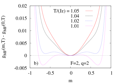
Figure 1: Free energy per particle of the thermodynamic Axelrod model in MF approximation, Eq. (13), for $H=0$, as a function of the order parameter $m$. (a) $F=1,q=2$; (b) $F=2,q=2$. In both cases, the function is shown for four values of the temperature in a range which encompasses the phase transition.

we show the mean-field free energy for the cases $F=1,q=2$ [Fig. 1(a)] and $F=2,q=2$ [Fig. 1(b)]. In the first one, a continuous phase transition takes place, whereas in the second one it is abrupt. This can be better seen in Fig. 2

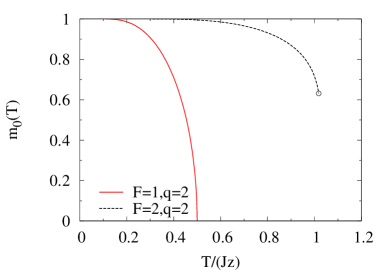
Figure 2: Physical value of the order parameter $m$ in the MF approximation [obtained as the global minimum of the free energy Eq. (13)], for $H=0$, as a function of the temperature, for the same two choices of $F$ and $q$ used in Fig. 1.

where the global minimum $m_{0}$ is shown as a function of the temperature and for the same two choices of $F$ and $q$.

Since at the MF level the fluctuations, whose strength is responsible for the singularities characterizing second-order phase transitions, are suppressed, it is natural to expect that some of the transitions appear abrupt at the MF level as an effect of the approximation.

IV Phase transition type

In this section we present our results for the phase transition type, obtained analyzing Monte Carlo simulations via the Lee-Kosterlitz method Lee90 ; Gould96 . Before discussing the results obtained for different choices of $F$ and $q$, we briefly recall the method used.

The Lee-Kosterlitz method allows to predict, from relatively small lattices, the nature of the phase transition taking place in the system in the thermodynamic limit. The central idea of this numerical approach is to monitor the evolution of the quantity $\Delta f(L)$, the height of the free energy barrier between two degenerate minima, as the system linear size, $L$, increases. If $\Delta f(L)$ increases with $L$, the transition is abrupt; if $\Delta f(L)$ is constant the transition is continuous; if $\Delta f(L)$ decreases there is no transition in the thermodynamic limit. The energy barrier is computed on a function $f(X,L)$ which is a restricted free energy, including only configurations which share the same value of the observable $X$, whose choice depends on the nature of the transition. For field-driven transitions, it is the order parameter ($X=M$), while for temperature-driven ones it is the energy ($X=E$). As usual, to reduce the computational costs, we use this method in combination with the histogram method by Ferrenberg and Swendsen Ferrenberg88 . The latter allows one to use a single Monte Carlo simulation at a given temperature to obtain estimates on the system thermodynamic quantities at temperatures nearby. Before going on, a warning is in order on the Lee-Kosterlitz method. While an increasing $\Delta f(L)$ is a (quite) safe proof of an abrupt phase transition, other cases are more tricky. In fact, the method relies on the behaviour of the energy barrier between two minima, but it can happen that this peak structure is not visible: in such a case, the transition may be continuous, or, it may be that the considered values of $L$ are too small to detect the barrier numerically, because the transition is weakly abrupt Kosterlitz93 .

Next we briefly summarize the numerical recipe used for a generic magnetic model. One starts with a long simulation at a given temperature ($k_{B}T_{0}=1/\beta_{0}$) close to the expected transition temperature, and builds the double histogram $H_{0}(E,M;L)$, counting the realizations with energy $E$ and (scalar) magnetization $M$. With this, the two restricted free energies are obtained as

$$f(E,\beta;L)=-\ln[\sum_{M}H_{0}(E,M;L)e^{-(\beta-\beta_{0})E}]~{},$$ (14)

and

$$f(M,\beta;L)=-\ln[\sum_{E}H_{0}(E,M;L)e^{-(\beta-\beta_{0})E}]~{}.$$ (15)

In the latter, we have included $\beta$ explicitly and written $f$ as a function of three variables. For the sake of clarity in the text and in the plots, when there is no ambiguity, we use the compact notation $f(E)$ and $f(M)$ to indicate these quantities.

For field-driven transitions, one fixes the temperature and lattice size, and measures the barrier height between degenerate minima in the function $f(M,\beta;L)$ (corresponding to ordering along different directions). The procedure is repeated for lattices of different sizes and a set of temperatures. Instead, for temperature-driven transitions, for any size $L$, one looks for the temperature at which $f(E,\beta;L)$ has two degenerate minima (corresponding to ordered and disordered phases). The barrier height between these minima is computed for different sizes.

We now come to our results. We have performed a numerical Monte Carlo study of the Hamiltonian (1) in a two-dimensional square lattice with periodic boundary conditions, using the Metropolis algorithm. The lattices are $L\times L$, with $N=L^{2}$ sites. A common definition of the order parameter to be used in simulations for the $q$-state Potts model is Challa86

$$m_{MC,F=1}=\frac{qx_{maj}-1}{q-1}~{},$$ (16)

where $x_{maj}$ is the average fractional occupation of the majority state. For a generic $F$, we use a similar definition

$$m_{MC}=\frac{q^{F}x_{maj}-1}{q^{F}-1}~{},$$ (17)

where the number of states is now $q^{F}$, since a state is a vectorial quantity. In this case, the MF definition and the Monte-Carlo one are slightly different: in fact, here we compare the occupations of vectorial states whereas in MF we compare the occupations of two traits in a feature. In the following we will denote with $M_{maj}$ the random variable whose thermal average per particle gives $m_{MC}$.

The values of $\beta_{0}$ we use to build the histograms are fixed according to Matsuda’s analytical predictions Matsuda81 for $F=2$ (see also App. B): $\beta_{c}J=0.333136$ for $q=2$, and $\beta_{c}J=0.401812$ for $q=3$, restricting to six decimal digits.

In Fig. 3,

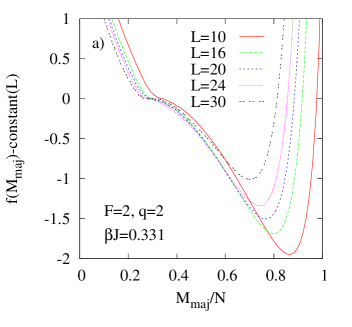
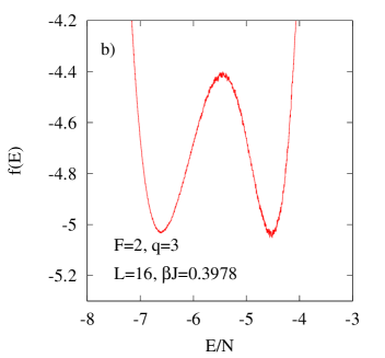
Figure 3: Example of the curves from which $\Delta f$ is extracted. (a) $f(M_{maj},\beta;L)$ for $F=2,q=2$, $\beta J=0.331$ and five values of $L$. The curves have been shifted vertically so that the inflection point is on the horizontal axis. (b) $f(E,\beta;L)$ for $F=2,q=3$, $\beta J=0.3978$ and $L=16$. In all the cases, $L\times L$ lattices are used, and $N=L^{2}$ is the total number of sites.

we show typical shapes of $f$: in Fig. 3(a), we give $f(M_{maj},\beta;L)$, for the case $F=2,q=2$, for five values of $L$ and a given temperature; in Fig. 3(b), we show $f(E,\beta;L)$, for the case $F=2,q=3$, for a given $L$ and temperature.

Let us focus on Fig. 3(a), $F=2,q=2$. Since at low temperature and in the absence of an external field there are $q^{F}$ degenerate states, in this case we expect four degenerate states. In this plot, obtained using the majority magnetization, the information about the direction of alignment is lost: the global minimum we see corresponds to ordering, in any direction. To distinguish between orientations in different directions, we could use a bi-dimensional order parameter: this variable would show indeed four degenerate minima, but the calculation of the free energy barrier between them would be very complicated. Instead, we identify the barrier in this case as the difference between the global minimum and the inflection point. At the same time, we take care that the run parameters and its length are such that all the degenerate minima are approximately equally visited during the simulation. As a test, we applied this recipe to case of a 3-state Potts model, and we could reproduce, a part from an irrelevant constant, the results of LABEL:Kosterlitz93.

From these and similar figures we extract $\Delta f$ in a range of temperature and sizes: the results for $F=2$ are summarized in Fig. 4,

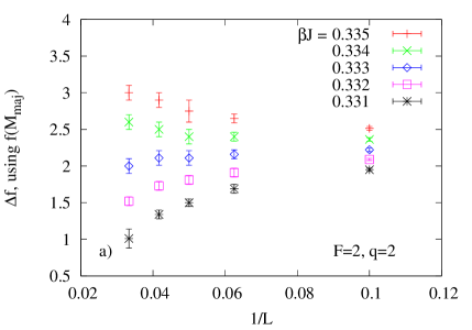
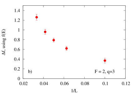
Figure 4: Free energy barrier $\Delta f$ as a function of the inverse of the lattice size $L$. (a) Case $F=2,q=2$, analysis of field-driven phase transitions. The barrier $\Delta f$ is obtained from $f(M_{maj},\beta;L)$, for a set of temperature values. The symbol shape denotes a given value of the temperature. (b) Case $F=2,q=3$, analysis of temperature-driven phase transitions. The barrier $\Delta f$ is obtained from $f(E,\beta;L)$. For each $L$ the barrier is computed at the temperature at which the two minima become (roughly) degenerate. In both panels, $L\times L$ lattices are used, with $L=10,16,20,24,30$.

it only remains to interpret them as explained above. For $F=2,q=2$, from Fig. 4(a) we see that a field-driven phase transition is abrupt for $\beta J>0.333$ and seems continuous for $\beta J\simeq 0.333$. Therefore, the temperature-driven phase transition at $\beta J\simeq 0.333$ appears continuous. For $F=2,q=3$, from Fig. 4(b) we deduce that the temperature-driven phase transition taking place at $\beta J\simeq 0.4$ is abrupt. Since we are interested in temperature-driven transitions, the reader may wonder why we do not use the approach of Fig. 4(b) also for $F=2,q=2$. The reason is simple: for $F=2,q=2$ we find a single minimum in the restricted free energy $f(E)$. While this is already an indication that no jump is present, so, if a transition occurs, it is probably continuous, we prefer to resort to another a point of view, that of $f(M)$, and apply the Lee-Kosterlitz method on it. As already discussed above, it is hard to distinguish, numerically, between a weakly first-order phase transition and a continuous one. What we can safely state is that the results of Fig. 4(a) are consistent with the presence of a continuous phase transition, and doing tests with $L$ up to $120$ we never saw the emergence of a peak in $f(E)$.

We repeat a similar analysis for the case of three coupled layers ($F=3$), and $q=2,3$. Unfortunately, for $F=3$ we do not have an analytical prediction for the transition temperature for the model, Eq. (1). In fact, analytical calculations based on duality arguments require the inclusion of six-point terms in the Hamiltonian in the case of three layers (see LABEL:Matsuda83). We then need to estimate the transition temperature: using a standard finite-size scaling study Gould96 ; Binder00 , we obtain $k_{B}T_{c}/J=4.9096(7)$ for $F=3,q=2$; for $F=3,q=3$, using the results on a $40\times 40$ lattice, we estimate $k_{B}T_{c}/J\simeq 4.06$. The results for $F=3$ are summarized in Fig. 5:

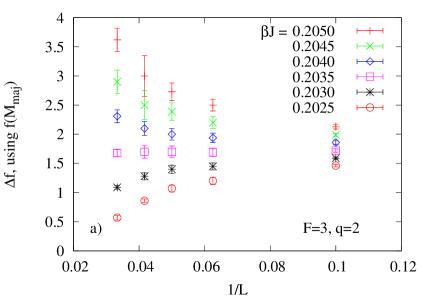
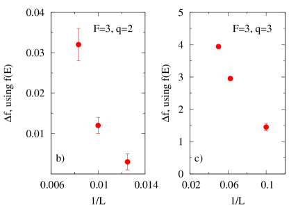
Figure 5: Free energy barrier $\Delta f$ as a function of the inverse of the lattice size $L$. (a) Case $F=3,q=2$, analysis of field-driven phase transitions. The barrier $\Delta f$ is obtained from $f(M_{maj},\beta;L)$, for a set of temperature values. The symbol shape denotes a given value of the temperature. Analysis of temperature-driven phase transitions for (b) $F=3,q=2$, and (c) $F=3,q=3$. The barrier $\Delta f$ is obtained from $f(E,\beta;L)$, as explained in Fig. 4. In all the panels, $L\times L$ lattices are used: in (a), $L=10,16,20,24,30$; in (b), $L=80,100,120$, and in (c), $L=10,16,20$.

the case with $q=2$ in Figs. 5(a) and 5(b) and the case with $q=3$ in Fig. 5(c). Again, we find that for $q=3$ an abrupt temperature-driven phase transition takes place [see Fig. 5(c)]. For $q=2$, and lattices of linear size $L$ up to $30$, we observe the same behaviour found for $F=2,q=2$ [compare Fig. 4(a) and Fig. 5(a)]. However, increasing the lattice size, we find that a two-minima structure develops in $f(E,\beta;L)$ for $L\geq 80$: in Fig. 5(b) we show the values of the energy barrier as a function of $1/L$. A comparison between Figs. 5(b) and 5(c) shows clearly that the phase transitions for $F=3,q=2$ and $F=3,q=3$, even if qualitatively similar, are quantitatively distinct: for $F=3,q=2$, where the phase transition is weakly abrupt, it is necessary to increase the lattice size by one order of magnitude to be able to see energy barriers which are two orders of magnitude smaller than in the case $F=3,q=3$.

Coming to the discussion of the results presented in this section, first of all, our findings for the phase transition type should be contrasted with the known result Wu82 that the $q$-state Potts model in a two-dimensional square lattice undergoes a continuous temperature-driven phase transition for $q\leq 4$ and an abrupt one for $q>4$. We find that the coupling of a layer with other ones (at least for the coupling considered here) results in a lowering of the value of $q$ for which the transition type changes from continuous to abrupt. Also, a comparison with the MF results shows that this approximation fails to catch the correct transition type only for $F=2,q=2$. Concerning the transition temperatures, they are, as usual, overestimated at the MF level, but the relative error gets smaller and smaller as the total number of states ($q^{F}$) increases. We mention that for the $q$-state Potts model it was conjectured that the MF approximation describes accurately the phase transition, in two or more spatial dimensions, when $q$ is large Mittag74 .

Second, we make a comparison with previous results available in the literature for coupled Potts models or similar ones. A summary of the expected nature of the temperature-driven phase transition in $F$ coupled $q$-state Potts models in a two dimensional square lattice can be found in LABEL:Pujol1996, and references therein. For an attractive coupling between the layers, as in our case, the transition type has been studied for different choices of $F$ and $q$: for $F=2$ and $q=2$, it is continuous Baxter (notice that, in this case, our model coincides with the Ashkin-Teller isotropic model, with a relative strength of the four-body term fixed to $K_{4}/K=1/2$, in Baxter notation); for $F=2$ and $q>2$, there are indications that it is abrupt Pujol1996 ; for $F>2$, and $q=2$, there are indications that it is abrupt (from LABEL:Grest81, which studies the $F$-colour AT model for weak four-body coupling); in the limit of $F\rightarrow\infty$ and $q=2$, it has been shown exactly that it is abrupt (from LABEL:Fradkin1984, which studies the $F$-colour AT model with a four-body coupling $\propto 1/F$). We recall here, as already discussed in Sec. III, that in the AT model new phases appear when the four-body interaction is larger than the one considered in this work Baxter ; Grest81 . The existence of a single phase-transition is also a necessary ingredient for Matsuda’s predictions based on self-duality: the agreement between our numerical results for the transition temperature and his prediction for $F=2$ confirms this point. More recently, in LABEL:Genzor14, Genzor et al. have shown results, obtained using the Corner Transfer Matrix Renormalization Group method, for our model, for $F=2$, $q=2,3$ (see Fig. 2 of that reference). While for $q=2$ their results for the transition temperature ($k_{B}T_{c}/J=3.0012$) and phase transition type are in agreement with ours and Matsuda’s ones, for $q=3$ they differ: in fact, in this case they find $k_{B}T_{c}/J=2.5676$ (Matsuda prediction, shown up to four decimal digits, is $2.4887$) and a continuous temperature-driven phase transition.

Finally, keeping in mind the differences between equilibrium and non-equilibrium models, we would like to recall at this point that for the non-equilibrium Axelrod model, in the absence of noise, an order-disorder phase transition is also found. In this case, it takes place as the number of traits $q$ is varied, at a value $q_{c}(F)$, and the type of the phase transition changes with $F$: it is continuous for $F=2$ and abrupt for larger $F$ Castellano00 . When noise (the temperature counterpart in this kind of models) is added to the original Axelrod model, continuous order-disorder transitions controlled by the noise rate are found in finite systems Klemm03 . A pseudo-critical noise rate $r_{c}$ at which the system behaviour changes can be identified Toral07 : for $r>r_{c}$ the system is disordered, while for $r<r_{c}$ it tends to a mono-cultural state. The quantity $r_{c}$ depends on the system size $N$, in a way that depends on the lattice properties; for a regular two-dimensional network, it is $r_{c}\approx 1/N\ln N$. Therefore, in the limit of infinite size $(N\rightarrow\infty$) the system is disordered as soon as $r\neq 0$. On the other side, in our thermodynamical version, that refers to infinite systems, we always find phase transitions. Therefore, in contrast with the one-dimensional case Gandica13 , in two spatial dimensions the thermodynamical version of the Axelrod model and the out-of-equilibrium original model with noise show a different qualitative behaviour when $N\rightarrow\infty$.

In the following section, we will address the geometrical properties of the system, showing that data collapse can be obtained in the continuous phase transition ($F=2,q=2$), but also in the weakly first-order one ($F=3$, $q=2$).

V Percolation critical behavior

At the critical point, as a consequence of the divergence of the correlation length, important simplifications take place in the thermodynamic properties, and lead to a universal (in the sense of the renormalization group) thermodynamic behaviour kardar ; goldenfeld ; stanley . Moreover, remarkably, in lattice spin models also some geometrical properties are characterized by interesting simplifications stauffer ; christensen . The divergence of the correlation length causes a power-law dominance, in terms of the relevant scale, in the cluster’s statistics functional form, in the vicinity of the critical point stauffer ; christensen ; fortunato02 .

In this Section we study the finite-size scaling of the cluster distribution in our model, to give a geometrical point of view on the phase transitions analyzed in the previous section. Since for the geometrical properties one faces the same difficulties discussed above in discriminating between a continuous phase transition and a weakly first-order one Peczak89 , we consider here both the $F=2,q=2$ and $F=3,q=2$ case. For the latter, in which an abrupt phase transition takes place, it is intended that the behaviour is only pseudo-critical, and the related exponents are pseudocritical as well. We focus on geometrical clusters, that is, sets of nearest neighbour sites in the same state, and indicate with $s$ the number of sites belonging to the cluster, also called the cluster mass. The cluster number density $n(s,T;L)$ gives the average number of clusters of size $s$ that is found at a temperature $T$ in a lattice $L\times L$, divided by the total number of sites. The finite-size scaling ansatz for the cluster number density at the critical point, $n(s,T_{c};L)$, states that christensen

$$n(s,T_{c};L)\propto s^{-\tau}\phi(s/L^{D}),\quad L\gg 1,s\gg 1~{},$$ (18)

where the function $\phi$ contains the information about the decay of the cluster number density for sizes bigger than the correlation length. The constants $\tau$ and $D$ are the Fisher critical exponent and the fractal dimension of the incipient infinite cluster (i.e., the largest cluster at $T=T_{c}$, also called the percolating cluster at $T=T_{c}$), respectively, and are related by the hyperscaling law

$$\tau=\frac{d}{D}+1~{},$$ (19)

where $d$ is the spatial dimensionality. Eq. (18) implies that we can collapse the curves for the cluster number density corresponding to lattices of different sizes, if we plot the transformed cluster number density, $s^{\tau}n(s,T_{c};L)$, against the rescaled cluster size, $s/L^{D}$ christensen .

Since $\tau$ can be obtained from $D$ using Eq. (19), to perform the collapse we only need to determine the fractal dimension, $D$, of the percolating cluster at the critical temperature. For this, we measure how the percolating cluster fills the space when the correlation length diverges, in terms of the lattice linear size, $S_{\infty}\varpropto L^{D}$ christensen . In our calculations, we measure the mass of the percolating cluster by means of the size of the biggest cluster at $T_{c}$. One early signal related to the kind of phase transition is the error in the linear fit for the log-log plot in the determination of $D$. The cases $F=2,3$ and $q>2$ as well as $q>5$ in the Potts model give high values for the Asymptotic Standard Error. On the contrary, we get a very low Standard Error $(<0.2\%)$ when $q=2$ for $F=2$ and $3$. Again, for the considered lattice sizes, the phenomenology of $F=2,q=2$ and $F=3,q=2$ is similar. Using lattices of size up to $L=100$, we obtain for the fractal dimension the values $D=1.885(2)$ for $F=2$ and $D=1.882(2)$ for $F=3$. The corresponding values of the Fisher exponent are $\tau=2.061(2)$ and $\tau=2.063(2)$ for $F=2$ and $3$, respectively.

Figure 6: Data collapse for the cluster number density, at $T=T_{c}$, for sizes $L=40$, $60$ and $80$. (a)-(c) The critical case $F=2,q=2$ and (d)-(f) the pseudo-critical case $F=3,q=2$. We show (a) and (d) the raw data for the cluster number density $n(s)$ against $s$, (b) and (e) the raw data for the transformed cluster number density $s^{\tau}n(s,T_{c};L)$ against $s$, and (c) and (f) the binned version of the transformed cluster number density $s^{\tau}n(s,T_{c};L)$ against the rescaled argument $s/L^{D}$.

In Fig. 6 we show the construction of the data collapse for the cluster number density as a function of the cluster size, for two values of $F$ and $q=2$. The critical case $F=2$ is shown in the top panels and the pseudo-critical case $F=3$ is given in the bottom panels. Figures 6(a) and 6(d) show the raw data for the cluster number density, i.e, the normalized cluster size distribution against $s$, for $L=40,60$ and $80$. The scale invariance over more than $5$ order of magnitude is evident and one can notice, at the same time, the appearance of the incipient infinite clusters (at larger sizes). Figures 6(b) and 6(e) display the transformed cluster number density $s^{\tau}n(s,T_{c};L)$ against the cluster size, $s$. Then, the onset of the rapid decay is in the same vertical position. To achieve the data collapse, the clusters size should be rescaled by the characteristic cluster size, $s_{\xi}$, which goes as $\varpropto\xi^{D}$ in infinite systems christensen . However, when systems are finite, the lattice sizes are always less than the correlation length and hence limit the characteristic cluster size: as a consequence $s_{\xi}\varpropto L^{D}$. Figures 6(c) and 6(f) depict the binned data for the collapse of the curves once the rescaling of the horizontal axis $s\rightarrow s/L^{D}$ has also been performed, illustrating the perfect collapse. Moreover, our data collapse also confirms the value of the critical exponent $\tau$, and of $D$.

Finally, we recall that for the case $F=1,q=2$ (2-state Potts model), the value of $D$ predicted by Vanderzande Vanderzande92 is $187/96=1.9479\dots$: we find therefore that when coupling two or three layers the fractal dimension $D$ is altered. The results for $F=2$ and $F=3$, however, are compatible within their error bars. As a test, we also compute $D$ for the case $F=1$, and in our simulations we get $D=1.9458(8)$, which agrees with the prediction by Vanderzande up to the second decimal. This indicates that the errors from the fits, which we have given in parenthesis, underestimate the real error, which is most likely in the second decimal digit. However, even with a conservative estimate of the error, our findings on the variation of $D$ are confirmed: $D=1.89$ for $F=2$, while $D=1.95$ for $F=1$. For $L$ up to $100$, $F=3$ has a pseudo-critical behaviour with $D=1.88$.

VI Conclusions

We have presented in this work a study of $F$ coupled $q$-state Potts models in a two dimensional square lattice, with an attractive four-body inter-layer coupling of fixed strength. We have analyzed the nature of phase transitions as the number of internal degrees of freedom $q$ and the number of layers $F$ are varied. Using the Lee-Kosterlitz method, we have found that the temperature-driven phase transition in zero field is continuous for $F=2,q=2$ and abrupt for higher values of $q$ and/or $F$. At mean-field level, we have found that for $F\geq 2,q\geq 2$ all the zero-field phase transitions are abrupt. This effect is a typical consequence of the suppression of fluctuations, whose strength is responsible for the singularities that characterize second-order phase transitions. However, the mean-field approximation has indicated the general dependence of the transition temperature upon $F$ and $q$, confirmed by MC results. The accuracy of the MF predictions for these temperatures improves as the total number of states ($q^{F}$) increases.

For $F=2,q=2$ and $F=3,q=2$, we have studied the properties of the geometrical clusters at the critical point, via finite-size scaling and data collapse. This has allowed us to determine the fractal dimension of the percolating cluster, showing that, when two layers are coupled, this fractal dimension is reduced from $D\simeq 1.95$ to $D\simeq 1.89$. When three layers are coupled, a pseudo-critical behaviour is found, with $D\simeq 1.88$.

We have made comparisons with previous results from the field of statistical mechanics, and, also, with the results obtained for the Axelrod model of social dynamics, a non-equilibrium model with some similar characteristics. In contrast with the one-dimensional case, in two spatial dimensions we have found that the thermodynamical version of the Axelrod model and the out-of-equilibrium original model with noise show a different qualitative behaviour in the limit of infinite size. This comparison is an example of the possible interesting connections that can be drawn between statistical mechanics and complex systems.

Appendix A Mean-Field approximation for $F=1$ — The q-state Potts model

We present here, closely following LABEL:LoicTurban, the MF approximation for the simple case of one layer, on which the case of generic $F$ is based. The calculations are done for a generic lattice, with coordination number $z$. The Hamiltonian (1) reduces in this case to the $q$-state Potts model

$$\mathcal{H}_{\text{Potts}}=-J\sum_{\langle ij\rangle}\delta(n_{i},n_{j})-H\sum_{i}\delta(n_{i},0)~{},$$ (20)

where $n_{i}=0,1,\dots,q-1$. Without loss of generality, we have assumed that the state $0$ is the favored one. We need to define two quantities: the probability $p({n_{i}})$ that a given site is in the state $n_{i}$, and the order parameter variable $s({n_{i}})$, whose average will describe the phase transition. The averages at one site $i$ are computed as $\langle A\rangle_{i}=\sum_{n_{i}=0}^{q-1}p(n_{i})A(n_{i})$.

In a MF approximation, the whole probability factorizes as

$$p_{MF}(n_{1},n_{2},\dots,n_{N})=\prod_{i=1}^{N}p_{i}(n_{i})~{}.$$ (21)

We make the following Ansatz: the single-site probability is $p(n_{i})=a+b\,\delta(n_{i},0)$ and $s(n_{i})=c+d\,\delta(n_{i},0)$, where $a,b,c,d$ are constants. The parameters $a$ and $b$ are fixed normalizing the probabilities ($\sum_{n_{i}=0}^{q-1}p(n_{i})=1$) and imposing that the average of the order parameter is $m$. The parameters $c,d$ are found imposing that $\langle s\rangle_{i}=1$ for $T=0$, and $\langle s\rangle_{i}=0$ for high temperatures.

One finds:

$$p(n_{i})=\frac{1+m[q\,\delta(n_{i},0)-1]}{q}~{},\quad n_{i}=0,1,\dots,q-1.$$ (22)

and

$$s(n_{i})=\frac{q\,\delta(n_{i},0)-1}{q-1}~{},\quad n_{i}=0,1,\dots,q-1.$$ (23)

To better understand the meaning of the quantity $m$, notice that it is the difference between the average occupation of state $0$ and of a state different from state $0$. In fact: the average occupation of state $0$ is $\mu\equiv\langle\delta(n_{i},0)\rangle_{i}=\frac{1+m(q-1)}{q}=m+\frac{1-m}{q}$ and for state $1$ (and any state other than $0$) it is $\nu\equiv\langle\delta(n_{i},1)\rangle_{i}=\frac{1-m}{q}$. Clearly, $\mu-\nu=m$.

Using the following exact relation

$$\delta(n_{i},n_{j})=\sum_{\alpha=0}^{q-1}\delta(n_{i},\alpha)\delta(n_{j},\alpha)~{},$$ (24)

we rewrite the Hamiltonian in a form which allows to evaluate directly the averages over single sites

$$\langle\mathcal{H}_{\text{Potts}}\rangle_{MF}=$$

$$= -J\sum_{\langle ij\rangle}\sum_{\alpha=0}^{q-1}\langle\delta(n_{i},\alpha)\rangle_{i}\langle\delta(n_{j},\alpha)\rangle_{j}-H\sum_{i}\langle\delta(n_{i},0)\rangle_{i}$$

$$= -J\frac{Nz}{2}[\mu^{2}+(q-1)\nu^{2}]-NH\mu$$

$$= -J\frac{Nz}{2q}[1+(q-1)m^{2}]-\frac{NH}{q}[1+m(q-1)]~{}.$$

In the above equality we have used the relation $\mu^{2}+(q-1)\nu^{2}=[1+m^{2}(q-1)]/q$ that one obtains rewriting $\mu$ and $\nu$ in terms of $m$.

For the statistical entropy term we have:

$$\langle\ln{p_{MF}}\rangle_{MF} = \sum_{i=1}^{N}\langle\ln{p_{i}}\rangle_{i}=\sum_{i=1}^{N}\sum_{n_{i}=0}^{q-1}p(n_{i})\ln{p(n_{i})}$$

$$= N\left[\mu\ln{\mu}+(q-1)\nu\ln{\nu}\right]$$

$$= N\bigg{\{}\frac{1+m(q-1)}{q}\ln\frac{1+m(q-1)}{q}$$

$$+(q-1)\frac{1-m}{q}\ln{\frac{1-m}{q}}\bigg{\}}~{}.$$

Finally, the Gibbs free energy per particle of the $q$-state Potts model in the MF approximation is

$$g_{MF}^{\text{Potts}}(m,T) \equiv \frac{G_{MF}}{N}=\frac{\langle\mathcal{H}_{\text{Potts}}\rangle_{MF}+k_{B}T\langle\ln{p_{MF}}\rangle_{MF}}{N}$$

$$= -J\frac{z}{2q}[1+(q-1)m^{2}]-\frac{H}{q}[1+m(q-1)]$$

$$+k_{B}T\bigg{\{}\frac{1+m(q-1)}{q}\ln\frac{1+m(q-1)}{q}$$

$$+(q-1)\frac{1-m}{q}\ln{\frac{1-m}{q}}\bigg{\}}~{}.$$

Analytical results for the MF approximation

For this $F=1$ case, analytical results for the transition temperature and type can be obtained at the MF level Wu82 . The inverse transition temperature $K_{c}=J/k_{B}T_{c}$ is

$$K_{c}z=2\frac{q-1}{q-2}\ln{(q-1)}$$ (26)

and the jump in the order parameter at transition is

$$m_{c}=\frac{q-2}{q-1}~{}.$$ (27)

The latter equation shows that at the MF level the phase transition is continuous for $q=2$ and abrupt for $q>2$.

Appendix B Previous exact results for the two-dimensional square lattice

Using self-duality arguments, the transition temperature of our model on a square lattice has been previously located for $F=1$ (Potts model, see, e.g. Wu82 ) and for $F=2$ Matsuda81 .

For $F=1$ and generic $q$, our model is a standard $q$-state Potts model whose transition in a square lattice is located solving

$$e^{K_{c}}=1+\sqrt{q}\Leftrightarrow K_{c}=\ln(\sqrt{q}+1)~{},\quad(F=1).$$ (28)

For $F=2$, generic $q$, and no external field, our model is equivalent to Matsuda’s model Matsuda81 with an appropriate choice of couplings. In more detail, our $J$ is related to $J_{i}$, $i=1,2,3$ of LABEL:Matsuda81 as follows: $J_{1}=J_{2}=J$ and $J_{3}=2J$. The transition temperature is found Matsuda81 by solving

$$e^{4K_{c}}-2e^{K_{c}}-(q-1)=0~{},\quad(F=2).$$ (29)

- (1) M. Kardar, Statistical Physics of Fields, Cambridge University Press, Cambridge (2007).
- (2) N. Goldenfeld, Lectures on Phase Transitions and the Renormalization Group, Perseus Books, Reading (1992).
- (3) H. E. Stanley, Introduction to phase transitions and critical phenomena, Clarendon Press, Oxford (1971).
- (4) R. K. Pathria, Statistical Mechanics, 2nd ed., Butterworth-Heinemann, Oxford (1996).
- (5) R. B. Potts, Proc. Cambridge Philos. Soc. 48, 106 (1952).
- (6) F. Y. Wu, Rev. Mod. Phys. 54, 235 (1982).
- (7) M. P. M. den Nijs, J. Phys. A 12, 1857 (1979).
- (8) B. Nienhuis, Phys. Rev. Lett. 49, 1062 (1982).
- (9) D. Stauffer and A. Aharony, Introduction to percolation theory, 2nd. ed., Taylor Francis, London (1994).
- (10) S. Fortunato, Phys. Rev. B 66, 054107 (2002).
- (11) C. Vanderzande, J. Phys. A 25, L75 (1992).
- (12) V. Dotsenko, J. L. Jacobsen, M.-A. Lewis, and M. Picco, Nucl. Phys. B 546, 505 (1999).
- (13) Y. Matsuda, Prog. Theor. Phys. 66, 2276 (1981).
- (14) Y. Matsuda, Physica A 117, 17 (1983).
- (15) J. Ashkin and E. Teller, Phys. Rev. 64, 178 (1943).
- (16) R. J. Baxter, Exactly solved models in Statistical Mechanics, Academic Press, London (1982).
- (17) G. S. Grest, M. Widom, Phys. Rev. B 24, 6508 (1981).
- (18) E. Fradkin, Phys. Rev. Lett. 53, 1967 (1984).
- (19) R. Axelrod, J. Conflict Resolut., 41, 203 (1997).
- (20) C. Castellano, M. Marsili, A. Vespignani, Phys. Rev. Lett. 85, 3536 (2000).
- (21) K. Klemm, V. M. Eguíluz, R. Toral, M. San Miguel, Phys. Rev. E 67, 045101(R) (2003).
- (22) K. Klemm, V. M. Eguíluz, R. Toral, and M. San Miguel, J. Econ. Dyn. Control 29, 321 (2005).
- (23) K. Klemm, V. M. Eguíluz, R. Toral, and M. San Miguel, Physica A 327, 1 (2003).
- (24) R. Toral, C. J. Tessone, Commun. Comput. Phys. 2, 177 (2007).
- (25) Y. Gandica, E. Medina, I. Bonalde, Physica A 392, 6561 (2013).
- (26) J. Genzor, V. Buzek, A. Gendiar, Physica A 420, 200 (2015).
- (27) L. Turban, Lecture notes on Physique Statistique, available on-line at http://gps.ijl.univ-lorraine.fr/webpro/turban.l/.
- (28) H. Nishimori and G. Ortiz, Elements of Phase Transitions and Critical Phenomena, Oxford University Press, New York (2011).
- (29) J. Lee, J. M. Kosterlitz, Phys. Rev. Lett. 65, 137 (1990).
- (30) H. Gould, J. Tobochnik, An introduction to computer simulation methods: applications to physical systems, 2nd ed., Addison-Wesley, New York (1996).
- (31) A. M. Ferrenberg, R. H. Swendsen, Phys. Rev. Lett. 61, 2635 (1988).
- (32) J. M. Kosterlitz, J. Lee, E. Granato, Springer Proc. Phys. 72, 28 (1993).
- (33) M. S. S. Challa, D. P. Landau, K. Binder, Phys. Rev. B, 34, 1841 (1986).
- (34) D. P. Landau and K. Binder, A Guide to Monte Carlo Simulations in Statistical Physics, Cambridge University Press, Cambridge (2000).
- (35) L. Mittag, M. J. Stephen, J. Phys. A 7, L109 (1974).
- (36) P. Pujol, Europhys. Lett. 35, 283 (1996).
- (37) K. Christensen and N. Moloney, Complexity and Criticality, Imperial College Press, London (2005).
- (38) P. Peczak, D. P. Landau, Phys. Rev. B 39, 11932 (1989).