Stationary bubbles and their tunneling channels toward trivial geometry

Abstract

In the path integral approach, one has to sum over all histories that start from the same initial condition in order to obtain the final condition as a superposition of histories. Applying this into black hole dynamics, we consider stable and unstable stationary bubbles as a reasonable and regular initial condition. We find examples where the bubble can either form a black hole or tunnel toward a trivial geometry, i.e., with no singularity nor event horizon. We investigate the dynamics and tunneling channels of true vacuum bubbles for various tensions. In particular, in line with the idea of superposition of geometries, we build a classically stable stationary thin-shell solution in a Minkowski background where its fate is probabilistically given by non-perturbative effects. Since there exists a tunneling channel toward a trivial geometry in the entire path integral, the entire information is encoded in the wave function. This demonstrates that the unitarity is preserved and there is no loss of information when viewed from the entire wave function of the universe, whereas a semi-classical observer, who can see only a definitive geometry, would find an effective loss of information. This may provide a resolution to the information loss dilemma.

I Introduction

Recently, there have been interesting discussions on the information loss problem of black holes Hawking:1976ra . It has been clearly exposed that one cannot consistently hold on to general relativity, semi-classical quantum field theory, area-entropy relation, and unitarity all at the same time Yeom:2008qw ; Almheiri:2012rt . This means that for a certain stage some of the well-established physical principles should breakdown, not only at singularities but also at very large scales. Among various ideas to address this problem, there is a proposal to drop general relativity introducing the so-called firewall Almheiri:2012rt . However, if there is a firewall, then it should affect the future infinity and hence that seems very problematic Hwang:2012nn ; CNOPSY .

An interesting approach to investigate this problem is via the wave function of the universe that satisfies the Wheeler-DeWitt equation Hartle:1983ai . If the universe is in the ground state, then the wave function can be computed by an Euclidean path-integral. One can approximate the path-integral as a sum over on-shell histories which are either Lorentzian or Euclidean, where the latter are called instantons. Namely an instanton is a classical trajectory over the complexified time that connects the initial state to one of the final states. For a given initial state, the wave function behaves as a propagator and the final state will be a superposition of various semi-classical states.

According to Maldacena Maldacena:2001kr and Hawking Hawking:2005kf , if one of the histories has a trivial topology, namely that there is no horizon nor singularity in the Lorentzian sense, then the information will be eventually conserved through the history, even though the probability is suppressed on the order of the entropy. This might explain why there is no information loss for the entire wave function of the universe, yet a semi-classical observer, who can see a definite geometry, would effectively detect the loss of information. It might well be that a unitary observer, if any, who lives in the superspace, could approximately describe classical observables as expectation values, where these expectation values do not have to satisfy the classical equations of motion. In this sense, there could be a violation of general relativity. But in this scenario there is no physical firewall for a semi-classical observer Sasaki:2014spa .

While this framework from the path-integral, so-called the effective loss of information, is very appealing, more justifications are needed. Possible issues of the effective loss of information are the following:

• Is the existence of an instanton that mediates a trivial geometry generic?

• Can one technically demonstrate the expectation values of observables in terms of a unitary observer?

• Is the existence of a trivial geometry really sufficient to explain unitarity?

If we can answer these questions positively, the effective loss of information will be a genuine answer for the information loss paradox.

In this paper, we want to address the first question: is the existence of such an instanton generic? Up to now, we are not yet able to answer this question, but we can at least find interesting and quite generic examples regarding this within the thin-shell approximation Sasaki:2014spa ; Lee:2015rwa . If a shell is self-gravitating and has a time-symmetric solution, then there is a hope to find a tunneling channel that links a collapsing shell to a bouncing shell toward a trivial geometry Farhi:1989yr . In order to obtain a trivial geometry within the thin-shell approximation, we need the following conditions:

• There should be time-symmetric collapsing and bouncing solutions.

• At the bouncing point, the extrinsic curvature of the shell should be positive.

• The shell should start with a regular initial condition and approach to a time-symmetric collapsing solution.

The existence of thin-shell solutions that satisfy C1 and C2 has already been shown in the literature Sasaki:2014spa ; Gregory:2013hja , while C3 was simply put in by hand. However, in order to make our argument more generic, we need to weaken these conditions. Regarding C3, for realistic star interiors, there exist various repulsive effects that can be well approximated by a modification of the tension term (for more detailed analytic descriptions of gravitational collapses, see Adler:2005vn ). In this paper, by modifying the tension around the star regime, we see that the realization of a regular initial condition that smoothly approaches a maximum radius is definitely reasonable and possible.

This paper is organized as follows. In SEC. II, we briefly summarize the idea on the effective loss of information. In SEC. III, we investigate true vacuum bubbles in asymptotic anti-de Sitter (AdS) and Minkowski backgrounds. We construct some examples that have stable or unstable stationary points by varying the tension term. Finally, in SEC. IV, we summarize our results and discuss on future topics. Some useful but supplementary analyses are given in Appendix. Throughout this paper, we assume the units $c=\hbar=G=1$, while in some special cases we explicitly recover the constants.

II Brief review on the effective loss of information

The propagator from the initial state $|i\rangle$ to the final state $|f\rangle$ can be described by the path integral

$$\langle f|i\rangle=\int\mathcal{D}g_{\mu\nu}\mathcal{D}\phi\;e^{iS[g_{\mu\nu},\phi]},$$ (1)

where $g_{\mu\nu}$ is the metric, $\phi$ is a matter field, and $S$ is the Lorentzian action. The final state, which is located at future infinity, is represented by a superposition of classical states $|f_{j}\rangle$, that is $|f\rangle=\sum_{j}a_{j}|f_{j}\rangle$, if one assumes the classicality of the wave function for an asymptotic observer.

In general, this Lorentzian path integral badly diverges. However, according to Hartle and Hawking Hartle:1983ai , an analytic continuation of the time from Lorentzian signatures to Euclidean signatures will improve its behavior and the analytically continued path integral will correspond to the ground state wave function. This Euclidean path integral is presented by

$$\langle f|i\rangle=\int\mathcal{D}g_{\mu\nu}\mathcal{D}\phi\;e^{-S_{\mathrm{E}}[g_{\mu\nu},\phi]},$$ (2)

where now $S_{\mathrm{E}}$ is the Euclidean action and we sum over all Euclidean paths that connect $|i\rangle$ to $|f_{j}\rangle$. Still, the whole path integral is difficult to solve exactly. Nevertheless, one can extract information about the ground state of the wave function by using the steepest-descent approximation, since in a semiclassical regime, Euclidean classical solutions (instantons) give the dominant contribution. In this approximation, one sums over instantons, namely

$$\langle f|i\rangle\simeq\sum_{i\rightarrow f_{j}}e^{-S^{\mathrm{on-shell}}_{\mathrm{E}}}.$$ (3)

Thus, the exponential gives a rough estimation on the tunneling rate from $|i\rangle$ to $|f_{j}\rangle$.

To be concrete, imagine a situation where the initial state defined on the past infinity $|i\rangle$ contains a collapsing matter that will classically form a black hole, and let us call it $|f_{\mathrm{BH}}\rangle$. Note that under the path integral approach, $|f_{\mathrm{BH}}\rangle$ will not be in general the unique final state; in other words, $|i\rangle$ may undergo quantum tunneling. Ideally, if there exists a history with a trivial geometry, say from $|i\rangle$ to $|f_{\cancel{\mathrm{BH}}}\rangle$, which has no singularity nor event horizon, then every information of the initial state $|i\rangle$ will be conserved through this history. In fact, this point was previously discussed by Maldacena Maldacena:2001kr and Hawking Hawking:2005kf . The main idea is as follows: although the probability for $|f_{\cancel{\mathrm{BH}}}\rangle$ is exponentially suppressed compared to $|f_{\mathrm{BH}}\rangle$, the two point correlation function between inside and outside the horizon does not decay to zero. Thus, information will be eventually recovered through the trivial geometry Maldacena:2001kr .

If this idea is general enough, then we might say that a unitary observer who can see the superposition of states $|f\rangle$ will restore all information, while a semiclassical observer will see a particular classical state, say $|f_{j}\rangle$, and will effectively lose information. This is the reason why this approach is called the effective loss of information. It should be noted that a unitary observer need not satisfy classical equations of motion (general relativity included).

Now, the question is whether the previous idea could be applicable for generic matter-gravity systems. We devote the following sections to find concrete examples where an instanton connects a collapsing matter to a trivial geometry.

III Dynamics and tunneling of true vacuum bubbles

We consider a spherical thin-shell located at $r$ that divides two spacetime regions with the spherical symmetric metric ansatz (for a review of the thin-shell formalism, see Toolkit )

$$ds_{\pm}^{2}=-f_{\pm}(R)dT^{2}+\frac{1}{f_{\pm}(R)}dR^{2}+R^{2}d\Omega^{2}\,,$$ (4)

where $\pm$ refer to outside ($R>r$) and inside ($R<r$) the shell, respectively. The intrinsic metric of the thin-shell is given by

$$ds^{2}=-dt^{2}+r^{2}(t)d\Omega^{2}.$$ (5)

We take the metric ansatz for outside and inside the shell to be

$$f_{\pm}(R)=1-\frac{2M_{\pm}}{R}+\frac{R^{2}}{\ell_{\pm}^{2}},$$ (6)

where $M_{+}$ and $M_{-}$ are the mass parameters of each region and

$$\ell^{2}_{\pm}=\frac{3}{8\pi\left|V_{\pm}\right|}$$ (7)

is the parameter due to the vacuum energy $V_{\pm}$. In this section, we focus on Minkowski and AdS background and consider true vacuum bubbles, but it can be easily generalized to a dS background. For our purposes we assume $M_{-}=0$, unless stated otherwise, and therefore the internal manifold does not have a singularity.

III.1 Junction equation and choice of tension

The equation of motion of the thin-shell is determined by the junction equation Israel:1966rt :

$$\epsilon_{-}\sqrt{\dot{r}^{2}+f_{-}(r)}-\epsilon_{+}\sqrt{\dot{r}^{2}+f_{+}(r)}=4\pi r\sigma\,,$$ (8)

where an overdot refers to the derivative with respect to the shell time $t$, $\epsilon_{\pm}=\pm 1$ denote the outward normal direction of outside and inside the shell, respectively, and $\sigma$ is the surface energy density or tension of the shell. It should be noted that the tension $\sigma$ is in general a function of $r$, which satisfies the conservation of the energy that is given by Blau:1986cw ; Ansoldi:1997hz :

$$\sigma^{\prime}=-\frac{2(\sigma+\lambda)}{r}\,,$$ (9)

where $\lambda$ is the surface pressure. The behavior of the tension with respect to $r$ is determined once an equation of state is given (for a study of the thin-shell dynamics in 2+1 dimensions for various equations of state see Mann:2006yu ). For example, if we assume a constant equation of state, i.e. $w\equiv\lambda/\sigma$, then we obtain

$$\sigma(r)=\frac{\sigma_{0}}{r^{2(1+w)}},$$ (10)

where $\sigma_{0}$ is a constant. In addition, if the shell is constructed by a couple of fields with various equations of state, then we can further generalize it as

$$\sigma(r)=\sum_{i=1}^{n}\frac{\sigma_{i}}{r^{2(1+w_{i})}},$$ (11)

where $\sigma_{i}$s are constants and $w_{i}$ corresponds equations of state.

The most natural realization of this model comes from a scalar field that gives the condition $w=-1$ (and hence a constant tension) Blau:1986cw . For the large $r$ limit, this gives the dominant contribution. However, for the small $r$ regime, there could be important contributions from other fields with different equations of states (e.g., Lee:2015rwa ).

III.2 Effective potential

After some calculations, we reduce the junction equation to a simpler formula Blau:1986cw :

$$\dot{r}^{2}+V(r) = 0,$$ (12)

$$V(r) = f_{+}(r)-\frac{\left(f_{-}(r)-f_{+}(r)-16\pi^{2}\sigma^{2}r^{2}\right)^{2}}{64\pi^{2}\sigma^{2}r^{2}}.$$ (13)

This effective potential determines the dynamics of the shell, where the classically allowed region is limited by $V(r)\leq 0$. Thus, the number of zeros of the potential especially determines the details. If there is no zero, then the only allowed solution is an asymmetric expanding or collapsing shell that connects between $r=0$ and $r=\infty$. However, if there are four zeros (FIG. 1), then these zeros would determine the turning points of the motion of the shell, i.e., where $\dot{r}=0$. Due to presence of these turning points, we find the following possibilities (FIG. 1):

• Symmetric collapsing solution: starting from $r=0$ at $t=-\infty$, approaching the turning point (maximum radius), and finally going to $r=0$ at $t=\infty$.

• Symmetric bouncing solution: starting from $r=\infty$ at $t=-\infty$, approaching the turning point (minimum radius), and finally going to $r=\infty$ at $t=\infty$.

• Oscillatory solution: oscillating between two turning points (a minimum and a maximum radius).

In addition, we add two extreme cases of the last possibility where two turning points merge into a single one (lower left and right of FIG. 1):

• Stable stationary solution: a solution where $V(r)=V^{\prime}(r)=0$ and $V^{\prime\prime}(r)<0$. Such a stationary solution is classically stable but will eventually either collapse or expand due to quantum effects.

• Unstable stationary solution: if $V(r)=V^{\prime}(r)=0$ and $V^{\prime\prime}(r)>0$, then the solution is stationary at a certain radius, but an infinitesimally small perturbation will induce either collapse or expansion; sometimes such a solution may be relevant as a thermal instanton Gomberoff:2003zh .

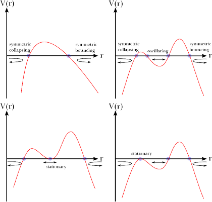
Figure 1: Examples of effective potentials, where there are two (upper left), three (lower), and four (upper right) zeros.

In this paper, we mainly focus on a tunneling channel corresponding to a bouncing solution that results in a trivial geometry without a singularity or an event horizon. Previously, several authors have found some examples Sasaki:2014spa , but these examples were associated with a symmetric collapsing solution. One potential problem with the symmetric collapsing solution is that it should start from $r=0$ and hence from a singularity and a white hole. It is reasonable to assume that such a region is not physical; if it does not have to satisfy the singularity theorem, then there can be a way to smoothen such an initial condition so that the initial state can be void of singularity.

On the other hand, the initial condition for the gravitational collapse of a real star is very complicated. To avoid such complications, we focus on the role of oscillatory and stationary solutions. These of course are not realistic models of gravitational collapse. Nevertheless, studying them is still meaningful in that it can explicitly deal with gravitational collapse geometries from regular initial configurations.

Our task is therefore to find a model where its effective potential $V(r)$ has four zeros to allow for symmetric collapsing solutions, symmetric bouncing solutions, and oscillating solutions; then as extreme cases, we can obtain a stable or unstable stationary solution.

Before going in depth, let us explicitly recover the signs of $\epsilon_{\pm}$ parameters by comparing extrinsic curvatures:

$$\beta_{\pm}(r)\equiv\frac{f_{-}(r)-f_{+}(r)\mp 16\pi^{2}\sigma^{2}r^{2}}{8\pi\sigma r}=\epsilon_{\pm}\sqrt{\dot{r}^{2}+f_{\pm}(r)}\,.$$ (14)

It is easy to see that whenever

$$\sqrt{f_{-}-f_{+}}>4\pi\sigma r\,,$$ (15)

$\beta_{+}$ is positive. We will make use of these fact in following sections.

III.3 Analysis of zeros

We dedicate this section to analyze the system and to build the previously discussed solutions. Essentially, we need to take into account two facts. First, the classification of solutions is directly related to the number of zeros of the potential. Second, the causal structure is determined by the sign of the extrinsic curvature. Thus, we are interested in the case when the potential has four zeros (or three zeros with one degenerate zero) and the extrinsic curvatures on both sides of the shell are positive for $r$ larger than the event horizon, i.e. $\epsilon_{\pm}=1$ for $r>r_{+}$ where $f_{+}(r_{+})=0$.

In other words, we want a stationary or oscillating thin-shell to tunnel to a trivial geometry with the resultant shell located at somewhere outside of the original shell and expanding to infinity, which is the one relevant to the future observer. Below, we first discuss how to tune the tension $\sigma$ so as to fulfill the above conditions. Then we present a couple of specific examples.

Solutions to $V(r)=0$ under the mentioned requirements are reduced to those satisfying

$$F(r)\equiv\sqrt{f_{-}}-\sqrt{f_{+}}=4\pi\sigma r.$$ (16)

Thus, if one looks for $n$ zeros, one must choose the tension $\sigma$ such that it satisfies Eq. (16) $n$ times. Let us have a rough intuition on the qualitative behavior of the function $F(r)$ in a near horizon, intermediate and far regions. We assume $\ell_{\pm}\gg M$ for simplicity. Near the event horizon $r\gtrsim r_{+}\sim 2M$, since we have $\ell_{\pm}\gg r$, we obtain

$$F(\ell_{\pm}\gg r) \simeq 1-\sqrt{\frac{r}{2M}-1}+\mathcal{O}\left(r^{3/2}\right)\,.$$ (17)

On the other hand, in the intermediate region where $\ell_{\pm}\gg r\gg M$, a series expansion yields

$$F(\ell_{\pm}\gg r\gg M) \simeq \frac{M}{r}+\mathcal{O}\left(r^{2}\right)\,.$$ (18)

Lastly, for large $r$, i.e. $r\gg\ell_{\pm}\gg M$, we obtain

$$F(r\gg\ell_{\pm}\gg M) \simeq \left(\frac{1}{\ell_{-}}-\frac{1}{\ell_{+}}\right)r+\mathcal{O}\left(r^{-1}\right)\,,$$ (19)

where it should be noted that the right-hand side is positive because $\ell_{-}<\ell_{+}$ for true vacuum bubbles. In this way, we have a crude idea on how $F(r)$ behaves and we can extract some conditions on the tension.

Before going into details, let us review the asymptotically flat case Sasaki:2014spa , namely $\ell_{+}=\infty$, and graphically explain the tension building as we base our intuition on this set up. First, by a simple analysis, it can be shown that in the asymptotically flat case one can always find a constant tension which yields two zeros of the potential. A necessary condition extracted from Eq. (19) is

$$\frac{1}{\ell_{-}}>4\pi\sigma_{0}\,.$$ (20)

For the asymptotically AdS case, we expect a similar condition on $\sigma_{0}$, namely

$$\frac{1}{\ell_{-}}-\frac{1}{\ell_{+}}>4\pi\sigma_{0}\,.$$ (21)

As seen explicitly from FIG. 2, a constant tension line (dashed black line) crosses $F(r)$ (red curve) twice, one in the large $r$ region and the other in the $\ell_{\pm}\gg r\gg M$ region where $F(r)$ starts to behave as $1/r$. Let us denote the positions of these two zeros by $r_{1}$ and $r_{2}$, where $r_{1}>r_{2}$. The blue curve shows the upper bound on $4\pi\sigma r$ so that the extrinsic curvature is positive at any $r$ greater than $r_{+}$ (see Eq. (15)). That ensures the presence of two zeros. In fact, since $\sqrt{f_{-}-f_{+}}\geq F(r)$ for $r\geq r_{+}$ and the equality holds only at the horizon, the existence of a zero in the large $r$ region guarantees that of another zero in the intermediate region.

Thus we first choose the constant part of the tension that satisfies Eq. (21). Afterwards, we modify the tension at $r<r_{2}$, around the $1/r$ region, so as to have the resulting curve (black curve) intersect the red curve two more times, as shown in FIG. 2. This can be achieved if one choose the tension to behave as $\sigma\sim 1/r^{\alpha}$ with $\alpha>2$ at $r<r_{2}$ and, hence, the product $\sigma r$ has a steeper gradient than $F(r)$ as $r$ decreases. This condition is equivalent to requiring the equation of state of the shell to cross the value $w=-1/2$, as one can see from evaluating

$$(\sigma r)^{\prime}=-\sigma(1+2w).$$ (22)

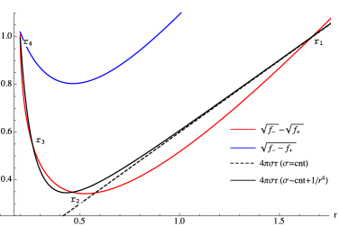
Figure 2: Qualitative behavior of $\sqrt{f_{-}}-\sqrt{f_{+}}$ (red), $\sqrt{f_{-}-f_{+}}$ (blue) and $4\pi\sigma r$ (black) for true vacuum bubbles in AdS background. A constant tension $\sigma$ (black dashed line) can give rise to two zeros of the potential at most. Four zeros could be obtained by modifying the tension at small $r$ (black line). The blue line sets the upper bound for the tension so as not to change the sign of the extrinsic curvature.

A concrete example: an unstable stationary thin-shell.

One can easily find an example that has an unstable stationary solution. Let us consider a tension given by

$$\sigma(r)=\sigma_{0}+\frac{\sigma_{1}}{r^{4}}\,,$$ (23)

where $\sigma_{0}$ ($w=-1$) is set from Eq. (21) and that the potential has two zeros as explained above. Therefore, we have to choose the contribution $\sigma_{1}$ from stiff matter ($w=1$) such that two more zeros at the small $r$ regime arise. Let us call the latter Model 1. FIGs. 4 and 4 show a particular example when $M=0.1$, $\ell_{-}=2$, $\ell_{+}=\infty$ and $4\pi\sigma_{0}=0.3$.

Concretely, the left panel of FIG. 4 shows $F(r)$ (red) and the upper bound on $4\pi\sigma r$ (blue) at small $r$. The two curves meet at the apparent horizon $r=0.2$. Here, we superimpose with black curves different values of $\sigma_{1}$, specifically $4\pi\sigma_{1}=0.006$ (bottom, dotted), $0.0067$ (curve) and $0.007$ (dashed).

In the critical limit where $4\pi\sigma_{1}=0.0067$, the potential has three zeros and hence it has a unstable stationary point. This can be clearly checked in terms of the effective potential (see FIG. 4). Additionally, the right panel of FIG. 4 confirms that the extrinsic curvatures are always positive for $r>r_{+}$.

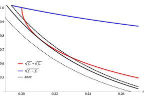
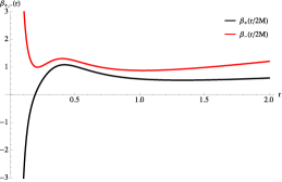
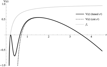
Figure 3: Left. $\sqrt{f_{-}}-\sqrt{f_{+}}$ (red) and $\sqrt{f_{-}-f_{+}}$ (blue) when $M=0.1$, $\ell_{-}=2$, $\ell_{+}=\infty$ and $4\pi\sigma_{0}=0.3$. $4\pi\sigma_{1}$ runs from $0.006$ (bottom, dotted), $0.0067$ (curve), $0.007$ (dashed), to $0.008$ (top, dotted). Right. The corresponding extrinsic curvatures $\beta_{+}$ (black) and $\beta_{-}$ (red) for $4\pi\sigma_{1}=0.0067$.

Figure 4: $V(r)$ for $M=0.1$, $\ell_{-}=2$, $\ell_{+}=\infty$, $4\pi\sigma_{0}=0.3$ and $4\pi\sigma_{1}=0.0067$. The dashed curve indicates the case when $\sigma_{1}=0$ and $f_{+}(r)$ (dotted line) is shown as a cross check that both extrinsic curvatures are positive for $r>r_{+}$.

A special case: thin-shell in pure vacuum background.

Let us turn our attention into the particular case when the vacuum energy in both inside and outside the shell vanishes, i.e. $\ell_{\pm}=\infty$. We are interested in building a classical stable thin-shell which may either tunnel to a black hole or expand to infinity leaving flat spacetime behind without any singularity. However, the foregoing discussion on true vacuum bubbles in asymptotically AdS background does not apply any longer as the function $F(r)$ approaches zero as $1/r$ in the limit $r\to\infty$ (see Eq. (18)). Thus, we need to tune the tension in a different way.

As $F(r)\propto 1/r$ for $r\to\infty$, the tension should decrease faster than $1/r^{2}$ to realize a zero at large $r$ (ie, for $4\pi\sigma r$ to cross $F$ from above). This requires $w>0$ as seen from Eq. (10). On the other hand, since $F\sim 1-\sqrt{(r-2M)/2M}$ near the horizon, any monotonically decreasing $\sigma$ which satisfies $8\pi M\sigma<1$ and $d(\sigma r)/dr<0$ at $r=2M$ would have a zero near the horizon (i.e., $4\pi\sigma r$ crosses $F$ from below), which requires $w>-1/2$.

The above consideration implies that there would be two zeros for a constant $w$ with $w>0$. However, we need two more zeros. This can be realized if we set $w$ sufficiently large near the horizon so that $\sigma r$ decreases faster than $F$ in a region slightly away from the horizon. Below we propose a model that satisfies these conditions.

The effective potential in the present case is given by

$$V(\bar{r})=1-\frac{1}{\bar{r}}-\frac{1}{4}\left({\frac{1}{\bar{\sigma}\bar{r}^{2}}}-\bar{\sigma}\bar{r}\right)^{2}\,,$$ (24)

where we normalized $r$ to the Schwarzschild radius, i.e. $\bar{r}=r/2M$, and defined $\bar{\sigma}\equiv 8\pi M\sigma$. In this way, the analysis is effectively independent of $M$. In this case, the requirement that the extrinsic curvatures are positive translates to

$$\bar{\sigma}^{2}\bar{r}^{3}<1.$$ (25)

This is fulfilled near the horizon, $\bar{r}\sim 1$, if $\bar{\sigma}<1$ and also in the large $r$ limit if $w>0$. Among many possibilities of tensions which fulfill these criteria, we consider the one which seems to be physically motivated as well as simple.

The model is as follows. When the thin-shell tunnels and expands to infinity, only radiation will reach the observer. So we may assume $w(\bar{r}\rightarrow\infty)=1/3$. On the other hand, as discussed in the above, the tension $\sigma$ must increase fast enough to stabilize the shell as $r$ decreases. Thus, we consider a shell that undergoes a phase transition to stiff matter as $r$ decreases, that is $w(\bar{r}\rightarrow 0)=1$. Furthermore, we assume the thin-shell is composed of dust matter in the intermediate region, i.e. $w=0$.

To realize the above behavior, let us propose

$$w(\bar{r})=\left\{\begin{array}[]{ccc}\frac{1}{2}\tanh\left[\mu_{1}\left(\bar{r}_{1}-\bar{r}\right)\right]+\frac{1}{2}&\quad\bar{r}<\bar{r}_{m}\\ \frac{1}{6}\tanh\left[\mu_{2}\left(\bar{r}-\bar{r}_{2}\right)\right]+\frac{1}{6}&\quad\bar{r}>\bar{r}_{m}\end{array}\right.,$$ (28)

where $\mu_{i}$ and $r_{i}$ control, respectively, the steepness and position of the transition, and $r_{m}$ is the matching radius in the dust region. Notice that if the two transitions are sufficiently far apart, i.e. $\bar{r}_{1}\ll\bar{r}_{m}\ll\bar{r}_{2}$, the matching is automatic and the exact value of the matching radius $r_{m}$ becomes irrelevant. Lastly, we set the tension as

$$\bar{\sigma}(\bar{r})=\bar{\sigma}_{0}\,\bar{r}^{-(2+2w(\bar{r}))}\,$$ (29)

where $\bar{\sigma}_{0}<1$. We note that because of the $\bar{r}$-dependence of $w$, it is no longer exactly equal to the ratio of the pressure to the energy density. Nevertheless, for sufficiently steep transitions $w$ is a good approximation to the pressure to the energy density ratio almost everywhere.

As a concrete model, we first choose $\bar{\sigma}_{0}<1$ so that the positivity of the extrinsic curvatures is guaranteed. Next we require that the transitions are fast enough, which roughly implies $\mu_{1}\gtrsim\mathcal{O}(1)$ and $\mu_{2}\gtrsim\mathcal{O}(1)$. Afterwards, we choose $\bar{r}_{1}$ and $\bar{r}_{2}$. Here we consider a set of models with various values of $\bar{r}_{1}$ which are not too large compared to unity and with a fixed value of $\bar{r}_{2}$ which is large enough so that the matching is smooth enough, i.e. $|\mu_{1}(r_{1}-r_{m})|\gg 1$ and $|\mu_{2}(r_{2}-r_{m})|\gg 1$. A particular example is shown in FIGs. 6 and 6 where we choose $\bar{\sigma}_{0}=0.99$, $\mu_{1}=1/2$, $\mu_{2}=1/5$ and $\bar{r}_{2}=40$. We refer to it as Model 2. If $\bar{r}_{1}=1.5$ then one has three zeros and, therefore, a stable stationary thin-shell.

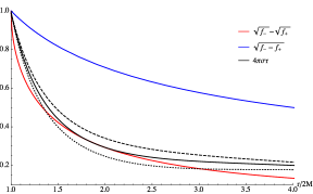
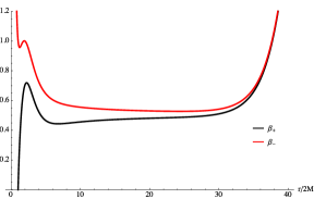
Figure 5: Left. $\sqrt{f_{-}}-\sqrt{f_{+}}$ (red), $4\pi\sigma r$ (black) of Model 2 when $\bar{\sigma}_{0}=0.99$, $\mu_{1}=1/2$, $\bar{r}_{1}=1.5$, $\mu_{2}=1/5$ and $\bar{r}_{2}=40$. The additional black lines are $\bar{r}_{1}=2$ (dotted) and $\bar{r}_{1}=1$ (dashed). It should be noted that by construction $4\pi\sigma r$ crosses again the curve $\sqrt{f_{-}}-\sqrt{f_{+}}$ and, therefore, the total number of zeros is three. Right. Extrinsic curvatures of Model 2, black for $\beta_{-}$ and red for $\beta_{+}$. Both of them are positive for $r>r_{+}$.

Figure 6: This figure shows $V(r)$ and $f_{+}(r)$. The shell is located in a local stable minimum and can either collapse or expand by tunneling effects. Notice that there is no point for $r>r_{+}$ where $V(r)=f_{+}(r)$ and, hence, the extrinsic curvatures are both positive.

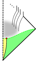
Figure 7: After summing over histories, we see the superposed geometry $\langle g_{\mu\nu}\rangle$.

III.4 Tunneling probability

Before ending this section, let us compute the tunneling probability for Model 2. As usual, in the Euclidean path integral approach, the probability is estimated semi-classically by the WKB approximation, that is

$$P\sim{\rm e}^{-B/\hbar}\,,$$ (30)

where $\hbar$ is the reduced Planck constant and

$$B=2\int_{r_{\times a}}^{r_{\times b}}|P_{\mathrm{E}}(r)|dr$$ (31)

is the integral of the Euclidean momentum of the shell between two consecutive zeros, $r_{\times a}$ and $r_{\times b}$, which is given by Ansoldi:1997hz

$$P_{\mathrm{E}}(r)=-r\cos^{-1}\left(\frac{f_{-}+f_{+}-(4\pi\sigma r)^{2}}{2\sqrt{f_{-}f_{+}}}\right)\,,$$ (32)

where $-\pi<\cos^{-1}<0$. In fact, due to the simplicity of our example in the pure vacuum background, we find that the probability is given by

$$\frac{B}{\hbar}=\frac{M^{2}}{M_{\mathrm{Pl}}^{2}}\frac{1}{\pi}\int_{\bar{r}_{\times a}}^{\bar{r}_{\times b}}|P_{\mathrm{E}}(\bar{r})|d\bar{r}\,,$$ (33)

where we have recovered the units and $M_{\mathrm{Pl}}$ is the reduced Planck mass ($=\sqrt{\hbar c/8\pi G}$). It should be noted that the integral is just a numerical value and that, for our choice of tension, a rough numerical approximation to the integral for the tunneling to a black hole and an expanding shell respectively gives

$$B_{\rm BH}\approx 0.3~{}{M^{2}}/{M_{\mathrm{Pl}}^{2}}\qquad{\rm and}\qquad B_{\rm expand}\approx 27.4~{}{M^{2}}/{M_{\mathrm{Pl}}^{2}}\,,$$ (34)

respectively. Note that the former is $100$ times small than the latter. This result agrees with the well believed fact that the tunneling probability is exponentially suppressed with the exponent of the order of the entropy. More explicitly, the ratio between probabilities for our case yields

$$\frac{P_{\rm expand}}{P_{\rm BH}}\sim{\rm e}^{-27.1{M^{2}}/{M_{\mathrm{Pl}}^{2}}}\,,$$ (35)

namely that the probability that the shell tunnels into a black hole is exponentially higher. Regarding the information loss paradox, if one thinks of this stable thin-shell as a quantum mechanical system, no actual issue arises. Basically, one has a wave packet which is located at the stable minimum of the potential and which will evolve and spread. Of course, the highest probability goes towards the formation of a black hole but there is spreading of the wave function for large $r$ as well. In this sense, there is no information loss.

Interestingly, in the limiting case where $M\sim\mathcal{O}(M_{\mathrm{Pl}})$, if we can give any physical meaning to it, the probability of an expanding solution is no longer exponentially suppressed and the superposition of geometries would start to be important, illustratively shown in FIG. 7. In any case, we have to bear in mind that this is a particular example and the conclusion depends on the choice of the tension. Nevertheless, this particular example could be considered as a model for gravitational stellar evolution where the most probable final stage is to form a black hole.

IV Conclusion

In this paper, we investigate stationary bubbles and their tunneling channels a trivial geometry. By tuning the tension of the shell under reasonable assumptions on the equation of state, we realize stationary solutions. These stable and unstable stationary shells could be a good toy model for a star interior around the time when gravitational collapse turns on. In this way, it can either collapse to a black hole or tunnel toward an expanding shell. For the latter case, even though the probability is exponentially suppressed, there will be no singularity nor event horizon, and hence information is conserved under the Euclidean path integral approach to the wave function of the universe.

What we achieved in this paper can be summarized as follows:

• In the time-symmetric solution, there is a part of the initial singularity and the white hole horizon. However, the initial singularity is not the essential feature; we can explicitly construct a model that does not start from an initial singularity.

• For realistic gravitational collapse, there can be much diverse (maybe, infinite number of) branching channels toward a trivial geometry, where each process will be exponentially suppressed with the exponent given by the order of the entropy $\sim M^{2}/M_{\rm Pl}^{2}$.

• We constructed a classically stable thin-shell example. In this case, the probability that forms a black hole and that expands to infinity will be both exponentially suppressed (though that depends on the tension). The two probabilities will be unsuppressed and of the same order when the mass becomes the Planck scale, i.e., when the “fuzziness” of the geometry becomes important.

We found various parameters that allow both collapsing and bouncing solutions. While this may not be the most general case, these parameters seem quite natural and therefore allowed. This suggests that we may go one step forward toward a generic behavior of the wave function of the universe. One must bear in mind that we are dealing with a broad class of examples but still it is no definite proof that there always exists an instanton that mediates a trivial geometry. However, if this generic statement were to be proven someday, then we might reach a solution to the information loss paradox through the Euclidean path integral approach.

Appendix: Causal structure and interpretation

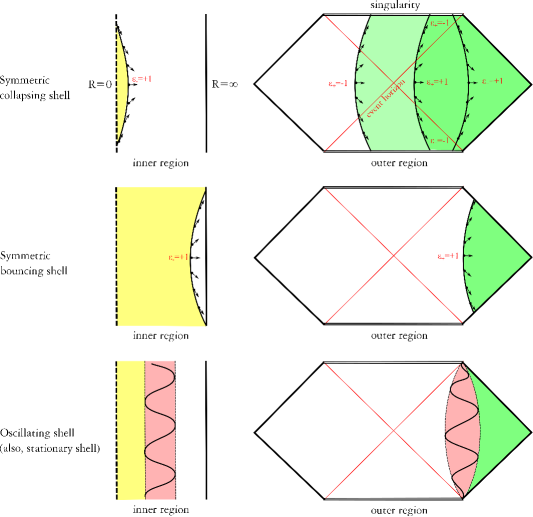
Figure 8: Causal structures of symmetric collapsing solutions (upper), symmetric bouncing solutions (middle), and oscillating solution (lower), where left is the inner AdS and right is the outer Schwarzschild (we can easily generalize to asymptotic AdS or dS).

In this appendix we give an illustrative interpretation of the causal structures of Model 1 and Model 2, see FIG. 8. For symmetric collapsing solutions, in Model 1, there are two kinds: either there exists a region where $\epsilon_{+}=+1$ or $\epsilon_{+}$ is always negative; in Model 2, always $\epsilon_{+}=+1$ and the trajectory should follow the condition. If the bubble is a true vacuum bubble and if there is a symmetric bouncing solution, then the only possible solution is $\epsilon_{\pm}=+1$. Finally, we are interested in an oscillatory solution that is located the right side of the causal patch. A stable stationary solution is a special case when the turning points are close each other.

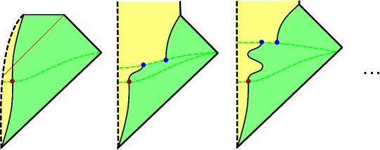
Figure 9: Left: an initial unstable shell begins to collapse and form a black hole (for Model 1). For Model 2, the shell will bend toward the left direction around the singularity. Middle: an initial unstable shell begins to bounce and tunnels toward a trivial geometry. Right: there can be various tunneling channels.

We can construct possible tunneling channels (FIG. 9) so-called Farhi-Guth-Guven/Fischler-Morgan-Polchinski tunneling Farhi:1989yr . This figure assumed the case when initially the shell was in the unstable local maximum. If the shell was in the stable local minimum, to trigger a formation of a black hole, one requires a tunneling and this will be easily generalized from FIG. 9. The unitary observer should superpose every histories (FIG. 7) Hartle:2015bna ; in terms of such an observer, the averaged metric $\langle g_{\mu\nu}\rangle$ can look like fuzzy that may not satisfy classical equations of motion (hence general relativity).

References

- (1) S. W. Hawking, Phys. Rev. D 14, 2460 (1976).
-
(2)
D. Yeom and H. Zoe,
Phys. Rev. D 78, 104008 (2008)
[arXiv:0802.1625 [gr-qc]];
S. E. Hong, D. Hwang, E. D. Stewart and D. Yeom, Class. Quant. Grav. 27, 045014 (2010) [arXiv:0808.1709 [gr-qc]];
D. Yeom and H. Zoe, Int. J. Mod. Phys. A 26, 3287 (2011) [arXiv:0907.0677 [hep-th]];
P. Chen, Y. C. Ong and D. Yeom, JHEP 1412, 021 (2014) [arXiv:1408.3763 [hep-th]]. -
(3)
A. Almheiri, D. Marolf, J. Polchinski and J. Sully,
JHEP 1302, 062 (2013)
[arXiv:1207.3123 [hep-th]];
A. Almheiri, D. Marolf, J. Polchinski, D. Stanford and J. Sully, JHEP 1309, 018 (2013) [arXiv:1304.6483 [hep-th]];
S. L. Braunstein, S. Pirandola and K. Zyczkowski, Phys. Rev. Lett. 110, no. 10, 101301 (2013) [arXiv:0907.1190 [quant-ph]]. -
(4)
D. Hwang, B. -H. Lee and D. Yeom,
JCAP 1301, 005 (2013)
[arXiv:1210.6733 [gr-qc]];
W. Kim, B. -H. Lee and D. Yeom, JHEP 1305, 060 (2013) [arXiv:1301.5138 [gr-qc]]. - (5) P. Chen, Y. C. Ong, D. N. Page, M. Sasaki and D. Yeom, arXiv:1511.05695 [hep-th].
- (6) J. B. Hartle and S. W. Hawking, Phys. Rev. D 28, 2960 (1983).
- (7) J. M. Maldacena, JHEP 0304, 021 (2003) [arXiv:hep-th/0106112].
-
(8)
S. W. Hawking,
Phys. Rev. D 72, 084013 (2005)
[arXiv:hep-th/0507171];
S. W. Hawking, arXiv:1401.5761 [hep-th]. - (9) M. Sasaki and D. Yeom, JHEP 1412, 155 (2014) [arXiv:1404.1565 [hep-th]].
-
(10)
B. H. Lee, W. Lee and D. Yeom,
Phys. Rev. D 92, no. 2, 024027 (2015)
[arXiv:1502.07471 [hep-th]];
J. Mas and A. Serantes, Int. J. Mod. Phys. D 24 (2015) 1542003 [arXiv:1507.01533 [gr-qc]]. -
(11)
E. Farhi, A. H. Guth and J. Guven,
Nucl. Phys. B 339, 417 (1990);
W. Fischler, D. Morgan and J. Polchinski, Phys. Rev. D 41, 2638 (1990);
W. Fischler, D. Morgan and J. Polchinski, Phys. Rev. D 42, 4042 (1990). -
(12)
R. Gregory, I. G. Moss and B. Withers,
JHEP 1403, 081 (2014)
[arXiv:1401.0017 [hep-th]];
P. Burda, R. Gregory and I. Moss, Phys. Rev. Lett. 115, 071303 (2015) [arXiv:1501.04937 [hep-th]];
P. Burda, R. Gregory and I. Moss, JHEP 1508, 114 (2015) [arXiv:1503.07331 [hep-th]]. - (13) R. J. Adler, J. D. Bjorken, P. Chen and J. S. Liu, Am. J. Phys. 73, 1148 (2005) [gr-qc/0502040].
- (14) E. Poisson, “A relativist’s toolkit: the mathematics of black-hole mechanics,” Cambridge University Press, 2004.
- (15) W. Israel, Nuovo Cim. B 44, 1 (1966) [Erratum-ibid. B 48, 463 (1967)].
- (16) S. K. Blau, E. I. Guendelman and A. H. Guth, Phys. Rev. D 35, 1747 (1987).
- (17) S. Ansoldi, A. Aurilia, R. Balbinot and E. Spallucci, Class. Quant. Grav. 14 (1997) 2727 [gr-qc/9706081].
- (18) R. B. Mann and J. J. Oh, Phys. Rev. D 74 (2006) 124016 [Phys. Rev. D 77 (2008) 129902] [gr-qc/0609094].
-
(19)
A. Gomberoff, M. Henneaux, C. Teitelboim and F. Wilczek,
Phys. Rev. D 69, 083520 (2004)
[hep-th/0311011];
J. Garriga and A. Megevand, Int. J. Theor. Phys. 43, 883 (2004) [hep-th/0404097]. -
(20)
J. Hartle and T. Hertog,
arXiv:1502.06770 [hep-th];
J. B. Hartle, arXiv:1511.01550 [quant-ph].