Neutron and proton electric dipole moments from $N_{f}=2+1$ domain-wall fermion lattice QCD

Abstract

We present a lattice calculation of the neutron and proton electric dipole moments (EDM’s) with $N_{f}=2+1$ flavors of domain-wall fermions. The neutron and proton EDM form factors are extracted from three-point functions at the next-to-leading order in the $\theta$ vacuum of QCD. In this computation, we use pion masses 0.33 and 0.42 GeV and 2.7 fm³ lattices with Iwasaki gauge action and a 0.17 GeV pion and 4.6 fm³ lattice with I-DSDR gauge action, all generated by the RBC and UKQCD collaborations. The all-mode-averaging technique enables an efficient and high statistics calculation. Chiral behavior of lattice EDM’s is discussed in the context of baryon chiral perturbation theory. In addition, we also show numerical evidence on relationship of three- and two-point correlation function with local topological distribution.

I Introduction

Electric dipole moments (EDM) are sensitive observables of the CP-violating (CPV) effects of the fundamental interactions described by the standard model (SM) and theories beyond the SM (BSM). The measurement of the neutron EDM (nEDM) has been attempted in experiments since the 1950’s; however no evidence for the nEDM has been found, and the latest experimental upper bound is tiny, $d_{N}\leq 2.9\times 10^{-26}$ e$\cdot$cm (90% CL)Baker et al. (2006, 2007). From the theoretical point of view, the contribution to the nEDM from the CPV phase in the CKM mixing matrix is extremely small since the first non-vanishing contribution appears at three loops, and $d_{N}\sim 10^{-31}$ e$\cdot$cm Mannel and Uraltsev (2013); Khriplovich and Zhitnitsky (1982); Khriplovich (1986); Czarnecki and Krause (1997), more than 5 orders of magnitude below the experimental bound. On the other hand, since the QCD Lagrangian contains a CP-odd $\theta$ term, the CPV effect from the strong interaction may dominate, even though its contribution appears to be unnaturally small, $d_{N}/\bar{\theta}\sim 10^{-17}$ e$\cdot$cm Crewther et al. (1979); Abada et al. (1991a); Aoki and Hatsuda (1992); Cheng (1991); Abada et al. (1991b); Pich and de Rafael (1991); Pospelov and Ritz (2000); Hisano et al. (2012); Borasoy (2000); Ottnad et al. (2010); Guo and Meissner (2012); O’Connell and Savage (2006); Kuckei et al. (2007); Mereghetti et al. (2011). This is known as the strong CP problem.

For search of the new physics due to BSM scenarios, nEDM is just about the most important observable, since naturalness arguments strongly suggest that BSM interactions will not be aligned with the usual quark mass eigenstates Agashe et al. (2005). As a consequence, in most BSM scenarios, there will be additional CP-odd phases, thus nEDM is a unique way to search the effect of these new phase(s). Extensions of the SM can generate nEDM at 1-loop order in the new interactions, for example Left-Right Symmetric models Beall and Soni (1981), extra-higgses models, warped models of flavor Agashe et al. (2005) and supersymmetric (SUSY) models  Abel et al. (2001); Hisano and Shimizu (2004); Ellis et al. (2008); Li et al. (2010); Ibrahim and Nath (2008); Fukuyama (2012). Indeed some of the most popular models, e.g. SUSY, have a problem that the expected size of nEDM value is bigger than existing bounds Engel et al. (2013). In fact, warped models which are considered extremely attractive for a geometric understanding of flavors, the nEDM naturally arises around the same level as the current experimental bound, so there is a mild tension by factors of a few. This means that if nEDM is not discovered after another order of magnitude improvement is made, then that will cause a serious constraint on the warped models of flavor. To extract BSM effects arising in an EDM, both high energy particle contributions and low energy hadronic effects have to be taken into account. Although there have been several estimates of BSM contributions to EDM’s, for instance from quark electric dipole, chromoelectric dipole, and Weinberg operators, based on effective models, baryon chiral perturbation theory (BChPT) and sum rules Pospelov and Ritz (2000); Hisano et al. (2012); Borasoy (2000); Ottnad et al. (2010); Guo and Meissner (2012); O’Connell and Savage (2006); Kuckei et al. (2007); Mereghetti et al. (2011); Bsaisou et al. (2015a, b); Mereghetti and van Kolck (2015), it is necessary to evaluate the unknown low-energy constants appearing in such models. On the other hand, computations from first principles using lattice QCD are also doable. A recent attempt at estimate of quark EDM contribution is given in Bhattacharya et al. (2015a, b).

This paper presents a first step in a feasibility study of the non-perturbative computation of nucleon EDM’s. The starting point is to perform the path-integral from an ab-initio calculation including the $\theta$-term. The renormalizability of the $\theta$-term allows a Monte-Carlo integration without considering the mixing with lower-dimensional CP violating operator. It is also an appropriate test for the next step towards inclusion of higher dimensional CP-odd sources associated with BSM theories. Currently there are three strategies for neutron and proton EDM computations in lattice QCD:

(1) Extraction of the EDM using an external electric field Aoki and Gocksch (1989); Aoki et al. (1990); Shintani et al. (2007, 2008); Shindler et al. (2015),

(2) Direct computation of the EDM form factor, in which the EDM is given in the limit of zero momentum transfer Shintani et al. (2005); Berruto et al. (2006); Alexandrou et al. (2015),

(3) Use of imaginary $\theta$ and extraction of the EDM as in (1) or (2). Izubuchi et al. (2007); Horsley et al. (2008); Guo et al. (2015)

In (1) the neutron and proton EDM are evaluated from the energy difference of nucleons with spin-up and spin-down in a constant external electric field. In Shintani et al. (2007, 2008) the calculation is carried out with Minkowskean electric field, with a signal appearing as a linear response to the magnitude of the electric field. However, as shown in Shintani et al. (2007, 2008), possibly large excited state contamination results due to enhanced temporal boundary effects of the Minkowskean electric field.

(2) is a straightforward method in which the EDM appears as the non-relativistic limit of the CP violating part of the matrix element of the the electromagnetic (EM) current in the ground state of the nucleon. It requires the subtraction of CP-odd contributions arising from mixing of the CP-even and odd nucleon states in the $\theta$-vacuum Shintani et al. (2005); Berruto et al. (2006). In this method, the EDM is obtained from the form factor at zero momentum transfer. This paper employs this strategy.

In (1) and (2), the $\theta$-term in Euclidean space-time is pure imaginary while the CP-even part of the action is real, which leads to a so-called sign problem for Monte-Carlo simulation. To avoid this issue, the idea of (3) is to employ a purely real action by using an imaginary value of $\theta$ in the generation of gauge field configurations. This has an advantage of improved signal-to-noise over the reweighting method. In Izubuchi et al. (2007); Horsley et al. (2008) preliminary results indicate relatively small statistical errors for the nEDM, however we note that these results may be affected by lattice artifacts due chiral symmetry breaking of Wilson-type fermions. Recently updated results in $N_{f}=2+1$ QCD using (3) have been presented in Ref. Guo et al. (2015) and appear promising.

Figure 11 (also see Shintani et al. (2012)) shows the summary plot of EDM results obtained using the strategies (1) and (3) and Wilson-clover fermions and strategy (2) using domain-wall fermions (DWF) which maintain chiral symmetry at non-zero lattice spacing to a high degree Furman and Shamir (1995). Older results suffer from large statistical errors and uncontrolled systematic errors. To pursue a more reliable estimate of the neutron and proton EDM’s, we adopt strategy (2) and use DWF. To efficiently reduce statistical errors we employ all-mode-averaging (AMA) Blum et al. (2013, 2012); Shintani et al. (2014).

This paper is organized as follows: in section II we introduce notation and give formulae used to extract the CP-even EM and CP-odd EDM form factors for the neutron and proton from correlation functions computed in lattice QCD. In section III we first describe the lattice setup, including AMA parameters, and then give numerical results for the EM and EDM form factors and subsequent neutron and proton EDM’s. We discuss our lattice QCD result in the context of phenomenological estimates in section IV and present an idea to further reduce statistical errors related to reweighting in section V. Finally we summarize our study in VI.

II Measurement of EDM form factor

II.1 Extraction of EDM form factor

The matrix element is parameterized similarly, with CP-even and odd form factors,

$$\langle N(\vec{p}_{f},s_{f})|V_{\mu}^{\rm EM}|N(\vec{p}_{i},s_{i})\rangle_{\theta}=\bar{u}_{N}^{\theta}(\vec{p}_{f},s_{f})\Big{[}F_{1}(q^{2})\gamma_{\mu}+\frac{iF_{2}(q^{2})}{2m_{N}}\frac{[\gamma_{\mu},\gamma_{\nu}]}{2}q_{\nu}$$

$$+\frac{F_{3}(q^{2})}{2m_{N}}\frac{\gamma_{5}[\gamma_{\mu},\gamma_{\nu}]}{2}q_{\nu}\Big{]}u_{N}^{\theta}(\vec{p}_{i},s_{i}).$$ (1)

where $F_{1}$ and $F_{2}$ are the usual CP-even EM form factors, and $F_{3}$ is the CP-odd EDM form factor. Here we focus on the electromagnetic interaction with quarks inside nucleon under $\theta$-vacuum, and so that $\langle\rangle_{\theta}$ is explicit representation of path-integral with $\theta$-term. $u_{N}^{\theta}$ denotes the nucleon spinor-function as a function of $\theta$. Each form factor is able to be extracted from order-by-order in $\theta$ in the expanded three-point function and Eq. (1) as shown below (also see Shintani et al. (2005); Berruto et al. (2006) for more detail). Note that momentum transfer $q=p_{f}-p_{i}$ is used in the space-like region.

We represent the three-point function in our lattice study as

$$C_{V_{\mu}}^{\theta}(t_{f},\vec{p}_{f};t,\vec{q};t_{i},\vec{p}_{i}) = C_{V_{\mu}}(t_{f},\vec{p}_{f};t,\vec{q};t_{i},\vec{p}_{i})$$ (2)

$$+ i\theta C_{V_{\mu}}^{Q}(t_{f},\vec{p}_{f};t,\vec{q};t_{i},\vec{p}_{i})+O(\theta^{2}),$$

where all terms on the RHS are computed in the $\theta=0$ vacuum, but the second is reweighted with topological charge $Q=\int G\tilde{G}/64\pi^{2}$ using gluon field strength $G$, in QCD action with $\theta$ term, $S_{\rm QCD}+i\theta Q$. Here the EM current is defined by the local bilinear, $V_{\mu}^{\rm EM}=Z_{V}\bar{q}\gamma_{\mu}Q_{c}q$ with quark charge matrix $Q_{c}={\rm diag}(2/3,-1/3,-1/3)$, as in the continuum theory, but multiplied by the lattice renormalization factor $Z_{V}$. In this paper, we ignore the SU_f(3) suppressed disconnected quark diagrams and compute only the connected part in three-point function.

We use the following ratio,

$$R_{\mu}(t_{f},\vec{p}_{f};t,\vec{q};t_{i},\vec{p}_{i})=K\frac{C_{V_{\mu}}(t_{f},\vec{p}_{f};t,\vec{q};t_{i},\vec{p}_{i})}{C_{G}(t_{f}-t_{i},\vec{p}_{f})}\bigg{[}\frac{C_{L}(t_{f}-t,\vec{p}_{i})C_{G}(t-t_{i},\vec{p}_{f})C_{L}(t_{f}-t_{i},\vec{p}_{f})}{C_{L}(t_{f}-t,\vec{p}_{f})C_{G}(t-t_{i},\vec{p}_{i})C_{L}(t_{f}-t_{i},\vec{p}_{i})}\bigg{]}^{1/2}$$ (3)

where $K=\sqrt{(E_{N}(\vec{p}_{f})+m_{N})(E_{N}(\vec{p}_{i})+m_{N})}/\sqrt{E_{N}(\vec{p}_{f})E_{N}(\vec{p}_{i})}$. The nucleon two-point function with smeared-source/smeared-sink is $C_{G}(t,\vec{p})$ and smeared-source/local-sink is $C_{L}(t,\vec{p})$. Taking the large time-separation limit to project onto the nucleon ground states,

$$\mathcal{R}_{\mu}(t_{f},\vec{p}_{f};t,\vec{q};t_{i},\vec{p}_{i})\equiv\lim_{t_{f}-t,t-t_{i}\rightarrow\infty}R_{\mu}(t_{f},\vec{p}_{f};t,\vec{q};t_{i},\vec{p}_{i})$$

$$=\sum_{s_{f},s_{i}}u_{N}^{\theta}(\vec{p}_{f},s_{f})\langle N(\vec{p}_{f},s_{f})|V_{\mu}|N(\vec{p}_{i},s_{i})\rangle_{\theta}\bar{u}_{N}^{\theta}(\vec{p}_{i},s_{i})$$

$$=\mathcal{R}_{\mu}(\vec{p}_{f},\vec{p}_{i})+i\theta\mathcal{R}^{Q}_{\mu}(\vec{p}_{f},\vec{p}_{i})+\mathcal{O}(\theta^{2}),$$ (4)

for the matrix element in (1).

To describe the RHS of (4) up to the second order in $\theta$, we replace the spinor sums by the matrix Shintani et al. (2005)

$$\sum_{s}u_{N}^{\theta}(\vec{p},s)\bar{u}^{\theta}_{N}(\vec{p},s) = E_{N}\gamma_{0}-i\vec{p}\cdot\vec{\gamma}+m_{N}e^{i\alpha_{N}(\theta)\gamma_{5}},$$ (5)

$$\approx E_{N}\gamma_{0}-i\vec{p}\cdot\vec{\gamma}+m_{N}(1+i\alpha_{N}(\theta)\gamma_{5})+\mathcal{O}(\theta^{2}),$$ (6)

where the CP-odd mixing angle $\alpha_{N}(\theta)$ induced by the $\theta$-term appears explicitly Here $\alpha_{N}(\theta)$ is a Lorentz scalar, thus it is as a function of quark mass. To the lowest order, $\alpha_{N}(\theta)\approx\theta\alpha_{N}$ is determined by

$${\rm tr}\Big{[}\gamma_{5}C_{L/G}^{\theta}(t,\vec{p})\Big{]}\simeq{Z^{*}}_{L/G}Z_{G}\frac{2m_{N}}{E_{N}}i\alpha_{N}\theta\big{(}e^{-E_{N}t}+(-)^{b}e^{-E_{N}(L_{t}-t)}\big{)},$$ (7)

in enough large $t$. $Z_{L/G}$ denotes normalization factor for local (L) or Gaussian smeared (G) sinks. $b$ indicates the boundary condition in the temporal direction with size $L_{t}$; $b=0$ is for periodic boundary conditions, and $b=1$ anti-periodic. $N^{*}$ denotes the parity partner of the nucleon in the $\theta=0$ vacuum. Note that to the order we are working, $Z$’s and $E$’s are given by the usual lowest order of $\theta$, CP-even quantities.

Using (6) and the definitions in (1), and taking traces with projectors $P_{4}^{+}\equiv(1+\gamma_{4})/2$ and $P_{5z}^{+}\equiv i(1+\gamma_{4})\gamma_{5}\gamma_{z}/2$, the leading order in $\theta$ ($\theta$-LO) form factors are obtained from (4) by

$${\rm tr}\Big{[}P_{5z}^{+}\mathcal{R}_{x}(0,\vec{p})\Big{]} = \frac{p_{y}}{E_{N}}G_{m}(q^{2}),$$ (8)

$${\rm tr}\Big{[}P_{5z}^{+}\mathcal{R}_{y}(0,\vec{p})\Big{]} = -\frac{p_{x}}{E_{N}}G_{m}(q^{2}),$$ (9)

$${\rm tr}\Big{[}P_{4}^{+}\mathcal{R}_{t}(0,\vec{p})\Big{]} = \frac{E_{N}+m_{N}}{E_{N}}G_{e}(q^{2}),$$ (10)

with Sachs electric and magnetic form factors

$$G_{e}(q^{2})=F_{1}(q^{2})-\frac{q^{2}}{4m_{N}}F_{2}(q^{2}),\quad G_{m}(q^{2})=F_{1}(q^{2})+F_{2}(q^{2}).$$ (11)

Similarly, including the $\alpha_{N}$ term in (6), the form factors appearing at next-to-leading order in $\theta$ ($\theta$-NLO) are obtained from

$${\rm tr}\Big{[}P_{5z}^{+}\mathcal{R}^{Q}_{t}(\vec{p}_{f},\vec{p}_{i})\Big{]} = i\frac{p_{z}}{2E_{N}}\bigg{[}\alpha_{N}\bigg{\{}F_{1}(q^{2})+\frac{3m_{N}+E_{N}}{2m_{N}}F_{2}(q^{2})\bigg{\}}-\frac{E_{N}+m_{N}}{m_{N}}F_{3}(q^{2})\bigg{]}.$$ (12)

The EDM form factors $F_{3}$ are then determined by the subtracting the $\alpha_{N}F_{1,2}$ terms.

III Numerical results

III.1 Lattice parameters

We use lattices with size $L_{\sigma}\times L_{t}=24^{3}\times 64$, Iwasaki gauge action with $a^{-1}=1.7848(6)$ GeV (gauge coupling is $\beta=2.13$) Aoki et al. (2011), and $L_{\sigma}\times L_{t}=32^{3}\times 64$, Iwasaki(I)-DSDR gauge action with $a^{-1}=1.3784(68)$ GeV (gauge coupling is $\beta=1.75$) Arthur et al. (2013). Both lattice scales were determined from a global, continuum and chiral fit Blum et al. (2014a), including physical point ensembles. The fermions are domain wall fermions (DWF), which significantly suppresses the $\mathcal{O}(a)$ lattice artifact due to chiral symmetry breaking. The additive quark mass shift from the explicit chiral symmetry breaking, or residual mass, is $am_{\rm res}=0.0032$ and $am_{\rm res}=0.0019$ for the Iwasaki $24^{3}$ and I-DSDR $32^{3}$ ensembles, respectively. The chiral symmetry of domain-wall fermions is useful to investigate the chiral behavior of the EDM without any additive renormalization. We use the two light quark masses $m=0.005$ and $m=0.01$, corresponding to 330 and 420 MeV pion mass for the Iwasaki 24³ ensembles, and $m=0.001$ corresponding to a 170 MeV pion mass for I-DSDR 32³ ensemble, in order to investigate the chiral behavior of nucleon EDM. To suppress correlations between measurements on successive configurations, we use a 10 (unit length) trajectory separation for Iwasaki 24³ and 16 trajectory separation for I-DSDR 32³. The renormalization factor for the vector current is given as $Z_{V}=0.71273(26)$ for Iwasaki 24³ Blum et al. (2014a), and $Z_{V}=0.6728(80)$ for I-DSDR 32³ Arthur et al. (2013). Both are evaluated at $-m_{\rm res}$, $i.e.$, in the chiral limit. Table 1 shows the lattice parameters on each gauge ensemble.

Table 1: Lattice and AMA parameters. $N_{G}$ refers to the number of AMA measurements per configuration and $N_{\lambda}$ the number of eigenvectors.

Size	$a^{-1}$(GeV)	Vol.(fm3)	$L_{s}$	mass	configs	$N_{G}$	$N_{\lambda}$	AMA approx	$m_{\pi}$(MeV)	$t_{\rm sep}$(fm)
$24^{3}\times 64$	1.7848(6)	2.73	16	0.005	32	400	$|r|<0.003$	330	772	1.32
									187	0.9
$24^{3}\times 64$	1.7848(6)	2.73	16	0.01	32	180	$|r|<0.003$	420	701	1.32
									133	0.9
$32^{3}\times 64$	1.3784(68)	4.63	32	0.001	39	112	1000	100-125 CG iter	170	1.29

We use Gaussian-smeared sources as described in Yamazaki et al. (2009) with width 0.7 for Iwasaki $24^{3}$ and 0.6 for I-DSDR $32^{3}$ ensembles, respectively, and the number of hits of the 3D Laplacian was 100 and 70, respectively. The three-point function is constructed with a zero-spatial-momentum sequential source ($\vec{p}_{f}=0$) on a fixed time-slice for the sink nucleon operator (see Sasaki et al. (2003) for details). Fourier transforming the position of the EM current injects spatial momentum $\vec{q}=\vec{p}$, so $\vec{p}_{i}=-\vec{p}$ is removed at the source by momentum conservation. In this analysis we employ four different spatial momentum-transfer-squared values, $|\vec{q}|^{2}=4\pi^{2}\vec{n}_{p}^{2}/L^{2}_{\sigma},\,\vec{n}_{p}^{2}=1,2,3,4$, and average over all equivalent values of $|\vec{p}|^{2}$ to improve statistics. The Euclidean time-separation of the sink and source in the three-point function is set to 12 and 9 time-slices for $24^{3}$ and $32^{3}$ ensembles, respectively (both about 1.3 fm). On Iwasaki $24^{3}$ we also employ a shorter separation of 8 time slices to investigate excited state contamination.

The AMA parameters Blum et al. (2013, 2012); Shintani et al. (2014) we used here are also in Table 1. Here translational invariance is employed as the covariant symmetry to be averaged over. Approximate quark propagators on each time slice are computed starting from the initial source locations and shifting once in each direction by one-half of the spatial linear size of the lattice. In addition, on I-DSDR $32^{3}$ ensemble, we repeat three more times, starting from a different initial spatial source location (except for 16 source locations). To compute the bias correction, the exact (to numerical precision) propagators are computed at the same initial source location(s) on one time-slice for 24³ or each time-slice for 32³.

Quark propagators are computed using the conjugate gradient (CG) algorithm and the 4D-even-odd-preconditioned Dirac operator Blum et al. (2013, 2012); Shintani et al. (2014). As shown in Table 1, we compute the various lowest modes of the preconditioned operator to deflate the CG and to construct the approximate quark propagators using the implicitly restarted Lanczos algorithm with Chebyshev polynomial acceleration Neff et al. (2001). Especially, for I-DSDR $32^{3}$ ensemble, a Möbius Dirac operator with $L_{s}=16$ was used for the approximation instead of the DWF operator with $L_{s}=32$ to reduce the memory footprint Brower et al. (2012); Yin and Mawhinney (2011); Blum et al. (2014b). In addition, the eigenvectors for this case were computed in mixed precision and stored in single precision. In Reference Shintani et al. (2014) a detailed discussion of these AMA procedures and the attendant bias is discussed.

III.2 Topological charge distribution

We describe the topological charge distribution used in our analysis of the CP-odd parts of the two- and three-point functions. Topological charge $Q$ is computed using the 5-loop-improved lattice topological charge de Forcrand et al. (1997) which is free of lattice spacing discretization errors through $\mathcal{O}(a^{4})$. The gauge fields are smoothed before computing $Q$ by APE smearing Falcioni et al. (1985); Albanese et al. (1987) with smearing parameter 0.45 for 60 sweeps. Figures 1 and 2 show histograms of the topological charge and its Monte Carlo time history for the ensembles used here. The shape is roughly Gaussian for the Iwasaki 24³ ensembles, on the other hand for the I-DSDR 32³ there is significant deviation from zero where measurements were made on only 39 configurations (the distribution for the whole ensemble looks much better Arthur et al. (2013)). Despite the poor shape, at least the peak is near $Q=0$, and it is roughly symmetric. We also observe a rather long auto-correlation time of the topological charge for this ensemble.

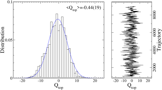
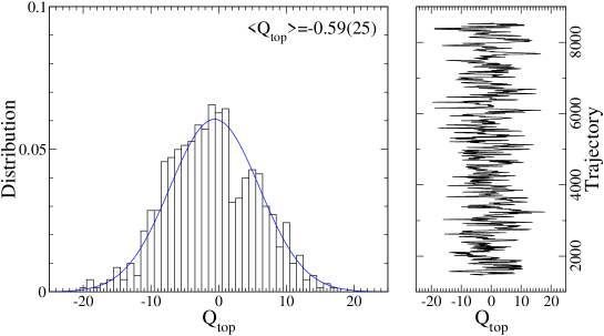
Figure 1: Distribution of topological charge and its Monte Carlo time history. Pion mass 330 MeV (top) and 420 MeV (bottom), Iwasaki 24³, ensembles. The solid line represents a Gaussian distribution function.

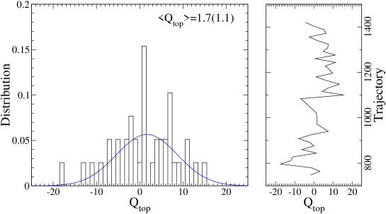
Figure 2: Same as Figure 1 but for the I-DSDR $32^{3}$ ensemble in 170 MeV pion.

The topological susceptibility obtained on these ensembles is

$$\chi_{Q}=\langle Q^{2}\rangle/V = \left\{\begin{array}[]{cl}3.1(2)\times 10^{-4}\textrm{ GeV}^{4}&(\textrm{330 MeV pion, Iwasaki 24${}^{3}$)},\\ 4.4(2)\times 10^{-4}\textrm{ GeV}^{4}&(\textrm{420 MeV pion, Iwasaki 24${}^{3}$)},\\ 0.9(2)\times 10^{-4}\textrm{ GeV}^{4}&(\textrm{170 MeV pion, I-DSDR 32${}^{3}$)},\\ \end{array}\right.$$ (16)

and one sees the suppression with quark mass expected from chiral perturbation theory Leutwyler and Smilga (1992). $\chi_{Q}$ can be used to investigate the relationship between the axial anomaly in QCD and CP-odd effects at $\theta$-NLO Leutwyler and Smilga (1992); Aoki et al. (2007), for instance the mixing angle $\alpha_{N}$ or the nucleon EDM. We discuss this point later.

III.3 Nucleon two-point function

The values of the nucleon mass (energy) and mixing angle $\alpha_{N}$ are obtained by fitting with nucleon two-point function using a single exponential function (see Tab. 2). The nucleon energy and wave function renormalization $Z_{L/G}$ are obtained from the CP-even part of the nucleon propagator ($\theta$-LO) using the spin-projector $P^{+}_{4}$. $\alpha_{N}$ is obtained from the CP-odd part using Eq.(7). Since we are only working to $\theta$-NLO, to reduce the statistical error on $\alpha_{N}$, the mass in the CP-odd part is fixed to the $\theta$-LO mass obtained from the CP-even part. The fit ranges are given Tab. 2, and were chosen to produce a $\chi^{2}/$d.o.f roughly equal to 1, but with as small errors as possible.

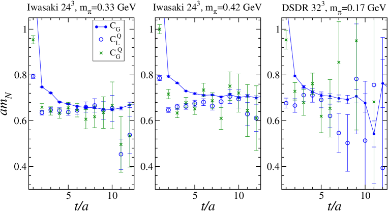
Figure 3: Effective mass of the nucleon ($\theta$-LO, Gaussian smeared sink) compared to the $\theta$-NLO effective mass using local and Gaussian sinks. $m_{\pi}=330$ MeV (left) and 420 MeV (middle), Iwasaki 24³, and 170 MeV, I-DSDR 32³ (right).

As shown in Fig. 3, the effective mass of the $\theta$-NLO nucleon propagator has a clear plateau, and its value is consistent with that from the $\theta$-LO nucleon propagator for both local and smeared sinks. Plateau of effective mass plot for $\theta$-NLO seems to start at shorter time separation than those for $\theta$-LO. We also note the constancy of $\alpha_{N}$ even when the nucleon carries finite momentum which is in agreement with the formulation in Eq.(7). In the following analysis we use $\alpha_{N}$ computed with the Gaussian sink, evaluated at zero momentum.

Table 2: The nucleon energy and its CP-odd mixing angle $\alpha_{N}$. The nucleon energy and $\alpha_{N}$ are given for the Gaussian smeared sink operator.

Iwasaki 243 in 0.33 GeV pion
fit-range	$[6,12]$	$[5,9]$
$\vec{p}^{2}$(GeV2)	$E_{N}$(GeV)	$\alpha_{N}$
0.000	1.1738(25)	-0.356(22)
0.218	1.2618(27)	-0.350(22)
0.437	1.3480(34)	-0.348(22)
0.655	1.4321(52)	-0.342(24)
0.873	1.5092(90)	-0.334(27)
Iwasaki 243 in 0.42 GeV pion
fit-range	$[7,13]$	$[5,9]$
$\vec{p}^{2}$(GeV2)	$E_{N}$(GeV)	$\alpha_{N}$
0.000	1.2641(28)	-0.370(22)
0.218	1.3454(31)	-0.367(23)
0.437	1.4210(40)	-0.366(23)
0.655	1.4931(57)	-0.363(24)
0.873	1.5660(93)	-0.357(27)
I-DSDR 323 in 0.17 GeV pion
fit-range	$[5,10]$	$[5,9]$
$\vec{p}^{2}$(GeV2)	$E_{N}$(GeV)	$\alpha_{N}$
0.000	0.9746(66)	-0.333(128)
0.073	1.0122(69)	-0.269(132)
0.147	1.0491(78)	-0.409(230)
0.220	1.0827(86)	-0.448(287)
0.293	1.1116(114)	-0.381(148)

III.4 Electromagnetic form factor

First we present the CP-even form factors $G_{e}$ and $G_{m}$ obtained from Eq.(10) and Eqs.(8),(9). For the Iwasaki $24^{3}$ ensembles, precise results for the (iso-vector) form factors, using multiple sources method, have appeared previously Yamazaki et al. (2009). Using AMA, we achieve a further reduction of the statistical errors compared to previous work. The precise measurement of the EM form factors is important for the EDM calculation since linear combinations of $G_{e}$ and $G_{m}$ are needed for the subtraction terms proportional to $\alpha_{N}$.

In Figs. 4 and 5 we show the time-slice dependence of the EM form factors for each momenta and also compare the results for two different time-separations, $t_{\rm sep}$, between the nucleon source and sink operators. Suitable nucleon ground state form factors can be extracted from the plateau regions $4\leq t/a\leq 8$, as seen in Fig. 4 (left panel) and $3\leq t/a\leq 6$ in Fig. 5 for the smaller quark mass I-DSDR ensemble (note the electric form factor for the neutron is very small, and should be zero at $q^{2}=0$). In these regions excited state contributions are evidently suppressed. Although increasing $t_{\rm sep}$ reduces excited state contamination, the signal-to-noise ratio also decreases exponentially.

To see whether our value of $t_{\rm sep}$ is large enough, we compare the form factors computed using two different values on the $24^{3}$ ensembles. In the right panel of Fig. 4 one observes a clear plateau between $3\leq t/a\leq 5$ for the smaller value of $t_{\rm sep}$ which is in good agreement with the results shown in the left panel. In Figs. 6 the average values of the form factors are shown. As expected, in Fig. 6 the values for different $t_{\rm sep}$ agree within statistical errors, so we conclude that excited state contamination is small for $t_{\rm sep}\approx 1.3-1.4$ fm source-sink separations used for the observables in this study. A few percent precision on the form factors for $G_{e}^{p}$, $G_{m}^{p}$ and $G_{m}^{n}$ is obtained, and less than 20% precision for $G_{e}^{n}$. For $t_{\rm sep}=0.9$ fm even higher precision is seen despite having only a quarter of the statistics. This indicates that $t_{\rm sep}=0.9$ fm allows good statistical precision while keeping control of excited state contamination.

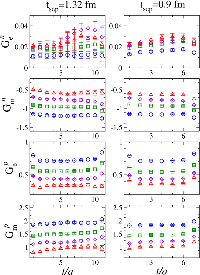
Figure 4: The operator time-slice dependence of electric and magnetic Sachs form factors for the proton and neutron with $t_{\rm sep}=1.32$ fm (left) and $t_{\rm sep}=0.9$ fm (right) in Iwasaki 24³, 330 MeV pion ensemble. Source and sink operators are located in $t/a=0$ and 12 ($t_{\rm sep}=1.32$ fm), and $t/a=0$ and 8 ($t_{\rm sep}=0.9$ fm). Circle, square, diamond and upper-triangle are results at $n_{\vec{p}}^{2}=1$, 2, 3, 4.

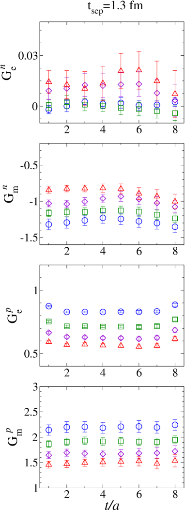
Figure 5: Same as Figure 4 but for I-DSDR 32³, 170 MeV pion ensemble. Source and sink operators are located in $t/a=0$ and 10.

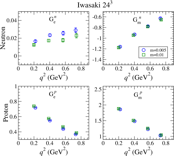
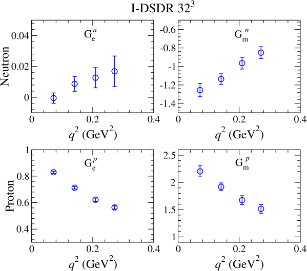
Figure 6: Electric and magnetic form factors. (Top) $m_{\pi}=330$ MeV (circle) and 420 MeV (square), $t_{\rm sep}=0.9$ fm, Iwasaki 24³ ensembles. (Bottom) I-DSDR 32³, 170 MeV pion ensemble.

III.5 EDM form factor

The EDM form factor is extracted from the CP-odd functions given in Eq. (12) which contains $F_{3}$ and terms proportional to $\alpha$ to be subtracted. First we show decomposed $F_{3}$ into two pieces,

$$F_{3}=F_{Q}+F_{\alpha},$$ (17)

with

$$F_{Q} = \frac{m_{N}}{E_{N}+m_{N}}i\frac{2E_{N}}{p_{z}}{\rm tr}\Big{[}P_{5z}^{+}\mathcal{R}^{Q}_{t}\Big{]},$$ (18)

$$F_{\alpha} = \frac{m_{N}}{E_{N}+m_{N}}\alpha_{N}\Big{(}F_{1}+\frac{3m_{N}+E_{N}}{2m_{N}}F_{2}\Big{)},$$ (19)

where $F_{Q}$ contains the total $\theta$-NLO three-point function, and $F_{\alpha}$ contains the subtraction terms. From Figure 7, one sees that $F_{\alpha}$ is relatively precise with a statistical error of about 10%, while that of $F_{Q}$ is more than 50%. This indicates that the ultimate signal-to-noise of $F_{3}$ depends mainly on $F_{Q}$. Again, the region $4\leq t/a\leq 8$ is used to obtain the EDM form factor.

To investigate the presence of excited state contamination, we show the EDM form factor with $t_{\rm sep}=1.32$ fm and $t_{\rm sep}=0.9$ fm in Fig. 8. The smaller separation result has an even better signal than $t_{\rm sep}=1.32$ fm, and their plateaus are consistent. Therefore one sees that the contamination of excited states is negligible in this range.

In Fig. 9 we investigate statistical error scaling by examining subsets of our data and reduced $N_{G}$, the number of source locations of $\mathcal{O}_{G}^{(\rm appx)}$ in the AMA procedure. We find good agreement with the full results, and the statistical error roughly scales with the square root of the number of configurations. Furthermore comparing the full statistics with reduced $N_{G}$, there is a similar reduction of the statistical errors, e.g. the second line in Figure 9 indicates the rate of $52$% with one-quarter statistics (200 configurations) is close to the ideal rate, 50%. In the fourth line, the rate 44% is slightly larger than the ideal rate $1/\sqrt{8}\simeq 35$%. It turns out that the gauge configurations we used do not show strong correlations between different trajectories, and also for AMA there is not a large correlation between different source locations. Our choice of approximation and $N_{G}$ seem to perform well for the statistical error reduction of the EDM form factor for the Iwasaki $24^{3}$ ensembles, and also we find that for the I-DSDR $32^{3}$ ensemble.

In Table 3 and 4, we present the results of the EM and EDM form factors, extracted by fitting the plateaus to a constant value. The EDM form factors for the Iwasaki $24^{3}$ ensembles have roughly 25-30% statistical errors, at best, and the errors grow to more than 100% at worst, depending on the nucleon and momenta. For the I-DSDR 32³ lattice the EDM form factor is very noisy, and we do not observe a clear signal. This is likely due to the relatively poor sampling of the topological charge on this small ensemble of configurations since we do observe relatively small errors for the CP-even EM form factors.

In the next section we estimate the nucleon EDM’s by extrapolating these results to zero momentum transfer.

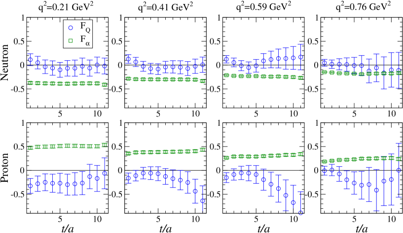
Figure 7: The operator time dependence for the components of the EDM form factor, $F_{Q}$ (total) and the subtraction term $F_{\alpha}$. Momentum transfer increases from left to right. Iwasaki 24³, 330 MeV pion ensemble. The three-point function is defined in (12). The source and sink operators are located in $t/a=0$ and 12.

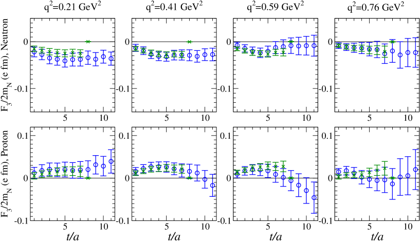
Figure 8: The EDM form factor for different source-sink separations. $t_{\rm sep}=1.32$ fm (circle) and $t_{\rm sep}=0.9$ fm (cross), for neutron (top) and proton (bottom). Iwasaki 24³, 330 MeV pion ensemble, at several momenta indicated in the above of each panel. We locate the source and sink operators in $t/a=0$ and 12 for $t_{\rm sep}=1.32$ fm, $t/a=0$ and 8 for $t_{\rm sep}=0.9$ fm.

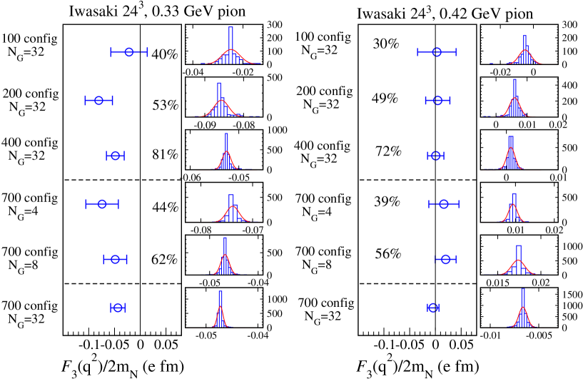
Figure 9: The neutron EDM form factor $F_{3}/2m_{N}$ in e$\cdot$fm unit, the lowest momentum, for various numbers of configurations and values of $N_{G}$. The percentages denote the rates of reduction of statistical errors, defined as the ratio of the statistical error between full (bottom data) and reduced statistics cases. The smaller panels show the distribution of jackknife estimates for each case. The solid line denotes a Gaussian distribution function. 330 MeV pion (left) and 420 MeV pion (right) ensembles.

Table 3: $F^{n}_{3}/2m_{N}$ (e$\cdot$ fm) on Iwasaki 24³ ensemble.

$m=0.005$	P		N
$q^{2}$(GeV2)	$t_{\rm sep}=1.32$ fm	$t_{\rm sep}=0.9$ fm	$t_{\rm sep}=1.32$ fm	$t_{\rm sep}=0.9$ fm
0.210	0.022(17)	0.017( 9)	-0.040(13)	-0.025( 7)
0.405	0.025(12)	0.025( 7)	-0.031( 9)	-0.027( 5)
0.586	0.013(15)	0.028( 7)	-0.018(11)	-0.026( 5)
0.760	-0.001(19)	0.010( 7)	-0.018(14)	-0.016( 6)
$m=0.01$	P		N
$q^{2}$(GeV2)	$t_{\rm sep}=1.32$ fm	$t_{\rm sep}=0.9$ fm	$t_{\rm sep}=1.32$ fm	$t_{\rm sep}=0.9$ fm
0.212	0.034(17)	0.027(15)	-0.005(11)	-0.015(10)
0.412	0.023(13)	0.021(11)	-0.011( 8)	-0.012( 7)
0.604	-0.006(15)	0.014(10)	0.003(10)	-0.010( 7)
0.782	0.012(17)	0.003( 9)	-0.005(12)	-0.002( 7)

Table 4: $F^{n}_{3}/2m_{N}$ (e$\cdot$ fm) on I-DSDR, 32³, 170 MeV pion ensemble.

	P	N
$q^{2}$(GeV2)	$t_{\rm sep}=1.3$ fm	$t_{\rm sep}=1.3$ fm
0.072	0.033(80)	-0.083(34)
0.141	0.057(50)	-0.048(31)
0.208	0.027(69)	-0.028(38)
0.273	-0.057(75)	-0.067(50)

III.6 Lattice results for the neutron and proton EDM

To extrapolate to $q^{2}=0$ a simple linear function consistent with chiral perturbation theory is used,

$$F_{3}(q^{2})/2m_{N}=d_{N}+S^{\prime}q^{2}+\mathcal{O}(q^{4}),$$ (20)

where $d_{N}$ represents the leading order, and $S^{\prime}$ the next-to-leading order in the $q^{2}$ dependence of the EDM form factor. $d_{N}$ is defined as the EDM. Furthermore, according to ChPT Kuckei et al. (2007); Mereghetti et al. (2011) at NLO, $S^{\prime}$ in isoscalar (also isovector) is related to the low-energy constant of CP violating pion-nucleon coupling, and this point is discussed later.

In Figs. 10, we show the $q^{2}$ dependence of the EDM form factors. $F_{3}(q^{2})$ exhibits mild $q^{2}$ dependence within relatively large statistical errors. Since we assume the linear function at low $q^{2}$ region for $F_{3}(q^{2})$, fit ranges in low $q^{2}$, 0.20 GeV${}^{2}<q^{2}<$ 0.6 GeV² in Iwasaki 24³, and 0.07 GeV${}^{2}<q^{2}<$ 0.273 GeV² in DSDR 32³ are chosen. The central values and statistical errors for those fitting are given in Tab. 5, and those lines and error bands are shown in Figure 10. One sees that using such fitting range, we have small $\chi^{2}$/dof, although the extrapolated EDM value has error of about 40–80%, and also the slope of this function, which corresponds to $S^{\prime}$, has almost 100% statistical error. For the near physical pion mass ensemble the relative statistical error is still large: the proton EDM is zero within one standard deviation and the neutron EDM is only non-zero by a bit more than two. Clearly more precision is needed.

Figure 11 displays our results for the EDM as a function of the pion mass squared, and for comparison we show older calculations with $N_{f}=2$ Wilson-clover and Domain-Wall fermions, and recent $N_{f}=3$ Wilson-clover fermions Guo et al. (2015) and $N_{f}=2+1+1$ twisted-mass (TM) fermion Alexandrou et al. (2015). One also sees that our results are comparable with the recent imaginary-$\theta$ calculationGuo et al. (2015) and ETMC collaboration Alexandrou et al. (2015). We note that DWF chiral symmetry forbids potentially large lattice artifacts arising from mixing with chiral broken term associated with Wilson fermions Aoki et al. (1990), unlike the Wilson-clover simulations in Guo et al. (2015) (This corresponds to mixing term with topological charge and pseudoscalar mass term induced by lattice artifact. Since in our case there is small residual mass which controls chiral symmetry breaking, then it is irrelevant in the current precision. However, if considering introducing the higher dimensional CP-violation operator, e.g. chromo-electric dipole moment, the mixing with lower-dimensional operator ($\theta$-term) should be taken into account, see Bhattacharya et al. (2015a) for more details.). Effective theories like chiral perturbation theory Crewther et al. (1979); Mereghetti et al. (2011); Guo and Meissner (2012) and several models in QCD sum rules Pospelov and Ritz (2000); Hisano et al. (2012) have found $d_{N}^{p(n)}=(-)(1$–$4)\times 10^{-3}$ e$\cdot$fm (the minus sign is for the neutron), about one order of magnitude smaller than the central value of lattice QCD results computed at unphysically large pion mass.

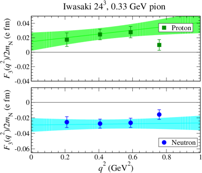
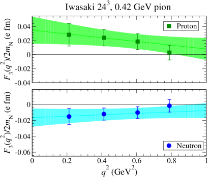
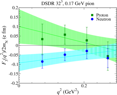
Figure 10: The EDM form factor for neutron (circle) and proton (square), 330 MeV (top) and 420 MeV (middle) pion, Iwasaki $24^{3}$ ensembles, and 0.170 GeV pion (bottom), I-DSDR $32^{3}$ ensemble. In Iwasaki 24³, $t_{\rm sep}=0.9$ fm is used. The lines and bands denote the fitting function with statistical error.

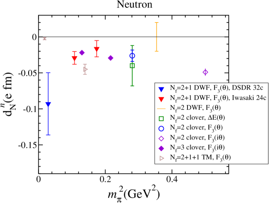
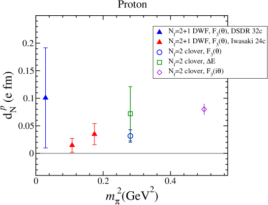
Figure 11: EDM summary plot for the neutron (top) and proton (bottom) for 2 and 3 flavor QCD. Triangles denote results of the current study and include statistical and systematic errors, as described in the text. Results for other methods are also shown: external electric field ($\Delta E$) Shintani et al. (2012), and imaginary $\theta$ ($F_{3}(i\theta)$)Horsley et al. (2008); Guo et al. (2015). Previous results show statistical errors only. Right-triangle is result in $N_{f}=2+1+1$ TM fermion Alexandrou et al. (2015) which is including systematic error. The cross symbol in top panel denotes a range of values from model calculations of neutron EDM based on the baryon chiral perturbation theory Crewther et al. (1979); Mereghetti et al. (2011); Guo and Meissner (2012).

Table 5: Result of EDM which is obtained by the extrapolation of $q^{2}$ to zero with linear ansatz using fitting range of 0.21 GeV² $\leq q^{2}\leq 0.586$ GeV² for 24³ m=0.005, 0.212 GeV${}^{2}\leq q^{2}\leq 0.604$ GeV² for 24³ m=0.01 and 0.072 GeV${}^{2}\leq q^{2}\leq$ 0.273 GeV² for 32³ DSDR m=0.001. The value of $S^{\prime}$ and its $\chi^{2}$/dof are also shown in this table. Here those errors denote statistical one.

Iwasaki 243		Proton			Neutron
$m_{\pi}$ (GeV)	$t_{\rm sep}$ (fm)	$d_{N}^{p}$ (e$\cdot$fm)	$S^{\prime}_{p}$ (e$\cdot$fm3)	$\chi^{2}$/dof	$d_{N}^{n}$ (e$\cdot$fm)	$S^{\prime}_{n}$ (e$\cdot$fm3)	$\chi^{2}$/dof
0.33	1.32	0.030(25)	$-$11.0(21.2)$\times 10^{-4}$	0.7(1.7)	$-$0.053(18)	24.3(14.6)$\times 10^{-4}$	0.2(9)
0.33	0.9	0.015(12)	10.3(8.5)$\times 10^{-4}$	0.1(6)	$-$0.029(8)	1.0(5.4)$\times 10^{-4}$	1.0(2.0)
0.42	1.32	0.064(27)	$-$45.2(21.8)$\times 10^{-4}$	1.3(2.3)	$-$0.021(15)	11.7(12.9)$\times 10^{-4}$	1.8(2.7)
0.42	0.9	0.035(19)	$-$10.4(10.7)$\times 10^{-4}$	0.03(46)	$-$0.016(11)	3.4(5.9)$\times 10^{-4}$	0.02(36)
I-DSDR 323		Proton			Neutron
$m_{\pi}$ (GeV)	$t_{\rm sep}$ (fm)	$d_{N}^{p}$ (e$\cdot$fm)	$S^{\prime}_{p}$ (e$\cdot$fm3)	$\chi^{2}$/dof	$d_{N}^{n}$ (e$\cdot$fm)	$S^{\prime}_{n}$ (e$\cdot$fm3)	$\chi^{2}$/dof
0.17	1.3	0.101(90)	$-$166.4(147.1)$\times 10^{-4}$	0.4(7)	$-$0.093(43)	87.4(74.0)$\times 10^{-4}$	0.5(9)

IV Discussion

The neutron and proton EDM’s induced by the $\theta$-term in the QCD action must vanish in the chiral limit since it can be moved entirely into a pseudoscalar mass term by a chiral rotation because of the QCD axial anomaly  Crewther et al. (1979); Abada et al. (1991a); Aoki and Hatsuda (1992); Cheng (1991); Abada et al. (1991b); Pich and de Rafael (1991); Borasoy (2000); O’Connell and Savage (2006); Kuckei et al. (2007); Ottnad et al. (2010); Mereghetti et al. (2011); Guo and Meissner (2012). Such a mass term vanishes if any of the quarks in the theory are massless. In chiral perturbation theory, the leading behavior Crewther et al. (1979) is

$$d_{N}\approx\frac{\bar{g}_{\pi NN}g_{\pi NN}}{m_{N}}\log\frac{m_{\pi}^{2}}{m_{N}^{2}}$$ (21)

with CP-preserving and CP-violating $\pi$NN coupling, $g_{\pi NN}$ and $\bar{g}_{\pi NN}$ respectively, whereas in the low energy nuclear effective theory Aoki and Hatsuda (1992); Cheng (1991), the EDM can also be described as

$$d_{N}\approx\frac{2}{f_{\pi}^{2}}\chi_{Q}^{2}\mu_{N}\frac{\bar{g}_{\pi NN}}{2m_{N}}$$ (22)

where $\mu_{N}$ is the nucleon magnetic moment, $\chi_{Q}$ is the topological charge susceptibility, which is represented in the leading order in chiral perturbation theory as $\chi_{Q}=m_{\pi}^{2}f_{\pi}^{2}(m_{\eta^{\prime}}^{2}-m_{\pi}^{2})/(N_{f}m_{\eta^{\prime}}^{2})$ Leutwyler and Smilga (1992) (here $f_{\pi}=0.092$ GeV). As given in Eq. (22), topological charge distribution and its susceptibility is related to the EDM, and thus it is interesting to see the relationship between $\chi_{Q}$ and EDM obtained in lattice QCD for the consistency test with effective model. Figure 12 shows such a relationship at our lattice point, and also displays the predicted bound from baryon ChPT at the physical point, for which we use $m_{\pi}=0.135$ GeV and $m_{\eta^{\prime}}=0.957$ GeV. One also sees that for the neutron EDM there is a slight tension between the lattice result and the ChPT estimate, however our simulation point is still far from the physical point.

Although the statistical uncertainty of our lattice results (Fig. 11) is too large to discriminate the quark mass dependence given in (21) or (22), the sign of neutron and proton EDM’s are opposite, and that sign is consistent with the nucleon magnetic moment as one can see in Fig. 4. Further, since the ratio of the proton and neutron EDM’s is given from ratio of those magnetic moments as one can see in Eq. (22), using quark model, its ratio is $(d_{N}^{n}/d_{N}^{p})_{\rm quark}=-2/3$, assuming no SU(2) isospin breaking. Our lattice calculation gives roughly $d_{N}^{n}/d_{N}^{p}\simeq-2$ and $d_{N}^{n}/d_{N}^{p}\simeq-0.5$ for the lighter and heavier $24^{3}$ quark mass ensembles, respectively, the same sign and order of magnitude as the quark model prediction. Note that the analytic result of neutron EDM in NLO SU(2) Kuckei et al. (2007) and SU(3) Ottnad et al. (2010) ChPT suggests that higher order corrections are about 40%, and furthermore there is the additional uncertainty of the CPV $\pi NN$ coupling Bsaisou et al. (2015a, b); Mereghetti and van Kolck (2015).

Nuclei or diamagnetic atoms ($e.g.$, ¹⁹⁹Hg, ¹²⁹Xe) are important experimental avenues for detecting EDM’s. To estimate their EDM’s using an effective theory framework, non-perturbative evaluation of the low energy constants of the theory is essential. The low energy constants related to the quark mass and $q^{2}$ dependence of $F_{3}(q^{2})$ and $S^{\prime}$, for instance, can be obtained from lattice QCD. The values of $S^{\prime}$ in Tab. 5 (statistical errors only) are similar order with the result of SU(3) ChPT at the leading-order, $S^{\prime}_{n}({\rm ChPT})=-3.1\times 10^{-4}$ e$\cdot$fm³ Kuckei et al. (2007) (see also Engel et al. (2013)). Furthermore, according to the argument of NLO BChPT (for details, see Mereghetti and van Kolck (2015)), $S^{\prime}$ for the isoscalar and isovector EDMs, is approximately

$$S^{\prime}_{\rm isoscalar}\simeq 0,\quad S^{\prime}_{\rm isovector}\simeq\frac{g_{A}\bar{g}_{\pi}^{(0)}}{24\pi^{2}f_{\pi}m_{\pi}^{2}}\Big{[}1-\frac{5\pi}{4}\frac{m_{\pi}}{m_{N}}\Big{]},$$ (23)

so $\bar{g}_{\pi}^{(0)}$, the CPV $NN\pi$ coupling, is leading in $S^{\prime}_{\rm isovector}$. Although the precision shown in Tab. 5 is not enough to address this comparison, our results provide a rough bound, $|\bar{g}_{\pi}^{(0)}|\sim O(10^{-1})$. The phenomenological value is also estimated as $\bar{g}_{\pi}^{(0)}\sim 0.04$ Engel et al. (2013).

Finally we consider the chiral behavior of the CP-odd mixing angle $\alpha_{N}$. It depends on the (sea) quark mass but is independent of momentum. Since $\alpha_{N}(\theta)\propto\theta$, it is expected to vanish in the chiral limit. However, as seen in Fig. 13, we observe no significant mass dependence for $\alpha_{N}$ among all of the ensembles in our study. This may simply reflect that the simulations are far from the chiral limit for EDM’s. We also note that the statistical errors are large, especially for the 170 MeV pion ensemble, and there the topological charge distribution is suspect since we have only used 39 configurations.

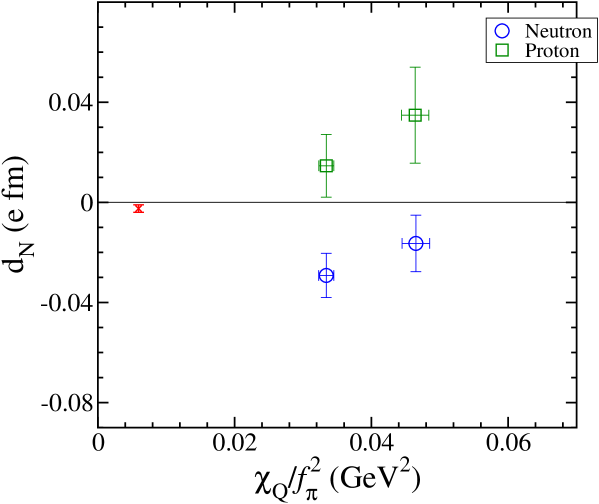
Figure 12: The relation between the nucleon EDM’s and the topological charge susceptibility given in (21) for the neutron (circle) and proton (square) in Iwasaki $24^{3}$ ensembles. The cross symbol is value of neutron EDM from baryon chiral perturbation theory Crewther et al. (1979); Mereghetti et al. (2011); Guo and Meissner (2012).

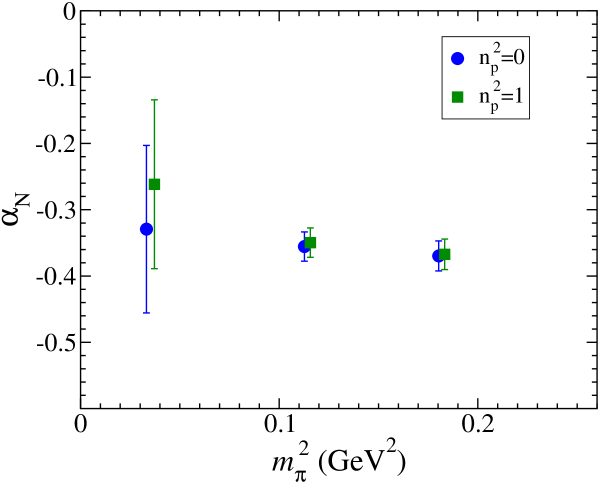
Figure 13: The dependence of pion mass squared for $\alpha_{N}$ obtained by CP-odd nucleon two-point function using the different momenta.

V An exploratory reweighting with topological charge density

Large statistical noise of CP-odd correlation function is possibly due to reweighting with the global topological charge since for many, perhaps most, of the current insertions, there is no overlap with a CP-odd vacuum fluctuation, so reweighting just adds noise to the expectation value. Unfortunately for this study, we have averaged over space on each time slice, so we can not examine these local correlations directly. But we can reweight the correlation function with the charge density summed over a time slice, or several successive time slices. To investigate the above, we sum the topological charge density over a range of time slices, 1, 4, 8 (which is corresponding to temporal location of sink operator) and 64 (which is the maximum size of temporal extension), symmetrically straddling the EM current insertion on a given time slice. A plot of the nucleon EDM for such a reweighting is shown in Fig. 14, and the corresponding mixing angle.

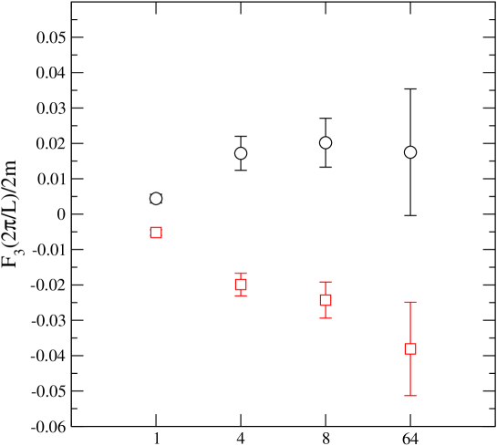
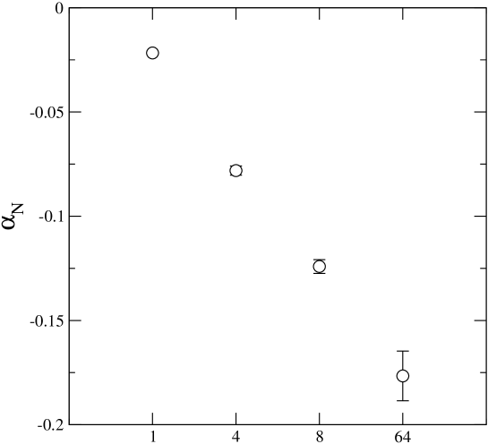
Figure 14: (Top) The nucleon EDM form factors from local time slice reweighting, as described in the text, for the lowest non-trivial momentum. Proton (squares) and neutron (circles). The point on the right corresponds to reweighting with the topological charge $Q$. $24^{3}$, 330 MeV pion ensemble. (Bottom) CP-odd mixing angle from local time slice reweighting, as described in the text, on the same ensemble.

One observes a dramatic decrease in the noise as the number of time slices that are summed for the topological charge density decreases. Interestingly, the values appear to reach a plateau between 9 and 17 time slices. In the future, we plan to investigate spatially local reweighting. One needs to address issues of renormalization as well.

VI Summary

This paper presents a lattice calculation of the nucleon electric dipole moment obtained from the study of the CP-odd form factors of the nucleon in 2+1 flavor QCD with unphysically heavy up and down quarks (the pion mass in this study ranges from 420 down to 170 MeV). The QCD $\theta$-term is included to the lowest order by reweighting correlation functions with the topological charge. We employ the domain wall fermion discretization of the lattice Dirac operator which allows us to control lattice artifacts due to chiral symmetry breaking which may otherwise lead to significant systematic errors in the chiral regime. We applied the all-mode-averaging (AMA) procedure Blum et al. (2013, 2012) to significantly boost the statistical precision of the correlation functions which resulted in statistically significant values of the neutron and proton EDM’s for the two heavier quark ensembles in our study, and a less significant signal for the lightest, 170 MeV pion ensemble. We have examined the pion mass dependence of the EDM’s, which is obtained by linear extrapolation of low momentum transfer to zero momentum transfer with two different time-slice separation of source and sink operators. In this analysis, the effect of excited state contamination is small compared to the statistical error.

In addition, we have investigated the relationship between the local topological charge on each time slice of the lattice and the CP-odd correlation function. This idea may lead to a significant noise reduction in future calculations by reweighting correlation functions with the local topological charge density. We show promising numerical evidence that the large noise associated with global topological charge fluctuations can be reduced.

In this paper, we have concentrated on a high statistics analysis using unphysical masses, $m_{\pi}=$0.17 GeV – 0.42 GeV, and provide lattice QCD results for the nucleon EDMs and form factors with statistical errors only. Future calculations will address systematic errors, including finite size effects (FSE), poor topological charge sampling, the $q^{2}=0$ extrapolation, and lattice spacing artifacts. Baryon chiral perturbation theory (BChPT) in finite volume, to the next-to-leading order O’Connell and Savage (2006); Guo and Meissner (2012); Akan et al. (2014), suggests the magnitude of FSE for our lattice sizes and pion masses are roughly 10%, or less. However additional effects are possible, for instance, at higher order in BChPT. We note several domain-wall fermion gauge ensembles with different lattice cutoffs, volumes and pion masses below 0.2 GeV are available  Arthur et al. (2013); Blum et al. (2014a) to estimate these systematics. Recent developments in numerical algorithms like AMA make it possible to carry out these calculations with current computational resources, and those studies are under way.