Entanglement and RG in the $O(N)$ vector model

Abstract

We consider the large $N$ interacting vector $O(N)$ model on a sphere in $4-\epsilon$ Euclidean dimensions. The Gaussian theory in the UV is taken to be either conformally or non-conformally coupled. The endpoint of the RG flow corresponds to a conformally coupled scalar field at the Wilson-Fisher fixed point. We take a spherical entangling surface in de Sitter space and compute the entanglement entropy everywhere along the RG trajectory. In $4$ dimensions, a free non-conformal scalar has a universal area term scaling with the logarithm of the UV cutoff. In $4-\epsilon$ dimensions, such a term scales as $1/\epsilon$. For a non-conformal scalar, a $1/\epsilon$ term is present both at the UV fixed point, and its vicinity. For flow between two conformal fixed points, $1/\epsilon$ terms are absent everywhere. Finally, we make contact with replica trick calculations. The conical singularity gives rise to boundary terms residing on the entangling surface, which are usually discarded. Consistency with our results requires they be kept. We argue that, in fact, this conclusion also follows from the work of Metlitski, Fuertes, and Sachdev, which demonstrated that such boundary terms will be generated through quantum corrections.

1 Introduction

An important aspect of quantum field theory is the renormalization group (RG) flow between conformal field theories Zamolodchikov:1986gt ; Cardy:1988cwa ; Komargodski:2011vj ; Komargodski:2011xv . Recent results, such as the proof of the F-theorem by Casini and Heurta Casini:2012ei ; Casini:2004bw , strongly suggest entanglement entropy plays an important role in characterizing such flows. For some recent studies of entanglement and RG, see Myers:2010xs ; Giombi:2014xxa ; Ben-Ami:2014gsa ; Park:2015dia ; Fei:2015oha ; Perlmutter:2015vma ; Casini:2015ffa ; Goykhman:2015sga To date, most explicit field theoretic computations of entanglement entropy have focused on the vicinity of fixed points. It is the purpose of this paper to compute entanglement entropy along an entire RG trajectory. We do this for the interacting vector $O(N)$ model at large $N$ in $4$ and $4-\epsilon$ dimensions.

In Sec. 2 we review the entanglement flow equations and recent results in perturbative calculations of entanglement entropy. We establish the setup of our problem: the Euclidean spacetime is taken to be a sphere, and the entangling surface is the bifrucation surface of the equator (see Fig. 1). The radius $\ell$ of the sphere sets the RG scale. The flow equations for the variation of entanglement entropy with respect to $\ell$ reduce to a one-point function of the trace of the stress-tensor.

In Sec. 3 we introduce the vector $O(N)$ model. Within the $\epsilon$ expansion, the RG flow is from the Gaussian fixed point in the UV to the Wilson-Fisher fixed point in the IR. We work to leading order in $1/N$, so that the dynamics is encoded in the mass gap equation. We take the theory to have arbitrary non-minimal coupling in the UV. We renormalize the theory, solve for the beta functions, and compute the expectation value of the trace of the stress-tensor.

In Sec. 4 we find the entanglement entropy as a function of $\ell$. This follows immediately from the results of the previous sections; the general expression is presented in Sec. 4.4. It is instructive to first directly find the entanglement entropy in various limits, and in Sections 4.3, 4.2, we study the UV and IR limits, respectively. In Sec. 4.1 we warm up with the case of strictly four dimensions; this does not have a UV fixed point, but one may still study the entanglement entropy between two points along the RG trajectory.

In Sec. 5 we discuss the implications of our results for computations on backgrounds with conical deficits. The entanglement flow equations imply entanglement entropy is sensitive to the amount of non-minimal coupling to gravity, even in the flat space limit and with interactions. We show this is consistent with replica-trick calculations, but only if one accounts for the contribution of the conical singularity. In fact, this conclusion is unavoidable: even if one chooses to discard such boundary terms, quantum corrections will generate them Sachdev .

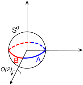
Figure 1: The equator of $S^{d}$ is split into two equal cap-like regions $A$ and $B$ (shown in blue and red respectively). The entanglement entropy is the von Neumann entropy of the density matrix living on the blue region.

2 Review of Entanglement Flow Equations

In this Section we review the entanglement flow equations. The main equation, Eq. 8, expresses the entanglement entropy in terms of the expectation value of the trace of the stress-tensor.

Entanglement entropy is the von Neumann entropy of a reduced density matrix, $\rho$. The entanglement (or modular) Hamiltonian is defined through the reduced density matrix as

$$\rho=e^{-K}~{},\quad\text{Tr}\,\rho=1~{}.$$ (1)

It trivially follows that entanglement entropy is given by the expectation value of the entanglement Hamiltonian,

$$S_{\textrm{\tiny EE}}\equiv-\text{tr}(\rho\log\rho)=\langle K\rangle~{}.$$ (2)

Viewing the expectation value in (2) through the Euclidean path integral representation, the entanglement flow equations Rosenhaus:2014nha ; Rosenhaus:2014woa follow:

$$\frac{\partial S_{\textrm{\tiny EE}}}{\partial\lambda} = -\int\langle\mathcal{O}(x)\,K\rangle\$$ (3)

$$2\frac{\delta S_{\textrm{\tiny EE}}}{\delta g^{\mu\nu}(x)} = -\sqrt{g(x)}\langle T_{\mu\nu}(x)\,K\rangle~{},$$ (4)

where the integral runs over the entire Euclidean manifold parametrized by $x$. These equations describe the change in entanglement entropy under a deformation of the coupling $\lambda$ of some operator $\mathcal{O}$, or under a change in the background metric $g_{\mu\nu}$.

A planar entangling surface in Minkowski space, or a spherical entangling surface in de Sitter space, are especially useful contexts in which to study the flow equations. In these two cases the symmetry in the transverse directions to the entangling surface implies that the entanglement Hamiltonian is proportional to the boost generator (or rotation generator, in the Euclidean continuation) Kabat:1994vj

$$K=\int_{A}T_{\mu\nu}\xi^{\mu}n^{\nu}+c~{},$$ (5)

where $n^{\nu}$ is normal to the entangling surface, $\xi^{\mu}$ is the Killing vector associated with the symmetry, and $c$ is a normalization constant such that $\text{Tr}\,\rho=1$. It should be noted that Eq. 5 is valid for any Lorentz invariant quantum field theory.

Let us review a few properties of the flow equation (3). Since the correlator $\langle T_{ab}\mathcal{O}\rangle$ vanishes for a CFT, the change in entanglement entropy under a deformation away from a fixed point vanishes to first order in $\lambda$ Rosenhaus:2014woa ; Rosenhaus:2014ula . This demonstrates the stationarity of entanglement entropy at the fixed points on a sphere, providing an affirmative answer to the question raised in Klebanov:2012va . The distinction between the conformally and nonconformally coupled scalar is something we will return to. The second order in $\lambda$ part of entanglement entropy is fixed by the correlators $\langle T_{ab}\mathcal{O}\mathcal{O}\rangle$ and $\langle\mathcal{O}\mathcal{O}\rangle$, and is thereby completely universal: the result agrees with both free field and holographic computations Rosenhaus:2014zza . And while these calculations are done for a planar entangling surface, the result for this universal entanglement entropy (log term) is independent of the shape of the entangling surface Rosenhaus:2014zza , as was verified holographically Taylor .

For a planar entangling surface, one can give an independent derivation of (3) Rosenhaus:2014ula . In addition, through use of spectral functions, one can give a compact expression for the entanglement entropy for a general QFT Rosenhaus:2014ula , allowing a demonstration of the equivalence of entanglement entropy and the renormalization of Newton’s constant Casini:2015aa ; Casini:2015ffa .

While a planar entangling surface is a useful and simple case to consider, it is a bit too simple for the study of RG flow of entanglement entropy, as it lacks any scale. A spherical entangling surface is the best suited in this regard, as the size of the sphere sets the RG scale. For an entangling surface that is a sphere in flat space, the entanglement Hamiltonian is only known for a CFT Casini:2011kv , which is sufficient for computing entanglement entropy perturbatively near the fixed point Faulkner:2014jva , but insufficient for finding it along an entire RG trajectory.

In this paper, we study entanglement entropy for a spherical entangling surface in de Sitter space. In this case, one knows the entanglement Hamiltonian along the entire RG trajectory, and the flow equation can be directly applied. The analytic continuation of de Sitter is a sphere $S^{d}$, and the Killing vector $\xi^{\mu}$ is the rotation generator. We will study the change of entanglement entropy as we vary the radius $l$ of $S^{d}$.

Noting that variation of the radius $\ell$ of the space $S^{d}$ can be expressed as,

$$\ell\frac{\partial}{\partial\ell}=-2\int g^{\mu\nu}(x)\frac{\delta}{\delta g_{\mu\nu}(x)}~{},$$ (6)

the flow equation (4) gives,

$$\ell\frac{dS_{\textrm{\tiny EE}}}{d\ell}=\int\langle T_{\mu}^{\mu}(x)\,K\rangle~{}.$$ (7)

As a result of (5), the flow of entanglement entropy can be computed from (7) provided one knows the 2-pt function of the stress-tensor. In fact, a further simplification can be made. As a result of the maximal symmetry of de Sitter space, as well as the Ward identities, the 2-pt function can be reduced to a 1-pt function, turning (7) into Ben-Ami:2015aa

$$\ell\frac{dS_{\textrm{\tiny EE}}}{d\ell}=-{V_{S^{d}}\over d}\,\ell{d\over d\ell}\langle T^{\mu}_{\mu}\rangle~{},$$ (8)

where $V_{S^{d}}$ is the volume of a $d$-dimensional sphere of radius $\ell$. Eq. 8 can also be found directly from the interpretation of entanglement entropy as the thermal entropy in the static patch Ben-Ami:2015aa . The flow equation in the form (8) will be used in Sec. 4 to compute entanglement entropy throughout the RG flow, from $l\rightarrow 0$ in the UV to $l\rightarrow\infty$ in the IR.

3 $O(N)$ on a sphere

In this Section we introduce the field theory background for the $O(N)$ model on a sphere. We work within the $\epsilon$ expansion, so as to have both the free UV and the Wilson-Fisher IR fixed points. We also work at large $N$, allowing us to sum the infinite class of cactus diagrams, as is concisely encoded in the mass gap equation. For the purposes of computing the $\beta$ functions near the fixed points, this is equivalent to working at finite $N$ to one-loop.

After introducing the action and the gap equation in Sec. 3.1, we renormalize the theory and compute the $\beta$ functions in Sec. 3.2, and find the expectation value of the trace of the stress-tensor in Sec. 3.3.

3.1 Gap Equation

The Euclidean action of the $O(N)$ vector model living on a $d$-dimensional sphere of radius $\ell$ is given by,

$$I=\int_{S^{d}}\left[\frac{1}{2}(\partial\vec{\phi})^{2}+{t_{0}\over 2}\vec{\phi}^{2}+{1\over 2}(\xi\eta_{c}+\eta_{0})R\vec{\phi}^{\,2}+\frac{u_{0}}{4N}(\vec{\phi}^{\,2})^{2}\right]+I_{g}~{},$$ (9)

where $R={d(d-1)\over\ell^{2}}$ is the scalar curvature and $\eta_{c}={d-2\over 4(d-1)}$ is the conformal coupling. We take the theory to have arbitrary non-minimal coupling, parameterized by $\xi$; we will be interested in letting $\xi$ have the range $\xi\geq 0$, with $\xi=0$ corresponding to a minimally coupled scalar and $\xi=1$ corresponding to a conformally coupled scalar. The lower bound on $\xi$ follows from the requirement that the theory is stable in the UV.

Since we are on a curved space, we have included $I_{g}$ which describes the purely gravitational counter-terms which must be introduced to cancel the vacuum fluctuations of $\vec{\phi}$,

$$I_{g}=N\int_{S^{d}}\left[\Lambda_{0}+\kappa_{0}R+a_{0}E_{4}+c_{0}R^{2}\right],$$ (10)

where $R$ is the Riemann scalar and $E_{4}=R_{\alpha\beta\gamma\delta}R^{\alpha\beta\gamma\delta}-4R_{\alpha\beta}R^{\alpha\beta}+R^{2}$.

Following the standard large $N$ treatment, we introduce a Lagrange multiplier field $s$ and an auxiliary field $\rho$, so as to write the generating function as

$$Z[\vec{J}]=\int\mathcal{D}s\ \mathcal{D}\rho\ \mathcal{D}\vec{\phi}\ \exp\left(-I-\vec{J}\cdot\vec{\phi}\right)~{},$$ (11)

where the action is

$$I=\int\left[\frac{1}{2}(\partial\vec{\phi})^{2}+{t_{0}\over 2}\vec{\phi}^{2}+{1\over 2}\,\xi\eta_{c}R\ \vec{\phi}^{\,2}+{1\over 2}s(\vec{\phi}^{2}-N\rho)+{N\over 2}\eta_{0}R\rho+N\frac{u_{0}}{4}\rho^{2}\right]+I_{g}~{}.$$ (12)

We can integrate out $\vec{\phi}$ to obtain,

$$Z[\vec{J}]=\int\mathcal{D}s\ \mathcal{D}\rho\ \exp\Big{(}-\frac{N}{2}\int\left(\frac{u_{0}}{2}\rho^{2}-s\rho+\eta_{0}R\rho\right)-\frac{N}{2}\text{Tr}\ln\hat{O}_{s}+\frac{1}{2}\langle\vec{J},\hat{O}^{-1}_{s}\vec{J}\rangle-I_{g}\Big{)}\,,$$ (13)

where $\hat{O}_{s}\equiv-\square+t_{0}+\xi\eta_{c}R+s$ and $\langle,\rangle$ is the $L^{2}$ norm. The contours of integration for the auxiliary fields $s$ and $\rho$ are chosen so as to ensure that the path integral converges.

The auxiliary field $\rho$ has trivial dynamics since it appears algebraically in the action. It can easily be integrated out,

$$Z[{\vec{J}}]=\int\mathcal{D}s\,\exp\Big{(}-\frac{N}{2}\left(\text{Tr}\ln\hat{O}_{s}-\int_{S^{d}}{(s-\eta_{0}R)^{2}\over 2u_{0}}\right)+\frac{1}{2}\langle\vec{J},\hat{O}^{-1}_{s}\vec{J}\rangle-I_{g}\Big{)}\,,$$ (14)

The remaining auxiliary field $s$ encodes the full dynamics of the original $N$ physical degrees of freedom; it is an $O(N)$ singlet, which significantly simplifies the $1/N$ expansion. At large $N$ the theory is dominated by the saddle point, $s(x)=\bar{s}$, which satisfies

$$\bar{s}=u_{0}\langle\phi^{2}\rangle+\eta_{0}R~{},\quad\langle\phi^{2}\rangle\equiv\langle x|\hat{O}_{\bar{s}}^{\,-1}|x\rangle~{}.$$ (15)

It is convenient to re-express (15) in terms of the physical mass, $m^{2}\equiv t_{0}+\bar{s}$,

$$m^{2}=t_{0}+u_{0}\,\langle\phi^{2}\rangle+\eta_{0}R~{}.$$ (16)

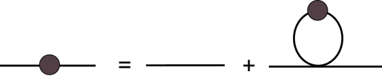
Figure 2: (a) At large $N$ the Schwinger-Dyson equation for the 2-pt function simplifies to become the gap equation (16). (b) Iterating (a) gives a sum of cactus diagrams, such as the one shown above.

Eq. (16) is the gap equation; it has a simple interpretation. At large $N$, fluctuations of $\vec{\phi}^{2}$ are suppressed, $\langle\vec{\phi}^{2}(x)\vec{\phi}^{2}(y)\rangle\approx\langle\vec{\phi}^{2}(x)\rangle\langle\vec{\phi}^{2}(y)\rangle$. The quartic interaction in the action (9) is thus effectively the square of a quadratic, and at leading order in $1/N$ the theory can in some sense be regarded as a free theory with the mass fixed self-consistently through (16). Equivalently, at large $N$ the propagator is found by summing over all cactus diagrams (see Fig. 2); this sum is encoded in (16), as can be seen by iterating (16) starting with the bare mass $t_{0}$.

To solve the gap equation (16) we need the two-point function on a sphere for a free field of mass squared $m^{2}+\xi\eta_{c}R$,

$$\langle\phi_{a}(x)\phi_{c}(y)\rangle=\delta_{ac}\,\frac{l^{2-d}}{(4\pi)^{d/2}}\frac{\Gamma(\lambda)\Gamma(-\lambda+d-1)}{\Gamma(d/2)}\ _{2}F_{1}(\lambda,d-1-\lambda,\frac{d}{2};\cos^{2}\frac{\chi}{2})~{},$$ (17)

where $\chi$ is the angle of separation between $x,y$ and

$$\lambda={d-1\over 2}+i\sqrt{(m\ell)^{2}-{1\over 4}+{d(d-2)(\xi-1)\over 4}}~{}.$$ (18)

In the limit of coincident points (17) becomes

$$\langle\phi^{2}\rangle={\Gamma(1-d/2)\Gamma(\lambda)\Gamma(d-1-\lambda)\over\pi(4\pi)^{d/2}\ell^{d-2}}\sin\big{(}{\pi\over 2}(d-2\lambda)\big{)}\,,$$ (19)

Eq. (19) exhibits a logarithmic divergence in the vicinity of $d=4$, and so we must renormalize the theory.

3.2 Beta functions to leading order in $1/N$

We first consider the counter terms needed to renormalize the couplings $t,u,\eta$ in the action for $\phi$. This is done through use of the gap equation and the requirement of a finite mass $m$.

The divergent piece in the gap equation (16) can be obtained by expanding (19) in $\epsilon\equiv 4-d\ll 1$,

$$\langle\phi^{2}\rangle=\left({(1-\xi)\over 4\pi^{2}\ell^{2}}-{m^{2}\over 8\pi^{2}}\right){m^{-\epsilon}\over\epsilon}+\mathcal{O}(\epsilon^{0})~{}.$$ (20)

To ensure a finite mass gap, $m^{2}$, the bare parameters $u_{0},t_{0}$ and $\eta_{0}$ in Eq. (16) should be renormalized. To find the relation between the bare and renormalized couplings we rewrite Eq. (16) as,

$${m^{2}\over u_{0}}={t_{0}\over u_{0}}+{\eta_{0}\over u_{0}}R-{m^{2}\ell^{\epsilon}\over 8\pi^{2}\epsilon}+{(1-\xi)\ell^{\epsilon}\over 4\pi^{2}\ell^{2}\epsilon}+\ldots~{},$$ (21)

where ellipsis encode finite terms independent of the bare couplings. The absence of poles in the gap equation therefore gives the following relation between the bare and renormalized parameters:

$${1\over u_{0}}={1\over u\mu^{\epsilon}}-{1\over 8\pi^{2}\epsilon\,\mu^{\epsilon}}~{},\quad\quad{t_{0}\over u_{0}}={t\over u\,\mu^{\epsilon}}~{},\quad\quad{\eta_{0}\over u_{0}}={\eta\over u\mu^{\epsilon}}-{1-\xi\over 48\pi^{2}\epsilon\,\mu^{\epsilon}}~{},$$ (22)

where $t,u,\eta$ are the renormalized variables and depend on the RG scale $\mu$.

Applying $\mu{d\over d\mu}$ to both sides of (22), and recalling that the bare couplings are independent of $\mu$, leads to the following set of RG equations:

$$\beta_{u} \equiv \mu{du\over d\mu}=-\epsilon u+{u^{2}\over 8\pi^{2}}={u\over 8\pi^{2}}(u-u^{*})~{},$$

$$\beta_{t} \equiv \mu{dt\over d\mu}={ut\over 8\pi^{2}}~{},$$ (23)

$$\beta_{\eta} \equiv \mu{d\eta\over d\mu}={u\over 8\pi^{2}}\left(\eta-{1-\xi\over 6}\right)~{}.$$

Here $u^{*}=8\pi^{2}\epsilon$ is the well-known Wilson-Fisher IR fixed point, while the Gaussian UV fixed point is at $u=0$.

Our discussion has been general, in that we have allowed the theory to have an arbitrary non-minimal coupling in the UV. Given our conventions for the coefficient of non-minimal coupling to gravity, $(\xi\eta_{c}+\eta_{0})R\vec{\phi}^{2}$ in the action (9), we impose that $\eta=0$ at the UV fixed point. Since the constant $\eta_{c}$ was picked to be $\eta_{c}=1/6$ in $4$ dimesnions, this ensures that for $\xi=1$ the scalar is conformally coupled in the UV, while for $\xi=0$ it is minimally coupled. In fact, (23) tells us that independent of our choice of $\xi$, the IR endpoint of the flow is the same: $\eta^{*}={1-\xi\over 6}$ at the Wilson-Fisher fixed point, and therefore $\xi\eta_{c}+\eta^{*}=1/6$. Thus to leading order in $\epsilon$, a family of weakly interacting, non-conformally coupled massive scalar fields, parametrized by $\xi\geq 0$ in the vicinity of the Gaussian fixed point, all flow to the conformally coupled theory at the Wilson-Fisher fixed point.

3.3 Gravitational counter-terms and energy-momentum tensor

The $\beta$ functions for $u$ and $t$ found in (23) are obviously the same as those in flat space. In addition to $\eta$, the sphere background requires the introduction of gravitational counterterms (10). In this section we compute their $\beta$ functions; the expectation value of the trace of the energy-momentum tensor will then follow. We note that knowing the contribution of the gravitational counterterms is essentially irrelevant for our purposes. We are interested in the area law piece of entanglement entropy, which by necessity involves the mass. The contribution of the gravitational counterterms $aE_{4}$ and $cR^{2}$ only involves the sphere radius $\ell$ and correspondingly will give some constant contribution to the entanglement entropy. The computation of these conterterms is for completeness; the reader uninterested in the details may skip to the result, Eq. (3.3).

Our analysis and notation will closely follow the discussion in Ref. Brown:1980qq . We work on an arbitrary conformally flat curved background, specializing to a sphere at the end. The relation between the bare and renormalized parameters is Brown:1980qq

$$\eta_{0} = (\eta+F_{\eta})Z_{2}^{-1}~{},\quad Z_{2}^{-1}\equiv{t_{0}\over t}~{},$$

$$\Lambda_{0} = \mu^{d-4}(\Lambda+t_{0}^{2}F_{\Lambda})~{},$$

$$\kappa_{0} = \mu^{d-4}(\kappa+2t_{0}\eta_{0}F_{\Lambda}+t_{0}F_{\kappa})~{},$$

$$a_{0} = \mu^{d-4}(a+F_{a})~{},$$

$$c_{0} = \mu^{d-4}(c+\eta_{0}^{2}F_{\Lambda}+\eta_{0}F_{\kappa}+F_{c})~{},$$ (24)

where all counter terms, $Z_{2}^{-1},F_{\eta},F_{\Lambda},F_{\kappa},F_{a}$ and $F_{c}$, are dimensionless functions of the renormalized coupling $u$, and we choose a scheme where they contain only an ascending series of poles in $\epsilon=4-d$. As argued in Brown:1980qq , these functions are independent of the renormalized coupling $\eta$. Furthermore, from (22) we immediately find,

$$Z_{2}^{-1} = \left(1-{u\over 8\pi^{2}\epsilon}\right)^{-1}~{},$$

$$F_{\eta} = {(\xi-1)u\over 48\pi^{2}\epsilon}~{}.$$ (25)

To calculate $F_{\Lambda}$ and $F_{\kappa}$, one can use the definition of the renormalized operator $[\vec{\phi}^{\,2}]$ Brown:1980qq :

$$t[\vec{\phi}^{\,2}]=t_{0}\vec{\phi}^{\,2}+N\mu^{-\epsilon}t_{0}\Big{(}4(t_{0}+\eta_{0}R)F_{\Lambda}+2RF_{\kappa}\Big{)}~{},$$ (26)

and require that its vev is finite. The result is,

$$F_{\Lambda} = {1\over 2(4\pi)^{2}\epsilon}\left(1-{u\over 8\pi^{2}\epsilon}\right)~{},$$

$$F_{\kappa} = {\xi-1\over 96\pi^{2}\epsilon}\left(1-{u\over 8\pi^{2}\epsilon}\right)~{}.$$ (27)

In Appendix A we carry out an independent calculation of $F_{\Lambda}$, finding agreement with Fei:2015oha and the above result. Using these counter terms together with (24), one can evaluate the RG flow equations for $\Lambda$ and $\kappa$,

$$\mu{d\Lambda\over d\mu} = \epsilon\Lambda+{t^{2}\over 2(4\pi)^{2}}~{},$$

$$\mu{d\kappa\over d\mu} = \epsilon\kappa+{t\over(4\pi)^{2}}\left(\eta-{1-\xi\over 6}\right)\,~{}.$$ (28)

The RG equation for $\kappa$ can then be solved,

$$\kappa={\eta\over 2u}\,t+\bar{\kappa}\mu^{\epsilon},$$ (29)

where $\eta^{*}=(1-\xi)/6$ and $\bar{\kappa}$ is some constant that will still need to be fixed.

Turning to the $a$ and $c$ coefficients,

$$\beta_{a} \equiv \mu{da\over d\mu}=\epsilon\,a+f_{a}^{(1)}~{},$$

$$\beta_{c} \equiv \mu{dc\over d\mu}=\epsilon\,c+{\eta^{2}\over 2(4\pi)^{2}}+\eta{\xi-1\over 96\pi^{2}}+f_{c}^{(1)}~{},$$ (30)

where $f_{a}^{(1)}$ and $f_{c}^{(1)}$ are the residues of the simple poles in the definitions of $F_{a}$ and $F_{c}$,

$$F_{a} = {f_{a}^{(1)}\over\epsilon}+{f_{a}^{(2)}\over\epsilon^{2}}+\ldots~{},$$

$$F_{c} = {f_{c}^{(1)}\over\epsilon}+{f_{c}^{(2)}\over\epsilon^{2}}+\ldots~{}.$$ (31)

To calculate $F_{a}$ and $F_{c}$ we will require that the energy-momentum tensor has a finite vev.

Energy-momentum tensor

The energy-momentum tensor of the $O(N)$ model is given by $T_{\mu\nu}=T_{\mu\nu}^{\phi}+T_{\mu\nu}^{g}$ where $T_{\mu\nu}^{\phi}$ is the contribution from $\phi$,

$$T_{\mu\nu}^{\phi} \equiv {2\over\sqrt{g}}{\delta I_{g}\over\delta g^{\mu\nu}}=\nabla_{\mu}\vec{\phi}\nabla_{\nu}\vec{\phi}-g_{\mu\nu}\left({1\over 2}(\partial\vec{\phi})^{2}+{1\over 2}t_{0}\vec{\phi}^{\,2}+{1\over 2}\xi\eta_{c}R\,\vec{\phi}^{\,2}+\frac{u_{0}}{4N}(\vec{\phi}^{\,2})^{2}\right)$$

$$\quad\quad\quad\quad+\xi\eta_{c}R_{\mu\nu}\vec{\phi}^{\,2}+\xi\eta_{c}\left(g_{\mu\nu}\nabla^{2}-\nabla_{\mu}\nabla_{\nu}\right)\vec{\phi}^{\,2}~{},$$

and $T_{\mu\nu}^{g}$ is the gravitational contribution, defined through the variation of the action,

$$T_{\mu\nu}={2\over\sqrt{g}}{\delta I_{g}\over\delta g^{\mu\nu}}.$$ (33)

Taking the trace gives

$$T\equiv g^{\mu\nu}T_{\mu\nu}=-t_{0}\vec{\phi}^{\,2}-{d-2\over 2}E_{0}+(d-4){u_{0}\over 4N}(\vec{\phi}^{\,2})^{2}+(d-1)(\xi-1)\eta_{c}\nabla^{2}\vec{\phi}^{\,2}+T^{g}~{},$$ (34)

where $E_{0}$ is the equation of motion operator

$$E_{0}=\vec{\phi}\left(-\nabla^{2}+\xi\eta_{c}R+t_{0}+\frac{u_{0}}{N}(\vec{\phi}^{\,2})\right)\vec{\phi}~{},$$ (35)

and $T^{g}$ is the trace of the gravitational part,

$${1\over N}T^{g}\equiv{1\over N}g^{\mu\nu}T_{\mu\nu}^{g}=-d\Lambda_{0}-(d-2)\kappa_{0}R-(d-4)(a_{0}E_{4}+c_{0}R^{2})~{},$$ (36)

where we dropped a term proportional to $\nabla^{2}R$, since it vanishes on a sphere.

Taking the vev of the energy-momentum trace and using the gap equation (16): $\langle\vec{\phi}^{2}\rangle=N(m^{2}-t_{0}-\eta_{0}R)/u_{0}$, yields

$${1\over N}\langle T\rangle=-\,{t_{0}\over u_{0}}\,(m^{2}-t_{0}-\eta_{0}R)+(d-4)\,{1\over 4u_{0}}\,(m^{2}-t_{0}-\eta_{0}R)^{2}+{1\over N}T^{g}~{}.$$ (37)

By definition, this expression is finite after the bare parameters are expressed in terms of the renormalized parameters. Substituting (22), (24), (25) and (27) into (37), we get after some algebra,

$${\mu^{\epsilon}\over N}\langle T\rangle = {m^{4}\over 2(4\pi)^{2}}\left(1-{u^{*}\over u}\right)+{t\over u}\Big{(}t-m^{2}+{\epsilon\over 2}\Big{(}m^{2}-{t\over 2}\Big{)}\Big{)}-(4-\epsilon)\Lambda$$

$$+ \left((\epsilon-2)\kappa+\Big{(}1-{\epsilon\over 2}\Big{)}{\eta\over u}\,t+\Big{(}\epsilon\,{\eta\over 2u}+{\xi-1\over 96\pi^{2}}\Big{)}m^{2}\right)R$$

$$+ \epsilon(a+F_{a})E_{4}+\epsilon\left(c-{\eta^{2}\over 4u}+F_{c}+\Big{(}{\xi-1\over 96\pi^{2}\epsilon}\Big{)}^{2}u\right)R^{2}+\mathcal{O}(\epsilon^{2})~{}.$$

Imposing that $\langle T\rangle$ be finite leads to the following large-$N$ results:

$$F_{a} = {f_{a}^{(1)}\over\epsilon}~{},$$

$$F_{c} = {f_{c}^{(1)}\over\epsilon}-\Big{(}{\xi-1\over 96\pi^{2}}\Big{)}^{2}{u\over\epsilon^{2}}~{}.$$ (39)

Both $f_{a}^{(1)}$ and $f_{c}^{(1)}$ are not fixed. However, to leading order in $1/N$ they are identical to their free field values, and we get

$$F_{a} = \frac{-1}{360(4\pi)^{2}\epsilon}~{},$$

$$F_{c} = -\Big{(}{\xi-1\over 96\pi^{2}}\Big{)}^{2}{u\over\epsilon^{2}}~{}.$$ (40)

Combining with (29), the final expression for the trace of energy-momentum tensor takes the form

$${\mu^{\epsilon}\over N}\langle T\rangle = {m^{4}\over 2(4\pi)^{2}}\left(1-{u^{*}\over u}\right)+{t\over u}\Big{(}t-m^{2}+{\epsilon\over 2}\Big{(}m^{2}-{t\over 2}\Big{)}\Big{)}-(4-\epsilon)\Lambda$$

$$+ \left((\epsilon-2)\bar{\kappa}\mu^{\epsilon}+\Big{(}\epsilon\,{\eta\over 2u}+{\xi-1\over 96\pi^{2}}\Big{)}m^{2}\right)R$$

$$+ \epsilon\left(a-\frac{1}{360(4\pi)^{2}\epsilon}\right)E_{4}+\epsilon\left(c-{\eta^{2}\over 4u}\right)R^{2}+\mathcal{O}(\epsilon^{2})~{},$$

where recall that $R$ is the curvature of the sphere, the renormalized couplings are evaluated at RG scale $\mu$, the constant $\xi$ parameterizes the non-minimal coupling ($\xi=1$ for conformally coupled), and $m$ is the physical mass found through the gap equation. In the next section, we use (3.3) to calculate entanglement entropy.

4 Entanglement entropy

Having assembled the necessary field theory ingredients in the previous section, we now compute the entanglement entropy. In what follows we account for the leading order in $1/N$ contributions.

The entanglement entropy is found by solving the flow equation (8), which involves the derivative of $\langle T\rangle$ (3.3) with respect to the sphere radius $\ell$. Since the renormalized couplings $t,u,\eta,\kappa$ are independent of $\ell$, we get

$$\ell{dS_{\textrm{\tiny EE}}\over d\ell}=-{2\pi\,N\,A_{\Sigma}\,\mu^{-\epsilon}\over(4-\epsilon)(3-\epsilon)}\ell^{2}\left({m^{2}\over(4\pi)^{2}}\left(1-{u^{*}\over u}\right)\ell{dm^{2}\over d\ell}+{t\over u}\left({\epsilon\over 2}-1\right)\ell{dm^{2}\over d\ell}-2(\epsilon-2)\bar{\kappa}\mu^{\epsilon}R\right)+s_{0}~{},$$ (42)

where $A_{\Sigma}$ is the area of the entangling surface $\Sigma=S^{d-2}$, $s_{0}$ collectively denotes the contribution of curvature square terms in (3.3), and we used solutions of RG equations for $\kappa$ and $\eta/u$ to simplify the linear curvature term in (3.3), see (29) and (66). We ignore the $s_{0}$ terms as they are $m$-independent, and therefore just give some constant contribution to the entanglement entropy. The solution for entanglement entropy along the RG trajectory follows upon substituting the solutions of the gap equation (16) and the beta functions (23) into (42) and integrating.

There are, however, a few caveats associated with the standard ambiguities of renormalization. Indeed, the couplings in the above expression depend on an arbitrary RG scale, $\mu$, as well as on the choice of renormalization scheme. This ambiguity is unsurprising, and reflects the well-known fact that entanglement entropy in field theory depends on the details of the regularization procedure, and is therefore scheme dependent. However, certain contributions to the entanglement entropy, ‘universal entanglement entropy’, are unaffected by a change in the regularization scheme. It is these terms that we will be interested in calculating.

There are three competing scales: $\mu$, $\ell$, and the asymptotic mass $m_{\infty}$ given through the solution of the gap equation (16) in the limit of flat space.. Since the curvature of the sphere sets the characteristic energy scale, we must have $\mu\sim\ell^{-1}$. The constant of proportionality between $\mu$ and $\ell^{-1}$ is arbitrary, though this is no different than the usual freedom to rescale $\mu$. In our context, this constant of proportionality is exchanged for the entanglement entropy at some radius $\ell$. Or, put differently, we can express the entanglement entropy at radius $\ell_{1}$ in terms of the entanglement entropy at some other radius $\ell_{0}$.

Furthermore, there is a substantial difference between the two cases characterized by $\epsilon=0$ and $\epsilon\neq 0$. In the former case the theory is not UV complete; as $m\ell$ runs from small to large values, it flows from a nonconformal interacting field theory in the UV to a Gaussian IR fixed point. In contrast, for finite $\epsilon\ll 1$, the system flows from the Gaussian UV fixed point at $m_{\infty}\ell\ll\epsilon\ll 1$, into the interacting Wilson-Fisher IR fixed point at $m_{\infty}\ell\gg\epsilon^{-1}\gg 1$. In particular, there is no smooth limit which interpolates between the two cases, and we analyze them separately. We consider $\epsilon=0$ in Sec. 4.1, and finite $\epsilon$ in Sec. 4.2, 4.3, and 4.4. Note that in 4-dimensions, the coefficient of the $\log$ term is universal. In $4-\epsilon$ dimensions there is no $\log$ term, however a $1/\epsilon$ term turns into a $\log$ in the limit of $\epsilon\rightarrow 0$.

4.1 Four dimensions

In this section we compute the entanglement entropy in $4$ dimensions. Taking the limit $\epsilon\to 0$ results in the following RG flow equations,

$$\mu{du\over d\mu} = {u^{2}\over 8\pi^{2}}~{},$$

$$\mu{d\over d\mu}\left({\eta\over u}\right) = {\xi-1\over 48\pi^{2}}~{}.$$ (43)

Integrating gives,

$$u(\mu) = {u_{0}\over 1-{u_{0}\over 8\pi^{2}}\log(\mu\delta)}~{},$$

$${\eta\over u} = {\xi-1\over 48\pi^{2}}\log\left(\mu\delta\right)~{},$$ (44)

where we imposed the initial conditions $(u,\eta)=(u_{0},0)$ at the UV scale $\delta$. In the deep IR (44) gives $(0,(1-\xi)/6)$.

The 4D counterparts of (3.3) and (42) are

$${\langle T\rangle\over N} = {m^{4}\over 2(4\pi)^{2}}+{t\over u}\Big{(}t-m^{2}\Big{)}-4\Lambda-\left(2\bar{\kappa}+{1-\xi\over 96\pi^{2}}\,m^{2}\right)R-\frac{E_{4}}{360(4\pi)^{2}}~{},$$ (45)

and

$$\ell{dS_{\textrm{\tiny EE}}\over d\ell} = {\pi\,N\,A_{\Sigma}\over 6}\ell^{2}\left({t\over u}\,\ell{dm^{2}\over d\ell}-4\bar{\kappa}R\right)+s_{0}~{},$$ (46)

while the gap equation (16) can be succinctly written as

$${t\over u}={m^{2}\over u(m)}-{\xi-1\over 4\pi^{2}\ell^{2}}\log(m\delta)-\langle\phi^{2}\rangle_{\text{reg}}~{},$$ (47)

where we used (44), and the last term denotes the regular part of the 4D two-point function in the limit of coincident points, see (20),

$$\langle\phi^{2}\rangle_{\text{reg}}\equiv\lim_{\epsilon\to 0}\left[\langle x|\left(-\square+m^{2}+\xi\eta_{c}R\right)^{\,-1}|x\rangle-\left({(1-\xi)\over 4\pi^{2}\ell^{2}}-{m^{2}\over 8\pi^{2}}\right){m^{-\epsilon}\over\epsilon}\right]~{}.$$ (48)

Applying a derivative with respect to $\ell$ to both sides of (47), yields

$$\ell{dm^{2}\over d\ell}\left(1+{u(m)\over 8\pi^{2}}\Big{(}{1-\xi\over(m\ell)^{2}}-{1\over 2}\Big{)}\right)=u(m)\,{1-\xi\over 2\pi^{2}\ell^{2}}\log(m\delta)+u(m)\,\ell{d\over d\ell}\langle\phi^{2}\rangle_{\text{reg}}$$ (49)

This expression together with (46) and (47) provides a full solution for entanglement entropy flow on a sphere. Note that the RG scale $\mu$ is completely eliminated from the final answer. Effectively its role is played by the radius of the sphere, $\ell$, as the curvature of the background sets the characteristic energy scale for excitations. In particular, the deep IR and UV are defined by $m\ell\gg 1$ and $m\ell\ll 1$, respectively. Of course, we have assumed that the physical scales $m$ and $\ell$ are far away from the microscopic UV cut off $\delta$,

$$m\delta\ll 1\quad\text{and}\ \quad\ell\gg\delta~{}.$$ (50)

Now we explicitly evaluate EE in the UV and IR regimes. We start from the former. Using (19) to evaluate $\langle\phi^{2}\rangle_{\text{reg}}$ and substituting the result into (49), yields

$$\ell{dm^{2}\over d\ell}\Big{|}_{m\ell\ll 1}=u(m){\xi-1\over 2\pi^{2}\ell^{2}}\big{(}\log(m\ell)-\log(m\delta)+\ldots\big{)}+\mathcal{O}(u(m)^{2})~{},$$ (51)

where ellipsis denote subleading terms in $m\ell\ll 1$. Similarly, from the gap equation (47), we get

$$u(m){t(\mu)\over u(\mu)}\Big{|}_{m\ell\ll 1}=m^{2}+2{\xi-1\over\ell^{2}}\,+\ldots~{}.$$ (52)

Only the first term on the right hand side contributes to the ‘area law’, while other terms are either subleading corrections or contribute to a constant term in the entanglement entropy. Hence,

$$\ell{dS_{\textrm{\tiny EE}}\over d\ell}\Big{|}_{m\ell\ll 1}=N(\xi-1)\,{A_{\Sigma}\,m^{2}\over 12\pi}\log{\ell\over\delta}-8\pi\,N\,A_{\Sigma}\bar{\kappa}+\ldots~{},$$ (53)

Similarly, in the IR regime we have

$$\ell{dS_{\textrm{\tiny EE}}\over d\ell}\Big{|}_{m\ell\gg 1}=N(1-\xi)\,{A_{\Sigma}\,m^{2}\over 12\pi}\log(m\delta)-8\pi\,N\,A_{\Sigma}\bar{\kappa}+\ldots~{}.$$ (54)

The above behavior of entanglement entropy has a simple physical interpretation. In the UV regime we have $1\ll{\ell\over\delta}\ll{1\over m\delta}$, and the universal ‘area law’ of entanglement scales as $\ell^{2}\log(\ell/\delta)$, i.e., there is a logarithmic enhancement relative to the standard growth $\sim\ell^{2}$. This enhancement persists as we increase $\ell$ until $\ell m\sim 1$ is reached. Effectively, the universal ‘area law’ at $m\ell\sim 1$ is built from all the massive degrees of freedom which have almost decoupled at this point. As we continue increasing $\ell$, the universal ‘area law’ continues growing like $\ell^{2}$ until the hierarchy of scales is reversed, $1\ll{1\over m\delta}\ll{\ell\over\delta}$, and the flow terminates at the IR fixed point.

In particular, the logarithmic ‘area law’ in the deep IR represents entanglement of UV degrees of freedom. It has nothing to do with the IR field theory, which is empty in our case. As was noted in Rosenhaus:2014woa ; Rosenhaus:2014ula (see Sec. 2), the universal entanglement entropy vanishes for a conformally coupled scalar. Setting $\xi=1$ in (54) and (53) recovers this result.

4.2 Wilson-Fisher fixed point

In this section we calculate the entanglement entropy at the Wilson-Fisher fixed point in $4-\epsilon$ dimensions. This requires evaluating the right hand side of (42), which involves the derivative of $m^{2}$ with respect to $\ell$.

We start by expanding (19) in $m\ell\gg\epsilon^{-1}\gg 1$,

$$\langle\phi^{2}\rangle={(4\pi)^{\epsilon\over 2}\over(2\pi)^{2}\epsilon(\epsilon-2)}\Gamma\left(1+{\epsilon\over 2}\right)m^{2-\epsilon}\left(1-{(\epsilon-4)(\epsilon-2)(6(1-\xi)+\epsilon(3\xi-2))\over 24\,(m\ell)^{2}}+\mathcal{O}\big{(}(m\ell)^{-4}\big{)}\right)$$ (55)

Now using (16), (22) and (55) results in

$$t^{*}={2(4\pi)^{\epsilon\over 2}\over(2-\epsilon)}\Gamma\left(1+{\epsilon\over 2}\right)m^{2}\left({m\over\mu}\right)^{-\epsilon}\left(1-{(\epsilon-4)(\epsilon-2)(6(1-\xi)+\epsilon(3\xi-2))\over 24\,(m\ell)^{2}}+\mathcal{O}\big{(}(m\ell)^{-4}\big{)}\right)~{},$$ (56)

where the asterisk in $t^{*}$ denotes that the system sits at the Wilson-Fisher fixed point. Differentiating (56) with respect to $\ell$ yields,

$$\ell{dm^{2}\over d\ell}\Big{|}_{m\ell\gg 1}=m^{2}\left(-{(\epsilon+2)(\epsilon-4)(\epsilon-2)(6(1-\xi)+\epsilon(3\xi-2))\over 24\,(m\ell)^{2}}+\mathcal{O}\big{(}(m\ell)^{-4}\big{)}\right)~{},$$ (57)

Substituting this expression and (56) into (42) gives

$$\ell{dS_{\textrm{\tiny EE}}\over d\ell}\Big{|}_{m\ell\gg 1} = {(4\pi)^{{\epsilon\over 2}-1}(\epsilon-2)\big{(}6(1-\xi)+\epsilon(3\xi-2)\big{)}\over 12\,\epsilon\,(3-\epsilon)}\,\Gamma\left(2+{\epsilon\over 2}\right)\,NA_{\Sigma}m^{2-\epsilon}\Big{(}1+\mathcal{O}\big{(}(m\ell)^{-2}\big{)}\Big{)}$$ (58)

$$+ 4\pi(\epsilon-2)\,N\,A_{\Sigma}\bar{\kappa}+s_{0}~{},$$

The first thing to note about (58) is that the ‘area law’ term does not have any $\mu$-dependance, and therefore it is not sensitive to the constant of proportionality in the relation $\mu\sim\ell^{-1}$, i.e., as expected, the value of entanglement entropy at the fixed point is invariant under reparametrizations of the RG trajectory.

It is instructive to compare (58) with its counterpart in Sachdev . The results in Sachdev are intrinsic to the Wilson-Fisher fixed point since their setup, unlike ours, confines the RG flow to the IR end. The geometry in Sachdev is flat, and therefore the gravitational coupling, $\bar{\kappa}$, which appears in (58) is absent. In addition, as we argue in section 5, the computation of Sachdev corresponds to $\xi=1$ at the Wilson-Fisher fixed point. Thus, to leading order in $\epsilon\ll 1$, Eq. (58) reduces to

$$\ell\frac{dS_{\textrm{\tiny EE}}}{d\ell}\Big{|}_{m\ell\gg 1}\simeq-N\,{A_{\Sigma}m_{\textrm{\tiny$\infty$}}^{2-\epsilon}\over 72\pi}\quad\Leftrightarrow\quad S_{\textrm{\tiny EE}}\simeq-N\,{A_{\Sigma}m_{\textrm{\tiny$\infty$}}^{2-\epsilon}\over 144\pi}~{},$$ (59)

where $m_{\textrm{\tiny$\infty$}}$ is the mass gap in the limit of flat space. Eq. (59) is in agreement with Sachdev . A simple derivation of (59) was later given by Casini, Mazzitelli and Testé Casini:2015aa . The authors noticed that to leading order in $\epsilon$, the anomalous dimension vanishes at the Wilson-Fisher fixed point, and thus (59) may be found from the entanglement entropy for a free field. One distinction between our work and that of Casini:2015aa , is that Casini:2015aa advocates that the entanglement Hamiltonian has a discontinuous jump at the UV fixed point. Namely, that the entanglement entropy takes the value for the minimally coupled scalar at the free field endpoint of the RG trajectory, whereas it takes the conformally coupled value at all other locations. In our setup, the entanglement entropy behaves smoothly along the entire RG trajectory. As found from the beta functions (23), starting with either a minimally or nonminimally coupled field in the UV leads to the conformally coupled field in the IR.

Let us now expand the numerical coefficient of the ‘area law’ term in (58) in $\epsilon\ll 1$

$$\ell{dS_{\textrm{\tiny EE}}\over d\ell}\Big{|}_{m\ell\gg 1} = {N\,A_{\Sigma}m^{2-\epsilon}\over 12}\left({-1\over 6\pi}+(\xi-1)\left({1\over\pi\epsilon}-{2\gamma+2/3-2\log(4\pi)\over 4\pi}\right)+\mathcal{O}\big{(}\epsilon,(m\ell)^{-2}\big{)}\right)$$ (60)

$$+ 4\pi(\epsilon-2)\,N\,A_{\Sigma}\bar{\kappa}+s_{0}~{}.$$

In the next section, we will see that the $1/\epsilon$ term in (60) is associated with UV degrees of freedom. The presence of this UV remnant is a result of using the full energy-momentum tensor (3.3) to calculate entanglement entropy at any scale $\mu\sim\ell^{-1}$.

To isolate entanglement entropy intrinsic to the scale $\ell$, one needs to use some kind of subtraction scheme. There is no unique or preferred choice of such a scheme. Renormalized entanglement entropy Liu:2012eea is one possibility. This prescription proved to be particularly powerful in three dimensions, and was used in the proof Casini:2012ei of the F-theorem Jafferis:2011zi , see also Casini:2015woa . Unfortunately, it is not clear that renormalized entanglement entropy has analogous properties, such as monotonicity, in integer dimensions higher than the $3$; nor is it clear how to apply it in non-integer dimensions.

For the particular choice of $\xi=1$, the theory is conformally coupled along the entire RG trajectory, and the contribution of UV degrees of freedom to the ‘area law‘ in the vicinity of $d=4\,(\epsilon=0)$ vanishes. Since in this case (58) is not contaminated by UV physics, it can be used to find an approximation for entanglement entropy at the interacting IR fixed point in three dimensional flat space. Substituting $\xi=\epsilon=1$ and $\bar{\kappa}=0$ into (58), gives

$$S^{\textrm{\tiny IR}}_{\textrm{\tiny EE}}\Big{|}_{d=3} \simeq -{N\over 64}mA_{\Sigma}~{}.$$ (61)

We note that the constant $\bar{\kappa}$ is arbitrary; it can be exchanged for the entanglement entropy at some scale $l_{1}$. A choice that would seem natural is to demand that entanglement entropy vanishes in the deep IR (as a result of the mass gap, all degrees of freedom decouple in the IR, and the Wilson-Fisher fixed point is thus empty). This results in

$$S_{\textrm{\tiny EE}}\Big{|}_{m\ell\gg 1}=0\quad\Rightarrow\quad\bar{\kappa}=m^{2-\epsilon}{(4\pi)^{{\epsilon\over 2}-2}\big{(}6(\xi-1)-\epsilon(3\xi-2)\big{)}\over 12\,\epsilon\,(3-\epsilon)}\,\Gamma\left(2+{\epsilon\over 2}\right)~{}.$$ (62)

The above subtraction scheme is special to a curved manifold with nondynamical gravity, where there is an extra parameter $\bar{\kappa}$. However in flat space $\bar{\kappa}=0$, and one is forced to adopt a different subtraction scheme. Another drawback of the choice (62) is that it modifies entanglement entropy at all points along the RG trajectory, and not only in the deep IR limit. The latter makes it difficult to extrapolate the results for an ‘area law’ on a sphere to flat space which has no analog of $\bar{\kappa}$. In what follows we simply leave $\bar{\kappa}$ unspecified.

4.3 Gaussian fixed point

This time we expand (19) in $m\ell\ll\epsilon\ll 1$. In this regime the theory flows to the Gaussian UV fixed point where $u$ asymptotically vanishes, $u\ll\epsilon$. From the gap equation,

$$\langle\phi^{2}\rangle\Big{|}_{m\ell\ll 1} = \alpha_{1}m^{2}\ell^{\epsilon}\left({1\over(m\ell)^{2}}+\alpha_{2}+\mathcal{O}\left((m\ell)^{2}\right)\right)~{},$$ (63)

where $\lambda_{0}=\lambda|_{m\ell=0}$ and for brevity we introduced the following constants

$$\alpha_{1} \equiv {\Gamma\big{(}{\epsilon-2\over 2}\big{)}\Gamma(\lambda_{0})\Gamma(\bar{\lambda}_{0})\cosh\big{(}{\pi(\lambda_{0}-\bar{\lambda}_{0})\over 4i}\big{)}\over\pi(4\pi)^{4-\epsilon\over 2}}~{},$$

$$\alpha_{2} \equiv 2\,{\psi(\bar{\lambda}_{0})-\psi(\lambda_{0})+i\pi\tanh\big{(}{\pi(\lambda_{0}-\bar{\lambda}_{0})\over 4i}\big{)}\over\lambda_{0}-\bar{\lambda}_{0}}~{},$$ (64)

where $\psi(\lambda)$ is the digamma function. The two terms that we kept in (63) are the only ones that diverge as $\epsilon\to 0$. We now substitute this expansion into (16) and use (22)

$$m^{2}\left({1\over u}-{1\over 8\pi^{2}\epsilon}\right)={t\over u}+\alpha_{1}m^{2}(\mu\ell)^{\epsilon}\left({1\over(m\ell)^{2}}+\alpha_{2}+\mathcal{O}((m\ell)^{2})\right)+\left({\eta\over u}-{1-\xi\over 48\pi^{2}\epsilon}\right)R~{}.$$ (65)

Solving the RG equation for $\eta$ and $u$ gives

$${\eta\over u}={1-\xi\over 48\pi^{2}\epsilon}~{}.$$ (66)

Hence, we can drop the last term in (65),

$$\ell{dm^{2}\over d\ell}\Big{|}_{m\ell\ll 1}=u\,\alpha_{1}m^{2}(\mu\ell)^{\epsilon}\left({\epsilon-2\over(m\ell)^{2}}+\epsilon\,\alpha_{2}+\mathcal{O}\big{(}(m\ell)^{2}\big{)}\right)+\mathcal{O}(u^{2})~{}.$$ (67)

Substituting (65) and (67) into (42), we finally deduce,

$$\ell{dS_{\textrm{\tiny EE}}\over d\ell}\Big{|}_{m\ell\ll 1}=-{2\pi\alpha_{1}(2-\epsilon)\over(4-\epsilon)(3-\epsilon)}\,NA_{\Sigma}m^{2}\ell^{\epsilon}\Big{(}1+\mathcal{O}(u)\Big{)}+4\pi(\epsilon-2)\,N\,A_{\Sigma}\bar{\kappa}+\mathcal{O}\big{(}(m\ell)^{4}\big{)}+s_{0}~{}.$$ (68)

Expanding the coefficient of $A_{\Sigma}m^{2}\ell^{\epsilon}$ in $\epsilon\ll 1$, we get

$$\ell{dS_{\textrm{\tiny EE}}\over d\ell}\Big{|}_{m\ell\ll 1}=N\,A_{\Sigma}m^{2}\ell^{\epsilon}\left({\xi-1\over 12\pi\epsilon}+\mathcal{O}(\epsilon,u)\right)+4\pi(\epsilon-2)\,N\,A_{\Sigma}\bar{\kappa}+\mathcal{O}\big{(}(m\ell)^{4}\big{)}+s_{0}~{}.$$ (69)

As in the previous case, the $\mu$ dependence drops out of the final answer. While we implicitly assumed that $\mu\sim\ell^{-1}$, the final answer for entanglement entropy at the fixed point should not be sensitive to the $\mathcal{O}(1)$ coefficient of proportionality between $\mu$ and $\ell$. Furthermore, the $1/\epsilon$ term is the same term that appears in (58), which, as mentioned in the previous section and now seen explicitly in (69), represents entanglement entropy of the UV degrees of freedom.

For a minimally coupled scalar field, $\xi=0$, and we recover the well-known universal ‘area law’, in agreement with Sachdev and Hertzberg:2010uv ; Huerta:2011qi ; Lewkowycz:2012qr (this is just $N$ times the answer for a free scalar). If, however, the field is non-minimally coupled, we get a different answer which vanishes at the conformal point $\xi=1$. In Sec. 5.3, we show how to generalize the calculation at the Gaussian fixed point presented in Sachdev , so as to take into account the contribution from non-minimal coupling.

4.4 Along the RG trajectory

In this section we write down the entanglement entropy for the $O(N)$ model for a conformally coupled scalar, at leading order in $1/N$ in dimension $4-\epsilon$, for any sphere of radius $\ell$. The ingredients have been worked out in the previous sections; here we just collect them.

Solving the RG equation (23) gives

$$u(\mu)=\frac{u^{*}}{1+\left(\frac{\mu}{\mu_{0}}\right)^{\epsilon}}~{},$$ (70)

where $\mu_{0}$ is an arbitrary constant scale and $u^{*}$ is $u$ at the Wilson-Fisher fixed point. We want to take $\mu=1/\ell$, and we let $\mu_{0}=\ell_{0}^{-1}$. We will write this as

$$u(\ell)=\frac{u^{*}}{1+\left(\frac{\ell_{0}}{\ell}\right)^{\epsilon}}~{}.$$ (71)

Note that the entanglement entropy will contain the constant $\ell_{0}$. This is analogous to how correlation functions contain an arbitrary scale which is calibrated through some measurement. In our context, it means entanglement entropy needs to me measured at one value of $\ell$, and can then be predicted at all other values.

The gap equation is given by

$$m^{2}\left(\frac{1}{u}-{1\over u^{*}}\right)=\frac{t}{u}+\ell^{-\epsilon}\langle\phi^{2}\rangle~{},$$ (72)

where for simplicity we chose $\xi=1$ (hence, $\eta=0$ along the entire RG flow) and $\langle\phi^{2}\rangle$ is given by (19). Also,

$$\ell\frac{d}{d\ell}\big{(}\ell^{-\epsilon}\langle\phi^{2}\rangle\big{)}=\left(\ell\frac{d\lambda}{d\ell}\frac{\partial}{\partial\lambda}-2\right)\big{(}\ell^{-\epsilon}\langle\phi^{2}\rangle\big{)}~{},$$ (73)

where $\lambda$ is a function of $m\ell$ and is given by (18). Differentiating (72) and using (73), we can solve for $\ell\frac{dm^{2}}{d\ell}$.

The entanglement entropy is given by (42), where we substitute $u(\ell)$ given by (71) and $t/u$ given by (72). We thus have a complete expression for entanglement entropy in terms of the mass $m$ and radius $\ell$.

5 Boundary perturbations

In the previous Section we computed entanglement entropy along the entire RG flow, and in particular in the proximity of the fixed points. The entanglement entropy was found to be sensitive to the non-minimal coupling parameter $\xi$. This sensitivity is robust: it persists in the flat space limit, and away from the UV fixed point.

In light of these results, in this Section we revisit the replica-trick calculations of entanglement entropy near fixed points. The fact that entanglement entropy depends on $\xi$, even in flat space, is manifest in the context of the replica-trick, and is a consequence of the curvature associated with the conical singularity. What is unclear is if this boundary term which gives $\xi$ dependance is real, or an artifact of the replica-trick which should be discarded. The results of Sec. 4 suggest the former.

In Sec. 5.1 we review the replica-trick calculation of entanglement entropy for a free scalar field using heat kernel techniques. In Sec. 5.2 we review a calculation of Metlistski, Fuertes, and Sachdev Sachdev which finds that loop corrections generate a boundary term, and we argue that this has a simple interpretation as the classical boundary term of Sec. 5.1 due to the curvature of the conical singularity. In Sec. 5.3 we generalize the calculation of Sachdev of entanglement entropy at the Gaussian fixed point, so as to incorporate non-minimal coupling, and find agreement with the results of Sec. 4.

5.1 Replica trick: Free energy

Here we preform the standard replica trick calculation for a free massive scalar Kabat95 ; Callan:1994py ; SusUgl94 . Recall that entanglement entropy is computed from the variation of the free energy,

$$S=\left(\beta\frac{\partial}{\partial\beta}-1\right)\Big{|}_{\beta=2\pi}(\beta F)~{},$$ (74)

where the effective action $(\beta F)$ is evaluated on a space which is a cone with a deficit angle $2\pi-\beta$. Eq. (74) is just the standard thermodynamic equation for entropy; the need to vary the temperature away from $1/2\pi$ introduces a conical singularity at the origin. The effective action, after integrating out the matter, is expanded in derivatives of the metric,

$$\beta F=-\frac{1}{2}\int_{\mathcal{M}}\int_{\delta^{2}}^{\infty}\frac{ds}{(4\pi s)^{d/2}}e^{-sm^{2}}\left(\frac{c_{0}}{s}+c_{1}R+\mathcal{O}(s)\right)$$ (75)

The relevant term is the one proportional to the scalar curvature, whose integral on a cone is $\int_{\mathcal{M}}R=2\mathcal{A}_{\Sigma}\,(2\pi-\beta)$. Thus the entropy is,

$$S=2\pi\,c_{1}\,\mathcal{A}_{\Sigma}\,\int_{\delta^{2}}^{\infty}\frac{ds}{(4\pi s)^{d/2}}e^{-sm^{2}}~{}.$$ (76)

Specializing to $d=4$ and expanding the exponential in (76) to extract the $\log$ divergent piece, we get,

$$S=\frac{c_{1}}{4\pi}\,m^{2}\,\mathcal{A}_{\Sigma}\,\log(\delta)~{}.$$ (77)

For the minimally coupled scalar $c_{1}=1/6$, while for the conformally coupled scalar $c_{1}=0$ Vas .

This computation is, of course, not new. However, it conflicts with the belief that (in the flat space limit) entanglement entropy should, like correlation functions, be unable to distinguish a minimally from nonminally coupled scalar field. The agreement of (77) with the independent results of Sec. 4 suggests Eq. (77) should be taken seriously.

5.2 Loops generate a boundary term

In Sachdev entanglement entropy is computed using the replica-trick approach. Introducing the standard replica symmetry around a given codimension-two entangling surface, the entanglement entropy is given by

$$S_{\textrm{\tiny EE}}=\lim_{n\rightarrow 1}\frac{1}{1-n}\log{\frac{Z_{n}}{Z^{n}_{1}}},$$ (78)

where $Z_{n}$ is the partition function of the theory on an $n$-sheeted Riemanian manifold, $\mathcal{M}_{n}$. The entangling surface is where the $n$ sheets are glued together, and is the location of the conical singularity. In computing correlation functions on $\mathcal{M}_{n}$, it is important to note that $\mathcal{M}_{n}$ has separate translation symmetries in the directions parallel to the entangling surface, and in the directions orthogonal to it. Clearly, the entangling surface is a special location.

In Sachdev the authors consider the loop corrections that a correlation function on $\mathcal{M}_{n}$, such as a two-point function, will receive from interactions. They find that as a result of loops in the vicinity of the entangling surface, new divergences are generated, forcing the introduction of a boundary counter-term in the action,

$$\delta I={c\over 2}\int_{\Sigma}\vec{\phi}^{\,2}~{},$$ (79)

where the integral is restricted to the entangling surface, $\Sigma$. Performing an RG analysis gives (to leading order in the large-$N$ expansion) the renormalized coupling, $c$, at the Wilson-Fisher fixed point Sachdev

$$c^{*}=-{2\pi\over 3}(n-1)~{}.$$ (80)

In fact, as we now show, this result has a simple interpretation in terms of the conformal coupling to the background metric. Recall that the action (9) contains the term $\int{1\over 2}(\xi\eta_{c}+\eta_{0})R\phi^{\,2}$. Solving the RG equations, we found in Sec. 3.2 that at the Wilson-Fisher fixed point $\eta^{*}+\xi\eta_{c}=1/6$ to leading order in $\epsilon$. At the Wilson-Fisher fixed point this part of the action is therefore,

$$\delta I=\frac{1}{12}\int R\ \phi^{2}~{}.$$ (81)

As we have mentioned before, and is reflected in (81), the RG flow leads to conformal coupling in the IR, regardless of the non-minimal coupling $\xi$ in the UV. Now we need to evaluate (81) on the background $\mathcal{M}_{n}$. Recall that to linear order in $(n-1)$, the expansion of the curvature scalar, $R^{(n)}$, on a replicated manifold is given by Fursaev:1995ef

$$R^{(n)}=R^{\textrm{\tiny reg}}+4\pi(1-n)\delta_{\Sigma}+\ldots~{},$$ (82)

where $R^{\textrm{\tiny reg}}$ is the regular curvature in the absence of the conical defect. The term $\delta_{\Sigma}$ is a two-dimensional delta function with support on the entangling surface $\Sigma$, and reduces the $d$-dimensional integral over the entire manifold to an integral over the entangling surface.  Inserting (82) into (81) gives

$$\delta I=-{\pi\over 3}(n-1)\int_{\Sigma}\phi^{2}~{},$$ (83)

in agreement with (79) i.e., the induced boundary perturbation (79) is just the conformally coupled action evaluated on the conical defect.

5.3 Including non-minimal coupling

In Sec. 5.1 we showed that entanglement entropy for a free scalar is different depending on if the scalar is minimally or conformally coupled. The calculation was done using the replica trick, combined with heat kernel techniques. In Sachdev , entanglement entropy was calculated at the Gaussian fixed point using the replica trick, and by evaluating a 2-pt function on the conical background. The computation in Sachdev was implicitly for a minimally coupled scalar. For completeness, here we generalize the calculation to incorporate non-minimal coupling,

At the Gaussian fixed point the action for the $O(N)$ model simplifies to

$$I=\int\left(\frac{1}{2}\big{(}\partial\vec{\phi}\,\big{)}^{2}+\frac{t}{2}\vec{\phi}^{\,2}+\frac{1}{2}\,\xi\,\eta_{c}R\vec{\phi}^{\,2}\right).$$ (84)

It follows from (78) that,

$${d\over dt}S_{\textrm{\tiny EE}}=\lim_{n\rightarrow 1}\frac{1}{1-n}\frac{d}{dt}\log{\frac{Z_{n}}{Z^{n}_{1}}}.$$ (85)

Using (82) to expand $Z_{n}$, and keeping only terms of order $n-1$,

$$Z_{n}=\int\mathcal{D}\phi\,\left(1+2\pi\eta_{c}(n-1)\int_{\Sigma}\phi^{2}+\ldots\right)\exp\left(-\int_{\mathcal{M}_{n}}\frac{1}{2}(\partial\vec{\phi}\,)^{2}+\frac{t}{2}\vec{\phi}^{\,2}+\frac{1}{2}\,\xi\,\eta_{c}R^{\textrm{\tiny reg}}\vec{\phi}^{\,2}\right)~{}.$$ (86)

Now taking a derivative with respect to $t$ gives

$$\frac{d}{dt}\log Z_{n}=-\frac{1}{2}\int_{\mathcal{M}_{n}}\langle\vec{\phi}^{\,2}\rangle_{n}-\pi\xi\eta_{c}(n-1)\int_{\mathcal{M}_{1}}\int_{\Sigma}\langle\,\vec{\phi}^{\,2}\,\vec{\phi}^{\,2}\,\rangle_{1}+\ldots$$ (87)

Note that to leading order in $(n-1)$, we can take both the integral and the two-point function in Eq. (87) to be over a single sheet. Thus, we obtain

$${dS_{\textrm{\tiny EE}}\over dt}=\lim_{n\rightarrow 1}\frac{1}{n-1}\bigg{[}\frac{1}{2}\left(\int_{\mathcal{M}_{n}}\langle\vec{\phi}^{\,2}\rangle_{n}-n\int_{\mathcal{M}_{1}}\langle\vec{\phi}^{\,2}\rangle_{1}\right)+\pi\xi\eta_{c}(n-1)\int_{\mathcal{M}_{1}}\int_{\Sigma}\langle\,\vec{\phi}^{\,2}\,\vec{\phi}^{\,2}\,\rangle_{1}\bigg{]}.$$ (88)

It is convenient to specialize to the case of a planar entangling surface embedded in flat space; the ‘area law’ terms are insensitive to this choice. For $\xi=0$, only the first two terms in (88) survive and evaluate to Sachdev

$$\lim_{n\rightarrow 1}\frac{1}{n-1}\bigg{[}\frac{1}{2}\left(\int_{\mathbb{R}_{n}^{d}}\langle\vec{\phi}^{\,2}\rangle_{n}-n\int_{\mathbb{R}^{d}}\langle\vec{\phi}^{\,2}\rangle_{1}\right)\bigg{]}=\frac{-N}{24\pi\epsilon}~{},$$ (89)

where the $1/\epsilon$ pole signals that there is a logarithmic divergence as $\epsilon\to 0$.

For $\xi\neq 0$, the last term in (88) must included. To evaluate it, we first note that

$$\langle\phi_{a}(x)\phi_{c}(0)\rangle_{1}=\frac{\delta_{ac}}{(2\pi)^{d\over 2}}\left({\sqrt{t}\over|x|}\right)^{d-2\over 2}K_{d-2\over 2}\big{(}\sqrt{t\,x^{2}}\big{)}~{},$$

$$\langle\vec{\phi}^{\,2}(x)\vec{\phi}^{\,2}(0)\rangle_{1}=\frac{2\,N}{(2\pi)^{d}}\left({t\over x^{2}}\right)^{d-2\over 2}K_{d-2\over 2}^{2}\big{(}\sqrt{t\,x^{2}}\big{)}~{}.$$ (90)

where $K_{d-2\over 2}$ is the modified Bessel function. Hence,

$$\pi\xi\eta_{c}\int_{\mathcal{M}_{1}}\int_{\Sigma}\langle\,\vec{\phi}^{\,2}\,\vec{\phi}^{\,2}\,\rangle_{1}={N\xi\,\eta_{c}\over(4\pi)^{d-2\over 2}\Gamma\left({d\over 2}\right)}\,t^{d-4\over 2}A_{\Sigma}\int_{0}^{\infty}dr\,r\,K_{d-2\over 2}^{2}(r)={N\xi\,\eta_{c}\Gamma\left({4-d\over 2}\right)\over 2(4\pi)^{d-2\over 2}}\,t^{d-4\over 2}A_{\Sigma}~{}.$$ (91)

where we introduced a dimensionless variable $r=\sqrt{t\,x^{2}}$. Substituting $d=4-\epsilon$ and expanding in $\epsilon\ll 1$ gives

$$\pi\xi\eta_{c}\int_{\mathcal{M}_{1}}\int_{\Sigma}\langle\,\vec{\phi}^{\,2}\,\vec{\phi}^{\,2}\,\rangle_{1}={N\xi\over 24\pi\epsilon}\,A_{\Sigma}+\mathcal{O}(\epsilon^{0})~{}.$$ (92)

Combining the above results, we recover the $1/\epsilon$ term in (69). Note also that the integrand on the right hand side of (91) decays exponentially fast in the IR. In particular, the $1/\epsilon$ enhancement comes entirely from the UV regime ($r\sim 0$).

Comments

We close with a few comments. The question of if a minimally and non-minimally coupled scalar have the same entanglement entropy in flat space is an old one, see e.g., Larsen:1995ax , in which interest has recently revived Klebanov:2012va , Nishioka:2014kpa ; Lee:2014zaa ; Herzog:2014fra ; Dowker:2014zwa ; MRS ; Rosenhaus:2014ula ; Casini:2015aa ; Ben-Ami:2015aa . A practical question concerns the computation of entanglement entropy on a lattice Srednicki:1993im ; Huerta:2011qi ; Lohmayer:2009sq and whether certain boundary terms should be included even for a scalar theory. Such boundary terms were advocated in Donnelly:2011hn ; Casini:2013rba ; Donnelly:2014gva ; Donnelly:2014fua for gauge theories. The lattice calculation is carried out in flat space and naively the non-minimal coupling plays no role. To what extent this claim is true requires further investigation. In particular, it is essential to understand how one splits the Hilbert space in a conformally invariant way. We note that for a CFT the lattice computation of the universal entanglement entropy whose coefficient is fixed by the trace anomaly is not affected by this issue. In particular, for a massless free scalar field it seems not to depend on whether one uses the canonical or the improved energy-momentum tensor.

In Sec. 5.1 we found a term localized on the tip of the cone, originating from the non-minimal coupling to the background geometry. In e.g., Solodukhin:1996jt ; Hotta:1996cq ; Solodukhin:2011gn , the authors also found such a contribution, but they regarded it as an artifact of the replica-trick and discarded it. However, our result (69) relies on neither the replica trick nor free field calculations, and is consistent with the presence, but not the absence, of the term on the tip of the cone. Finally, the analysis of Sachdev in the interacting case did not include the contribution of the non-minimal coupling at the tip of the cone (or alternatively, their scalar field is implicitly minimally coupled). Yet, their results imply that quantum fluctuations on the conical background force the introduction of the boundary counter terms which, as we have argued, have a simple interpretation in terms of induced non-minimal coupling to the background geometry. And, as the RG equations show, this occurs even if the theory is minimally coupled in the UV. We conclude that QFT on the cone background is incomplete without the inclusion of boundary terms.

Appendix A $F_{\Lambda}$ counterterm

In this Appendix we carry out an independent calculation of $F_{\Lambda}$ in order to verify (27). As argued in Brown:1980qq , $F_{\Lambda}$ is directly related to the divergences of the massless correlator $\langle[\vec{\phi}^{2}](x)[\vec{\phi}^{2}](y)\rangle$, where $[\ldots]$ denotes a renormalized composite operator. Such divergences are removed by adding a counter term proportional to a delta function,

$${1\over 4}\langle[\vec{\phi}^{2}](x)[\vec{\phi}^{2}](y)\rangle+\mu^{-\epsilon}N\,A(u,\epsilon)\,\delta^{d}(x,y)={1\over 4}\left({t_{0}\over t}\right)^{2}\langle\vec{\phi}^{2}(x)\vec{\phi}^{2}(y)\rangle+\mu^{-\epsilon}N\,A(u,\epsilon)\,\delta^{d}(x,y)=\text{finite}~{},$$ (93)

where $A(u,\epsilon)$ has poles in $\epsilon$, and Brown:1980qq

$$F_{\Lambda}(u,\epsilon)=-{1\over 2}\left({t\over t_{0}}\right)^{2}A(u,\epsilon)~{}.$$ (94)

To leading order in large-$N$, there are two diagrams that contribute to $A(u,\epsilon)$, see Fig. 3.

Figure 3: Two diagrams of order $N$ which contribute to the Green’s function $\langle\vec{\phi}^{2}(x)\vec{\phi}^{2}(y)\rangle$. Solid and dashed lines represent propagators of the scalar, $\vec{\phi}$, and auxiliary field, $s$, respectively. The dots represent insertions of $\vec{\phi}^{2}$.

To evaluate these diagrams we have to calculate the propagator of the auxiliary field $s$. To this end, we expand the generating functional (14) around the saddle point $s=\bar{s}+s^{\prime}$ and use cyclicity of Tr, e.g.,

$$\text{Tr}\ln\hat{O}_{s}=\text{Tr}\ln\left(\hat{O}_{\bar{s}}(1+\hat{O}_{\bar{s}}^{-1}s^{\prime})\right)=\text{Tr}\ln\hat{O}_{\bar{s}}+\text{Tr}\big{(}\hat{O}_{\bar{s}}^{-1}s^{\prime}\big{)}-{1\over 2}\text{Tr}\big{(}\hat{O}_{\bar{s}}^{-1}s^{\prime}\hat{O}_{\bar{s}}^{-1}s^{\prime}\big{)}+\ldots$$ (95)

Constant terms in the expansion of the action are part of the normalization and can therefore be suppressed. Linear terms vanish since we are expanding around the saddle point. As a result, the expansion of the action to second order is given by,

$$S_{\text{eff}}(s^{\prime})=-{N\over 4}\int d^{d}x\sqrt{g(x)}\int d^{d}y\sqrt{g(y)}\,s^{\prime}(x)\left(D^{2}(x,y)+{\delta^{d}(x,y)\over u_{0}}\right)s^{\prime}(y)+\ldots,$$ (96)

where $D(x,y)\equiv\langle x|\hat{O}_{\bar{s}}^{-1}|y\rangle$ denotes the full propagator of the scalar field, $\vec{\phi}$, to leading order in the large-$N$ expansion.

The propagator of the auxiliary field $s^{\prime}$ can be easily obtained by inverting the above quadratic form. On a sphere, such an inversion can be done in closed form by noting that this quadratic form is diagonal in the basis of spherical harmonics. We will not carry out the full calculation since we only need the $\delta$-functions in the propagator of $s^{\prime}$, for which a short distance expansion and flat space approximation are sufficient. In particular,

$$D^{2}(x-y)={\mu^{-\epsilon}\over 8\pi^{2}\epsilon}\,\delta^{d}(x-y)+\mathcal{O}(\epsilon^{0}),$$ (97)

where we suppressed (finite) terms without $\delta$-functions. Substituting into (96), and using (22), yields

$$\langle s^{\prime}(x)s^{\prime}(y)\rangle=-{2u\mu^{\epsilon}\over N}\delta^{d}(x-y)+\ldots$$ (98)

As expected, (22) renders the effective action finite to leading order in large-$N$. Using now (97) and (98), the diagrams in Fig. 3 can be readily evaluated. The final result reads

$$A=-{1\over(4\pi)^{2}\epsilon}\left({t_{0}\over t}\right)^{2}\left(1-{u\over 8\pi^{2}\epsilon}\right)\quad\Rightarrow\quad F_{\Lambda}(u,\epsilon)={1\over 2(4\pi)^{2}\epsilon}\left(1-{u\over 8\pi^{2}\epsilon}\right)~{},$$ (99)

in full agreement with (27) and Fei:2015oha .

References

- (1) A. Zamolodchikov, “Irreversibility of the Flux of the Renormalization Group in a 2D Field Theory,” JETP Lett. 43 (1986) 730–732.
- (2) J. L. Cardy, “Is There a c Theorem in Four-Dimensions?,” Phys.Lett. B215 (1988) 749–752.
- (3) Z. Komargodski and A. Schwimmer, “On Renormalization Group Flows in Four Dimensions,” JHEP 1112 (2011) 099, arXiv:1107.3987 [hep-th].
- (4) Z. Komargodski, “The Constraints of Conformal Symmetry on RG Flows,” JHEP 1207 (2012) 069, arXiv:1112.4538 [hep-th].
- (5) H. Casini and M. Huerta, “On the RG running of the entanglement entropy of a circle,” Phys.Rev. D85 (2012) 125016, arXiv:1202.5650 [hep-th].
- (6) H. Casini and M. Huerta, “A Finite entanglement entropy and the c-theorem,” Phys.Lett. B600 (2004) 142–150, arXiv:hep-th/0405111 [hep-th].
- (7) R. C. Myers and A. Sinha, “Seeing a c-theorem with holography,” Phys.Rev. D82 (2010) 046006, arXiv:1006.1263 [hep-th].
- (8) S. Giombi and I. R. Klebanov, “Interpolating between and ,” JHEP 03 (2015) 117, arXiv:1409.1937 [hep-th].
- (9) O. Ben-Ami, D. Carmi, and J. Sonnenschein, “Holographic Entanglement Entropy of Multiple Strips,” JHEP 1411 (2014) 144, arXiv:1409.6305 [hep-th].
- (10) C. Park, “Logarithmic Corrections to the Entanglement Entropy,” arXiv:1505.03951 [hep-th].
- (11) L. Fei, S. Giombi, I. R. Klebanov, and G. Tarnopolsky, “Generalized -Theorem and the Expansion,” arXiv:1507.01960 [hep-th].
- (12) E. Perlmutter, M. Rangamani, and M. Rota, “Central Charges and the Sign of Entanglement in 4D Conformal Field Theories,” Phys. Rev. Lett. 115 (2015) no. 17, 171601, arXiv:1506.01679 [hep-th].
- (13) H. Casini, E. Teste, and G. Torroba, “Holographic RG flows, entanglement entropy and the sum rule,” arXiv:1510.02103 [hep-th].
- (14) M. Goykhman, “On entanglement entropy in ’t Hooft model,” arXiv:1501.07590 [hep-th].
- (15) M. A. Metlitski, C. A. Fuertes, and S. Sachdev, “Entanglement entropy in the O(N) model,”Phys. Rev. B 80 (Sep, 2009) 115122, arXiv:cond-mat/0904.4477 [cond-mat].
- (16) V. Rosenhaus and M. Smolkin, “Entanglement Entropy Flow and the Ward Identity,” Phys.Rev.Lett. 113 (2014) no. 26, 261602, arXiv:1406.2716 [hep-th].
- (17) V. Rosenhaus and M. Smolkin, “Entanglement Entropy: A Perturbative Calculation,” JHEP 1412 (2014) 179, arXiv:1403.3733 [hep-th].
- (18) V. Rosenhaus and M. Smolkin, “Entanglement Entropy for Relevant and Geometric Perturbations,” JHEP 1502 (2015) 015, arXiv:1410.6530 [hep-th].
- (19) S. N. Solodukhin, “Entanglement entropy, conformal invariance and extrinsic geometry,” Phys.Lett. B665 (2008) 305–309, arXiv:0802.3117 [hep-th].
- (20) A. Allais and M. Mezei, “Some results on the shape dependence of entanglement and Rényi entropies,” arXiv:1407.7249 [hep-th].
- (21) M. Mezei, “Entanglement entropy across a deformed sphere,” arXiv:1411.7011 [hep-th].
- (22) A. Lewkowycz and E. Perlmutter, “Universality in the geometric dependence of Renyi entropy,” arXiv:1407.8171 [hep-th].
- (23) D. Carmi, “On the Shape Dependence of Entanglement Entropy,” arXiv:1506.07528 [hep-th].
- (24) T. Faulkner, R. G. Leigh, and O. Parrikar, “Shape Dependence of Entanglement Entropy in Conformal Field Theories,” arXiv:1511.05179 [hep-th].
- (25) L. Bianchi, M. Meineri, R. C. Myers, and M. Smolkin, “Rényi entropy and conformal defects,” arXiv:1511.06713 [hep-th].
- (26) D. N. Kabat and M. Strassler, “A Comment on entropy and area,” Phys.Lett. B329 (1994) 46–52, arXiv:hep-th/9401125 [hep-th].
- (27) V. Rosenhaus and M. Smolkin, “Entanglement entropy, planar surfaces, and spectral functions,” JHEP 1409 (2014) 119, arXiv:1407.2891 [hep-th].
- (28) I. R. Klebanov, T. Nishioka, S. S. Pufu, and B. R. Safdi, “Is Renormalized Entanglement Entropy Stationary at RG Fixed Points?,” JHEP 1210 (2012) 058, arXiv:1207.3360 [hep-th].
- (29) P. A. Jones and M. Taylor, “Entanglement entropy and differential entropy for massive flavors,” 1505.07697. http://arxiv.org/abs/1505.07697.
- (30) H. Casini, F. Mazzitelli, and E. Testé, “Area terms in entanglement entropy,” Phys. Rev. D 91 (2015) 104035, 1412.6522. http://arxiv.org/abs/1412.6522.
- (31) H. Casini, M. Huerta, and R. C. Myers, “Towards a derivation of holographic entanglement entropy,” JHEP 1105 (2011) 036, arXiv:1102.0440 [hep-th].
- (32) T. Faulkner, “Bulk Emergence and the RG Flow of Entanglement Entropy,” arXiv:1412.5648 [hep-th].
- (33) O. Ben-Ami, D. Carmi, and M. Smolkin, “Renormalization group flow of entanglement entropy on spheres,” 1504.00913. http://arxiv.org/abs/1504.00913.
- (34) L. S. Brown and J. C. Collins, “Dimensional Renormalization of Scalar Field Theory in Curved Space-time,” Annals Phys. 130 (1980) 215.
- (35) H. Liu and M. Mezei, “A Refinement of entanglement entropy and the number of degrees of freedom,” JHEP 1304 (2013) 162, arXiv:1202.2070 [hep-th].
- (36) D. L. Jafferis, I. R. Klebanov, S. S. Pufu, and B. R. Safdi, “Towards the F-Theorem: N=2 Field Theories on the Three-Sphere,” JHEP 1106 (2011) 102, arXiv:1103.1181 [hep-th].
- (37) H. Casini, M. Huerta, R. C. Myers, and A. Yale, “Mutual information and the F-theorem,” JHEP 10 (2015) 003, arXiv:1506.06195 [hep-th].
- (38) M. P. Hertzberg and F. Wilczek, “Some Calculable Contributions to Entanglement Entropy,” Phys.Rev.Lett. 106 (2011) 050404, arXiv:1007.0993 [hep-th].
- (39) M. Huerta, “Numerical Determination of the Entanglement Entropy for Free Fields in the Cylinder,” Phys. Lett. B710 (2012) 691–696, arXiv:1112.1277 [hep-th].
- (40) A. Lewkowycz, R. C. Myers, and M. Smolkin, “Observations on entanglement entropy in massive QFT’s,” JHEP 1304 (2013) 017, arXiv:1210.6858 [hep-th].
- (41) D. N. Kabat, “Black hole entropy and entropy of entanglement,” Nucl.Phys. B453 (1995) 281–299, arXiv:hep-th/9503016 [hep-th].
- (42) J. Callan, Curtis G. and F. Wilczek, “On geometric entropy,” Phys.Lett. B333 (1994) 55–61, arXiv:hep-th/9401072 [hep-th].
- (43) L. Susskind and J. Uglum, “Black hole entropy in canonical quantum gravity and superstring theory,” Phys. Rev. D 50 (1994) 2700–2711, hep-th/9401070.
- (44) D. Vassilevich, “Heat kernel expansion: User’s manual,” Phys.Rept. 388 (2003) 279–360, arXiv:hep-th/0306138 [hep-th].
- (45) D. V. Fursaev and S. N. Solodukhin, “On the description of the Riemannian geometry in the presence of conical defects,” Phys.Rev. D52 (1995) 2133–2143, arXiv:hep-th/9501127 [hep-th].
- (46) F. Larsen and F. Wilczek, “Renormalization of black hole entropy and of the gravitational coupling constant,” Nucl.Phys. B458 (1996) 249–266, arXiv:hep-th/9506066 [hep-th].
- (47) T. Nishioka, “Relevant Perturbation of Entanglement Entropy and Stationarity,” Phys.Rev. D90 (2014) 045006, arXiv:1405.3650 [hep-th].
- (48) J. Lee, A. Lewkowycz, E. Perlmutter, and B. R. Safdi, “Renyi entropy, stationarity, and entanglement of the conformal scalar,” arXiv:1407.7816 [hep-th].
- (49) C. P. Herzog, “Universal Thermal Corrections to Entanglement Entropy for Conformal Field Theories on Spheres,” JHEP 1410 (2014) 28, arXiv:1407.1358 [hep-th].
- (50) J. Dowker, “Expansion of Rényi entropy for free scalar fields,” arXiv:1408.4055 [hep-th].
- (51) R. C. Myers, V. Rosenhaus, and M. Smolkin, “in progress,”.
- (52) M. Srednicki, “Entropy and area,” Phys.Rev.Lett. 71 (1993) 666–669, arXiv:hep-th/9303048 [hep-th].
- (53) R. Lohmayer, H. Neuberger, A. Schwimmer, and S. Theisen, “Numerical determination of entanglement entropy for a sphere,” Phys. Lett. B685 (2010) 222–227, arXiv:0911.4283 [hep-lat].
- (54) W. Donnelly, “Decomposition of entanglement entropy in lattice gauge theory,” Phys.Rev. D85 (2012) 085004, arXiv:1109.0036 [hep-th].
- (55) H. Casini, M. Huerta, and J. A. Rosabal, “Remarks on entanglement entropy for gauge fields,” Phys.Rev. D89 (2014) 085012, arXiv:1312.1183 [hep-th].
- (56) W. Donnelly, “Entanglement entropy and nonabelian gauge symmetry,” Class.Quant.Grav. 31 (2014) no. 21, 214003, arXiv:1406.7304 [hep-th].
- (57) W. Donnelly and A. C. Wall, “Entanglement entropy of electromagnetic edge modes,” Phys. Rev. Lett. 114 (2015) no. 11, 111603, arXiv:1412.1895 [hep-th].
- (58) S. N. Solodukhin, “Nonminimal coupling and quantum entropy of black hole,” Phys.Rev. D56 (1997) 4968–4974, arXiv:hep-th/9612061 [hep-th].
- (59) M. Hotta, T. Kato, and K. Nagata, “A Comment on geometric entropy and conical space,” Class.Quant.Grav. 14 (1997) 1917–1925, arXiv:gr-qc/9611058 [gr-qc].
- (60) S. N. Solodukhin, “Entanglement entropy of black holes,” Living Rev.Rel. 14 (2011) 8, arXiv:1104.3712 [hep-th].