Microclustering: When the Cluster Sizes Grow Sublinearly with the Size of the Data Set

Abstract

Most generative models for clustering implicitly assume that the number of data points in each cluster grows linearly with the total number of data points. Finite mixture models, Dirichlet process mixture models, and Pitman–Yor process mixture models make this assumption, as do all other infinitely exchangeable clustering models. However, for some tasks, this assumption is undesirable. For example, when performing entity resolution, the size of each cluster is often unrelated to the size of the data set. Consequently, each cluster contains a negligible fraction of the total number of data points. Such tasks therefore require models that yield clusters whose sizes grow sublinearly with the size of the data set. We address this requirement by defining the microclustering property and introducing a new model that exhibits this property. We compare this model to several commonly used clustering models by checking model fit using real and simulated data sets.

1 Introduction

Many clustering tasks require models that assume cluster sizes grow linearly with the size of the data set. These tasks include topic modeling, inferring population structure, and discriminating among cancer subtypes. Infinitely exchangeable clustering models, including finite mixture models, Dirichlet process mixture models, and Pitman–Yor process mixture models, all make this linear growth assumption, and have seen numerous successes when used for these tasks. For other clustering tasks, however, this assumption is undesirable. One prominent example is entity resolution. Entity resolution (including record linkage and deduplication) involves identifying duplicate records in noisy databases [1, 2], traditionally by directly linking records to one another. Unfortunately, this approach is computationally infeasible for large data sets—a serious limitation in “the age of big data” [1, 3]. As a result, researchers increasingly treat entity resolution as a clustering task, where each entity is implicitly associated with one or more records and the inference goal is to recover the latent entities (clusters) that correspond to the observed records (data points) [4, 5, 6]. In contrast to other clustering tasks, the number of data points in each cluster remains small, even for large data sets. Tasks like this therefore require models that yield clusters whose sizes grow sublinearly with the total number of data points. To address this requirement, we define the microclustering property in section 2 and, in section 3, introduce a new model that exhibits this property. Finally, in section 4, we compare this model to several commonly used infinitely exchangeable clustering models.

2 The Microclustering Property

To cluster $N$ data points $x_{1},\ldots,x_{N}$ using a partition-based Bayesian clustering model, one first places a prior over partitions of $[N]=\{1,\ldots,N\}$. Then, given a partition $C_{N}$ of $[N]$, one models the data points in each part $c\in C_{N}$ as jointly distributed according to some chosen form. Finally, one computes the posterior distribution over partitions and, e.g., uses it to identify probable partitions of $[N]$. Mixture models are a well-known type of partition-based Bayesian clustering model, in which $C_{N}$ is implicitly represented by a set of cluster assignments $z_{1},\ldots,z_{N}$. One regards these cluster assignments as the first $N$ elements of an infinite sequence $z_{1},z_{2},\ldots$, drawn a priori from

$$\boldsymbol{\pi}\sim H\quad\textrm{and}\quad z_{1},z_{2},\ldots\,|\,\boldsymbol{\pi}\mathrel{\stackrel{{\scriptstyle\makebox[0.0pt]{\mbox{iid}}}}{{\sim}}}\boldsymbol{\pi},$$ (1)

where $H$ is a prior over $\boldsymbol{\pi}$ and $\boldsymbol{\pi}$ is a vector of mixture weights with $\sum_{l}\pi_{l}\!=\!1$ and $\pi_{l}\geq 0$ for all $l$. Commonly used mixture models include (a) finite mixtures where the dimensionality of $\boldsymbol{\pi}$ is fixed and $H$ is usually a Dirichlet distribution; (b) finite mixtures where the dimensionality of $\boldsymbol{\pi}$ is a random variable [7, 8]; (c) Dirichlet process (DP) mixtures where the dimensionality of $\boldsymbol{\pi}$ is infinite [9]; and (d) Pitman–Yor process (PYP) mixtures, which generalize DP mixtures [10].

Equation 1 implicitly defines a prior over partitions of $\mathbb{N}=\{1,2,\ldots\}$. Any random partition $C_{\mathbb{N}}$ of $\mathbb{N}$ induces a sequence of random partitions $(C_{N}:N=1,2,\ldots)$, where $C_{N}$ is a partition of $[N]$. Via the strong law of large numbers, the cluster sizes in any such sequence obtained via equation 1 grow linearly with $N$, since with probability one, for all $l$, $\frac{1}{N}\sum_{n=1}^{N}I(z_{n}\!=\!l)\rightarrow\pi_{l}$ as $N\rightarrow\infty$, where $I(\cdot)$ denotes the indicator function. Unfortunately, this linear growth assumption is not appropriate for entity resolution and other tasks that require clusters whose sizes grow sublinearly with $N$.

To address this requirement, we therefore define the microclustering property: A sequence of random partitions $(C_{N}:N=1,2,\ldots)$ exhibits the microclustering property if $M_{N}$ is $o_{p}(N)$, where $M_{N}$ is the size of the largest cluster in $C_{N}$. Equivalently, $M_{N}\,/\,N\rightarrow 0$ in probability as $N\rightarrow\infty$.

A clustering model exhibits the microclustering property if the sequence of random partitions implied by that model satisfies the above definition. No mixture model can exhibit the microclustering property (unless its parameters are allowed to vary with $N$). In fact, Kingman’s paintbox theorem [11, 12] implies that any exchangeable partition of $\mathbb{N}$, such as a partition obtained using equation 1, is either equal to the trivial partition in which each part contains one element or satisfies $\operatornamewithlimits{\textrm{lim\,inf}}_{N\rightarrow\infty}M_{N}\,/\,N>0$ with positive probability. By Kolmogorov’s extension theorem, a sequence of random partitions $(C_{N}:N=1,2,\ldots)$ corresponds to an exchangeable random partition of $\mathbb{N}$ whenever (a) each $C_{N}$ is exchangeable and (b) the sequence is consistent in distribution—i.e., if $N^{\prime}\!<\!N$, the distribution of $C_{N^{\prime}}$ coincides with the marginal of $C_{N^{\prime}}$ obtained using the distribution of $C_{N}$. Therefore, to obtain a nontrivial model that exhibits the microclustering property, one must sacrifice either (a) or (b). Previous work [13] sacrificed (a); here, we instead sacrifice (b).

3 A Model for Microclustering

In this section, we introduce a new model for microclustering. We start by defining

$$K\sim\textrm{NegBin}\,(a,q)\quad\textrm{and}\quad N_{1},\ldots,N_{K}\,|\,K\mathrel{\stackrel{{\scriptstyle\makebox[0.0pt]{\mbox{iid}}}}{{\sim}}}\textrm{NegBin}\,(r,p),$$ (2)

for $a,r\,>\,0$ and $q,p\in(0,1)$. Note that $K$ and some of $N_{1},\ldots,N_{K}$ may be zero. We then define $N=\sum_{k=1}^{K}N_{k}$ and, given $N_{1},\ldots,N_{K}$, generate a set of cluster assignments $z_{1},\ldots,z_{N}$ by drawing a vector uniformly at random from the set of permutations of $(\underbrace{1,\ldots,1}_{\text{$N_{1}$ times}},\underbrace{2,\ldots,2}_{\text{$N_{2}$ times}},\ldots\ldots,\underbrace{K,\ldots,K}_{\text{$N_{K}$ times}})$.

The cluster assignments $z_{1},\ldots,z_{N}$ induce a random partition $C_{N}$ of $[N]$, where $N$ is itself a random variable—i.e., $C_{N}$ is a random partition of a random number of elements. We call the resulting marginal distribution of $C_{N}$ the NegBin–NegBin (NBNB) model. If $\mathscr{C}_{N}$ denotes the set of all possible partitions of $[N]$, then $\bigcup_{N=1}^{\infty}\mathscr{C}_{N}$ is the set of all possible partitions of $[N]$ for $N\in\mathbb{N}$. In appendix A, we show that under the NBNB model, the probability of any given $C_{N}\in\bigcup_{N=1}^{\infty}\mathscr{C}_{N}$ is

$$P(C_{N})=\frac{p^{N}}{N!}\,a^{(|C_{N}|)}\,\frac{(1-q)^{a}\left(q\,(1-p)^{r}\right)^{|C_{N}|}}{\left(1-q\,(1-p)^{r}\right)^{a+|C_{N}|}}\,\prod_{c\in C_{N}}r^{(|c|)},$$ (3)

where $x^{(m)}=x\,(x+1)\ldots(x+m-1)$ for $m\in\mathbb{N}$ and $x^{(0)}\!=\!1$. We use $|\cdot|$ to denote the cardinality of a set, so $|C_{N}|$ is the number of (nonempty) parts in $C_{N}$ and $|c|$ is the number of elements in part $c$. We also show that if we replace the negative binomials in equation 2 with Poissons, then we obtain a limiting special case of the NBNB model. We call this model the permuted Poisson sizes (PERPS) model. Under certain conditions, the PERPS model is equivalent to the linkage structure prior [6, 4].

In practice, $N$ is usually observed. Conditional on $N$, the NBNB model implies that

$$P(C_{N}\,|\,N)\propto a^{(|C_{N}|)}\,\beta^{|C_{N}|}\,\prod_{c\in C_{N}}r^{(|c|)},$$ (4)

where $\beta=\left(q\,(1-p)^{r}\right)\,/\,\left(1-q\,(1-p)^{r}\right)$. This equation leads to the following “reseating algorithm”—much like the Chinese restaurant process (CRP)—derived by sampling from $P(C_{N}\,|\,N,C_{N}\!\setminus\!n)$, where $C_{N}\!\setminus\!n$ is the partition obtained by removing element $n$ from $C_{N}$:

• for $n=1,\ldots,N$, reassign element $n$ to

  • an existing cluster $c\in C_{N}\!\setminus\!n$ with probability $\propto|c|+r$,

  • a new cluster with probability $\propto(|C_{N}\!\setminus\!n|+a)\,\beta r$.

We can use this algorithm to draw samples from $P(C_{N}\,|\,N)$, however, unlike the CRP, it does not produce an exact sample if used to incrementally construct a partition from the empty set. When the NBNB model is used as the prior in a partition-based clustering model—e.g., as an alternative to equation 1—the resulting Gibbs sampling algorithm for $C_{N}$ is similar to this algorithm, but accompanied by appropriate likelihood terms. Unfortunately, this algorithm is slow for large data sets. We therefore propose a faster Gibbs sampling algorithm—the chaperones algorithm—in appendix B.

In appendix C, we present empirical evidence that suggests that the sequence of partitions $(C_{N}:N=1,2,\ldots)$ implied by the NBNB model does indeed exhibit the microclustering property.

4 Experiments

In this section, we compare the NBNB and PERPS models to several commonly used infinitely exchangeable clustering models: mixtures of finite mixtures (MFM) [8], DP mixtures, and PYP mixtures. We assess how well each model “fits” partitions typical of those arising in entity resolution and other tasks involving clusters whose sizes grow sublinearly with $N$. We use two observed partitions—one simulated and one real. The simulated partition contains 5,000 elements, divided into 4,500 clusters. Of these, 4,100 are singleton clusters, 300 are clusters of size two, and 100 are clusters of size three. This partition represents data sets in which duplication is relatively rare—roughly 91% of the clusters are singletons. The real partition is derived from the Survey on Household Income and Wealth (SHIW), conducted by the Bank of Italy every two years. We use the 2008 and 2010 data from the Fruili region, which consists of 789 records. Ground truth is available via unique identifiers based upon social security numbers; roughly 74% of the clusters are singletons.

For each data set, we consider four statistics: the number of singleton clusters, the maximum cluster size, the mean cluster size, and the 90% quantile of cluster sizes. We compare each statistic’s true value, obtained using the observed partition, to its distribution under each of the models, obtained by generating 5,000 partitions using the models’ “best” parameter values. For simplicity and interpretability, we define the best parameter values for each model to be the values that maximize the probability of the observed partition—i.e., the maximum likelihood estimate (MLE). The intuition behind our approach is that if the observed value of a statistic is not well-supported by a given model, even with the MLE parameter values, then the model may not be appropriate for that type of data.

We provide plots summarizing our results in figures 1 and 2. The models are able to capture the mean cluster size for each data set, although the NBNB model’s values are slightly low. For the SHIW partition, none of the models do especially well at capturing the number of singleton clusters or the maximum cluster size, although the NBNB and PERPS models are the closest. For the simulated partition, neither the PYP mixture model or the PERPS model are able to capture the maximum cluster size. The PERPS model also does poorly at capturing the 90% quantile. Overall, the NBNB model appears to fit both data sets better than the other models, though no one model is clearly superior to the others. These results suggest that the NBNB model merits further exploration as a prior for entity resolution and other tasks involving clusters whose sizes grow sublinearly with $N$.

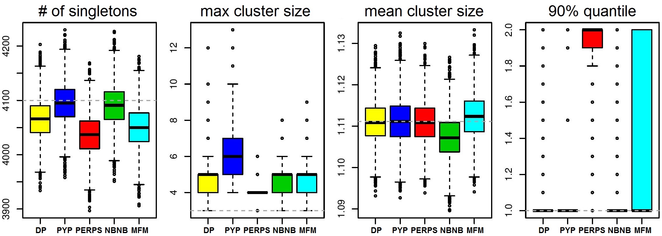
Figure 1: Results for the simulated partition. Each plot contains a boxplot depicting the distribution of a single statistic under each of the five models, obtained using the MLE parameter values (provided in appendix D). The dashed horizontal line indicates the true value of the statistic.

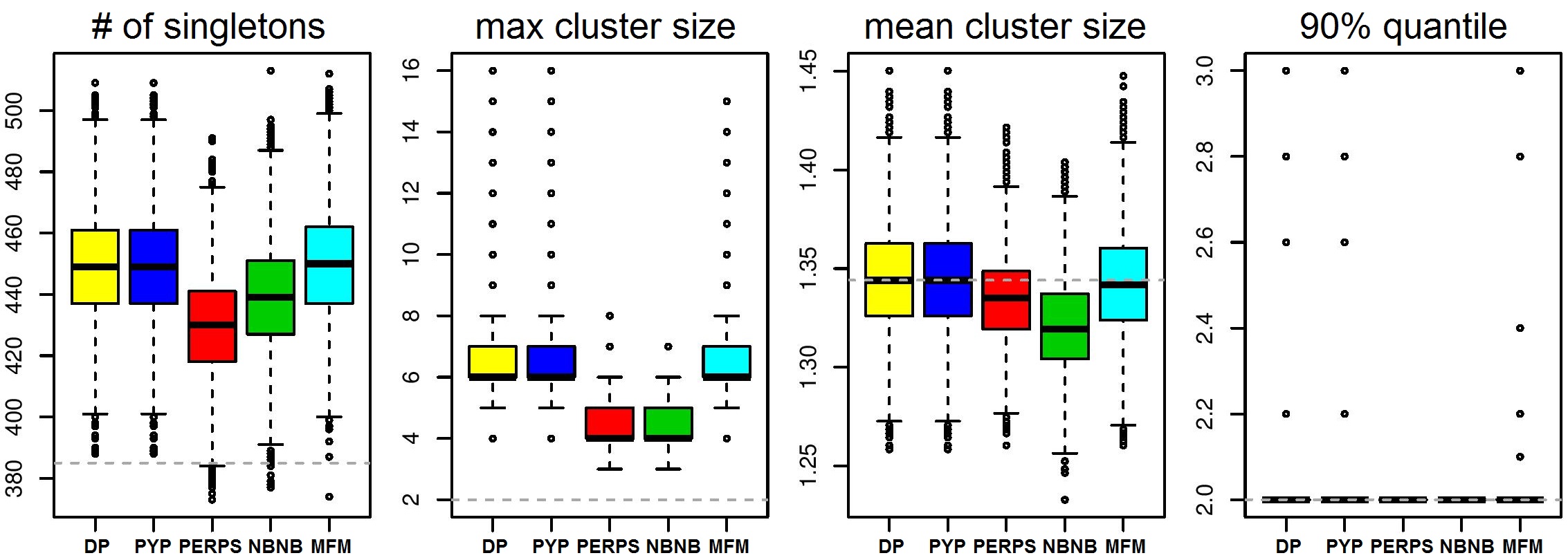
Figure 2: Results for the SHIW partition. This figure’s interpretation is the same as that of figure 1.

5 Discussion

Infinitely exchangeable clustering models assume that cluster sizes grow linearly with the size of the data set. Although this assumption is appropriate for some tasks, many other tasks, including entity resolution, require clusters whose sizes instead grow sublinearly. The microclustering property, introduced in section 2, provides a way to characterize models that address this requirement. The NBNB model, introduced in section 3, exhibits this property. The figures in section 4 show that in some ways—specifically the number of singleton clusters and the maximum cluster size—the NBNB model can fit partitions typical of those arising in entity resolution better than several commonly used mixture models. These results suggest that the NBNB model merits further exploration as a prior for tasks involving clusters whose sizes grow sublinearly with the size of the data set.

Appendix A Derivation of $P(C_{N})$ Under the NBNB and PERPS Models

In this appendix, we derive $P(C_{N})$ where $C_{N}\in\bigcup_{N=0}^{\infty}\mathscr{C}_{N}$. We start by noting that

$$P(C_{N})=\sum_{K=|C_{N}|}^{\infty}P(C_{N}\,|\,K)\,P(K)$$ (5)

and

$$P(C_{N}\,|\,K)=\sum_{z_{1},\ldots,z_{N}\in[K]}\underbrace{P(C_{N}\,|\,z_{1},\ldots,z_{N},K)}_{I(z_{1},\ldots,z_{N}\Rightarrow C_{N})}\,P(z_{1},\ldots,z_{N}\,|\,K)$$ (6)

for any $K\geq|C_{N}|$. (The number of parts in $C_{N}$ may be less than $K$ because some of $N_{1},\ldots,N_{K}$ may be zero.) Since $N_{1},\ldots,N_{K}$ are completely determined by $K$ and $z_{1},\ldots,z_{N}$,

$$P(z_{1},\ldots,z_{N}\,|\,K) =P(z_{1},\ldots,z_{N}\,|\,N_{1},\ldots,N_{K},K)\,P(N_{1},\ldots,N_{K}\,|\,K)$$ (7)

$$=\frac{\prod_{k=1}^{K}N_{k}!}{N!}\prod_{k=1}^{K}P(N_{k}\,|\,K)$$ (8)

$$=\frac{\prod_{k=1}^{K}N_{k}!}{N!}(1-p)^{Kr}\,p^{N}\prod_{k=1}^{K}\frac{r^{(N_{k})}}{N_{k}!},$$ (9)

where we have used $P(N_{k}\,|\,K)=\frac{r^{(N_{k})}}{N_{k}!}(1-p)^{r}\,p^{N_{k}}$. Therefore,

$$P(C_{N}\,|\,K) =\sum_{z_{1},\ldots,z_{N}\in[K]}I(z_{1},\ldots,z_{N}\Rightarrow C_{N})\,\frac{p^{N}}{N!}(1-p)^{Kr}\prod_{k=1}^{K}r^{(N_{k})}$$ (10)

$$=\frac{p^{N}}{N!}(1-p)^{Kr}\left(\prod_{c\in C_{N}}r^{(|c|)}\right)\sum_{z_{1},\ldots,z_{N}\in[K]}I(z_{1},\ldots,z_{N}\Rightarrow C_{N})$$ (11)

$$=\frac{p^{N}}{N!}(1-p)^{Kr}\left(\prod_{c\in C_{N}}r^{(|c|)}\right)\left(|C_{N}|!\right){K\choose|C_{N}|}.$$ (12)

Substituting equation 12 into equation 5 yields

$$P(C_{N})=\frac{p^{N}}{N!}\left(\prod_{c\in C_{N}}r^{(|c|)}\right)\sum_{K=|C_{N}|}^{\infty}(1-p)^{Kr}\left(|C_{N}|!\right){K\choose|C_{N}|}\,P(K).$$ (13)

Using $P(K)=\frac{a^{(K)}}{K!}(1-q)^{a}q^{k}$, we know that

$$\sum_{K=|C_{N}|}^{\infty}(1-p)^{Kr}\left(|C_{N}|!\right){K\choose|C_{N}|}\,P(K)=\frac{(1-q)^{a}\left(q\,(1-p)^{r}\right)^{|C_{N}|}}{\left(1-q\,(1-p)^{r}\right)^{a+|C_{N}|}}\,a^{(|C_{N}|)}.$$ (14)

Finally, substituting equation 14 into equation 13 yields equation 3 as desired.

The PERPS model is similar to the NBNB model (equation 2), but with

$$K\sim\textrm{Poisson}\,(\alpha)\quad\textrm{and}\quad N_{1},\ldots,N_{K}\,|\,K\mathrel{\stackrel{{\scriptstyle\makebox[0.0pt]{\mbox{iid}}}}{{\sim}}}\textrm{Poisson}\,(\lambda),$$ (15)

for $\alpha,\lambda>0$. If we let $r=\lambda\,/\,p$ and $a=\alpha\,/\,q$, and then let $p,q\rightarrow 0$, then equation 3 converges to

$$P_{\textrm{PERPS}}(C_{N})=\frac{\lambda^{N}}{N!}\,\alpha^{|C_{N}|}\,e^{-\alpha}\,e^{-\lambda|C_{N}|}\,e^{\alpha e^{-\lambda}}.$$ (16)

Equation 16 can also be derived directly by following the approach used to derive equation 3.

Appendix B The Chaperones Algorithm: Scalable Inference for Microclustering

For large data sets with many small clusters, standard Gibbs sampling algorithms (such as the one outlined in section 3) are too slow to be used in practice. In this appendix, we therefore propose a new sampling algorithm: the chaperones algorithm. This algorithm is inspired by existing split–merge Markov chain sampling algorithms [14, 4, 6], however, it is simpler, more efficient, and—most importantly—likely exhibits better mixing properties when there are many small clusters.

We start by letting $C_{N}$ denote a partition of $[N]$ and letting $x_{1},\ldots,x_{N}$ denote the $N$ observed data points. In the usual incremental Gibbs sampling algorithm for nonparametric mixture models (described in section 3), each iteration involves reassigning every element (data point) $n=1,\ldots,N$ to either an existing cluster or a new cluster by sampling from $P(C_{N}\,|\,N,C_{N}\setminus n,x_{1},\ldots,x_{N})$. When the number of clusters is large, this step can be very inefficient because the probability that element $n$ will be reassigned to a given cluster will, for most clusters, be extremely small.

Our algorithm focuses on reassignments that have higher probabilities. If we let $c_{n}\in C_{N}$ denote the cluster containing element $n$, then each iteration of our algorithm consists of the following steps:

1. Randomly choose two chaperones, $i,j\in\{1,\ldots,N\}$ from a distribution $P(i,j\,|\,x_{1},\ldots,x_{N})$ where the probability of $i$ and $j$ given $x_{1},\ldots,x_{N}$ is greater than zero for all $i\neq j$. This distribution must be independent of the current state of the Markov chain $C_{N}$; however, crucially, it may depend on the observed data points $x_{1},\ldots,x_{N}$.

2. Reassign each $n\in c_{i}\cup c_{j}$ by sampling from $P(C_{N}\,|\,N,C_{N}\!\setminus\!n,c_{i}\cup c_{j},x_{1},\ldots,x_{N})$.

In step 2, we condition on the current partition of all elements except $n$, as in the usual incremental Gibbs sampling algorithm, but we also force the set of elements $c_{i}\cup c_{j}$ to remain unchanged—i.e., $n$ must remain in the same cluster as at least one of the chaperones. (If $n$ is a chaperone, then this requirement is always satisfied.) In other words, we view the non-chaperone elements in $c_{i}\cup c_{j}$ as “children” who must remain with a chaperone at all times. Step 2 is almost identical to the restricted Gibbs moves found in existing split–merge algorithms, except that the chaperones $i$ and $j$ can also move clusters, provided they do not abandon any of their children. Splits and merges can therefore occur during step 2: splits occur when one chaperone leaves to form its own cluster; merges occur when one chaperone, belonging to a singleton cluster, then joins the other chaperone’s cluster.

This algorithm can be justified as follows: For any fixed pair of chaperones $(i,j)$, step 2 is a sequence of Gibbs-type moves and therefore has the correct stationary distribution. Randomly choosing the chaperones in step 1 amounts to a random move, so, taken together, steps 1 and 2 also have the correct stationary distribution (see, e.g., [15], sections 2.2 and 2.4). To guarantee irreducibility, we start by assuming that $P(x_{1},\ldots,x_{N}\,|\,C_{N})\,P(C_{N})>0$ for any $C_{N}$ and by letting $C^{\prime}_{N}$ denote the partition of $N$ in which every element belongs to a singleton cluster. Then, starting from any partition $C_{N}$, it is easy to check that there is a positive probability of reaching $C^{\prime}_{N}$ (and vice versa) in finitely many iterations; this depends on the assumption that $P(i,j\,|\,x_{1},\ldots,x_{N})>0$ for all $i\neq j$. Aperiodicity is also easily verified since the probability of staying in the same state is positive.

The main advantage of the chaperones algorithm is that it can exhibit better mixing properties than existing sampling algorithms. If the distribution $P(i,j\,|\,x_{1},\ldots,x_{N})$ is designed so that $x_{i}$ and $x_{j}$ tend to be similar, then the algorithm will tend to consider reassignments that have a relatively high probability. In addition, the algorithm is easier to implement and more efficient than existing split–merge algorithms because it uses Gibbs-type moves, rather than Metropolis-within-Gibbs moves.

Appendix C NBNB and the Microclustering Property

In this appendix, we present empirical evidence that suggests that the sequence of partitions implied by the NBNB model exhibits the microclustering property. Figure 3 shows $M_{N}\,/\,N$ for samples of $M_{N}$ over a range of $N$ values from ten to $10^{4}$. We obtained each sample of $M_{N}$ using the NBNB model with $a=1$, $q=0.9$, and $r,p$ such that $\mathbb{E}(N_{k}\,|\,K)=3$ and $\textrm{var}\,(N_{k}\,|\,K)=3^{2}\,/\,2$. For each value of $N$, we initialized the algorithm with the partition in which all elements are in a single cluster. We then ran the reseating algorithm in section 3 for 1,000 iterations to generate $C_{N}$ from $P(C_{N}\,|\,N)$, and set $M_{N}$ to the size of the largest cluster in $C_{N}$. As $N\rightarrow\infty$, $M_{N}\,/\,N$ appears to converge to zero in probability, suggesting that the model exhibits the microclustering property.

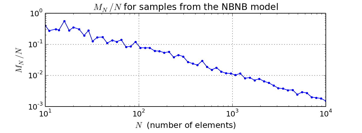
Figure 3: Empirical evidence suggesting that the NBNB model exhibits the microclustering property.

Appendix D Experiments

For each data set, we calculated each model’s MLE parameter values using the Nelder–Mead algorithm. For the simulated partition, the MLE values are $r=2.955\times 10^{-5}$, $p=0.1875$, $a=102.4$, and $q=0.9999$ for the NBNB model; $\lambda=0.215$ for the PERPS model; $\gamma=0.279$ for the MFM model; $\theta=21,\!719$ for the DP model; and $\theta=9,\!200$ and $\delta=0.540$ for the PYP model. For the SHIW partition, the MLE values are $r=1,\!001$, $p=6.212\times 10^{-4}$, $a=100.6$, and $q=0.9267$ for the NBNB model; $\lambda=0.624$ for the PERPS model; $\gamma=1.056\times 10^{-2}$ for the MFM model; $\theta=1,\!037$ for the DP model; and $\theta=1,\!037$ and $\delta=0$ for the PYP model (making it identical to the DP model). Note that for both data sets, the DP and PYP concentration parameters are very large.

References

- [1] P. Christen. Data Matching: Concepts and Techniques for Record Linkage, Entity Resolution, and Duplicate Detection. Springer, 2012.
- [2] P. Christen. A survey of indexing techniques for scalable record linkage and deduplication. IEEE Transactions on Knowledge and Data Engineering, 24(9), 2012.
- [3] W. E. Winkler. Overview of record linkage and current research directions. Technical report, U.S. Bureau of the Census Statistical Research Division, 2006.
- [4] R. C. Steorts, R. Hall, and S. E. Fienberg. A Bayesian approach to graphical record linkage and de-duplication. Journal of the American Statistical Society, In press.
- [5] R. C. Steorts. Entity resolution with empirically motivated priors. Bayesian Analysis, 10(4):849–875, 2015.
- [6] R. C. Steorts, R. Hall, and S. E. Fienberg. SMERED: A Bayesian approach to graphical record linkage and de-duplication. Journal of Machine Learning Research, 33:922–930, 2014.
- [7] S. Richardson and P. J. Green. On Bayesian analysis of mixtures with an unknown number of components. Journal of the Royal Statistical Society Series B, pages 731–792, 1997.
- [8] J. W. Miller and M. T. Harrison. Mixture models with a prior on the number of components. arXiv:1502.06241, 2015.
- [9] J. Sethuraman. A constructive definition of Dirichlet priors. Statistica Sinica, 4:639–650, 1994.
- [10] H. Ishwaran and L. F. James. Generalized weighted Chinese restaurant processes for species sampling mixture models. Statistica Sinica, 13(4):1211–1236, 2003.
- [11] J. F. .C Kingman. The representation of partition structures. Journal of the London Mathematical Society, 2(2):374–380, 1978.
- [12] D. Aldous. Exchangeability and related topics. École d’Été de Probabilités de Saint-Flour XIII—1983, pages 1–198, 1985.
- [13] H. M. Wallach, S. Jensen, L. Dicker, and K. A. Heller. An alternative prior process for nonparametric Bayesian clustering. In Proceedings of the 13 International Conference on Artificial Intelligence and Statistics, 2010.
- [14] S. Jain and R. Neal. A split–merge Markov chain Monte Carlo procedure for the Dirichlet process mixture model. Journal of Computational and Graphical Statistics, 13:158–182, 2004.
- [15] L. Tierney. Markov chains for exploring posterior distributions. The Annals of Statistics, pages 1701–1728, 1994.