A study of excess energy and decoherence factor of a qubit coupled to a one dimensional periodically driven spin chain

Abstract

We take a central spin model (CSM), consisting of a one dimensional environmental Ising spin chain and a single qubit connected globally to all the spins of the environment, to study numerically the excess energy (EE) of the environment and the logarithm of decoherence factor namely, dynamical fidelity susceptibility per site (DFSS), associated with the qubit under a periodic driving of the transverse field term of environment across its critical point using the Floquet technique. The coupling to the qubit, prepared in a pure state, with the transverse field of the spin chain yields two sets of EE corresponding to the two species of Floquet operators. In the limit of weak coupling, we derive an approximated expression of DFSS after an infinite number of driving period which can successfully estimate the low and intermediate frequency behavior of numerically obtained DFSS. Our main focus is to analytically investigate the effect of system-environment coupling strength on the EEs and DFSS and relate the behavior of DFSS to EEs as a function of frequency by plausible analytical arguments. We explicitly show that the low-frequency beating like pattern of DFSS is an outcome of two frequencies, causing the oscillations in the two branches of EEs, that are dependent on the coupling strength. In the intermediate frequency regime, dip structure observed in DFSS can be justified by the resonance peaks of EEs at those coupling parameter dependent frequencies; high frequency saturation value of EEs and DFSS are also connected to each other by the coupling strength.

I Introduction

Dynamics of a periodically driven closed quantum system has been studied extensively in recent years. These studies are truly interdisciplinary in nature and are being carried out from the viewpoint of quenching dynamics of many body quantum systems zurek05 ; polkovnikov05 ; damski05 ; mukherjee07 ; mukherjee09 ; dziarmaga10 ; polkovnikov11 and the quantum information theorybarankov08 ; sengupta09 ; quan10 ; nag11 ; nag12a ; mukherjee12 ; suzuki15 . The behavior of these quantum systems are very much different when compared to the classical periodically driven systems shirley65 ; grossmann91 ; hanggi98 ; kayanuma94 ; canovi12 ; russomanno12 . Many interesting phenomena like coherent destruction of tunnelingdas10 , a periodic steady state behavior of various thermodynamic observablesrussomanno12 ; bastidas12 ; russomanno13 and dynamical localizationlazarides14 ; nag14 ; nag15 , etc., manifest in a periodically driven quantum system. A lot of attention has been paid to Floquet technique due to its successful execution in many periodically driven systems such as Floquet Graphenegu11 ; kitagawa11 , Floquet topological insulatorgomez12 ; some of them have also been realized experimentally kitagawa12 . Moreover, the excess energy (EE) and the work distribution function for the transverse Ising model subjected to a time periodic variation of transverse field have also been studied extensively using Floquet technique russomanno15 .

Given the recent interest in quenching dynamics of quantum systems, there has been a plethora of studies connecting quantum information theorynielsen00 ; vedral07 to the quantum critical systemchakrabarti96 ; sachdev99 ; dutta15 . The loss of coherence in a quantum system due to its interaction with the environment namely, decoherence, quantified as decoherence factor (DF) also known as Loschmidt echo, is an emerging topic that has been studied greatly in this regardzurek03 ; quan06 . The quenching dynamics of the DFdamski11a ; nag12b ; roy13 ; sachdeva14 has also been investigated throughly for integrable as well as non-integrable quantum system under the scope of a central spin model (CSM)CSM1 ; cucchietti07 ; venuti10 ; suzuki15 . Importantly, in this connection, it has been shown that decohered density matrix of a quantum system under consideration might not always result in the accurate behavior of dynamical fidelity susceptibility per site (DFSS), defined through the logarithm of squared modulus overlap between the initial state and the time-evolved final state, in the infinite time limit while the quantum system is periodically driven across its QCPsharma14 . Furthermore, there is an experimental observation of quantum criticality has been made by investigating the behavior of Loschmidt echo, measured without associating an external qubit, in an antiferromagnetic Ising spin chain with finite number of spins using NMR quantum simulator zhang09 .

We shall consider here a CSM with an environment as 1-d transverse Ising spin chain and a single qubit, weakly and globally coupled to the transverse field term of the chain, to investigate the non trivial effect caused by the coupling parameter on the behavior of the EE of that periodically driven environment across its QCP. Consequently, this coupling leads to two channels of time evolution for the environment with the modified transverse fields. These phenomena allows us to exclusively probe the decohering phenomena of the qubit by examining the DFSS as a function of frequency. In contrast to the Ref. [sharma14, ] where the overall loss of phase coherence of a periodically driven spin chain across its QCP has been studied using the Floquet technique, our main focus is to probe the effect of the coupling parameter on DFSS, quantified through the ratio of logarithm of the modulus squared overlap between two states reached after an infinite number of period of time evolution with two environmental channels and system size of the environment, of the external qubit under a sinusoidal driving of the transverse field across the QCP. To the best of our knowledge, this is the first work to examine the behavior of the DFSS of a qubit using the Floquet technique under the scope of CSM. Most interestingly, we show that the behavior of DFSS can be characterized by analyzing the behavior of EEs associated to the two evolution channels of the spin chain environment in different frequency regimes.

The paper is organized in the following way. In Sec. (II), we introduce the transverse Ising spin chain and the corresponding central spin model where a single qubit is considered as the system with the spin chain acting as an environment. In parallel, we present Floquet technique and express the wave-function for a periodically driven system in the Floquet representation. We also elaborately discuss the Floquet machinery in our case to probe the EEs of the environment and the DFSS of the system. In Sec. (III), We analyze the behavior of quasi-energy, EE and DFSS, obtained numerically, by explicit analytical calculations with the plausible argument. Finally, we present concluding comments in Sec. (IV).

II Model and Floquet Technique

The Hamiltonian $H_{E}$ of the environment is the ferromagnetic Ising spin chain in a transverse field consisting of $N$ spins given by bunder99

$$H_{E}=-\sum_{i=1}^{N}[\sigma_{i}^{x}\sigma_{i+1}^{x}+h\sigma_{i}^{z}],$$ (1)

where $\sigma_{x}$ and $\sigma_{z}$ are the Pauli matrices. This model can be exactly solved by mapping the spins to spinless Fermion through Jordon-Wigner transformation bunder99 ; lieb61 . The model can be decomposed to $2\times 2$ Hamiltonian in the momentum space under periodic boundary condition. The momentum space Hamiltonian is given by,

$${\cal H}^{E}_{k}=\left[\begin{array}[]{cc}-h(t)+\cos k&\sin k\\ \sin k&h(t)-\cos k\end{array}\right],$$ (2)

The model has quantum phase transitions (QPTs) at $h=\pm 1$. This QCP belongs to Ising universality class with $\nu=1$ and $z=1$, where $\nu$ is the correlation length exponent and $z$ is the dynamical exponent. This model has a ferromagnetic phase for $|h|<1$ and a paramagnetic phase for $|h|>1$. In our case, the transverse field is being subjected to a time periodic sinusoidal driving: $h(t)=1+h_{0}\cos(\omega t)$, where $h_{0}$ is the amplitude of the driving and $\omega=2\pi/T$ is the frequency of the driving with time period $T$. In our ramp protocol, spin chain experiences the QPT only at $h=1$ as the transverse field $h$ is varied between $2$ and $0$.

Let us now discuss the central spin model in which a single spin-$1/2$ particle (qubit) is globally connected to all the spins of the environmental spin chain with an interaction Hamiltonian $H_{SE}=\delta\sum_{i=1}^{N}\sigma_{i}^{z}\sigma_{S}^{z}$, where $\sigma_{i}^{z}$ is the $i-$th spin of the $XY$ chain, $\sigma_{S}^{z}$ represents that of the qubit and $\delta$ is the coupling strength. Here, we consider that the transverse field initially at $t=0^{-}$ is $h=1+h_{0}$ and the coupling to the qubit is suddenly made at $t=0^{+}$ and simultaneously the sinusoidal driving is being started.

We choose the qubit to be initially in a pure state at $t=0$, $|\phi_{S}(t=0)\rangle=a_{+}|\uparrow\rangle+a_{-}|\downarrow\rangle$, where $|\uparrow\rangle$ and $|\downarrow\rangle$ represent up and down states of the qubit, respectively, and the environment is in the ground state $|\phi_{E}(t=0)\rangle=|\phi_{g}\rangle$. The ground state of the composite Hamiltonian $H_{E}+H_{SE}$, at $t=0$, is then given by their direct product

$$|\psi(t=0)\rangle=|\phi_{S}(t=0)\rangle\otimes|\phi_{g}\rangle.$$ (3)

It can be shown that at a later time $t$, the composite wave-function is given by damski11a

$$|\psi(t)\rangle=a_{+}|\uparrow\rangle\otimes|\phi(+,t)\rangle+a_{-}|\downarrow\rangle\otimes|\phi(-,t)\rangle,$$ (4)

where $|\phi(\pm,t)\rangle$ are the environmental wave-functions, satisfying the time dependent schrödinger equation: $i|\dot{\phi}(\pm,t)\rangle=H_{E}(h(t)\pm\delta)|\phi(\pm,t)\rangle$, evolved from the initial ground state wave-function $|\phi_{g}(t=0^{-})\rangle$ before the qubit gets coupled to the environment. The form of the interaction Hamiltonian generates two evolution channels with the modified transverse field as $(h(t)\pm\delta)$. Therefore, the modified Hamiltonians ${\mathcal{H}}^{E}_{k}(\pm,t)$ which govern the time evolution of environmental spin chain in momentum space is given by

$$\mathcal{H}^{E}_{k}(\pm,t)=\left[\begin{array}[]{cc}-h(t)\mp\delta+\cos k&\sin k\\ \sin k&h(t)\pm\delta-\cos k\end{array}\right],$$ (5)

We can now focus on the Floquet theory for a generic time-periodic Hamiltonian, $H\left(t\right)=H\left(t+T\right)$. One can construct a time evolution operator for a single period which is referred as the Floquet operator ${\cal F}={\mathcal{O}}e^{-i\int_{0}^{T}H(t)dt}$, where $\mathcal{O}$ denotes time-ordering. $\hbar$ is set to unity. The solution of the Schrödinger equation for the $j$-th state in the Floquet basis ($|\eta_{j}(t)\rangle$ which are eigenstates of ${\cal F}$) can be written in the form $|\Psi_{j}(t)\rangle=e^{-i\mu_{j}t}|\eta_{j}(t)\rangle$. The states $|\eta_{j}(t)\rangle$’s are time periodic ($|\eta_{j}(t)\rangle=|\eta_{j}(t+T)\rangle$) and $e^{-i\mu_{j}T}$ are the corresponding eigenvalues of ${\cal F}$; the $\mu_{j}$’s are called Floquet quasi-energies. Now, making use the fact that the environmental spin chain reduces to $2\times 2$ momentum space Hamiltonian, one can construct a momentum space Floquet operator ${\mathcal{F}}_{k}$ at the stroboscopic time $t=T$. For a sinusoidally varying parameter, one has to numerically find out the Floquet operator starting from a generic state $(0~{}1)^{\mathcal{T}}$, $\mathcal{T}$ denotes the transpose of a matrix. The time evolved wave-function at $t=T$ is given by $(u_{k}~{}v_{k})^{\mathcal{T}}$. Therefore, the ${\mathcal{F}}_{k}$ can be constructed from the above state, satisfying the constraint that ${\mathcal{F}}_{k}(t=0)$ is an identity, is given by

$$\mathcal{F}_{k}=\left[\begin{array}[]{cc}u_{k}&-v_{k}^{*}\\ v_{k}&u_{k}^{*}\end{array}\right],$$ (6)

Now in our case, one can get two Floquet operators $\mathcal{F}_{k}(\pm)$ for two channels of evolution associated with the modified transverse fields $h(t)\pm\delta$. By diagonalizing the Floquet operators one can get $\mu_{k}^{\pm}(\pm)$, quasi-energies and $|\eta_{k}^{\pm}(\pm)\rangle$, quasi-states corresponding to two channels of evolution. ($\mathcal{F}_{k}(+)$ gives two quasi-states $|\eta_{k}^{\pm}(+)\rangle$, same as for the negative channel). Under the periodic driving, the time evolved environmental state $|\phi_{k}(\pm)\rangle$ at time $t=nT$, can be obtained in terms of Floquet basis sates,

$$|\phi_{k}(\pm,nT)\rangle = c_{k}^{+}(\pm)\mathrm{e}^{-i\mu_{k}^{+}(\pm)\,nT}|\eta_{k}^{+}(\pm)\rangle$$ (7)

$$+ c_{k}^{-}(\pm)\mathrm{e}^{-i\mu_{k}^{-}(\pm)\,nT}|\eta_{k}^{-}(\pm)\rangle,$$

where $c_{k}^{\pm}(\pm)=\langle\eta_{k}^{\pm}(\pm)|\phi_{g,k}\rangle$, with $|\phi_{g,k}\rangle$ is the initial bare ground state of the environment for a momentum mode $k$ at $t=0^{-}$ when the qubit is not coupled with the environment.

We can now probe the EE and DFSS as a function of frequency by using environmental wave-function. We have two sets of EE, associated with the two channels of time evolution, are given by

$$W(\pm,nT) = (1/N)\sum_{k}W_{k}(\pm,nT)\equiv(1/N)\sum_{k}[e_{k}(\pm,nT)$$ (8)

$$- e_{g,k}(\pm,nT)],$$

where $e_{k}(\pm,nT)$ is the energy expectation value of the environmental Hamiltonian (5) for the $k$-th mode, reached after $n$-th time period, given by $e_{k}(\pm,nT)=\langle\phi_{k}(\pm,nT)|\mathcal{H}^{E}_{k}(\pm,nT)|\phi_{k}(\pm,nT)\rangle$; $e_{g,k}(\pm,nT)$ is the ground state energy of the ${\mathcal{H}}^{E}_{k}(\pm,nT)$.

In the limit of $n\to\infty$, we resort to the Riemann-Lesbesgue lemma for integrating out the rapidly oscillating phase factor. The EEs for the two channels by retaining only the steady state contribution in infinite time limit are given by

$$W(\pm) = (1/N)\sum_{k}\biggl{[}|c_{k}^{+}(\pm)|^{2}\langle\eta_{k}^{+}(\pm)|H(\pm,T)|\eta_{k}^{+}(\pm)\rangle$$ (9)

$$+ |c_{k}^{-}(\pm)|^{2}\langle\eta_{k}^{-}(\pm)|H(\pm,T)|\eta_{k}^{-}(\pm)\rangle$$

$$- e_{g,k}(\pm,T)\biggr{]}$$

We shall now find out the DF of the qubit from the reduced density matrix of the qubit by tracing over environmental part from the composite density matrix. The reduced density matrix in the ${\{|\uparrow\rangle,|\downarrow\rangle\}}$ basis reads as

$$\mathcal{\rho}_{S}(t)={\rm Tr}_{\cal E}\biggl{[}|\psi(t)\rangle\langle\psi(t)|\biggr{]}=\left[\begin{array}[]{cc}|a_{+}|^{2}&a_{+}a_{-}^{*}d^{*}(t)\\ a_{+}^{*}a_{-}d(t)&|a_{-}|^{2}\end{array}\right],$$ (10)

where $d(t)=\langle\phi_{+}(t)|\phi_{-}(t)\rangle$ appears as an off-diagonal element in the reduced density matrix and is related to the DF $D(t)$ by a modulo square of $d(t)$damski11a , $D(t)=|\langle\phi_{+}(t)|\phi_{-}(t)\rangle|^{2}$. DF measures the purity of the qubit; $D=1$ signifies that the qubit is in a pure state.

In the momentum space language, $D(t)$ is given by $D(t)=\Pi_{k>0}|d_{k}(t)|^{2}=\Pi_{k>0}|\langle\phi_{k}(+,t)|\phi_{k}(-,t)\rangle|^{2}$. Similarly, one can measure the DF of qubit after $n$-th cycle of the time periodic transverse field. Therefore, the DF in its rudimentary form is therefore given by

$$D(n) =\Pi_{k>0}D_{k}(n)$$ (11)

$$= \Pi_{k>0}\biggl{[}|c_{k}^{+}(+)|^{2}|c_{k}^{+}(-)|^{2}~{}|\langle\eta_{k}^{+}(+)|\eta_{k}^{+}(-)\rangle|^{2}$$

$$+ |c_{k}^{-}(+)|^{2}|c_{k}^{-}(-)|^{2}~{}|\langle\eta_{k}^{-}(+)|\eta_{k}^{-}(-)\rangle|^{2}$$

$$+ |c_{k}^{+}(+)|^{2}|c_{k}^{-}(-)|^{2}|\langle\eta_{k}^{+}(+)|\eta_{k}^{-}(-)\rangle|^{2}$$

$$+ |c_{k}^{-}(+)|^{2}|c_{k}^{+}(-)|^{2}|\langle\eta_{k}^{-}(+)|\eta_{k}^{+}(-)\rangle|^{2}$$

$$+ 2~{}{\rm Re}\biggl{[}T^{\prime}_{1}+T^{\prime}_{2}+T^{\prime}_{3}+T^{\prime}_{4}+T^{\prime}_{5}+T^{\prime}_{6}\biggr{]}\biggr{]},$$

where the $T_{m}$’s denote the cross terms which come in pairs. Here, we use $T^{\prime}_{m}+(T^{\prime}_{m})^{*}=2~{}{\rm Re}[T^{\prime}_{m}]$. For our convenience, we shall segregate the exponential part from the $T^{\prime}_{m}$ i.e., $T^{\prime}_{m}=T_{m}\times{\rm exp}(i\alpha_{m})$. $T_{m}$’s and $\alpha_{m}$’s are given by

$$T_{1} = c_{k}^{+}(+)^{*}c_{k}^{+}(-)c_{k}^{-}(+)c_{k}^{-}(-)^{*}\langle\eta_{k}^{+}(+)|\eta_{k}^{+}(-)\rangle$$

$$\times \langle\eta_{k}^{-}(-)|\eta_{k}^{-}(+)\rangle,$$

$$T_{2} = |c_{k}^{+}(+)|^{2}c_{k}^{-}(-)^{*}c_{k}^{+}(-)\langle\eta_{k}^{+}(+)|\eta_{k}^{+}(-)\rangle\langle\eta_{k}^{-}(-)|\eta_{k}^{+}(+)\rangle,$$

$$T_{3} = |c_{k}^{+}(-)|^{2}(c_{k}^{+}(+))^{*}c_{k}^{-}(+)\langle\eta_{k}^{+}(+)|\eta_{k}^{+}(-)\rangle\langle\eta_{k}^{+}(-)|\eta_{k}^{-}(+)\rangle,$$

$$T_{4} = |c_{k}^{-}(-)|^{2}c_{k}^{-}(+)^{*}c_{k}^{+}(+)\langle\eta_{k}^{-}(+)|\eta_{k}^{-}(-)\rangle\langle\eta_{k}^{-}(-)|\eta_{k}^{+}(+)\rangle,$$

$$T_{5} = |c_{k}^{-}(+)|^{2}c_{k}^{+}(-)^{*}c_{k}^{-}(-)\langle\eta_{k}^{-}(+)|\eta_{k}^{-}(-)\rangle\langle\eta_{k}^{+}(-)|\eta_{k}^{-}(+)\rangle,$$

$$T_{6} = c_{k}^{+}(+)^{*}c_{k}^{-}(-)c_{k}^{-}(+)c_{k}^{+}(-)^{*}\langle\eta_{k}^{+}(+)|\eta_{k}^{-}(-)\rangle$$

$$\times \langle\eta_{k}^{+}(-)|\eta_{k}^{-}(+)\rangle,$$

$$\alpha_{1} = 2nT(\mu_{k}^{+}(+)-\mu_{k}^{+}(-)),~{}\alpha_{2}=-2nT\mu_{k}^{+}(-),$$

$$\alpha_{3} = 2nT\mu_{k}^{+}(+),~{}\alpha_{4}=-2nT\mu_{k}^{+}(+),$$

$$\alpha_{5} = -2nT\mu_{k}^{-}(-),~{}\alpha_{6}=2nT(\mu_{k}^{+}(+)-\mu_{k}^{-}(-))$$

Our main aim is to study the behavior of DFSS given by $\chi_{F}(n\to\infty)=\log(D(n\to\infty))/N=\sum_{k}{\rm log}(D_{k}(n\to\infty))/N$ in the infinite time limit. We note the DF of the qubit is appreciably small referring to the fact that the qubit is totally in a mixed state after an infinite number of periods and hence, the logarithm of DF namely, fidelity susceptibility is the main quantity to be studied in this context. The first four terms of the above expression (11) give the decohered value which is not the actual value of the DFSS in the $n\to\infty$ limit. In this limit one can not simply neglect the exponential term, appearing inside the logarithm, of DFSS sharma14 .

One can consider $T_{m}$ is a real quantity without loss of generality. Now, in order to simplify the expression in $n\to\infty$ limit we shall write the $\chi_{F}(n)$ in the following form

$$\chi_{F}(n)={1\over N}\sum_{k}\biggl{[}\log(D^{\rm dec}_{k})+\log\biggl{(}1+\sum_{m=1}^{6}({x^{\prime}_{m}}\cos\alpha_{m})\biggr{)}\biggr{]}$$ (12)

where $x^{\prime}_{m}=2T_{m}/D^{\rm dec}_{k}$, and $D_{k}^{\rm dec}$ is the decohered part, consisting of first four terms in Eq. (11), for a momentum mode $k$ .

Now, in the limit of sufficiently smaller value of $\delta$ and using the asymptotic expansion of logarithmic series $\log(1+x)\simeq x-x^{2}/2+x^{3}/3-\cdots$, one can use the Riemann- Lesbesgue lemma to achieve the final form of the DFSS in the $n\to\infty$ limit sharma14 . The fidelity susceptibility $\chi_{F}$ is defined as $F(\lambda,\lambda+\delta)=|\langle\psi_{0}(\lambda)|\psi_{0}(\lambda+\delta)\rangle|^{2}=1-\delta^{2}N\chi_{F}$, where $|\psi_{0}(\lambda)\rangle$ is the ground state of the quantum systemzanardi06 . Therefore, one can express $\chi_{F}(n\to\infty)$ up to $O(\delta^{2})$ in the power series of $x^{\prime}_{m}$’s

$$\chi_{F}(\infty) \simeq \int{dk\over 2\pi}\biggl{[}\log D^{\rm dec}_{k}-\biggl{(}{x^{\prime 2}_{1}\over 4}+{3x^{\prime 4}_{1}\over 32}+{5x^{\prime 6}_{1}\over 96}+\cdots$$ (13)

$$+ \sum_{m=2}^{6}{x^{\prime 2}_{m}\over 4}\biggr{)}+{\rm cross~{}terms}\biggr{]}$$

$$\approx \int{dk\over 2\pi}\biggl{[}\log D^{\rm dec}_{k}-\biggl{(}\log\biggl{(}{2\over 1+\sqrt{1-x^{\prime 2}_{1}}}\biggr{)}$$

$$+ \sum_{m=2}^{5}{x^{\prime 2}_{m}\over 4}\biggr{)}\biggr{]}$$

The detail of the above derivation to obtain the simplified and approximated expression of $\chi_{F}(\infty)$ (13) is presented in the Appendix (A).

Here, we use the fact that any even multiple of $\cos\alpha_{m}$ would contribute to the integral as they do not average to zero when $n$ is very large. The cross terms in the $\chi_{F}(\infty)$ are sum of the product of $x^{\prime a}_{m}$ and $x^{\prime b}_{n}$ with their all possible combinations where $a$ and $b$ are both even numbers and $m\neq n$. In the low frequency and intermediate frequency regime the product terms $x^{\prime}_{1}x^{\prime}_{m}$ (with $m\neq 1$) are infinitesimally small and contribution coming from $x^{\prime a}_{1}x^{\prime 2}_{m}$ can be safely neglected; consequently, the $\chi_{F}(\infty)$ is sufficient to estimate the behavior exhibited by $\log(D(n))/N$ which is obtained numerically using a large value of $n$. Therefore, excluding the above “cross terms” we keep up to an $O(\delta^{2})$ term, coming from the decohered part, logarithmic part and $x^{\prime 2}_{m}$ (with $m=2,~{}\cdots,~{}5$), in calculating $\chi_{F}(\infty)$ with small but finite $\delta<1$.

One can numerically check that the $x^{\prime}_{1}x^{\prime}_{m}$ has a significant contribution in the high frequency regime and $x^{\prime a}_{1}x^{\prime 2}_{m}$ can not be neglected. This might cause a problem for the approximated expression of $\chi_{F}(\infty)$ (13) in determining the accurate behavior obtained numerically by $\chi_{F}(n)=\log(D(n))/N$ (12) with a large value of $n$ in that high frequency limit.

Furthermore, one can not simply obtain $\chi_{F}(\infty,\delta)=0$ by setting $\delta=0$ in $\chi_{F}(\infty)$ (13). One has to separately treat the infinitesimally small $\delta\to 0$ case. In order to probe $\delta=0$ limit, $\chi_{F}(n)$ (12) is the appropriate quantity to begin with. In the case of $\delta=0$, we have only one Floquet operator and as a result $|\eta_{k}^{\pm}(-)\rangle=|\eta_{k}^{\pm}(+)\rangle=|\eta_{k}^{\pm}\rangle$, $\mu_{k}^{\pm}(+)=\mu_{k}^{\pm}(-)=\mu_{k}^{\pm}$ and $c_{k}^{\pm}(+)=c_{k}^{\pm}(-)=c_{k}^{\pm}$. Therefore, $T^{\prime}_{1}$ is the only non-decohered term which contributes to the $\chi_{F}(n)$ (12); all the other cross terms $T^{\prime}_{m}$, $m\neq 1$, vanish due the orthogonality condition of quasi-states $\langle\eta_{k}^{+}|\eta_{k}^{-}\rangle=0$. It can be easily shown that $\chi_{F}(n)$ for $\delta=0$ reduces to the following form

$$\chi_{F}(n,\delta=0) = {1\over N}\sum_{k}\log\biggl{(}|c_{k}^{+}|^{4}+|c_{k}^{-}|^{4}+2|c_{k}^{+}|^{2}|c_{k}^{-}|^{2}\biggr{)}$$ (14)

$$= {1\over N}\sum_{k}\log\biggl{(}\biggl{[}|c_{k}^{+}|^{2}+|c_{k}^{-}|^{2}\biggr{]}^{2}\biggr{)}=0$$

Since, $\chi_{F}(n,\delta=0)$ (14) does not have any sinusoidal term containing $n$ in its argument; this allows us to write $\chi_{F}(n\to\infty,\delta=0)=\chi_{F}(n,\delta=0)=0$.

Interestingly, the $\chi_{F}(\infty)$ (13) can not correctly quantify the DFSS when $\delta=0$ as the $\log(D_{k}^{\rm dec})$ and $\log(2/(1+\sqrt{1-x^{\prime 2}_{1}}))$ terms of order $O(\delta^{0})$ do not cancel each other. In order to obtain the $\chi_{F}(\infty)$ (13), we replace the even power of sinusoidal term by its time averaged value and this results in a permanent loss of phase information while calculating $\chi_{F}(n\to\infty)$. The loss of phase information causes the irreversibility in the behavior of $\chi_{F}(\infty)$ i.e., $\chi_{F}(n)$ can successfully predict the $\delta=0$ behavior where as $\chi_{F}(\infty)$, derived from $\chi_{F}(n)$ with $n\to\infty$, can not correctly quantify the $\delta=0$ behavior.

III Results

In this section, we examine the nature of quasi-energies, EEs and the DFSS in detail. We shall first investigate the behavior of the two sectors of quasi-energies associated with the two coupling channels as a function of the momentum. The time periodic Hamiltonian causes a temporal Brillouin zone (TBZ) structure of width $\omega$ in the behavior of quasi-energy $\mu_{k}^{\pm}(\pm)$ and consequently this originates the quasi-degeneracy in the Floquet spectrum hanggi98 . Quasi-degeneracy occurs when the one branch of the Floquet spectrum meets with the other branch inside the same TBZ or two adjacent TBZs. Investigating each channel of quasi-energy (see Fig. 1 (a) and (b)), we find that the coupling strength $\delta$ indeed has an effect on quasi-degenerate momentum mode.

In order to find out the quasi-degenerate momentum value we have to take the limit $h_{0}\to 0$ in Eq. (5). Therefore, the quasi-degeneracy condition can be obtained by diagonalizing the Hamiltonian (5) is given by

$$E_{k}(\pm)=-E_{k}(\pm)+l\omega,~{}~{}l=0,1,2,\cdots$$ (15)

where $E_{k}(\pm)$ is eigenvalue of Hamiltonian (5) in the limit $h_{0}\to 0$. Therefore, quasi-degenerate momentum modes $k^{\pm}_{q}(\delta)\simeq 2\arcsin((1\pm\delta/2)~{}l\omega/4)$ which are quantitatively matching with the quasi-degenerate momentum observed in Fig. (1a). The point to note is that there is no quasi-degeneracy exists for $k=0$ and $\pi$ due to the coupling $\delta$. The $k^{+}_{q}(\delta)(k^{-}_{q}(\delta))$ for positive (negative) channel gets shifted towards right (left) of the $k_{q}(\delta=0)$. This shifting is observed quite prominently as one increases $k$ from $0$ to $\pi$.

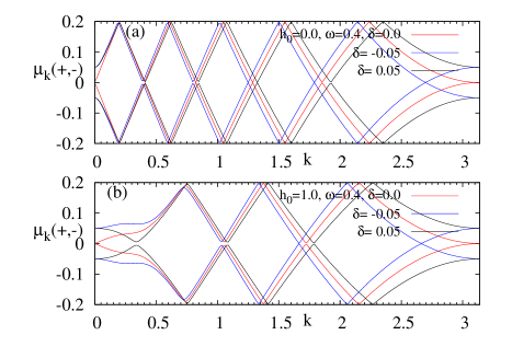
Figure 1: Fig. (a) shows the variation of two channels of quasi-energy $\mu_{k}^{\pm}(\pm)$ as a function of momentum $k$ with driving amplitude $h_{0}=0$. Fig. (b) depicts the behavior of quasi-energy while the driving amplitude is finite $h_{0}=1$.

Similarly, we show in Fig. (1b) that $k^{\pm}_{q}(\delta)$ shifts towards the Brillouin zone (BZ) boundary $k=\pi$ for higher value of $h_{0}=1$. As a result, less number of quasi-degeneracy appears in Floquet spectrum. Figure (3) shows that the EEs exhibit peaks at those quasi-degenerate points for finite $h_{0}$. Hereafter, we shall refer positive channel as $\delta>0$ and negative channel as $\delta<0$ in all the figure.

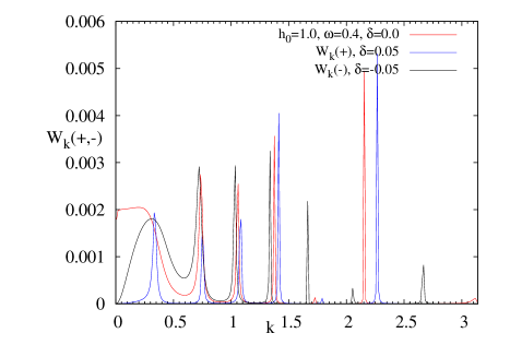
Figure 2: Plot shows the variation of EEs $W_{k}(\pm)$ for two channels with modified ($h(t)\pm\delta$) as a function of $k$.

Now, we shall focus on the behavior of the two channels of EE $W(\pm)$, obtained numerically from Eq. (9), as a function of frequency $\omega$. Hereafter, we set $h_{0}=1$. We divide the frequency range into three parts depending upon the distinctive behavior of EE in these $\omega$ regimes, (a) low-frequency oscillations of $W(\pm)$, (b) resonance peak of $W(\pm)$ at the intermediate frequency and (c) high frequency plateau of EE. In all of the above three regions the coupling strength $\delta$ plays an important role in determining the behavior of $W(\pm)$.

Let us first explore the part (a) i.e., the low-frequency regime. By Investigating Fig. (3(a) and (b)), one can see that the qualitative behavior of EEs for two channels are same, though there are many quantitative differences. The $W(\pm)$ shows oscillations while the positions of the minima for each channel are dependent on the coupling strength $\delta$.

In order to probe the low frequency behavior of $W(\pm)$ one has to work with the rotated Hamiltonian and use the perturbation theory. The perturbed Hamiltonian near the critical point $h=1$ and close to the critical momentum mode $k=0$ looks like ${\cal H}^{E}_{k}(\pm)\simeq(-\cos(\omega t)-k^{2}/2\pm\delta)\sigma_{z}+k\sigma_{x}$. Now, we can change the reference frame using the transformation rule for the environmental wave-function satisfying the Schrödinger equation : $|\phi_{k}(\pm,t)\rangle^{\prime}=R_{k}(\pm,t)|\phi_{k}(\pm,t)\rangle$, where

$$R_{k}(\pm,t) = {\rm exp}[-i\int_{0}^{t}(-\cos(\omega t)\pm\delta)~{}dt\sigma_{z}]$$ (16)

$$= {\rm exp}\biggl{[}{i(\sin(\omega t)\mp\delta\omega t)\over\omega}\sigma_{z}\biggr{]}$$

$$= \cos\alpha_{\mp}I+i\sin\alpha_{\mp}\sigma_{z},$$

with $\alpha_{\mp}=(\sin(\omega t)\mp\delta\omega t)/\omega$. Therefore, the modified environmental Hamiltonian in the rotated frame ${\cal H}_{k}^{{}^{\prime}}(\pm)=R_{k}(\pm,t)~{}{\cal H}^{E}_{k}(\pm)~{}R_{k}^{\dagger}(\pm,t)$ is given by

$${\cal H}_{k}^{{}^{\prime}}(\pm,t) = {1\over 2}~{}(-k^{2}\pm 2\delta-2\cos(\omega t))\sigma_{z}+k\cos(2\alpha_{\mp})\sigma_{x}$$ (17)

$$- 2k\sin(2\alpha_{\mp})\sigma_{y}$$

Now, one has to calculate the time evolution operator $U_{k}^{{}^{\prime}}(\pm)$ in the rotated frame over a single period $T=2\pi/\omega$ using the perturbed rotated Hamiltonian (17), $U_{k}^{{}^{\prime}}(\pm,T)={\cal{O}}~{}{\rm exp}(i\int_{0}^{T}{\cal H}_{k}^{{}^{\prime}}(\pm,t)~{}dt)$.

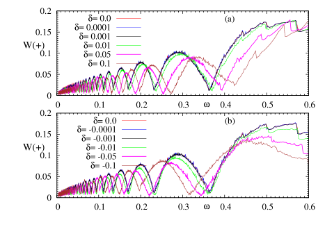
Figure 3: Plot shows the variation of EE for two channels with $(h+\delta)$ (in Fig. (a)) $(h-\delta)$ (in Fig. (b)) as a function of $\omega$. The minima of $W(-),~{}(W(+))$ shifts towards left (right) of the minima obtained for $W(\delta=0)$.

Using the properties of Bessel function and by retaining the leading order contribution in the limit $kT\ll 1$ and $\delta<1$, one can get

$$U_{k}^{{}^{\prime}}(\pm,t) \simeq I-i\biggl{[}{1\over 2}~{}(-k^{2}\pm 2\delta)\sigma_{z}+k\biggl{(}J_{0}\biggl{(}{2\over\omega}\biggr{)}$$

$$\mp {2\delta~{}T\over\pi}J_{1}\biggl{(}{2\over\omega}\biggr{)}\biggr{)}\sigma_{x}\mp 2kJ_{0}\biggl{(}{2\over\omega}\biggr{)}\delta~{}T~{}\sigma_{y}\biggr{]}T$$

$$\simeq I-i\biggl{[}{1\over 2}~{}(-k^{2}\pm 2\delta)\sigma_{z}+k\biggl{(}J_{0}\biggl{(}{2\over\omega}\biggr{)}$$

$$\mp {2\delta~{}T\over\pi}J_{1}\biggl{(}{2\over\omega}\biggr{)}\biggr{)}\sigma_{x}\biggr{]}T$$

$$\simeq I-iT\biggl{[}{1\over 2}(-k^{2}\pm 2\delta)\sigma_{z}+kJ_{0}\biggl{(}{2\pm 4\delta\over\omega}\biggr{)}\sigma_{x}\biggr{]}$$

Now, one can obtain the Floquet operator which is the time evolution operator in the initial frame $U_{k}(\pm,T)=R_{k}(\pm,T)U^{\prime}_{k}(\pm,T)R_{k}^{\dagger}(\pm,T)$ is given by

$$U_{k}(\pm,T)\simeq I-i\biggl{[}{1\over 2}~{}(-k^{2}\pm 2\delta)\sigma_{z}\mp 2k\delta TJ_{0}\biggl{(}{2\pm 4\delta\over\omega}\biggr{)}\sigma_{y}\biggr{]}T$$ (18)

One can therefore estimate the eigenstates (Floquet states) and eigen-energy (quasi-energy) by diagonalizing the Floquet operator (18). In the low frequency limit $k\ll J_{0}((2\pm 4\delta)/\omega)$, the behavior of $W(\pm)$ is determined by the behavior of Bessel function. In Fig. (4), we explicitly show that EE for the $(h(t)+\delta)$ channel the position of the minima of $W(+)$ matches with the zeros of the modified Bessel function $J_{0}((2+4\delta)/\omega)$. Therefore, the coupling to the qubit has an effect on the EE of the environmental spin chain.

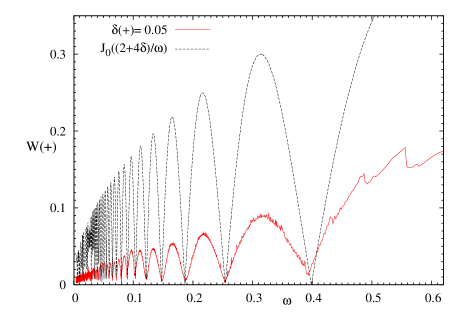
Figure 4: Plot shows the minima of EE for positive channel with $(h+\delta)$ are closely matching with the zeros of the Bessel’s function $J_{0}((2+4\delta)/\omega)$ while both of them are plotted as a function of $\omega$. Here, $\delta=0.05$.

Now, we focus on the response of EE in the intermediate frequency range where one observes a series of resonance peaks (see Fig. (5(a) and (b)). The position of this resonance peaks are also dependent on the channel of evolution and $\delta$. The resonance occurs when the quasi-degenerate momentum obtained from the energy spectrum associated with the Hamiltonian (5) crosses the edge of the BZ $k=\pi$. In oder to obtain the position of the peaks once again we have to take the limit $h_{0}\to 0$. Therefore, the resonance position can be determined from Eq. (15) and is given by

$$\omega_{r}(\pm)={4\mp 2\delta\over l},$$ (19)

where $l=1,2,3,\cdots$. According to this relation the shift of resonance frequency $\omega_{r}(\pm)$ from the uncoupled case when no qubit is coupled to the environmental chain is proportional to $\delta$. For example, the position of peaks for $\delta=0.05$ are $\omega_{r}(+)=3.9,~{}1.95,~{}1.3,~{}\cdots$ (see Fig. (5a)) which are successfully predicted by the Eq. (19). This resonance peaks are observed until the Bessel function starts dominating the low-frequency behavior of EE.

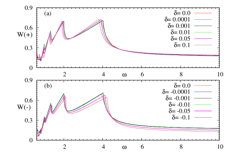
Figure 5: Plot shows the variation of EE for two channels with $(h+\delta)$ (in Fig. (a)) $(h-\delta)$ (in Fig. (b)) as a function of $\omega$. The peak of $W(-),~{}(W(+))$ shifts towards right (left) of the resonance peaks obtained for $W(\delta=0)$.

Now, we can investigate the high-frequency behavior of EE which shows a plateau like nature and the saturation value is again determined by the $\delta$ (see Fig. (6)). The high-frequency behavior is simply explained by taking into consideration the fact that the periodically varying transverse field vanishes on average. One can also use Magnus expansion to probe this limit blanes09 . Therefore, the effective environmental Hamiltonian in this high-frequency limit is given by

$${\cal H}^{\rm eff}_{k}(\pm)=(-1\pm\delta+\cos k)\sigma_{z}+\sin k\sigma_{x}$$ (20)

The effective quasi-energy when $\delta<1$ is given by $\mu^{\rm eff}_{k}(\pm)\simeq\pm 2(1\pm\delta/2)\sin(k/2)$. Therefore, one can naively conclude by continuing the analogy of effective quasi-energy to the EE that the deviation in EE from the uncoupled case is proportional to $\delta$ (see the inset of Fig. (6)). The EE for the positive channel saturates at a higher value than that of the negative channel.

One can exactly show that $W(\pm)=W(\delta=0)\pm O(\delta)$ in the high frequency limit where the dynamics of the system is governed by the critical Hamiltonian with $\delta$ (20). The quasi-states in this limit are given by $|\eta_{k}^{+}(\pm)\rangle=(\cos(\theta_{\pm}/2),~{}\sin(\theta_{\pm}/2))^{\cal T}$ and $|\eta_{k}^{-}(\pm)\rangle=(-\sin(\theta_{\pm}/2),~{}\cos(\theta_{\pm}/2))^{\cal T}$ where $\theta_{\pm}={\rm arctan}[\sin k/(-1\pm\delta+\cos k)]$ and ${\cal T}$ denotes the transpose of a matrix. The initial ground state wave-function can be written as $|\phi_{g,k}\rangle=(\cos(\theta_{g}/2),~{}\sin(\theta_{g}/2))^{\cal T}$ where $\theta_{g}={\rm arctan}[\sin k/(-2+\cos k)]$. $c_{k}^{+}(\pm)=\cos(\theta_{g}/2-\theta_{\pm}/2)$ and $c_{k}^{-}(\pm)=\sin(\theta_{g}/2-\theta_{\pm}/2)$. The work done for the two channels can be simplified to the following form

$$W(\pm) = (1/N)\sum_{k}\biggl{[}\biggl{(}\sin k\sin\theta_{\pm}+(-1\pm\delta+\cos k)\cos\theta_{\pm}\biggr{)}$$ (21)

$$\times \cos\biggl{(}\theta_{g}-\theta_{\pm}\biggr{)}+\sqrt{(2\pm\delta+\cos k)^{2}+\sin^{2}k}\biggr{]}$$

Now, one can expand the $\theta_{\pm}$ in the power series of $\delta$ with the constraint that $\delta<1$; $\theta_{\pm}=\theta_{0}\pm\delta({\partial\theta_{\pm}}/{\partial\delta})|_{\delta=0}+\cdots$. The difference between two Bogoliubov angles $\theta_{g}$ and $\theta_{\pm}$ is given by $\theta_{g}-\theta_{\pm}=\theta_{S}\mp\delta\theta_{D}$; $\theta_{S}=\theta_{g}-\theta_{0}$ and $\theta_{D}=({\partial\theta_{\pm}}/{\partial\delta})|_{\delta=0}$. We shall use the following assumption to obtain an approximated expression of $W(\pm)$ in the high frequency limit: $\cos(x+\delta y)=\cos x-\delta y\sin x$. The work done for two channels is then given by

$$W(\pm) =(1/N)\sum_{k}\biggl{[}\cos\theta_{S}\cos(k-\theta_{0})-\cos\theta_{S}\cos\theta_{0}$$ (22)

$$\pm {\delta\over 2}\biggl{(}2\cos\theta_{0}\cos\theta_{S}+4\theta_{D}\cos({k\over 2}+\theta_{S}-\theta_{0})$$

$$\times \sin{k\over 2}\biggr{)}+e_{g,k}(\delta=0)\pm\frac{\delta(2+\cos k)}{e_{g,k}(\delta=0)}\biggr{]}$$

$$= W(\delta=0)\pm O(\delta)$$

Therefore, we can see that the coupling to the qubit has an appreciable effect in EEs over all the three regions of frequency.

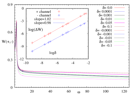
Figure 6: Plot shows the variation of EE for the both the channels with $(h\pm\delta)$ in the high $\omega$ limit. The saturation value is dependent on $\delta$. Inset shows that the amount of deviation in the saturation value of $W(\pm)$ from that of the bare EE $W(\delta=0)$ is linearly proportional to $\delta$.

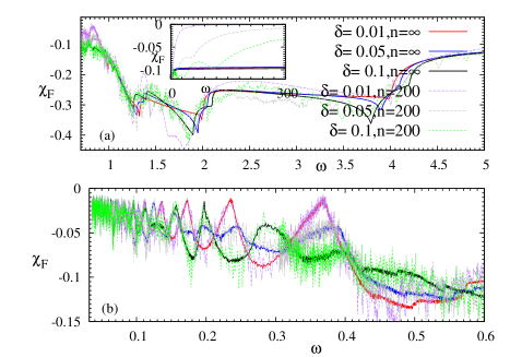
Figure 7: Plot shows the variation of DFSS $\chi_{F}$ for the finite $n$, obtained numerically, and infinite $n$, obtained analytically, as a function of $\omega$. The intermediate and low frequency behavior of $\chi_{F}$ are shown in Fig. (a) and Fig. (b), respectively. Fig. (a) shows that the intermediate frequency peak-dip structure is more prominently visible in $\chi_{F}(\infty)$ due to lack of oscillations. Inset of Fig. (a) shows that the high frequency saturation value of $\chi_{F}(n)$ is higher as compared to the $\chi_{F}(\infty)$. Fig. (b) depicts that the $\chi_{F}(n)$ is in very good agreement with the $\chi_{F}(\infty)$ in the low frequency regime.

We shall now focus on the behavior of DFSS as a function of frequency. We first present a comparative study between the two quantities $\chi_{F}(n)$ (12) obtained numerically for a large value of $n$ and $\chi_{F}(n\to\infty)$ (13) obtained analytically with frequency. In Fig.(7(a) and (b)), one can observe that the $\chi_{F}(\infty)$ is matching closely with $\chi_{F}(200)$ in intermediate and low frequency regime except the fact that DFSS for any finite $n$ oscillates rapidly around the mean curve designated by $\chi_{F}(\infty)$. In this low frequency regime, $\log(D_{k}^{\rm dec})$ is maximally contributing to the integral of $\chi_{F}(\infty)$ where as in the high frequency regime $x^{\prime}_{1}$ significantly contributes to the $\chi_{F}(\infty)$. The high frequency behavior of numerically obtained $\chi_{F}(n)$ is depicted in the inset of Fig. (7(a)) showing the deviation from the approximated expression of $\chi_{F}(\infty)$ (13) where “cross terms” $x^{\prime a}_{1}x^{\prime 2}_{m}$ (with $m\neq 1$) are neglected. Furthermore, in the intermediate frequency regime shown in Fig. (7(a)), the analytic expression $\chi_{F}(\infty)$ is sufficient to quantify the behavior of $\chi_{F}(n)$ as the “cross term” becomes very small; the decohered part and the $x^{\prime}_{m}$ part both contribute to the $\chi_{F}(\infty)$.

Now, we shall concentrate on the behavior of DFSS $\chi_{F}(\infty)$ as a function of frequency. We also present a comparative study between $\chi_{F}(\infty)$ and the EEs $W(\pm)$. Here as well we will study the $\chi_{F}(\infty)$ in three different frequency regimes. In Fig. (8(a)), we study the low-frequency characteristics of DFSS which qualitatively shows similar type of oscillations as observed in the case of $W(\pm)$. One can fully understand the behavior of $\chi_{F}(\infty)$ shown in Fig. (8(a)) by comparing the Fig. (8(b)) with the Fig. (8(c)). We can immediately conclude that the behavior of two channels of EEs actually determine the behavior of DFSS. We can see that when the oscillations for $W(+)$ coincides with that of the $W(-)$ we get nice oscillations in DFSS as an outcome of constructive superposition between the contribution coming from $|\phi_{k}(+)\rangle$ and $|\phi_{k}(-)\rangle$; this constructive interference occurs when the oscillations for $J_{0}((2+4\delta)/\omega)$ matches with that of the $J_{0}((2-4\delta)/\omega)$. On the other hand, DFSS also shows relatively flat regions as an effect of destructive interference between the two channels of the environmental wave-function. The interplay between two frequencies of oscillations leads to a beating like pattern of DFSS. Figure (8(a)) leads to the observation that the beating is more prominently visible for relatively higher values $\delta$. On the other hand, beating like pattern gradually turn into simple oscillatory behavior, governed by $J_{0}(2/\omega)$, as one decreases $\delta$.

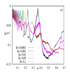
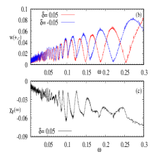
Figure 8: The behavior of $\chi_{F}(\infty)$ is strongly dependent on $\delta$ as shown in Fig. (a). Fig. (b) shows the variation of EE for the positive and negative channels with $(h\pm\delta)$ in the low $\omega$ limit. Fig. (c) depicts the response of $\chi_{F}(\infty)$ as a function of frequency.

In the intermediate frequency range, DFSS shows dip at the resonance frequency $\omega_{r}(\pm)$ (see Fig. (9)). The wave-functions for the two channels correspond to two different sets of $\omega_{r}$ where the resonance happens for that particular channel. As a consequence the DF being the modulus square overlap of the two wave-function evolving through two channels, $\Pi_{k}|\langle\phi_{k}(+)|\phi_{k}(-)\rangle|^{2}$, exhibits a change in its behavior at those $\omega_{r}(\pm)$; and this is reflected in the response of DFSS at this intermediate frequency range. The behavior of DFSS around $\omega_{r}(\pm)$ is more prominently visible for higher values of $\delta<1$. One can note that DFSS exhibits a dip at those resonance frequencies where $W(\pm)$ shows a peak. This is due to the fact that at those frequencies the wave-functions associated with the two channels become maximally deviated from each other.

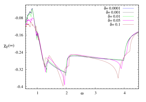
Figure 9: Plot shows that $\chi_{F}(\infty)$ exhibits a qualitatively similar behavior of that of the $W(\pm)$; although, the dip positions are dependent on $\delta$.

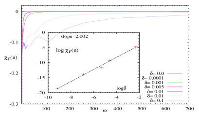
Figure 10: Plot shows high frequency saturation behavior of $\chi_{F}(n)$. Inset shows that saturation value of $\chi_{F}(n)$ is deviated by an amount $\delta^{2}$ from the bare $\chi_{F}(n)$ with coupling strength $\delta=0$.

At the end, we shall probe the high frequency behavior of DFSS. To observe the saturation value of DFSS, $\chi_{F}(\infty)$ is not an accurate quantity to be studied. This is due to the fact that high frequency saturation value of $\chi_{F}(\infty)$ does not tend towards zero when $\delta\to 0$ and vanishes for $\delta=0$. One can numerically check that in the high frequency regime, “cross term” $x^{\prime a}_{1}x^{\prime 2}_{m}$ with $m\neq 1$, contributes significantly to $\chi_{F}(\infty)$. This “cross term” gives an $O(\delta^{2})$ correction. Therefore, $\chi_{F}(\infty)$ (13) is not an accurate expression which can correctly describe the behavior of the high frequency saturation value of DFSS as a function of $\delta$. One can infer by observing Fig. (10) that the $\chi_{F}(n)$ is the appropriate quantity to examine the saturation behavior with $\delta$ in high frequency limit as the absolute value of $\chi_{F}(n)$ becomes smaller as one decreases $\delta$ and zero if $\delta=0$. Inset of Fig. (10) shows that the saturation value is proportional to $\delta^{2}$. This observation of vanishing $\chi_{F}(n)$ can be justified by analyzing the Eq.(12) with a comparative study between the decohered value $D_{k}^{\rm dec}$ and the $T^{\prime}_{m}$ terms. One can see that $\delta=0$ leads to the following fact: $D^{\rm dec}_{k}$ and the cross terms consisting of $x_{m}\cos\alpha_{m}$’s sum up to unity for each momentum mode while $n$ has a finite value; $\cos\alpha_{m}=1$ as $\delta=0$. This leads to the observation of a vanishing DFSS $\chi_{F}(\delta=0,n)$ in all frequencies. Therefore, we can infer that $\chi_{F}(\infty)$ follows the behavior of $\chi_{F}(n)$ in all the other frequency regimes except in the high frequency regime.

We shall now concentrate on the functional behavior of $\delta$ over the high frequency saturation value of DFSS as shown in Fig. (10). As we mention previously for the case of EEs, one can get a qualitatively approximate expression of the quasi-states and the quasi-energies by diagonalizing the effective Hamiltonian in Eq. (20). We can therefore define an effective expression of the DF, qualitatively valid only for infinite frequency regime, in the momentum space is given by

$$D^{\rm eff}_{k} = |\langle\eta_{k}(+)|\eta_{k}(-)\rangle|^{2}=\cos^{2}\biggl{(}{\theta_{+}-\theta_{-}\over 2}\biggr{)}$$ (23)

$$\simeq 1-{\delta^{2}\over 4}\sin^{2}{k\over 2}$$

DF is $D^{\rm eff}=\Pi_{k>0}D^{\rm eff}_{k}$. This over simplified expression of $D^{\rm eff}_{k}$ is not a quantitatively accurate expression because it does not give the high frequency saturation value of DFSS $\chi_{F}(n)$ correctly. We can only infer from the above expression that the infinite frequency saturation value of DFSS (12) of the qubit $\chi_{F}(n)$ is deviated from that of the $\chi_{F}(n,\delta=0)$ by an amount proportional to $\delta^{2}$.

One can also use the usual definition of fidelity susceptibility zanardi06 $\chi_{F}(n)=\log(D(n))/N=\delta^{2}\chi_{\cal F}(n)$ to probe its high frequency saturation behavior where $\chi_{\cal F}(n)$ in our case is given by

$$\chi_{\cal F}(n) = \biggl{[}\left\langle\frac{\partial}{\partial\delta}\phi_{k}(+,nT)\left|\frac{\partial}{\partial\delta}\phi_{k}(-,nT)\right.\right\rangle$$ (24)

$$-\left\langle\left.\frac{\partial}{\partial\delta}\phi_{k}(+,nT)\right|\phi_{k}(-,nT)\right\rangle$$

$$\left\langle\phi_{k}(+,nT)\left|\frac{\partial}{\partial\delta}\phi_{k}(-,nT)\right.\right\rangle\biggr{]}_{\delta=0}.$$

Therefore, it is evident from the above Eq. (24) that the $\chi_{F}(n)\propto\delta^{2}$ as $\chi_{\cal F}(n)$ is independent of $\delta$. We can see that in all the frequency regime the EE and DFSS are modified by the small parameter $\delta$ and their behavior are connected to each other through this small parameter $\delta$.

IV conclusion

In conclusion, we choose a central spin model where a single qubit is globally coupled to an environmental Ising spin chain periodically driven across its QCP and numerically study the EE associated with it as a function of frequency in the infinite time limit; we also numerically investigate the DFSS of the qubit after a large number of period with frequency. Our aim is to characterize the behavior of EE and DFSS when a small system-environment coupling parameter is present and analyze their behavior by plausible analytical argument. The coupling to the qubit gives rise to two channels of time evolution for the environment and consequently leads to two separate species of Floquet operators. In the process, we show that the coupling strength $\delta$ can influence the position of quasi-degenerate momentum mode in the Floquet spectrum associated with the two species of Floquet operators. We have two sets of EEs $W(\pm)$ each of them is associated with the one of these channels. We show that the low-frequency oscillations of $W(\pm)$ for two channels are dominated by the two different Bessel functions with argument dependent on $\delta$. The position of the resonance peaks at intermediate frequencies for two channels are different from each other due to the finite coupling strength. Finally, high frequency saturation value of EEs for two channels are dependent on $\delta$ in such a way that the EE for the positive channel takes a higher value of saturation than that of the negative channel.

In parallel, we find an analytical expression for the $\chi_{F}(n\to\infty)$ which can successfully predict the behavior of the DFSS $\chi_{F}(n)$, obtained numerically for a large value of $n$, in the low and intermediate frequency regime. We show that the behavior of DFSS of the qubit $\chi_{F}(\infty)$ in the above frequency regions can be speculated by understanding the behavior of EEs for the two channels of evolution associated with environmental spin chain. DFSS exhibits low-frequency beating like pattern originated from the interplay between two Bessel functions, governing the oscillations of $W(\pm)$, with two different arguments. $\chi_{F}(\infty)$ displays dips at intermediate frequencies where the $W(\pm)$ show peaks. The position of these dips, appearing due to destructive interference between two channels of environment, are dependent on $\delta$. At the end, the DFSS tends to saturation value at high frequency which is correctly quantified by $\chi_{F}(n)$ instead of $\chi_{F}(\infty)$. The saturation value of $\chi_{F}(n)$ is deviated from the bare saturation value of DFSS $\chi_{F}(n,\delta=0)=0$ by an amount proportional to $\delta^{2}$. This deviation of $O(\delta^{2})$ can be estimated from the effective DFSS defined for the high frequency static Hamiltonian which also successfully predicts the correction of $O(\delta)$ in EE at the high frequency limit. Therefore, in all the above three frequency region the behavior of DFSS is closely tied with the behavior of EEs for two different channels.

Moreover, the Loschmidt echo has been experimentally investigated in an antiferromagnetic Ising spin chain with finite number of spins using NMR quantum simulator zhang09 . The periodic driving has also been experienced experimentally leading to many interesting observations kitagawa12 . Therefore, experimental verification of our work might be possible by employing a time periodic model in the large scale NMR quantum simulator.

V Acknowledgements

The author acknowledges Amit Dutta for critically reading the manuscript and giving useful suggestions. The author also thanks Victor Mukherjee for valuable discussions.

Appendix A Exact Calculation of $\chi_{F}(\infty)$

In this appendix, we shall explicitly calculate the DFSS $\chi_{F}(\infty,\delta)$ (13) in the $n\to\infty$ limit with $\delta<1$. We shall calculate each term of $D(n)$ including $T_{m}$’s and show their functional dependence on $\delta$. The quasi-state $|\eta_{k}^{\pm}(\pm)\rangle$, associated with the two species of Floquet operators ${\cal F}_{k}(\pm)$, can be expanded in the powers of $\delta$

$$|\eta^{\pm}_{k}(\pm)\rangle=|\eta^{\pm}_{k}(0)\rangle\pm\delta~{}\frac{\partial|\eta_{k}^{\pm}(\pm)\rangle}{\partial\delta}|_{\delta=0}+\cdots,$$ (25)

where $|\eta^{\pm}_{k}(0)\rangle$ is the quasi-state of bare Floquet operator ${\cal F}_{k}(\delta=0)$. Now, one can easily calculate the the Floquet coefficients $c^{\pm}_{k}(\pm)$ in the power series of $\delta$

$$c^{\pm}_{k}(\pm)=c^{\pm}_{k}(0)\pm\delta~{}\frac{\partial c_{k}^{\pm}(\pm)}{\partial\delta}|_{\delta=0}+\cdots.$$ (26)

Here, $({\partial c_{k}^{\pm}(\pm)}/{\partial\delta})=\langle\phi_{g,k}|{\partial|\eta_{k}^{\pm}(\pm)\rangle}/{\partial\delta}$. Similarly, the overlap $\langle\eta^{\pm}_{k}(+)|\eta^{\pm}_{k}(-)\rangle$ can also be expanded in the ascending powers of $\delta$. Now, $\langle\eta^{\pm}_{k}(+)|\eta^{\pm}_{k}(-)\rangle$ is given by

$$\langle\eta^{\pm}_{k}(+)|\eta^{\pm}_{k}(-)\rangle=1-\delta^{2}~{}\biggl{[}\frac{\partial\langle\eta^{\pm}_{k}(+)|\partial|\eta^{\pm}_{k}(-)\rangle}{\partial\delta}\biggr{]}_{\delta=0}$$ (27)

On the other hand, $\langle\eta^{\pm}_{k}(+)|\eta^{\mp}_{k}(-)\rangle$ is given by

$$\langle\eta^{\pm}_{k}(+)|\eta^{\mp}_{k}(-)\rangle = -\delta~{}\biggl{[}\frac{\langle\eta^{\pm}_{k}(0)|\partial|\eta^{\mp}_{k}(-)\rangle}{\partial\delta}\biggr{]}_{\delta=0}$$

$$+ \delta\biggl{[}\frac{\partial\langle\eta^{\pm}_{k}(+)|\eta^{\mp}_{k}(0)\rangle}{\partial\delta}\biggr{]}_{\delta=0}+O(\delta^{2})$$

Now, we shall analyze each term of $D(n)$ and its dependence on $\delta$.

$$|c_{k}^{+}(+)|^{2}|c_{k}^{+}(-)|^{2}~{}|\langle\eta_{k}^{+}(+)|\eta_{k}^{+}(-)\rangle|^{2}\to|c_{k}^{+}(0)|^{4}+O(\delta^{2})$$

$$|c_{k}^{-}(+)|^{2}|c_{k}^{-}(-)|^{2}~{}|\langle\eta_{k}^{-}(+)|\eta_{k}^{-}(-)\rangle|^{2}\to|c_{k}^{-}(0)|^{4}+O(\delta^{2})$$

$$|c_{k}^{+}(+)|^{2}|c_{k}^{-}(-)|^{2}|\langle\eta_{k}^{+}(+)|\eta_{k}^{-}(-)\rangle|^{2}\to O(\delta^{2})$$

$$|c_{k}^{-}(+)|^{2}|c_{k}^{+}(-)|^{2}|\langle\eta_{k}^{-}(+)|\eta_{k}^{+}(-)\rangle|^{2}\to O(\delta^{2})$$

$$T^{\prime}_{1}\to|c_{k}^{+}(0)|^{2}|c_{k}^{-}(0)|^{2}+O(\delta^{2}),~{}T^{\prime}_{2}\to O(\delta)$$

$$T^{\prime}_{3}\to O(\delta),~{}T^{\prime}_{4}\to O(\delta),T^{\prime}_{5}\to O(\delta),~{}T^{\prime}_{6}\to O(\delta^{2})$$

One can probe the $\delta$-dependence on the $x^{\prime}_{m}$ using the above observation. This leads to the following fact $x^{\prime}_{1}\to O(\delta^{0})+O(\delta^{2})+O(\delta^{4})$, $x^{\prime}_{m}\to O(\delta)+O(\delta^{3})$ with $m=2,3,4,~{}5$ and $x^{\prime}_{6}\to O(\delta^{2})+O(\delta^{4})$.

Therefore, one can write an approximated expression of $\chi_{F}(n\to\infty)$ by a momentum space integration over the $x^{\prime}_{m}\cos\alpha_{m}$. In order to estimate $\chi_{F}(n\to\infty)$, we define a quantity $A$ which is given by

$$A =\log\biggl{[}1+\sum_{m=1}^{6}z_{m}\biggr{]}$$ (28)

$$= \sum_{m}z_{m}-{1\over 2}\sum_{m,n}z_{m}z_{n}+{1\over 3}\sum_{m,n,p}z_{m}z_{n}z_{p}+\cdots$$

$\chi_{F}(n)$ is then given by $\chi_{F}(n)={1\over N}\sum_{k}[\log(D_{k}^{\rm dec})+A]$. Here, $z_{m}={x^{\prime}_{m}}\cos\alpha_{m}$. $x^{\prime}_{m}$ and $\alpha_{m}$ are $k$ dependent functions.

One can obtain the following type of terms by decomposing the above Eq. (28).

$$z_{i} = \sum_{i}x^{\prime}_{i}\cos\alpha_{i},~{}z_{i}z_{j}=\sum_{i,j}x^{\prime}_{i}x^{\prime}_{j}\cos\alpha_{i}\cos\alpha_{j}$$

$$= {1\over 2}\sum_{i,j}x^{\prime}_{i}x^{\prime}_{j}\biggl{(}\cos(\alpha_{i}+\alpha_{j})+\cos(\alpha_{i}-\alpha_{j})\biggr{)},~{}$$

$$z_{i}z_{j}z_{k} = \sum_{i,j,k}x^{\prime}_{i}x^{\prime}_{j}x^{\prime}_{k}\cos\alpha_{i}\cos\alpha_{j}\cos\alpha_{k}$$

$$= {1\over 4}\sum_{i,j,k}x^{\prime}_{i}x^{\prime}_{j}x^{\prime}_{k}\biggl{(}\cos(\alpha_{i}+\alpha_{j}+\alpha_{k})+\cos(\alpha_{i}+\alpha_{j}-\alpha_{k})$$

$$+ \cos(\alpha_{i}-\alpha_{j}+\alpha_{k})+\cos(\alpha_{i}-\alpha_{j}-\alpha_{k})\biggr{)}$$

$$z_{i}z_{j}z_{k}z_{l} = \sum_{i,j,k,l}x^{\prime}_{i}x^{\prime}_{j}x^{\prime}_{k}x^{\prime}_{l}\cos\alpha_{i}\cos\alpha_{j}\cos\alpha_{k}\cos\alpha_{l}$$

$$= {1\over 8}\sum_{i,j,k,l}x^{\prime}_{i}x^{\prime}_{j}x^{\prime}_{k}x^{\prime}_{l}\biggl{(}\cos(\alpha_{i}+\alpha_{j}+\alpha_{k}+\alpha_{l})$$

$$+ \cos(\alpha_{i}-\alpha_{j}+\alpha_{k}+\alpha_{l})+\cos(\alpha_{i}+\alpha_{j}-\alpha_{k}+\alpha_{l})$$

$$+ \cos(\alpha_{i}-\alpha_{j}-\alpha_{k}+\alpha_{l})+\cos(\alpha_{i}+\alpha_{j}+\alpha_{k}-\alpha_{l})$$

$$+ \cos(\alpha_{i}-\alpha_{j}+\alpha_{k}-\alpha_{l})+\cos(\alpha_{i}+\alpha_{j}-\alpha_{k}-\alpha_{l})$$

$$+ \cos(\alpha_{i}-\alpha_{j}-\alpha_{k}-\alpha_{l})\biggr{)}$$

Here, $\alpha_{i}$ is a function of $\mu^{\pm}_{k}(\pm)nT$. As $n\to\infty$, the complete momentum integration over the power series of $z_{i}$ gives non-zero values when the argument of the cosine term vanishes. Now, the argument of the cosine term vanishes only when an even number of sum is involved inside the argument with alternating signs but the same index. For example, the integration over $z_{i}z_{j}$ yields $\sum_{i}x^{\prime 2}_{i}/2$ as $\cos(\alpha_{i}+\alpha_{j})$ does not survive under integration while $\cos(\alpha_{i}-\alpha_{j})$ survives only for $i=j$. Similarly, integration over $z_{i}z_{j}z_{k}z_{l}$ and $z_{i}z_{j}z_{k}z_{l}z_{m}z_{n}$ contribute $\sum_{i}3x^{\prime 4}_{i}/8$ and $\sum_{i}5x^{\prime 6}_{i}/16$ to the $\chi_{F}(\infty)$, respectively.

One can see that $\chi_{F}(\infty)$ receives a contribution of $O(\delta^{0})$ with $O(\delta^{2})$ from the decohered part. Now, for $m\neq 1$ and $m\neq 6$ the leading order term from the non-decohered part, coming from $x^{\prime 2}_{m}$, is $O(\delta^{2})$. The next leading order term of $O(\delta^{4})$ is therefore coming from $x^{\prime 4}_{m}$; $x^{\prime n}_{m}\to O(\delta^{n})$. For $m=6$, $x^{\prime n}_{6}\to O(\delta^{2n})$. In the case of $m=1$, the $x^{\prime 2p}_{1}$ ($p$ is an integer) generates all even power terms in $\delta$ starting from $O(\delta^{0})$ to $O(\delta^{2p})$. Therefore, in order to incorporate the complete $O(\delta^{0})$ contribution, one has to consider the full series consisting the even powers in $x^{\prime}_{1}$; this results in the closed form expression $\log(2/(1+\sqrt{1-x^{\prime 2}_{1}}))$. The others power series can be safely truncated by retaining only the leading contributions. One can exclude $x^{\prime 2}_{6}$ term as it has $O(\delta^{4})$ correction.

Here, one can also get a finite contribution from even order term like $x^{\prime 2p}_{i}x^{\prime 2q}_{j}$, referred as the “cross term” in Eq. (13), with $i\neq j$, $p$ and $q$ can be any positive integer. This type of terms appear when the argument of the cosine term vanishes in a pair. For example, $z_{i}z_{j}z_{k}z_{l}$ yields $x^{\prime 2}_{i}x^{\prime 2}_{j}$ type of terms from the momentum integration over $\cos(\alpha_{i}-\alpha_{l}+\alpha_{j}-\alpha_{k})$ with $i=l$ and $j=k$. This type of fourth order terms are the lowest order term from which the series of $x^{\prime 2p}_{i}x^{\prime 2q}_{j}$ starts contributing to the momentum integral of $\chi_{F}(n\to\infty)$. But, the contribution coming from this term is $O(\delta^{4})$ except the product terms like $x^{\prime 2p}_{1}x^{\prime 2}_{m}$ (with $m\neq 1,6$) which has an $O(\delta^{2})$ correction. A closed form expression can not be obtained for this $O(\delta^{2})$ terms. Numerical investigation suggests that the product $x^{\prime}_{1}x^{\prime}_{m}$ becomes insignificantly small in low and intermediate frequency. Therefore, one can neglect the above $O(\delta^{2})$ contribution in low and intermediate frequency regime; $\chi_{F}(\infty)$ can be constructed by keeping only the leading order contribution coming from the decohered part and $x^{\prime 2p}_{m}$ (with $m=1,~{}\cdots,~{}6$) part. Combining all the significant contribution one can write the approximated of $\chi_{F}(\infty)$ (13) in low and intermediate frequency regime.

References

- (1)
- (2) W. H. Zurek, U. Dorner, and P. Zoller, Phys. Rev. Lett. 95, 105701 (2005).
- (3) A. Polkovnikov, Phys. Rev. B 72, 161201(R) (2005).
- (4) B. Damski, Phys. Rev. Lett. 95, 035701 (2005); J. Dziarmaga, Phys. Rev. Lett. 95, 245701 (2005); R. W. Cherng and L. S. Levitov, Phys. Rev. A 73, 043614 (2006).
- (5) V. Mukherjee, U. Divakaran, A.Dutta and D. Sen, Phys. Rev. B 76, 174303 (2007).
- (6) V. Mukherjee and A. Dutta, J. Stat. Mech. (2009) P05005.
- (7) J. Dziarmaga, Adv. Phys. 59, 1063 (2010).
- (8) A. Polkovnikov, K. Sengupta, A. Silva, and M. Vengalattore, Rev.Mod.Phys. 83, 863 (2011).
- (9) R. Barankov and A. Polkovnikov, Phys. Rev. Lett. 101, 076801.
- (10) K. Sengupta and D. Sen, Phys. Rev. A 80, 032304 (2009).
- (11) H. T. Quan, W. H. Zurek, New Journal of Physics 12 (2010) 093025.
- (12) T. Nag, A. Patra and A. Dutta, Jour. Stat. Mech. (2011) P08026.
- (13) T. Nag, A. Dutta and A. Patra, Int. J. Mod. Phys. B 27, 1345036, (2013).
- (14) V. Mukherjee, S. Sharma and A. Dutta, Rev. B, 86 020301 (R) (2012).
- (15) S. Suzuki, T. Nag and A. Dutta, arXiv: 1509.04649.
- (16) J. H. Shirley, Phys. Rev. 138, B979 (1965).
- (17) F. Grossmann, T. Dittrich, P. Jung, and P. Hänggi, Phys. Rev. Lett. 67, 516 (1991); F. Grossmann and P. Hänggi, Eur. Phys. Lett. 18, 571 (1992).
- (18) M. Grifoni amd P. Hänggi, Physics Reports 304, 229 (1998).
- (19) Y. Kayanuma, Phys. Rev. A, 50 (1994) 843.
- (20) E. Canovi, D. Rossini, R. Fazio, G. E. Santoro, and A. Silva, New J. Phys. 14, 095020 (2012).
- (21) A. Russomanno, A. Silva, and G. E. Santoro, Phys. Rev. Lett. 109, 257201 (2012).
- (22) A. Das, Phys. Rev. B 82, 172402 (2010); S. Bhattacharyya, A. Das, and S. Dasgupta, Phys. Rev. B 86, 054410 (2012).
- (23) V. M. Bastidas, C. Emary, G. Schaller and T. Brandes Phys. Rev. A 86, 063627 (2012); G. Engelhardt, V. M. Bastidas, C. Emary, T. Brandes, Phys. Rev. E 87, 052110 (2013); S. Dasgupta, U. Bhattacharya, and A. Dutta, Phys. Rev. E 91, 052129 (2015).
- (24) A. Russomanno , A. Silva A.and G. E. Santoro, J. Stat. Mech., (2013) P09012.
- (25) A. Lazarides, A. Das, and R. Moessner, Phys. Rev. Lett. 112, 150401 (2014).
- (26) T. Nag, S. Roy, A. Dutta, and D. Sen, Phys. Rev. B 89 165425 (2014).
- (27) T. Nag, D. Sen and A. Dutta, Phys. Rev. A 91, 063607 (2015).
- (28) Z. Gu, H. A. Fertig, D. P. Arovas, and A. Auerbach, Phys. Rev. Lett. 107, 216601 (2011).
- (29) T. Kitagawa, T. Oka, A. Brataas, L. Fu, and E. Demler, Phys. Rev. B 84, 235108 (2011).
- (30) A. Gomez-Leon and G. Platero, Phys. Rev. B 86, 115318 (2012), and Phys. Rev. Lett. 110, 200403 (2013); B. Dóra, J. Cayssol, F. Simon, and R. Moessner, Phys. Rev. Lett. 108, 056602 (2012); J. Cayssol, B. Dora, F. Simon, and R. Moessner, Phys. Status Solidi RRL 7, 101 (2013); D. E. Liu, A. Levchenko, and H. U. Baranger, Phys. Rev. Lett. 111, 047002 (2013); Q.-J. Tong, J.-H. An, J. Gong, H.-G. Luo, and C. H. Oh, Phys. Rev. B 87, 201109(R) (2013).
- (31) T. Kitagawa, M. A. Broome, A. Fedrizzi, M. S. Rudner, E. Berg, I. Kassal, A. Aspuru-Guzik, E. Demler, and A. G. White, Nat. Commun. 3, 882 (2012); M. C. Rechtsman, J. M. Zeuner, Y. Plotnik, Y. Lumer, D. Podolsky, S. Nolte, F. Dreisow, M. Segev, and A. Szameit, Nature 496, 196 (2013); M. C. Rechtsman, Y. Plotnik, J. M. Zeuner, D. Song, Z. Chen, A. Szameit, and M. Segev, Phys. Rev. Lett. 111, 103901 (2013).
- (32) A. Russomanno, S. Sharma, A. Dutta and G. E. Santoro, Jour. Stat. Mech. (2015) P08030.
- (33) M. A. Nielsen and I. L. Chuang,Quantum Computation and Quantum Information (Cambridge University Press, Cambridge, UK, 2000).
- (34) V. Vedral, Introduction to Quantum Information Science (Oxford University Press, Oxford, UK, 2007).
- (35) B. K. Chakrabarti, A. Dutta, and P. Sen, Quantum Ising Phases and transitions in transverse Ising Models, m41 (Springer, Heidelberg, 1996).
- (36) S. Sachdev, Quantum Phase Transitions(Cambridge University Press, Cambridge, England,1999).
- (37) A. Dutta, G. Aeppli, B. K. Chakrabarti, U. Divakaran, T. Rosenbaum and D. Sen, Quantum Phase Transitions in Transverse Field Spin Models: From Statistical Physics to Quantum Information (Cambridge University Press, Cambridge, 2015).
- (38) W. H. Zurek, Rev. Mod. Phys. 75, 715 (2003); E. Joos, H. D. Zeh, C. Keifer, D. Giulliani, J. Kupsch and I. -O. Stamatescu, Decoherence and appearance of a classical world in a quantum theory, (Springer Press, Berlin) (2003).
- (39) H. T. Quan, Z. Song, X. F. Liu, P. Zanardi, and C. P. Sun, Phys. Rev. Lett. 96, 140604 (2006).
- (40) B. Damski, H. T. Quan, W. H. Zurek, Phys. Rev. A 83, 062104 (2011).
- (41) T. Nag, U. Divakaran and A. dutta, Phys. Rev. B, 86 020401 (R) (2012).
- (42) S. Roy, T. Nag and A. Dutta, EPJ B 86, 204 (2013).
- (43) R. Sachdeva, T. Nag, A. Agarwal and A. Dutta, Phys. Rev. B 90, 045421 (2014).
- (44) John Schliemann, Alexander V. Khaetskii, and Daniel Loss, Phys. Rev. B 66, 245303 (2002).
- (45) F. M. Cucchietti, , Phys. Rev. A 75, 032337 (2007); D. Rossini, , Phys. Rev. A 75, 032333 (2007); J. Zhang, , Phys. Rev. A 79, 012305 (2009).
- (46) Lorenzo C Venuti and P. Zanardi, Phys. Rev. A 81, 022113 (2010); Lorenzo C Venuti, , Phys. Rev. Lett. 107, 010403 (2011).
- (47) S. Sharma, A. Russomanno, G. E. Santoro, and A. Dutta, EPL 106, 67003 (2014)
- (48) J. Zhang, F. M. Cucchietti, C. M. Chandrashekar, M. Laforest, C. A. Ryan, M. Ditty, A. Hubbard, J. K. Gamble, and R. Laflamme, Phys. Rev. A 79, 012305 (2009).
- (49) J.E. Bunder and R. H. McKenzie, Phys. Rev. B., 60, 344, (1999).
- (50) E. Lieb, T. Schultz and D. Mattis, Annals of Physics, 16, 407 (1961).
- (51) P. Zanardi and N. Paunkovic, Phys. Rev. E 74, 031123 (2006), H. Zhou and J. P. Barjaktarevic, J. Phys. A, 41 412001 (2008), C. De Grandi, V. Gritsev, and A. Polkovnikov, Phys. Rev. B 81, 012303 (2010), S.-J. Gu, Int. J. Mod. Phys B 24, 4371 (2010).
- (52) S. Blanes, F. Casas, J. A. Oteo, and J. Ros, Phys. Rep. 470, 151 (2009).