An Extension of Möbius–Lie Geometry
with Conformal Ensembles of Cycles
and Its Implementation in a GiNaC Library

Abstract.

We propose to consider ensembles of cycles (quadrics), which are interconnected through conformal-invariant geometric relations (e.g. “to be orthogonal”, “to be tangent”, etc.), as new objects in an extended Möbius–Lie geometry. It was recently demonstrated in several related papers, that such ensembles of cycles naturally parameterise many other conformally-invariant objects, e.g. loxodromes or continued fractions.

The paper describes a method, which reduces a collection of conformally invariant geometric relations to a system of linear equations, which may be accompanied by one fixed quadratic relation. To show its usefulness, the method is implemented as a C++ library. It operates with numeric and symbolic data of cycles in spaces of arbitrary dimensionality and metrics with any signatures. Numeric calculations can be done in exact or approximate arithmetic. In the two- and three-dimensional cases illustrations and animations can be produced. An interactive Python wrapper of the library is provided as well.

1. Introduction

Lie sphere geometry  [Cecil08a] [Benz07a]*Ch. 3 in the simplest planar setup unifies circles, lines and points—all together called cycles in this setup. Symmetries of Lie spheres geometry include (but are not limited to) fractional linear transformations (FLT) of the form:

(1) $$\begin{pmatrix}a&b\\ c&d\end{pmatrix}:\ x\mapsto\frac{ax+b}{cx+d}\,,\qquad\text{where }\det\begin{pmatrix}a&b\\ c&d\end{pmatrix}\neq 0.$$

Following other sources, e.g.  [Simon11a]*§ 9.2, we call (1) by FLT and reserve the name “Möbius maps” for the subgroup of FLT which fixes a particular cycle. For example, on the complex plane FLT are generated by elements of $\mathrm{SL}_{2}(\mathbb{C}{})$ and Möbius maps fixing the real line are produced by $\mathrm{SL}_{2}(\mathbb{R}{})$ [Kisil12a]*Ch. 1.

There is a natural set of FLT-invariant geometric relations between cycles (to be orthogonal, to be tangent, etc.) and the restriction of Lie sphere geometry to invariants of FLT is called Möbius–Lie geometry. Thus, an ensemble of cycles, structured by a set of such relations, will be mapped by FLT to another ensemble with the same structure.

It was shown recently that ensembles of cycles with certain FLT-invariant relations provide helpful parametrisations of new objects, e.g. points of the Poincaré extended space [Kisil15a], loxodromes [KisilReid18a] or continued fractions [BeardonShort14a, Kisil14a], see Example 3 below for further details. Thus, we propose to extend Möbius–Lie geometry and consider ensembles of cycles as its new objects, cf. formal Defn. 5. Naturally, “old” objects—cycles—are represented by simplest one-element ensembles without any relation. This paper provides conceptual foundations of such extension and demonstrates its practical implementation as a C++ library figure. Interestingly, the development of this library shaped the general approach, which leads to specific realisations in [Kisil15a, Kisil14a, KisilReid18a].

More specifically, the library figure manipulates ensembles of cycles (quadrics) interrelated by certain FLT-invariant geometric conditions. The code is build on top of the previous library cycle [Kisil05b, Kisil12a, Kisil06a], which manipulates individual cycles within the GiNaC [GiNaC] computer algebra system. Thinking an ensemble as a graph, one can say that the library cycle deals with individual vertices (cycles), while figure considers edges (relations between pairs of cycles) and the whole graph. Intuitively, an interaction with the library figure reminds compass-and-straightedge constructions, where new lines or circles are added to a drawing one-by-one through relations to already presented objects (the line through two points, the intersection point or the circle with given centre and a point). See Example 6 of such interactive construction from the Python wrapper, which provides an analytic proof of a simple geometric statement.

It is important that both libraries are capable to work in spaces of any dimensionality and metrics with an arbitrary signatures: Euclidean, Minkowski and even degenerate. Parameters of objects can be symbolic or numeric, the latter admit calculations with exact or approximate arithmetic. Drawing routines work with any (elliptic, parabolic or hyperbolic) metric in two dimensions and the euclidean metric in three dimensions.

The mathematical formalism employed in the library cycle is based on Clifford algebras, which are intimately connected to fundamental geometrical and physical objects [HestenesSobczyk84a, Hestenes15a]. Thus, it is not surprising that Clifford algebras have been already used in various geometric algorithms for a long time, for example see [Hildenbrand13a, Vince08a, DorstDoranLasenby02a] and further references there. Our package deals with cycles through Fillmore–Springer–Cnops construction (FSCc) which also has a long history, see [Schwerdtfeger79a]*§ 1.1 [Cnops02a]*§ 4.1 [FillmoreSpringer90a] [Kirillov06]*§ 4.2 [Kisil05a] [Kisil12a]*§ 4.2 and section 2.1 below. Compared to a plain analytical treatment [Pedoe95a]*Ch. 2 [Benz07a]*Ch. 3, FSCc is much more efficient and conceptually coherent in dealing with FLT-invariant properties of cycles. Correspondingly, the computer code based on FSCc is easy to write and maintain.

The paper outline is as follows. In Section 2 we sketch the mathematical theory (Möbius–Lie geometry) covered by the package of the previous library cycle [Kisil05b] and the present library figure. We expose the subject with some references to its history since this can facilitate further development.

Sec. 3.1 describes the principal mathematical tool used by the library figure. It allows to reduce a collection of various linear and quadratic equations (expressing geometrical relations like orthogonality and tangency) to a set of linear equations and at most one quadratic relation (8). Notably, the quadratic relation is the same in all cases, which greatly simplifies its handling. This approach is the cornerstone of the library effectiveness both in symbolic and numerical computations. In Sec. 3.2 we present several examples of ensembles, which were already used in mathematical theories [Kisil15a, Kisil14a, KisilReid18a], then we describe how ensembles are encoded in the present library figure through the functional programming framework.

Sec. 4 outlines several typical usages of the package. An example of a new statement discovered and demonstrated by the package is given in Thm. 7. In Sec. 5 we list of some further tasks, which will extend capacities and usability of the package.

All coding-related material is enclosed as appendices. App. A contains examples of the library usage starting from the very simple ones. A systematic list of callable methods is given in Apps LABEL:sec:publ-meth-figure–LABEL:sec:addtional-utilities. Any of Sec. 2 or Apps A–LABEL:sec:publ-meth-figure can serve as an entry point for a reader with respective preferences and background. Actual code of the library is collected in Apps LABEL:sec:figure-header-file–LABEL:sec:impl-class.

2. Möbius–Lie Geometry and the cycle Library

We briefly outline mathematical formalism of the extend Möbius–Lie geometry, which is implemented in the present package. We do not aim to present the complete theory here, instead we provide a minimal description with a sufficient amount of references to further sources. The hierarchical structure of the theory naturally splits the package into two components: the routines handling individual cycles (the library cycle briefly reviewed in this section), which were already introduced elsewhere [Kisil05b], and the new component implemented in this work, which handles families of interrelated cycles (the library figure introduced in the next section).

2.1. Möbius–Lie geometry and FSC construction

Möbius–Lie geometry in $\mathbb{R}^{n}{}$ starts from an observation that points can be treated as spheres of zero radius and planes are the limiting case of spheres with radii diverging to infinity. Oriented spheres, planes and points are called together cycles. Then, the second crucial step is to treat cycles not as subsets of $\mathbb{R}^{n}{}$ but rather as points of some projective space of higher dimensionality, see [Benz08a]*Ch. 3 [Cecil08a] [Pedoe95a] [Schwerdtfeger79a].

To distinguish two spaces we will call $\mathbb{R}^{n}{}$ as the point space and the higher dimension space, where cycles are represented by points—the cycle space. Next important observation is that geometrical relations between cycles as subsets of the point space can be expressed in term of some indefinite metric on the cycle space. Therefore, if an indefinite metric shall be considered anyway, there is no reason to be limited to spheres in Euclidean space $\mathbb{R}^{n}{}$ only. The same approach shall be adopted for quadrics in spaces $\mathbb{R}^{pqr}{}$ of an arbitrary signature $p+q+r=n$, including $r$ nilpotent elements, cf. (2) below.

A useful addition to Möbius–Lie geometry is provided by the Fillmore–Springer–Cnops construction (FSCc) [Schwerdtfeger79a]*§ 1.1 [Cnops02a]*§ 4.1 [Porteous95]*§ 18 [FillmoreSpringer90a] [Kirillov06]*§ 4.2 [Kisil05a] [Kisil12a]*§ 4.2. It is a correspondence between the cycles (as points of the cycle space) and certain $2\times 2$-matrices defined in (4) below. The main advantages of FSCc are:

1. The correspondence between cycles and matrices respects the projective structure of the cycle space.

2. The correspondence is FLT covariant.

3. The indefinite metric on the cycle space can be expressed through natural operations on the respective matrices.

The last observation is that for restricted groups of Möbius transformations the metric of the cycle space may not be completely determined by the metric of the point space, see [Kisil06a] [Kisil05a] [Kisil12a]*§ 4.2 for an example in two-dimensional space.

FSCc is useful in consideration of the Poincaré extension of Möbius maps [Kisil15a], loxodromes [KisilReid18a] and continued fractions [Kisil14a]. In theoretical physics FSCc nicely describes conformal compactifications of various space-time models [HerranzSantander02b] [Kisil06b] [Kisil12a]*§ 8.1. Regretfully, FSCc have not yet propagated back to the most fundamental case of complex numbers, cf. [Simon11a]*§ 9.2 or somewhat cumbersome techniques used in [Benz07a]*Ch. 3. Interestingly, even the founding fathers were not always strict followers of their own techniques, see [FillmoreSpringer00a].

We turn now to the explicit definitions.

2.2. Clifford algebras, FLT transformations, and Cycles

We describe here the mathematics behind the the first library called cycle, which implements fundamental geometrical relations between quadrics in the space $\mathbb{R}^{pqr}{}$ with the dimensionality $n=p+q+r$ and metric $x_{1}^{2}+\ldots+x_{p}^{2}-x_{p+1}^{2}-\ldots-x_{p+q}^{2}$. A version simplified for complex numbers only can be found in [Kisil15a, KisilReid18a, Kisil14a].

The Clifford algebra ${\mathcal{C}\kern-1.79993pt\ell(p,q,r)}$ is the associative unital algebra over $\mathbb{R}{}$ generated by the elements $e_{1}$,…,$e_{n}$ satisfying the following relation:

(2) $$e_{i}e_{j}=-e_{j}e_{i}\,,\quad\text{ and }\quad e_{i}^{2}=\left\{\begin{array}[]{ll}-1,&\text{ if }1\leq i\leq p;\\ 1,&\text{ if }p+1\leq i\leq p+q;\\ 0,&\text{ if }p+q+1\leq i\leq p+q+r.\end{array}\right.$$

It is common [DelSomSou92, Cnops02a, Porteous95, HestenesSobczyk84a, Hestenes15a] to consider mainly Clifford algebras ${\mathcal{C}\kern-1.79993pt\ell(n)}={\mathcal{C}\kern-1.79993pt\ell(n,0,0)}$ of the Euclidean space or the algebra ${\mathcal{C}\kern-1.79993pt\ell(p,q)}={\mathcal{C}\kern-1.79993pt\ell(p,q,0)}$ of the pseudo-Euclidean (Minkowski) spaces. However, Clifford algebras ${\mathcal{C}\kern-1.79993pt\ell(p,q,r)}$, $r>0$ with nilpotent generators $e_{i}^{2}=0$ correspond to interesting geometry [Kisil12a, Kisil05a, Yaglom79, Mustafa17a] and physics [GromovKuratov06a, Gromov10a, Gromov12a, Kisil12c, Kisil09e, Kisil17a] as well. Yet, the geometry with idempotent units in spaces with dimensionality $n>2$ is still not sufficiently elaborated.

An element of ${\mathcal{C}\kern-1.79993pt\ell(p,q,r)}$ having the form $x=x_{1}e_{1}+\ldots+x_{n}e_{n}$ can be associated with the vector $(x_{1},\ldots,x_{n})\in\mathbb{R}^{pqr}{}$. The reversion $a\mapsto a^{*}$ in ${\mathcal{C}\kern-1.79993pt\ell(p,q,r)}$ [Cnops02a]*(1.19(ii)) is defined on vectors by $x^{*}=x$ and extended to other elements by the relation $(ab)^{*}=b^{*}a^{*}$. Similarly the conjugation is defined on vectors by $\bar{x}=-x$ and the relation $\overline{ab}=\bar{b}\bar{a}$. We also use the notation $\left|a\right|^{2}=a\bar{a}$ for any product $a$ of vectors. An important observation is that any non-zero $x\in\mathbb{R}^{n00}{}$ has a multiplicative inverse: $x^{-1}=\frac{\bar{x}}{\left|x\right|^{2}}$. For a $2\times 2$-matrix $M=\begin{pmatrix}a&b\\ c&d\end{pmatrix}$ with Clifford entries we define, cf. [Cnops02a]*(4.7)

(3) $$\bar{M}=\begin{pmatrix}d^{*}&-b^{*}\\ -c^{*}&a^{*}\end{pmatrix}\qquad\text{ and }\qquad M^{*}=\begin{pmatrix}\bar{d}&\bar{b}\\ \bar{c}&\bar{a}\end{pmatrix}.$$

Then $M\bar{M}=\delta I$ for the pseudodeterminant $\delta:=ad^{*}-bc^{*}$ .

Quadrics in $\mathbb{R}^{pq}{}$—which we continue to call cycles—can be associated to $2\times 2$ matrices through the FSC construction [FillmoreSpringer90a] [Cnops02a]*(4.12) [Kisil12a]*§ 4.4:

(4) $$k\bar{x}x-l\bar{x}-x\bar{l}+m=0\quad\leftrightarrow\quad{C}=\begin{pmatrix}l&m\\ k&\bar{l}\end{pmatrix},$$

where $k,m\in\mathbb{R}{}$ and $l\in\mathbb{R}^{pq}{}$. For brevity we also encode a cycle by its coefficients $(k,l,m)$. A justification of (4) is provided by the identity:

$$\begin{pmatrix}1&\bar{x}\end{pmatrix}\begin{pmatrix}l&m\\ k&\bar{l}\end{pmatrix}\begin{pmatrix}{x}\\ 1\end{pmatrix}=kx\bar{x}-l\bar{x}-x\bar{l}+m,\quad\text{ since }\bar{x}=-x\text{ for }x\in\mathbb{R}^{pq}{}.$$

The identification is also FLT-covariant in the sense that the transformation (1) associated with the matrix $M=\begin{pmatrix}a&b\\ c&d\end{pmatrix}$ sends a cycle ${C}$ to the cycle $M{C}M^{*}$ [Cnops02a]*(4.16). We define the FLT-invariant inner product of cycles ${C_{1}}$ and ${C_{2}}$ by the identity

(5) $$\left\langle{C_{1}},{C_{2}}\right\rangle =\Re\mathop{\mathrm{tr}}({C_{1}}{C_{2}})\,,$$

where $\Re$ denotes the scalar part of a Clifford number. This definition in term of matrices immediately implies that the inner product is FLT-invariant. The explicit expression in terms of components of cycles ${C_{1}}=(k_{1},l_{1},m_{1})$ and ${C_{2}}=(k_{2},l_{2},m_{2})$ is also useful sometimes:

(6) $$\left\langle{C_{1}},{C_{2}}\right\rangle =l_{1}l_{2}+\bar{l}_{1}\bar{l}_{2}+m_{1}k_{2}+m_{2}k_{1}\,.$$

As usual, the relation $\left\langle{C_{1}},{C_{2}}\right\rangle=0$ is called the orthogonality of cycles ${C_{1}}$ and ${C_{2}}$. In most cases it corresponds to orthogonality of quadrics in the point space. More generally, most of FLT-invariant relations between quadrics may be expressed in terms FLT-invariant inner product (5). For the full description of methods on individual cycles, which are implemented in the library cycle, see the respective documentation [Kisil05b].

Remark 1.

Since cycles are elements of the projective space, the following normalised cycle product:

(7) $$\left[C_{1},C_{2}\right]:=\frac{\left\langle C_{1},C_{2}\right\rangle}{\sqrt{\left\langle C_{1},C_{1}\right\rangle\left\langle C_{2},C_{2}\right\rangle}}$$

is more meaningful than the cycle product (5) itself. Note that, $\left[C_{1},C_{2}\right]$ is defined only if neither $C_{1}$ nor $C_{2}$ is a zero-radius cycle (i.e. a point). Also, the normalised cycle product is $\mathrm{GL}_{2}(\mathbb{C}{})$-invariant in comparison to $\mathrm{SL}_{2}(\mathbb{C}{})$-invariance of (5).

We finish this brief review of the library cycle by pointing to its light version written in Asymptote language [Asymptote] and distributed together with the paper [KisilReid18a]. Although the light version mostly inherited API of the library cycle, there are some significant limitations caused by the absence of GiNaC support:

1. there is no symbolic computations of any sort;

2. the light version works in two dimensions only;

3. only elliptic metrics in the point and cycle spaces are supported.

On the other hand, being integrated with Asymptote the light version simplifies production of illustrations, which are its main target.

3. Ensembles of Interrelated Cycles and the figure Library

The library figure has an ability to store and resolve the system of geometric relations between cycles. We explain below some mathematical foundations, which greatly simplify this task.

3.1. Connecting quadrics and cycles

We need a vocabulary, which translates geometric properties of quadrics on the point space to corresponding relations in the cycle space. The key ingredient is the cycle product (5)–(6), which is linear in each cyclesfl  parameters. However, certain conditions, e.g. tangency of cycles, involve polynomials of cycle products and thus are non-linear. For a successful algorithmic implementation, the following observation is important: all non-linear conditions below can be linearised if the additional quadratic condition of normalisation type is imposed:

(8) $$\left\langle{C},{C}\right\rangle=\pm 1.$$

This observation in the context of the Apollonius problem was already made in [FillmoreSpringer00a]. Conceptually the present work has a lot in common with the above mentioned paper of Fillmore and Springer, however a reader need to be warned that our implementation is totally different (and, interestingly, is more closer to another paper [FillmoreSpringer90a] of Fillmore and Springer).

Remark 2.

Interestingly, the method of order reduction for algebraic equations is conceptually similar to the method of order reduction of differential equations used to build a geometric dynamics of quantum states in [AlmalkiKisil18a].

Here is the list of relations between cycles implemented in the current version of the library figure.

1. A quadric is flat (i.e. is a hyperplane), that is, its equation is linear. Then, either of two equivalent conditions can be used:

   1. $k$ component of the cycle vector is zero;

   2. the cycle is orthogonal $\left\langle{C_{1}},{C_{\infty}}\right\rangle=0$ to the “zero-radius cycle at infinity” ${C_{\infty}}=(0,0,1)$.

2. A quadric on the plane represents a line in Lobachevsky-type geometry if it is orthogonal $\left\langle{C_{1}},{C_{\mathbb{R}{}}}\right\rangle=0$ to the real line cycle ${C_{\mathbb{R}{}}}$. A similar condition is meaningful in higher dimensions as well.

3. A quadric ${C}$ represents a point, that is, it has zero radius at given metric of the point space. Then, the determinant of the corresponding FSC matrix is zero or, equivalently, the cycle is self-orthogonal (isotropic): $\left\langle{C},{C}\right\rangle=0$. Naturally, such a cycle cannot be normalised to the form (8).

4. Two quadrics are orthogonal in the point space $\mathbb{R}^{pq}{}$. Then, the matrices representing cycles are orthogonal in the sense of the inner product (5).

5. Two cycles ${C}$ and ${\tilde{C}}$ are tangent. Then we have the following quadratic condition:

   (9) $$\left\langle{C},{\tilde{C}}\right\rangle^{2}=\left\langle{C},{C}\right\rangle\left\langle{\tilde{C}},{\tilde{C}}\right\rangle\qquad\left(\text{ or }\left[{C},{\tilde{C}}\right]=\pm 1\right).$$

   With the assumption, that the cycle ${C}$ is normalised by the condition (8), we may re-state this condition in the relation, which is linear to components of the cycle ${C}$:

   (10) $$\left\langle{C},{\tilde{C}}\right\rangle=\pm\sqrt{\left\langle{\tilde{C}},{\tilde{C}}\right\rangle}.$$

   Different signs here represent internal and outer touch.

6. Inversive distance $\theta$ of two (non-isotropic) cycles is defined by the formula:

   (11) $$\left\langle{C},{\tilde{C}}\right\rangle=\theta\sqrt{\left\langle{C},{C}\right\rangle}\sqrt{\left\langle{\tilde{C}},{\tilde{C}}\right\rangle}$$

   In particular, the above discussed orthogonality corresponds to $\theta=0$ and the tangency to $\theta=\pm 1$. For intersecting spheres $\theta$ provides the cosine of the intersecting angle. For other metrics, the geometric interpretation of inversive distance shall be modified accordingly.

   If we are looking for a cycle ${{C}}$ with a given inversive distance $\theta$ to a given cycle ${{\tilde{C}}}$, then the normalisation (8) again turns the defining relation (11) into a linear with respect to parameters of the unknown cycle ${{C}}$.

7. A generalisation of Steiner power $d$ of two cycles is defined as, cf. [FillmoreSpringer00a]*§ 1.1:

   (12) $$d=\left\langle{C},{\tilde{C}}\right\rangle+\sqrt{\left\langle{C},{C}\right\rangle}\sqrt{\left\langle{\tilde{C}},{\tilde{C}}\right\rangle},$$

   where both cycles ${C}$ and ${\tilde{C}}$ are $k$-normalised, that is the coefficient in front the quadratic term in (4) is $1$. Geometrically, the generalised Steiner power for spheres provides the square of tangential distance. However, this relation is again non-linear for the cycle ${C}$.

   If we replace ${C}$ by the cycle ${C_{1}}=\frac{1}{\sqrt{\left\langle{C},{C}\right\rangle}}{C}$ satisfying (8), the identity (12) becomes:

   (13) $$d\cdot k=\left\langle{C_{1}},{\tilde{C}}\right\rangle+\sqrt{\left\langle{\tilde{C}},{\tilde{C}}\right\rangle},$$

   where $k=\frac{1}{\sqrt{\left\langle{C},{C}\right\rangle}}$ is the coefficient in front of the quadratic term of ${C_{1}}$. The last identity is linear in terms of the coefficients of ${C_{1}}$.

Summing up: if an unknown cycle is connected to already given cycles by any combination of the above relations, then all conditions can be expressed as a system of linear equations for coefficients of the unknown cycle and at most one quadratic equation (8).

3.2. Figures as families of cycles—functional approach

We start from some examples of ensembles of cycles, which conveniently describe FLT-invariant families of objects.

Example 3.

1. The Poincaré extension of Möbius transformations from the real line to the upper half-plane of complex numbers is described by a triple of cycles $\{{C_{1}},{C_{2}},{C_{3}}\}$ such that:

   1. ${C_{1}}$ and ${C_{2}}$ are orthogonal to the real line;

   2. $\left\langle{C_{1}},{C_{2}}\right\rangle^{2}\leq\left\langle{C_{1}},{C_{1}}\right\rangle\left\langle{C_{2}},{C_{2}}\right\rangle$;

   3. ${C_{3}}$ is orthogonal to any cycle in the triple including itself.

   A modification [Kisil14a] with ensembles of four cycles describes an extension from the real line to the upper half-plane of complex, dual or double numbers. The construction can be generalised to arbitrary dimensions [Beardon95].

2. A parametrisation of loxodromes is provided by a triple of cycles $\{{C_{1}},{C_{2}},{C_{3}}\}$ such that, cf. [KisilReid18a] and Fig. 1:

   1. ${C_{1}}$ is orthogonal to ${C_{2}}$ and ${C_{3}}$;

   2. $\left\langle{C_{2}},{C_{3}}\right\rangle^{2}\geq\left\langle{C_{2}},{C_{2}}\right\rangle\left\langle{C_{3}},{C_{3}}\right\rangle$.

   Then, main invariant properties of Möbius–Lie geometry, e.g. tangency of loxodromes, can be expressed in terms of this parametrisation [KisilReid18a].

3. A continued fraction is described by an infinite ensemble of cycles $({C_{k}})$ such that [BeardonShort14a]:

   1. All ${C_{k}}$ are touching the real line (i.e. are horocycles);

   2. $({C_{1}})$ is a horizontal line passing through $(0,1)$;

   3. ${C_{k+1}}$ is tangent to ${C_{k}}$ for all $k>1$.

   This setup was extended in [Kisil14a] to several similar ensembles. The key analytic properties of continued fractions—their convergence—can be linked to asymptotic behaviour of such an infinite ensemble [BeardonShort14a].

4. A remarkable relation exists between discrete integrable systems and Möbius geometry of finite configurations of cycles [BobenkoSchief18a, KonopelchenkoSchief02a, KonopelchenkoSchief02b, KonopelchenkoSchief05a, SchiefKonopelchenko09a]. It comes from “reciprocal force diagrams” used in 19th-century statics, starting with J.C. Maxwell. It is demonstrated in that the geometric compatibility of reciprocal figures corresponds to the algebraic compatibility of linear systems defining these configurations. On the other hand, the algebraic compatibility of linear systems lies in the basis of integrable systems. In particular [KonopelchenkoSchief02a, KonopelchenkoSchief02b], important integrability conditions encapsulate nothing but a fundamental theorem of ancient Greek geometry.

5. An important example of an infinite ensemble is provided by the representation of an arbitrary wave as the envelope of a continuous family of spherical waves. A finite subset of spheres can be used as an approximation to the infinite family. Then, discrete snapshots of time evolution of sphere wave packets represent a FLT-covariant ensemble of cycles [Bateman55a]. Further physical applications of FLT-invariant ensembles may be looked at [Kastrup08a].

One can easily note that the above parametrisations of some objects by ensembles of cycles are not necessary unique. Naturally, two ensembles parametrising the same object are again connected by FLT-invariant conditions. We presented only one example here, cf. [KisilReid18a].

[controls=true,width=.9poster=first]50_loxodromes1200

Figure 1. Animated graphics of equivalent three-cycle parametrisations of a loxodrome. The green cycle is ${C_{1}}$, two red circles are ${C_{2}}$ and ${C_{3}}$.

Example 4.

Two non-degenerate triples $\{{C_{1}},{C_{2}},{C_{3}}\}$ and $\{{\tilde{C}_{1}},{\tilde{C}_{2}},{\tilde{C}_{3}}\}$ parameterise the same loxodrome as in Ex. 3(ii) if and only if all the following conditions are satisfied:

1. Pairs $\{{C_{2}},{C_{3}}\}$ and $\{{\tilde{C}_{2}},{\tilde{C}_{3}}\}$ span the same hyperbolic pencil. That is cycles ${\tilde{C}_{2}}$ and ${\tilde{C}_{3}}$ are linear combinations of ${C_{2}}$ and ${C_{3}}$ and vise versa.

2. Pairs $\{{C_{2}},{C_{3}}\}$ and $\{{\tilde{C}_{2}},{\tilde{C}_{3}}\}$ have the same normalised cycle product (7):

   (14) $$\left[{C_{2}},{C_{3}}\right]=\left[{\tilde{C}_{2}},{\tilde{C}_{3}}\right].$$

3. The elliptic-hyperbolic identity holds:

   (15) $$\frac{\operatorname{arccosh}\left[{C_{j}},{\tilde{C}_{j}}\right]}{\operatorname{arccosh}\left[{C_{2}},{C_{3}}\right]}\equiv\frac{1}{2\pi}\arccos\left[{C_{1}},{\tilde{C}_{1}}\right]\pmod{1}\,,$$

   where $j$ is either $2$ or $3$.

Various triples of cycles parametrising the same loxodrome are animated on Fig. 1.

The respective equivalence relation for parametrisation of Poincaré extension from Ex. 3(i) is provided in [Kisil15a]*Prop. 12. These examples suggest that one can expand the subject and applicability of Möbius–Lie geometry through the following formal definition.

Definition 5.

Let $X$ be a set, $R\subset X\times X$ be an oriented graph on $X$ and $f$ be a function on $R$ with values in FLT-invariant relations from § 3.1. Then $(R,f)$-ensemble is a collection of cycles $\{C_{j}\}_{j\in X}$ such that

$$C_{i}\text{ and }C_{j}\text{ are in the relation }f(i,j)\text{ for all }(i,j)\in R.$$

For a fixed FLT-invariant equivalence relations $\sim$ on the set $\mathcal{E}$ of all $(R,f)$-ensembles, the extended Möbius–Lie geometry studies properties of cosets $\mathcal{E}/\sim$.

This definition can be suitably modified for

1. ensembles with relations of more then two cycles; and/or

2. ensembles parametrised by continuous sets $X$, cf. wave envelopes in Ex. 3(v).

The above extension was developed along with the realisation the library figure within the functional programming framework. More specifically, an object from the class  figure stores defining relations, which link new cycles to the previously introduced ones. This also may be treated as classical geometric compass-and-straightedge constructions, where new lines or circles are drawn through already existing elements. If requested, an explicit evaluation of cyclesfl parameters from this data may be attempted.

To avoid “chicken or the egg” dilemma all cycles are stored in a hierarchical structure of generations, numbered by integers. The basic principles are:

1. Any explicitly defined cycle (i.e., a cycle which is not related to any previously known cycle) is placed into generation-0;

2. Any new cycle defined by relations to previous cycles from generations $k_{1}$, $k_{2}$, …, $k_{n}$ is placed to the generation $k$ calculated as:

   (16) $$k=\max(k_{1},k_{2},\ldots,k_{n})+1.$$

   This rule does not forbid a cycle to have a relation to itself, e.g. isotropy (self-orthogonality) condition $\left\langle{C},{C}\right\rangle=0$, which specifies point-like cycles, cf. relation (iii) in § 3.1. In fact, this is the only allowed type of relations to cycles in the same (not even speaking about younger) generations.

There are the following alterations of the above rules:

1. From the beginning, every figure has two pre-defined cycles: the real line (hyperplane) ${C_{\mathbb{R}{}}}$, and the zero radius cycle at infinity ${C_{\infty}}=(0,0,1)$. These cycles are required for relations (i) and (ii) from the previous subsection. As predefined cycles, ${C_{\mathbb{R}{}}}$ and ${C_{\infty}}$ are placed in negative-numbered generations defined by the macros REAL_LINE_GEN and INFINITY_GEN.

2. If a point is added to generation-0 of a figure, then it is represented by a zero-radius cycle with its centre at the given point. Particular parameter of such cycle dependent on the used metric, thus this cycle is not considered as explicitly defined. Thereafter, the cycle shall have some parents at a negative-numbered generation defined by the macro GHOST_GEN.

A figure can be in two different modes: freeze or unfreeze, the second is default. In the unfreeze mode an addition of a new cycle by its relation prompts an evaluation of its parameters. If the evaluation was successful then the obtained parameters are stored and will be used in further calculations for all children of the cycle. Since many relations (see the previous Subsection) are connected to quadratic equation (8), the solutions may come in pairs. Furthermore, if the number or nature of conditions is not sufficient to define the cycle uniquely (up to natural quadratic multiplicity), then the cycle will depend on a number of free (symbolic) variable.

There is a macro-like tool, which is called subfigure. Such a subfigure is a figure itself, such that its inner hierarchy of generations and relations is not visible from the current figure. Instead, some cycles (of any generations) of the current figure are used as predefined cycles of generation-0 of subfigure. Then only one dependent cycle of subfigure, which is known as result, is returned back to the current figure. The generation of the result is calculated from generations of input cycles by the same formula (16).

There is a possibility to test certain conditions (“are two cycles orthogonal?”) or measure certain quantities (“what is their intersection angle?”) for already defined cycles. In particular, such methods can be used to prove geometrical statements according to the Cartesian programme, that is replacing the synthetic geometry by purely algebraic manipulations.

Example 6.

As an elementary demonstration, let us prove that if a cycle r is orthogonal to a circle a at the point C of its contact with a tangent line l, then r is also orthogonal to the line l. To simplify setup we assume that a is the unit circle. Here is the Python code:

⬇

1F=figure()

2a=F.add_cycle(cycle2D(1,[0,0],-1),”a”)

3l=symbol(”l”)

4C=symbol(”C”)

5F.add_cycle_rel([is_tangent_i(a),is_orthogonal(F.get_infinity()),only_reals(l)],l)

6F.add_cycle_rel([is_orthogonal(C),is_orthogonal(a),is_orthogonal(l),only_reals(C)],C)

7r=F.add_cycle_rel([is_orthogonal(C),is_orthogonal(a)],”r”)

8Res=F.check_rel(l,r,”cycle_orthogonal”)

9for i in range(len(Res)):

10    print ”Tangent and radius are orthogonal: %s” %\

11    bool(Res[i].subs(pow(cos(wild(0)),2)==1-pow(sin(wild(0)),2)).normal())

The first line creates an empty figure F with the default euclidean metric. The next line explicitly uses parameters $(1,0,0,-1)$ of a to add it to F. Lines 3–4 define symbols l and C, which are needed because cycles with these labels are defined in lines 5–6 through some relations to themselves and the cycle a. In both cases we want to have cycles with real coefficients only and C is additionally self-orthogonal (i.e. is a zero-radius). Also, l is orthogonal to infinity (i.e. is a line) and C is orthogonal to a and l (i.e. is their common point). The tangency condition for l and self-orthogonality of C are both quadratic relations. The former has two solutions each depending on one real parameter, thus line l has two instances. Correspondingly, the point of contact C and the orthogonal cycle r through C (defined in line 7) each have two instances as well. Finally, lines 8–11 verify that every instance of l is orthogonal to the respective instance of r, this is assisted by the trigonometric substitution $\cos^{2}(*)=1-\sin^{2}(*)$ used for parameters of l in line 11. The output predictably is:

Tangent and circle r are orthogonal: True
Tangent and circle r are orthogonal: True

An original statement proved by the library figure for the first time will be considered in the next Section.

4. Mathematical Usage of the Library

The developed library figure has several different uses:

• It is easy to produce high-quality illustrations, which are fully-accurate in mathematical sence. The user is not responsible for evaluation of cyclesfl parameters, all computations are done by the library as soon as the figure is defined in terms of few geometrical relations. This is especially helpful for complicated images which may contain thousands of interrelated cycles. See Escher-like Fig. 2 which shows images of two circles under the modular group action [StewartTall02a]*§ 14.4, cf. A.3.

  

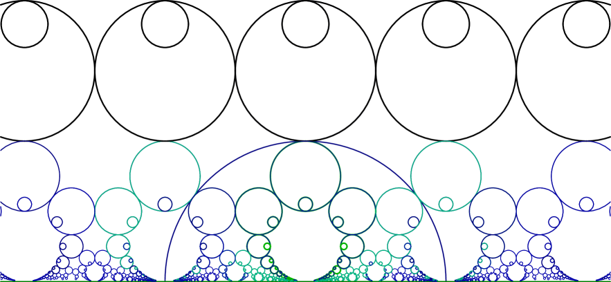
  Figure 2. Action of the modular group on the upper half-plane.

  

  Figure 3. An example of Apollonius problem in three dimensions.

• The package can be used for computer experiments in Möbius–Lie geometry. There is a possibility to create an arrangement of cycles depending on one or several parameters. Then, for particular values of those parameters certain conditions, e.g. concurrency of cycles, may be numerically tested or graphically visualised. It is possible to create animations with gradual change of the parameters, which are especially convenient for illustrations, see Fig. 5 and [Kisil16a].

• Since the library is based on the GiNaC system, which provides a symbolic computation engine, there is a possibility to make fully automatic proofs of various statements in Möbius–Lie geometry. Usage of computer-supported proofs in geometry is already an established practice [Kisil12a, Pech07a] and it is naturally to expect its further rapid growth.

• Last but not least, the combination of classical beauty of Lie sphere geometry and modern computer technologies is a useful pedagogical tool to widen interest in mathematics through visual and hands-on experience.

Computer experiments are especially valuable for Lie geometry of indefinite or nilpotent metrics since our intuition is not elaborated there in contrast to the Euclidean space [Kisil07a, Kisil06a, Kisil05a]. Some advances in the two-dimensional space were achieved recently [Mustafa17a, Kisil12a], however further developments in higher dimensions are still awaiting their researchers.

As a non-trivial example of automated proof accomplished by the figure library for the first time, we present a FLT-invariant version of the classical nine-point theorem [Pedoe95a]*§ I.1 [CoxeterGreitzer]*§ 1.8, cf. Fig. 4(a):

Theorem 7 (Nine-point cycle).

Let $ABC$ be an arbitrary triangle with the orthocenter (the points of intersection of three altitudes) $H$, then the following nine points belongs to the same cycle, which may be a circle or a hyperbola:

1. Foots of three altitudes, that is points of pair-wise intersections $AB$ and $CH$, $AC$ and $BH$, $BC$ and $AH$.

2. Midpoints of sides $AB$, $BC$ and $CA$.

3. Midpoints of intervals $AH$, $BH$ and $CH$.

There are many further interesting properties, e.g. nine-point circle is externally tangent to that triangle three excircles and internally tangent to its incircle as it seen from Fig. 4(a).

To adopt the statement for cycles geometry we need to find a FLT-invariant meaning of the midpoint $A_{m}$ of an interval $BC$, because the equality of distances $BA_{m}$ and $A_{m}C$ is not FLT-invariant. The definition in cycles geometry can be done by either of the following equivalent relations:

• The midpoint $A_{m}$ of an interval $BC$ is defined by the cross-ratio $\frac{BA_{m}}{CA_{m}}:\frac{BI}{CI}=1$, where $I$ is the point at infinity.

• We construct the midpoint $A_{m}$ of an interval $BC$ as the intersection of the interval and the line orthogonal to $BC$ and to the cycle, which uses $BC$ as its diameter. The latter condition means that the cycle passes both points $B$ and $C$ and is orthogonal to the line $BC$.

Both procedures are meaningful if we replace the point at infinity $I$ by an arbitrary fixed point $N$ of the plane. In the second case all lines will be replaced by cycles passing through $N$, for example the line through $B$ and $C$ shall be replaced by a cycle through $B$, $C$ and $N$. If we similarly replace “lines” by “cycles passing through $N$” in Thm. 7 it turns into a valid FLT-invariant version, cf. Fig. 4(b). Some additional properties, e.g. the tangency of the nine-points circle to the ex-/in-circles, are preserved in the new version as well. Furthermore, we can illustrate the connection between two versions of the theorem by an animation, where the infinity is transformed to a finite point $N$ by a continuous one-parameter group of FLT, see. Fig. 5 and further examples at [Kisil16a].

It is natural to test the nine-point theorem in the hyperbolic and the parabolic spaces. Fortunately, it is very easy under the given implementation: we only need to change the defining metric of the point space, this can be done for an already defined figure, see LABEL:sec:example:-nine-points. The corresponding figures Fig. 4(c) and (d) suggest that the hyperbolic version of the theorem is still true in the plain and even FLT-invariant forms. We shall clarify that the hyperbolic version of the Thm. 7 specialises the nine-point conic of a complete quadrilateral [CerinGianella06a, DeVilliers06a]: in addition to the existence of this conic, our theorem specifies its type for this particular arrangement as equilateral hyperbola with the vertical axis of symmetry.

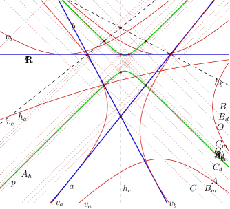
(a) (b)
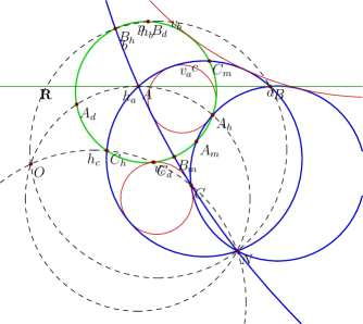
(c) (d)

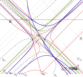
Figure 4. The illustration of the conformal nine-points theorem. The left column is the statement for a triangle with straight sides (the point N is at infinity), the right column is its conformal version (the point N is at the finite part). The first row show the elliptic point space, the second row—the hyperbolic point space. Thus, the top-left picture shows the traditional theorem, three other pictures—its different modifications.

[controls=true,width=.9]50_nine-points-anim

Figure 5. Animated transition between the classical and conformal versions of the nine-point theorem. Use control buttons to activate it. You may need Adobe Acrobat Reader for this feature.

The computational power of the package is sufficient not only to hint that the new theorem is true but also to make a complete proof. To this end we define an ensemble of cycles with exactly same interrelations, but populate the generation-0 with points $A$, $B$ and $C$ with symbolic coordinates, that is, objects of the GiNaC class realsymbol. Thus, the entire figure defined from them will be completely general. Then, we may define the hyperbola passing through three bases of altitudes and check by the symbolic computations that this hyperbola passes another six “midpoints” as well, see LABEL:sec:prov-theor-symb .

In the parabolic space the nine-point Thm. 7 is not preserved in this manner. It is already observed [Kisil12a, Kisil05a, Kisil15a, Kisil07a, Kisil09e, Kisil11a, Mustafa17a, BarrettBolt10a], that the degeneracy of parabolic metric in the point space requires certain revision of traditional definitions. The parabolic variation of nine-point theorem may prompt some further considerations as well. An expanded discussion of various aspects of the nine-point construction shall be the subject of a separate paper.

5. To Do List

The library is still under active development. Along with continuous bug fixing there is an intention to extend both functionality and usability. Here are several nearest tasks planned so far:

• Expand class subfigure in way suitable for encoding loxodromes and other objects of an extended Möbius–Lie geometry [KisilReid18a, Kisil15a].

• Add non-point transformations, extending the package to Lie sphere geometry.

• Add a method which will apply a FLT to the entire figure.

• Provide an effective parametrisation of solutions of a single quadratics condition.

• Expand drawing facilities in three dimensions to hyperboloids and paraboloids.

• Create Graphical User Interface which will open the library to users without programming skills.

• Investigate cloud computing options which can free a user from the burden of installation.

Being an open-source project the library is open for contributions and suggestions of other developers and users.

Appendix A Examples of Usage

This section presents several examples, which may be used for quick start. We begin with very elementary one, but almost all aspects of the library usage will be illustrated by the end of this section. See the beginning of Section LABEL:sec:publ-meth-figure for installation advise. The collection of these programmes is also serving as a test suit for the library.

LABEL:NWppJ6t-1fWRR8-1$\langle$separating chunk LABEL:NWppJ6t-1fWRR8-1$\rangle$$\equiv$        $\mathord{\mbox{\hyperlink{noweb.NWppJ6t-1fWRR8-2}{\ref{NWppJ6t-1fWRR8-2}}}}\,\mathord{\triangleright}$                                                                                                     

A.1. Hello, Cycle!

This is a minimalist example showing how to obtain a simple drawing of
cycles in non-Euclidean geometry. Of course, we are starting from the
library header file.

LABEL:NWppJ6t-3rkk58-1$\langle$hello-cycle.cpp LABEL:NWppJ6t-3rkk58-1$\rangle$$\equiv$        $\mathord{\mbox{\hyperlink{noweb.NWppJ6t-3rkk58-2}{\ref{NWppJ6t-3rkk58-2}}}}\,\mathord{\triangleright}$                                                                                                     
$\langle$license LABEL:NWppJ6t-ZXuKx-1$\rangle$
#include "figure.h"
$\langle$using all namespaces LABEL:NWppJ6t-3uHj2c-1$\rangle$
int main(){

Defines:

main, never used.

Uses figure.

To save keystrokes, we use the following namespaces.

LABEL:NWppJ6t-3uHj2c-1$\langle$using all namespaces LABEL:NWppJ6t-3uHj2c-1$\rangle$$\equiv$        (noweb.?? noweb.?? noweb.?? noweb.?? noweb.?? noweb.?? noweb.?? noweb.?? 0—1)                                                                                                     
using namespace std;
using namespace GiNaC;
using namespace MoebInv;

Defines:

MoebInv, never used.

We declare the figure F which will be constructed with the
default elliptic metric in two dimensions.

LABEL:NWppJ6t-3rkk58-2$\langle$hello-cycle.cpp LABEL:NWppJ6t-3rkk58-1$\rangle$$\mathord{+}\mathord{\equiv}$        $\mathord{\triangleleft}\,\mathord{\mbox{\hyperlink{noweb.NWppJ6t-3rkk58-1}{\ref{NWppJ6t-3rkk58-1}}}}$  $\mathord{\mbox{\hyperlink{noweb.NWppJ6t-3rkk58-3}{\ref{NWppJ6t-3rkk58-3}}}}\,\mathord{\triangleright}$                                                                                                     
figure F;

Defines:

figure, never used.

Next we define a couple of points A and B. Every point is
added to F by giving its explicit coordinates as a lst and a
string, which will be used to label the point. The returned value is a
GiNaC expression of symbol class, which will be used as a key
of the respective point. All points are added to the zero generation.

LABEL:NWppJ6t-3rkk58-3$\langle$hello-cycle.cpp LABEL:NWppJ6t-3rkk58-1$\rangle$$\mathord{+}\mathord{\equiv}$        $\mathord{\triangleleft}\,\mathord{\mbox{\hyperlink{noweb.NWppJ6t-3rkk58-2}{\ref{NWppJ6t-3rkk58-2}}}}$  $\mathord{\mbox{\hyperlink{noweb.NWppJ6t-3rkk58-4}{\ref{NWppJ6t-3rkk58-4}}}}\,\mathord{\triangleright}$                                                                                                     
ex A=F.add_point(lst{-1,.5},"A");
ex B=F.add_point(lst{1,1.5},"B");

Defines:

add_point, never used.

Uses ex.

Now we add a “line” in the Lobachevsky half-plane. It passes both
points A and B and is orthogonal to the real line. The real
line and the point at infinity were automatically added to F at
its initialisation. The real line is accessible as
F.get_real_line() method in figure class. A cycle
passes a point if it is orthogonal to the cycle defined by this
point. Thus, the line is defined through a list of three
orthogonalities~[Kisil06a] [Kisil12a]*Defn.~6.1
(other pre-defined relations between cycles are listed in
Section~LABEL:sec:publ-meth-cycl). We also supply a string to label
this cycle. The returned valued is a symbol, which is a key for this
cycle.

LABEL:NWppJ6t-3rkk58-4$\langle$hello-cycle.cpp LABEL:NWppJ6t-3rkk58-1$\rangle$$\mathord{+}\mathord{\equiv}$        $\mathord{\triangleleft}\,\mathord{\mbox{\hyperlink{noweb.NWppJ6t-3rkk58-3}{\ref{NWppJ6t-3rkk58-3}}}}$  $\mathord{\mbox{\hyperlink{noweb.NWppJ6t-3rkk58-5}{\ref{NWppJ6t-3rkk58-5}}}}\,\mathord{\triangleright}$                                                                                                     
ex a=F.add_cycle_rel(lst{is_orthogonal(A),is_orthogonal(B),is_orthogonal(F.get_real_line())},"a");

Defines:

add_cycle_rel, never used.

get_real_line, never used.

Uses ex and is_orthogonal.

Now, we draw our figure to a file. Its format (e.g. EPS, PDF, PNG,
etc.) is determined by your default Asymptote settings. This can be
overwritten if a format is explicitly requested, see examples below.
The output is shown at Figure~6.

LABEL:NWppJ6t-3rkk58-5$\langle$hello-cycle.cpp LABEL:NWppJ6t-3rkk58-1$\rangle$$\mathord{+}\mathord{\equiv}$        $\mathord{\triangleleft}\,\mathord{\mbox{\hyperlink{noweb.NWppJ6t-3rkk58-4}{\ref{NWppJ6t-3rkk58-4}}}}$                                                                                                     
F.asy_write(300,-3,3,-3,3,"lobachevsky-line");
return 0;
}

Defines:

asy_write, never used.

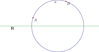
Figure 6. Lobachevky line.

LABEL:NWppJ6t-1fWRR8-2$\langle$separating chunk LABEL:NWppJ6t-1fWRR8-1$\rangle$$\mathord{+}\mathord{\equiv}$        $\mathord{\triangleleft}\,\mathord{\mbox{\hyperlink{noweb.NWppJ6t-1fWRR8-1}{\ref{NWppJ6t-1fWRR8-1}}}}$  $\mathord{\mbox{\hyperlink{noweb.NWppJ6t-1fWRR8-3}{\ref{NWppJ6t-1fWRR8-3}}}}\,\mathord{\triangleright}$                                                                                                     

A.2. Animated cycle

We use the similar construction to make an animation.

LABEL:NWppJ6t-1kKRnF-1$\langle$hello-cycle-anim.cpp LABEL:NWppJ6t-1kKRnF-1$\rangle$$\equiv$        $\mathord{\mbox{\hyperlink{noweb.NWppJ6t-1kKRnF-2}{\ref{NWppJ6t-1kKRnF-2}}}}\,\mathord{\triangleright}$                                                                                                     
$\langle$license LABEL:NWppJ6t-ZXuKx-1$\rangle$
#include "figure.h"
$\langle$using all namespaces LABEL:NWppJ6t-3uHj2c-1$\rangle$
int main(){

Defines:

main, never used.

Uses figure.

It is preferable to freeze a figure with a symbolic parameter in
order to avoid useless but expensive symbolic computations. It will be
automatically unfreeze by asy_animate method below.

LABEL:NWppJ6t-1kKRnF-2$\langle$hello-cycle-anim.cpp LABEL:NWppJ6t-1kKRnF-1$\rangle$$\mathord{+}\mathord{\equiv}$        $\mathord{\triangleleft}\,\mathord{\mbox{\hyperlink{noweb.NWppJ6t-1kKRnF-1}{\ref{NWppJ6t-1kKRnF-1}}}}$  $\mathord{\mbox{\hyperlink{noweb.NWppJ6t-1kKRnF-3}{\ref{NWppJ6t-1kKRnF-3}}}}\,\mathord{\triangleright}$                                                                                                     
figure F=figure().freeze();
symbol t("t");

Defines:

freeze, never used.

unfreeze, never used.

Uses figure.

This time the point A on the figure depends from the above parameter
t and the point B is fixed as before.

LABEL:NWppJ6t-1kKRnF-3$\langle$hello-cycle-anim.cpp LABEL:NWppJ6t-1kKRnF-1$\rangle$$\mathord{+}\mathord{\equiv}$        $\mathord{\triangleleft}\,\mathord{\mbox{\hyperlink{noweb.NWppJ6t-1kKRnF-2}{\ref{NWppJ6t-1kKRnF-2}}}}$  $\mathord{\mbox{\hyperlink{noweb.NWppJ6t-1kKRnF-4}{\ref{NWppJ6t-1kKRnF-4}}}}\,\mathord{\triangleright}$                                                                                                     
ex A=F.add_point(lst{-1$\ast$t,.5$\ast$t+.5},"A");
ex B=F.add_point(lst{1,1.5},"B");

Uses add_point and ex.

The Lobachevsky line a is defined exactly as in the previous
example but is implicitly (through A) depending on t now.

LABEL:NWppJ6t-1kKRnF-4$\langle$hello-cycle-anim.cpp LABEL:NWppJ6t-1kKRnF-1$\rangle$$\mathord{+}\mathord{\equiv}$        $\mathord{\triangleleft}\,\mathord{\mbox{\hyperlink{noweb.NWppJ6t-1kKRnF-3}{\ref{NWppJ6t-1kKRnF-3}}}}$  $\mathord{\mbox{\hyperlink{noweb.NWppJ6t-1kKRnF-5}{\ref{NWppJ6t-1kKRnF-5}}}}\,\mathord{\triangleright}$                                                                                                     
ex a=F.add_cycle_rel(lst{is_orthogonal(A),is_orthogonal(B),is_orthogonal(F.get_real_line())},"a");

Uses add_cycle_rel, ex, get_real_line, and is_orthogonal.

The new straight line b is defined as a cycle passing
(orthogonal to) the point at infinity. It is accessible by
get_infinity method.

LABEL:NWppJ6t-1kKRnF-5$\langle$hello-cycle-anim.cpp LABEL:NWppJ6t-1kKRnF-1$\rangle$$\mathord{+}\mathord{\equiv}$        $\mathord{\triangleleft}\,\mathord{\mbox{\hyperlink{noweb.NWppJ6t-1kKRnF-4}{\ref{NWppJ6t-1kKRnF-4}}}}$  $\mathord{\mbox{\hyperlink{noweb.NWppJ6t-1kKRnF-6}{\ref{NWppJ6t-1kKRnF-6}}}}\,\mathord{\triangleright}$                                                                                                     
ex b=F.add_cycle_rel(lst{is_orthogonal(A),is_orthogonal(B),is_orthogonal(F.get_infinity())},"b");

Defines:

get_infinity, never used.

Uses add_cycle_rel, ex, and is_orthogonal.

Now we define the set of values for the parameter t which will
be used for substitution into the figure.

LABEL:NWppJ6t-1kKRnF-6$\langle$hello-cycle-anim.cpp LABEL:NWppJ6t-1kKRnF-1$\rangle$$\mathord{+}\mathord{\equiv}$        $\mathord{\triangleleft}\,\mathord{\mbox{\hyperlink{noweb.NWppJ6t-1kKRnF-5}{\ref{NWppJ6t-1kKRnF-5}}}}$  $\mathord{\mbox{\hyperlink{noweb.NWppJ6t-1kKRnF-7}{\ref{NWppJ6t-1kKRnF-7}}}}\,\mathord{\triangleright}$                                                                                                     
lst val;
for (int i=0; i$<$40; $\scriptscriptstyle+\kern-1.0pt+$i)
val.append(t$\equiv$numeric(i+2,30));

Uses numeric.

Finally animations in different formats are created similarly to the
static picture from the previous example.

LABEL:NWppJ6t-1kKRnF-7$\langle$hello-cycle-anim.cpp LABEL:NWppJ6t-1kKRnF-1$\rangle$$\mathord{+}\mathord{\equiv}$        $\mathord{\triangleleft}\,\mathord{\mbox{\hyperlink{noweb.NWppJ6t-1kKRnF-6}{\ref{NWppJ6t-1kKRnF-6}}}}$                                                                                                     
F.asy_animate(val,500,-2.2,3,-2,2,"lobachevsky-anim","mng");
F.asy_animate(val,300,-2.2,3,-2,2,"lobachevsky-anim","pdf");
return 0;
}

Defines:

asy_animate, never used.

The second command creates two files: lobachevsky-anim.pdf
and _lobachevsky-anim.pdf (notice the underscore (_) in
front of the file name, which makes the difference). The former is a
stand-alone PDF file containing the desired animation. The latter may
be embedded into another PDF document as shown on
Fig.~7. To this end the LaTeX file need to
have the command

\usepackage{animate}

in its preamble. To include the animation we use the command:

\animategraphics[controls]{50}{_lobachevsky-anim}{}{}

More options can be found in the
documentation
of animate package.
Finally, the LaTeX file need to be compiled with the
pdfLaTeX command.

[controls]50˙lobachevsky-anim

Figure 7. Animated Lobachevsky line: use
the control buttons to run the animation. You may need
Adobe Acrobat Reader for this feature.

LABEL:NWppJ6t-1fWRR8-3$\langle$separating chunk LABEL:NWppJ6t-1fWRR8-1$\rangle$$\mathord{+}\mathord{\equiv}$        $\mathord{\triangleleft}\,\mathord{\mbox{\hyperlink{noweb.NWppJ6t-1fWRR8-2}{\ref{NWppJ6t-1fWRR8-2}}}}$  $\mathord{\mbox{\hyperlink{noweb.NWppJ6t-1fWRR8-4}{\ref{NWppJ6t-1fWRR8-4}}}}\,\mathord{\triangleright}$                                                                                                     

A.3. An illustration of the modular group action

The library allows to build figures out of cycles which are obtained
from each other by means of FLT. We are going to
illustrate this by the action of the modular group
$\mathrm{SL}_2(\mathbb{Z})$ on a single
circle~[StewartTall02a]*§~14.4. We repeatedly apply FLT $T=\@break\begin{pmatrix}\@break 1&1\\ 0&1\@break\end{pmatrix}$
for translations and $S=\@break\begin{pmatrix}\@break 0&-1\\ 1&0\@break\end{pmatrix}$ for the inversion in the unit circle.

Here is the standard start of a programme with some additional
variables being initialised.

LABEL:NWppJ6t-2SYluR-1$\langle$modular-group.cpp LABEL:NWppJ6t-2SYluR-1$\rangle$$\equiv$        $\mathord{\mbox{\hyperlink{noweb.NWppJ6t-2SYluR-2}{\ref{NWppJ6t-2SYluR-2}}}}\,\mathord{\triangleright}$                                                                                                     
$\langle$license LABEL:NWppJ6t-ZXuKx-1$\rangle$
#include "figure.h"
$\langle$using all namespaces LABEL:NWppJ6t-3uHj2c-1$\rangle$
int main(){
char buffer [50];
int steps=3, trans=15;
double epsilon=0.00001; // square of radius for a circle to be ignored
figure F;

Defines:

main, never used.

Uses epsilon and figure.

We will use the metric associated to the figure, it can be extracted
by get_point_metric method.

LABEL:NWppJ6t-2SYluR-2$\langle$modular-group.cpp LABEL:NWppJ6t-2SYluR-1$\rangle$$\mathord{+}\mathord{\equiv}$        $\mathord{\triangleleft}\,\mathord{\mbox{\hyperlink{noweb.NWppJ6t-2SYluR-1}{\ref{NWppJ6t-2SYluR-1}}}}$  $\mathord{\mbox{\hyperlink{noweb.NWppJ6t-2SYluR-3}{\ref{NWppJ6t-2SYluR-3}}}}\,\mathord{\triangleright}$                                                                                                     
ex e=F.get_point_metric();

Defines:

get_point_metric, never used.

Uses ex.

Firstly, we add to the figure an initial cycle and, then, add new
generations of its shifts and reflections.

LABEL:NWppJ6t-2SYluR-3$\langle$modular-group.cpp LABEL:NWppJ6t-2SYluR-1$\rangle$$\mathord{+}\mathord{\equiv}$        $\mathord{\triangleleft}\,\mathord{\mbox{\hyperlink{noweb.NWppJ6t-2SYluR-2}{\ref{NWppJ6t-2SYluR-2}}}}$  $\mathord{\mbox{\hyperlink{noweb.NWppJ6t-2SYluR-4}{\ref{NWppJ6t-2SYluR-4}}}}\,\mathord{\triangleright}$                                                                                                     
ex a=F.add_cycle(cycle2D(lst{0,numeric(3,2)},e,numeric(1,4)),"a");
ex c=F.add_cycle(cycle2D(lst{0,numeric(11,6)},e,numeric(1,36)),"c");
for (int i=0; i$<$steps;$\scriptscriptstyle+\kern-1.0pt+$i) {

Uses add_cycle, ex, and numeric.

We want to shift all cycles in the previous
generation. Their key are grasped by get_all_keys method.

LABEL:NWppJ6t-2SYluR-4$\langle$modular-group.cpp LABEL:NWppJ6t-2SYluR-1$\rangle$$\mathord{+}\mathord{\equiv}$        $\mathord{\triangleleft}\,\mathord{\mbox{\hyperlink{noweb.NWppJ6t-2SYluR-3}{\ref{NWppJ6t-2SYluR-3}}}}$  $\mathord{\mbox{\hyperlink{noweb.NWppJ6t-2SYluR-5}{\ref{NWppJ6t-2SYluR-5}}}}\,\mathord{\triangleright}$                                                                                                     
lst L=ex_to$<$lst$>$(F.get_all_keys(2$\ast$i,2$\ast$i));
if (L.nops() $\equiv$ 0) {
cout $\ll$ "Terminate on iteration " $\ll$ i $\ll$ endl;
break;
}

Defines:

get_all_keys, never used.

Uses nops.

Each cycle with the collected key is shifted horizontally by an
integer $t$ in range [$-$trans,trans]. This done by
moebius_transform relations and it is our responsibility to
produce proper Clifford-valued entries to the matrix,
see~[Kisil05a]*§~2.1 for an advise.

LABEL:NWppJ6t-2SYluR-5$\langle$modular-group.cpp LABEL:NWppJ6t-2SYluR-1$\rangle$$\mathord{+}\mathord{\equiv}$        $\mathord{\triangleleft}\,\mathord{\mbox{\hyperlink{noweb.NWppJ6t-2SYluR-4}{\ref{NWppJ6t-2SYluR-4}}}}$  $\mathord{\mbox{\hyperlink{noweb.NWppJ6t-2SYluR-6}{\ref{NWppJ6t-2SYluR-6}}}}\,\mathord{\triangleright}$                                                                                                     
for (const auto& k: L) {
lst L1=ex_to$<$lst$>$(F.get_cycle(k));
for (auto x: L1) {
for (int t=-trans; t$\leq$trans;$\scriptscriptstyle+\kern-1.0pt+$t) {
sprintf (buffer, "%s-%dt%d",ex_to$<$symbol$>$(k).get_name().c_str(),i,t);

Uses get_cycle and k.

We shift initial cycles by zero in order to have their copies in the this generation.

LABEL:NWppJ6t-2SYluR-6$\langle$modular-group.cpp LABEL:NWppJ6t-2SYluR-1$\rangle$$\mathord{+}\mathord{\equiv}$        $\mathord{\triangleleft}\,\mathord{\mbox{\hyperlink{noweb.NWppJ6t-2SYluR-5}{\ref{NWppJ6t-2SYluR-5}}}}$  $\mathord{\mbox{\hyperlink{noweb.NWppJ6t-2SYluR-7}{\ref{NWppJ6t-2SYluR-7}}}}\,\mathord{\triangleright}$                                                                                                     
if ((t $\neq$0 $\vee$ i $\equiv$0)

To simplify the picture we are skipping circles whose radii would be
smaller than the threshold.

LABEL:NWppJ6t-2SYluR-7$\langle$modular-group.cpp LABEL:NWppJ6t-2SYluR-1$\rangle$$\mathord{+}\mathord{\equiv}$        $\mathord{\triangleleft}\,\mathord{\mbox{\hyperlink{noweb.NWppJ6t-2SYluR-6}{\ref{NWppJ6t-2SYluR-6}}}}$  $\mathord{\mbox{\hyperlink{noweb.NWppJ6t-2SYluR-8}{\ref{NWppJ6t-2SYluR-8}}}}\,\mathord{\triangleright}$                                                                                                     
$\wedge$ $\neg$ ((ex_to$<$cycle$>$(x).det()-(pow(t,2)-1)$\ast$epsilon).evalf()$<$0)){
ex b=F.add_cycle_rel(moebius_transform(k,true,
lst{dirac_ONE(),t$\ast$e.subs(e.op(1).op(0)$\equiv$0),0,dirac_ONE()}),buffer);

Defines:

moebius_transform, never used.

Uses add_cycle_rel, epsilon, evalf, ex, k, op, and subs.

We want the colour of a cycle reflect its generation, smaller cycles
also need to be drawn by a finer pen. This can be set for each cycle
by set_asy_style method.

LABEL:NWppJ6t-2SYluR-8$\langle$modular-group.cpp LABEL:NWppJ6t-2SYluR-1$\rangle$$\mathord{+}\mathord{\equiv}$        $\mathord{\triangleleft}\,\mathord{\mbox{\hyperlink{noweb.NWppJ6t-2SYluR-7}{\ref{NWppJ6t-2SYluR-7}}}}$  $\mathord{\mbox{\hyperlink{noweb.NWppJ6t-2SYluR-9}{\ref{NWppJ6t-2SYluR-9}}}}\,\mathord{\triangleright}$                                                                                                     
sprintf (buffer, "rgb(0,0,%.2f)+%.3f" ,1-1$\div$(i+1.),1$\div$(i+1.5));
F.set_asy_style(b,buffer);
}
}
}
}

Defines:

rgb, never used.

set_asy_style, never used.

Similarly, we collect all key from the previous generation cycles
to make their reflection in the unit circle.

LABEL:NWppJ6t-2SYluR-9$\langle$modular-group.cpp LABEL:NWppJ6t-2SYluR-1$\rangle$$\mathord{+}\mathord{\equiv}$        $\mathord{\triangleleft}\,\mathord{\mbox{\hyperlink{noweb.NWppJ6t-2SYluR-8}{\ref{NWppJ6t-2SYluR-8}}}}$  $\mathord{\mbox{\hyperlink{noweb.NWppJ6t-2SYluR-A}{\ref{NWppJ6t-2SYluR-A}}}}\,\mathord{\triangleright}$                                                                                                     
if (i$<$steps-1)
L=ex_to$<$lst$>$(F.get_all_keys(2$\ast$i+1,2$\ast$i+1));
else
L=lst{};
for (const auto& k: L) {
sprintf (buffer, "%ss",ex_to$<$symbol$>$(k).get_name().c_str());

Uses get_all_keys and k.

This tame we keep things simple and are using sl2_transform
relation, all Clifford algebra adjustments are taken by the
library. The drawing style is setup accordingly.

LABEL:NWppJ6t-2SYluR-A$\langle$modular-group.cpp LABEL:NWppJ6t-2SYluR-1$\rangle$$\mathord{+}\mathord{\equiv}$        $\mathord{\triangleleft}\,\mathord{\mbox{\hyperlink{noweb.NWppJ6t-2SYluR-9}{\ref{NWppJ6t-2SYluR-9}}}}$  $\mathord{\mbox{\hyperlink{noweb.NWppJ6t-2SYluR-B}{\ref{NWppJ6t-2SYluR-B}}}}\,\mathord{\triangleright}$                                                                                                     
ex b=F.add_cycle_rel(sl2_transform(k,true,lst{0,-1,1,0}),buffer);
sprintf (buffer, "rgb(0,0.7,%.2f)+%.3f" ,1-1$\div$(i+1.),1$\div$(i+1.5));
F.set_asy_style(b,buffer);
}
}

Defines:

sl2_transform, never used.

Uses add_cycle_rel, ex, k, rgb, and set_asy_style.

Finally, we draw the picture. This time we do not want cycles label
to appear, thus the last parameter with_labels of asy_write is
false. We also want to reduce the size of Asymptote file and
will not print headers of cycles, thus specifying
with_header=true. The remaining parameters are explicitly assigned
their default values.

LABEL:NWppJ6t-2SYluR-B$\langle$modular-group.cpp LABEL:NWppJ6t-2SYluR-1$\rangle$$\mathord{+}\mathord{\equiv}$        $\mathord{\triangleleft}\,\mathord{\mbox{\hyperlink{noweb.NWppJ6t-2SYluR-A}{\ref{NWppJ6t-2SYluR-A}}}}$                                                                                                     
ex u=F.add_cycle(cycle2D(lst{0,0},e,numeric(1)),"u");
F.asy_write(300,-2.17,2.17,0,2,"modular-group","pdf",default_asy,default_label,true,false,0,"rgb(0,.9,0)+4pt",true,false);
return 0;
}

Defines:

asy_write, never used.

Uses add_cycle, ex, numeric, and rgb.

LABEL:NWppJ6t-1fWRR8-4$\langle$separating chunk LABEL:NWppJ6t-1fWRR8-1$\rangle$$\mathord{+}\mathord{\equiv}$        $\mathord{\triangleleft}\,\mathord{\mbox{\hyperlink{noweb.NWppJ6t-1fWRR8-3}{\ref{NWppJ6t-1fWRR8-3}}}}$  $\mathord{\mbox{\hyperlink{noweb.NWppJ6t-1fWRR8-5}{\ref{NWppJ6t-1fWRR8-5}}}}\,\mathord{\triangleright}$