HST Emission Line Galaxies at $z\sim 2$: Comparing Physical Properties of Lyman Alpha and Optical Emission Line Selected Galaxies

Abstract

We compare the physical and morphological properties of $z\sim 2$ Ly$\alpha$ emitting galaxies (LAEs) identified in the HETDEX Pilot Survey and narrow band studies with those of $z\sim 2$ optical emission line galaxies (oELGs) identified via HST WFC3 infrared grism spectroscopy. Both sets of galaxies extend over the same range in stellar mass ($7.5<\log M/M_{\odot}<10.5$), size ($0.5<R<3.0$ kpc), and star-formation rate ($\sim 1<{\rm SFR}<100\,M_{\odot}$ yr^-1). Remarkably, a comparison of the most commonly used physical and morphological parameters — stellar mass, half-light radius, UV slope, star formation rate, ellipticity, nearest neighbor distance, star formation surface density, specific star formation rate, [O III] luminosity, and [O III] equivalent width — reveals no statistically significant differences between the populations. This suggests that the processes and conditions which regulate the escape of Ly$\alpha$ from a $z\sim 2$ star-forming galaxy do not depend on these quantities. In particular, the lack of dependence on the UV slope suggests that Ly$\alpha$ emission is not being significantly modulated by diffuse dust in the interstellar medium. We develop a simple model of Ly$\alpha$ emission that connects LAEs to all high-redshift star forming galaxies where the escape of Ly$\alpha$ depends on the sightline through the galaxy. Using this model, we find that mean solid angle for Ly$\alpha$ escape is $\Omega_{{\rm Ly}\alpha}=2.4\pm 0.8$ steradians; this value is consistent with those calculated from other studies.

1 Introduction

Ly$\alpha$ emitting galaxies (LAEs) are one of the most important constituents of the high-redshift universe. Although rare at $z\lesssim 0.3$ (Deharveng et al., 2008; Cowie et al., 2010), LAEs become more common (and more luminous) with increasing redshift, and by $z\sim 6$, they comprise the bulk of the observed star-forming galaxy population (Cassata et al., 2015; Ouchi et al., 2010; Ciardullo et al., 2012; Bouwens et al., 2010). The clustering properties of $z\sim 3$ LAEs suggest a connection with today’s $L^{*}$ galaxies (Gawiser et al., 2007; Guaita et al., 2010), while LAEs at larger redshifts typically have higher biases (Ouchi et al., 2010).

Ly$\alpha$ emitters are generally considered to be low-mass, dust-poor systems, as the resonant nature of the Ly$\alpha$ line makes its escape from large, dusty systems problematic (e.g. Verhamme et al., 2006; Gawiser et al., 2006; Gronwall et al., 2007; Finkelstein et al., 2008, 2009; Schaerer et al., 2011). However, the association of LAEs with low-mass galaxies is an oversimplification: multiple studies have demonstrated that luminous Ly$\alpha$ emitters have a very wide range of stellar mass (at least three dex or more), and that not all LAEs are dust-poor (Finkelstein et al., 2009; Nilsson et al., 2011; Hagen et al., 2014; Vargas et al., 2014). This result calls into question the relationship between LAEs and other denizens of the high-redshift galaxy zoo. Hydrodynamic models that include Ly$\alpha$ radiative transfer predict that galaxy morphology and inclination should play an important role in determining the observability of Ly$\alpha$ (e.g., Verhamme et al., 2012; Yajima et al., 2012; Behrens et al., 2014), and studies have shown that the presence of Ly$\alpha$ is correlated with galaxy size and ellipticity (e.g., Shibuya et al., 2014a). It is also possible that Ly$\alpha$ emission is facilitated by a low column density of neutral hydrogen (Shibuya et al., 2014b; Song et al., 2014), but merger activity appears unrelated to the phenomenon (Shibuya et al., 2014a).

One difficulty with understanding the systematics of Ly$\alpha$ is that to date, almost all the comparison samples of non-Ly$\alpha$ emitting star-forming galaxies have been continuum-selected high-mass systems, such as Lyman-break galaxies (LBGs), with sizes and star formation rates (SFRs) that are quite different from that of the typical LAE (e.g., Malhotra et al., 2012). Only very recently, have LAEs been analyzed alongside of galaxies with a similar stellar mass range (Song et al., 2014; Hathi et al., 2015). We address this problem by comparing the physical properties of photometrically- and spectroscopically-selected $z\sim 2$ LAEs (Guaita et al., 2010; Adams et al., 2011) to those of optical emission line galaxies (oELGs) at the same redshift (Zeimann et al., 2014). Because our oELGs have similar masses, sizes, and star-formation rates as their LAE counterparts, we can analyze the two populations differentially, and identify those properties most important for the escape of Ly$\alpha$ photons.

In Section 2 we discuss our sample selection, in Section 3 we describe our analysis, and we present our findings in Section 4. We adopt the standard concordance cosmology of $h=0.7$, $\Omega_{m}=0.3$, $\Omega_{\Lambda}=0.7$, and $\Omega_{k}=0$ (Ade et al., 2014).

2 Sample Selection

Most previous studies of the physical properties of Ly$\alpha$ emitters have used continuum-selected galaxies as the experiment’s control sample (e.g., Malhotra et al., 2012). Such an assignment is clearly not ideal: systems such as Lyman-break and $BzK$ galaxies are not only more massive than typical LAEs, but their clustering properties indicate a very different evolutionary path. What is needed is a set of galaxies with roughly the same stellar mass, star-formation rate, and size as the LAEs under investigation. As our analysis will show, the physical properties of our sample of oELGs are indeed well-matched to those of our program LAEs.

Our comparison set of $z\sim 2$ oELGs was identified using the Hubble Space Telescope’s WFC3 camera and its $R=130$ G141 grism. A full description of these data, procured by the 3D-HST and AGHAST surveys (GO-11600, 12177, and 12328; Brammer et al., 2012; Weiner et al., 2014), is given in Zeimann et al. (2014). In brief, a total of $\sim 350$ arcmin² of the COSMOS (Scoville et al., 2007), GOODS-N, and GOODS-S (Giavalisco et al., 2004) fields were surveyed over the wavelength range $1.08~{}\mu{\rm m}<\lambda<1.68~{}\mu$m down to a 50% monochromatic completeness flux limit of $F\sim 10^{-17}$ ergs cm^-2 s^-1. For each object brighter than F140W = 26, a spectrum was extracted, flux-calibrated, checked for contamination, continuum-subtracted, and visually inspected for evidence of emission lines. Galaxies with unambiguous redshifts between $1.90<z<2.35$ were then selected via the identification of at least two of the emission lines of [O II] $\lambda 3727$, [Ne III] $\lambda 3869$, H$\delta$, H$\gamma$, H$\beta$, and [O III] $\lambda\lambda 4959,5007$. Although $\sim 15\%$ of the region’s galaxies were unmeasurable due to contamination from overlapping spectra, this procedure still produced a sample of 245 star-forming galaxies in the targeted redshift range with the distinctively-shaped [O III] blend typically being the brightest feature.

The LAEs for our analysis are drawn from two sources. The first was the Hobby Eberly Telescope Dark Energy Experiment (HETDEX) Pilot Survey (HPS; Adams et al., 2011; Blanc et al., 2011), a blind integral field spectroscopic study that included 107 arcmin² of the COSMOS and GOODS-N fields. At $z\sim 2.2$, 50% of the HPS pointings reached a $5\,\sigma$ monochromatic flux limit of $1.3\times 10^{-16}$ ergs cm^-2 s^-1 (or $\log L({\rm Ly}\alpha)=42.68$ ergs) and 90% reached $2.5\times 10^{-16}$ ergs cm^-2 s^-1 ($\log L({\rm Ly}\alpha)=42.96$ ergs). Simulations demonstrate that above these flux limits, the recovery fraction of emission lines was better than 95% for equivalent widths greater than 5 Å, and higher than 90% for equivalent widths as small as 1 Å (Adams et al., 2011). The HPS identified 67 LAEs in the COSMOS and GOODS-N fields, but for consistency with our comparison sample, we consider only those 11 LAEs between $1.90<z<2.35$. Over this redshift range, the luminosity limits of the HPS survey are roughly constant with redshift (Blanc et al., 2011).

Our second source of LAEs is a narrow-band survey for $z\sim 2$ Ly$\alpha$ sources in the Extended Chandra Deep Field South (ECDF-S). By using a 50 Å interference filter and the CTIO 4-m Mosaic camera, Guaita et al. (2010) identified LAEs with Ly$\alpha$ fluxes brighter than $2\times 10^{-17}$ ergs cm^-2 s^-1 and redshifts $2.04\lesssim z\lesssim 2.08$. (See Ciardullo et al. (2012) for more details on this dataset.) A total of 17 of the LAEs brighter than the 90% completeness limit of Ciardullo et al. (2012) fall in the 3D-HST’s GOODS-S region. Thus, the combination of the HPS and narrowband datasets yields a sample of 28 Ly$\alpha$ emitters.

We note that the volume of space covered by both the LAE and oELG surveys is considerably smaller than that observed by each technique individually. For example, while the total number of $1.90<z<2.35$ galaxies found via the HST IR grism is 245, only 63 oELGs fall in regions covered by the HPS or the ECDF-S narrow-band survey. Of these, just 12, or roughly 20%, are also classified as LAEs (Ciardullo et al., 2014). If we remove these 12 dual-classification objects from the set of oELGs, we are left with a sample of 233 galaxies selected via their optical emission lines, and 28 galaxies detected via Ly$\alpha$. For most of the comparisons that follow, we use the entire sample of 233 oELGs to the 28 LAEs: only when considering the solid angle of Ly$\alpha$ escape do we use the subset of 63 oELGs in the regions of survey overlap.

To study the conditions which facilitate the escape of Ly$\alpha$ emission, one would ideally begin with a large, homogeneously selected sample of galaxies and then consider which objects emit in Ly$\alpha$ and which do not. Unfortunately, while such a procedure works well for the continuum-bright Lyman break objects (Steidel et al., 1996a, b; Kornei et al., 2010; Le Fèvre et al., 2015), it is difficult to implement for objects selected via their emission lines. As will be shown below, many of our oELGs and LAEs are quite faint in the continuum, so comprehensive surveys for both the Ly$\alpha$ and rest-frame optical emission lines would require prohibitively deep exposures. In fact, previous surveys have shown that the global escape fraction of Ly$\alpha$ from the $z\sim 3$ universe is only $\sim 5\%$, and that there is generally little overlap between samples of galaxies selected via their Ly$\alpha$ and Balmer emission lines (Hayes et al., 2010; Ciardullo et al., 2014). Nevertheless, as we shall show, we can still examine the properties which facilitate Ly$\alpha$ escape using our Ly$\alpha$ and optical emission line selected galaxies.

3 Physical Properties

To determine the photometric properties of both our LAEs and the emission-line selected comparison sample, we took advantage of the multi-wavelength catalog of Skelton et al. (2014), which extends over the CANDELS fields of GOODS-S, GOODS-N, and COSMOS (Grogin et al., 2011). This database begins with the deep, co-added F125W + F140W + F160W images from HST and then adds in the results of 30 distinct ground- and space-based imaging programs to produce a homogeneous, PSF-matched set of broad- and intermediate-band flux densities covering the entire wavelength range from $0.35~{}\mu$m to $8.0~{}\mu$m. In the COSMOS field, this dataset contains photometry in 44 separate bandpasses, with measurements from HST, Spitzer, Subaru, and a host of smaller ground-based telescopes. In GOODS-N, the data come from five different observatories and include 22 different bandpasses, while in GOODS-S, six different telescopes provide flux densities in 40 bandpasses. For $z\sim 2$ systems, these data cover the rest-frame far-UV through the rest-frame near-IR and allow very accurate estimates of star-formation rate, stellar mass, and stellar reddening under the necessary assumptions about the underlying stellar population (i.e., stellar metallicity, star formation history, IMF, and attenuation law).

3.1 Star Formation Rate and UV Slope

Star formation rates for our LAEs and oELGs can be obtained from their UV luminosity densities. Before doing this, however, we must deal with the issue of stellar reddening. As detailed by Calzetti (2001), rest-frame wavelengths between $1250~{}\text{\AA}<\lambda<2600~{}\text{\AA}$ sample the Rayleigh-Jeans portion of the hot stars’ spectral energy distributions (SEDs); in the absence of reddening, the spectral slope in this region should be well fit by a power law, i.e.,

$$L(\lambda)\propto\lambda^{\beta_{0}}$$ (1)

where $L_{(}\lambda)$ is the system’s luminosity density. For steady state star formation over $\sim 10^{8}$ yr, $\beta_{0}=-2.25$, while for extremely young starbursts, $\beta_{0}$ may be as steep as $-2.70$ (Calzetti, 2001; Reddy et al., 2010). Observed values of the spectral slope larger than $-2.25$ must therefore be due either to internal extinction or a rapidly declining SFR.) (The latter possibility is unlikely, given the high luminosities and equivalent widths of the rest-frame optical emission lines.) While complications may arise if the reddening curves contain a Milky-Way type bump at $\sim 2175$ Å, this feature is usually weak or absent in high-redshift star-forming galaxies (Kriek & Conroy, 2013; Buat et al., 2012; Zeimann et al., 2015).

To obtain the galaxies’ star formation rates, we therefore fit each object’s photometric measurements to a power law, by first computing its observed UV slope ($\beta$) and the luminosity density at 1600 Å ($L_{1600}$) via simple unweighted least squares, and then estimating the errors on the parameters using a series of Monte Carlo simulations, with each realization formed using the quoted errors of the photometry. After translating the observed value of $\beta$ into a total extinction at 1600 Å via a Calzetti (2001) attenuation law, $A_{1600}=2.31\left(\beta-\beta_{0}\right)$, we applied the extinction correction and inferred the galaxies’ star formation rates using the local UV-based SFR calibration (Hao et al., 2011; Murphy et al., 2011; Kennicutt & Evans, 2012), i.e.,

$$\log{\rm SFR}_{\rm UV}=\log L_{1600}-43.35\text{ (M}_{\odot}~{}{\rm yr}^{-1})$$ (2)

Although our median measurement error on $\beta$ is only 0.147 and that for $\log L_{1600}$ is 0.017, our SFR estimates are subject to an additional systematic uncertainty associated with the details of extinction (i.e., geometry, homogeneity, wavelength dependence). Most specifically, our measurements of SFR assume the Calzetti (2001) obscuration law, which is based on observations of a small number of starburst galaxies in the local neighborhood. Although there is substantial evidence to suggest that the law has not changed much between $z\sim 0$ and $z\sim 2$ (e.g., Förster Schreiber et al., 2009; Mannucci et al., 2009; Wuyts et al., 2013; Price et al., 2014; Zeimann et al., 2015), there are counterexamples (e.g., Erb et al., 2006; Shivaei et al., 2015). Nevertheless, we adopt this relation both in our SFR calculation and for our measurements of stellar mass.

3.2 [O III] Luminosity and Equivalent Width

[O III] line fluxes were obtained from the HST near-IR grism images by simultaneously fitting a fourth order polynomial continuum and six Gaussian-shaped emission line profiles to each extracted G141 grism spectrum via the method of maximum likelihood (Grasshorn Gebhardt et al., 2015). Included in the list of fitted emission lines was the blended [O III] doublet with the strength of $\lambda 5007$ fixed at 2.98 times that of $\lambda 4959$ (Storey & Zeippen, 2000). The [O III] $\lambda 5007$ fluxes were then converted to luminosities by assuming isotropic emission, and corrected for internal extinction using the stellar differential reddenings obtained from the UV continuum (see Section 3.1) and the Calzetti (2001) obscuration law.

The calculation of [O III] equivalent widths was a bit more difficult, as it is generally not possible to measure the continuum of a faint $z\sim 2$ galaxy on 3D-HST grism frames. Instead, continuum estimates were obtained by converting each galaxy’s broadband F140W magnitude (Skelton et al., 2014) into a flux density, using the grism spectrophotometry to subtract off the contribution of the emission lines within the bandpass, and applying a correction to account for the fact that the extinction which effects emission lines is generally greater than that which extinguishes starlight, i.e.,

$$E(B-V)_{\rm stars}\sim 0.44E(B-V)_{\rm gas}$$ (3)

(Calzetti, 2001). Equivalent widths were then deriving by scaling this photometrically-based continuum measurement to the line fluxes recorded by the HST grism. We note that while our [O III] luminosity is dust-corrected, our [O III] equivalent widths are not.

These [O III] measurements can be used as a check on the UV-derived star formation rates derived in Section 3.1. Both Kennicutt (1992) and Moustakas et al. (2006) state that [O III] $\lambda 5007$ emission is a poor tracer of a galaxy’s star formation rate, as the line is quite sensitive to both changes in the ionization parameter and the metallicity of the nebular gas. Nevertheless, we can compare it to our UV-based SFR estimates, to test for for the presence of large errors or systematics in our analysis. This is done in Figure 1. From the figure, it is clear that the conversion between [O III] luminosity and SFR is roughly consistent with that derived by Ly et al. (2007) (corrected for the difference between Kennicutt (1998) and Kennicutt & Evans (2012)), using the photometrically-determined [O III]/H$\alpha$ line ratios of $z=0.42$ and $z=0.84$ narrow-band selected galaxies. In addition, according to the Akritas-Thiel-Sen estimator (Akritas et al., 1995), which is a statistic that is insensitive to outliers, the log-log slope of the relation is $0.43\pm 0.05$. Given the issues involved with [O III] SFR calibrations, this agreement is excellent.

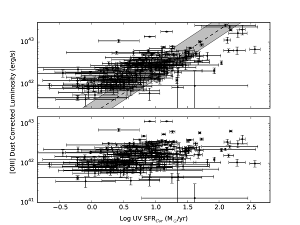
Figure 1: Top: Dust corrected UV star formation rate compared to the dust corrected [O III] $\lambda 5007$ line luminosity. The dotted line is the Ly et al. (2007) calibration and the grey band shows its uncertainty. In general, the [O III] line is not a good SFR indicator, as it is both metallicity- and ionization-parameter dependent, but we use it here as a consistency check on our UV-derived SFRs. The robust log-log slope of the relation is $0.43\pm 0.0.5$ which, given the systematics of [O III] emission, is good agreement. Bottom: The same comparison of [O III] emission to rest-frame UV flux density, prior to dust correction; this ensures that the quantities are statistically independent. As expected, the scatter in the diagram is significantly larger. The shallower slope ($0.2\pm 0.05$) is consistent with the expected correlation of extinction with star formation rate (e.g., Bouwens et al., 2009; Bauer et al., 2011)

3.3 Stellar Mass

The photometric catalog of Skelton et al. (2014) gives SED-based stellar masses for our emission-line selected galaxies, but not their associated uncertainties. Such information is critical for any analysis of continuum-faint targets, as in these objects, the photometric errors may propagate into large, asymmetric uncertainties in the derived parameters. Consequently, to infer the masses of our LAEs and oELGs, we performed our own spectral energy distribution fitting, using the Skelton et al. (2014) photometric as a base. We began by using the population synthesis models of Bruzual & Charlot (2003), as updated in 2007 with an improved treatment of the thermal-pulsating AGB phase. (Due to the generally young ages of our systems, the differences between the masses derived from the 2003 and 2007 models are minimal.) We then adopted a Salpeter (1955) initial mass function over the range $0.1\,M_{\odot}$ to $100\,M_{\odot}$, a Calzetti (2001) dust obscuration law, and the Madau (1995) prescription for absorption by intergalactic material. Since stellar abundances are poorly constrained by broadband SED measurements, we fixed the metallicity of our models to $Z=0.2\,Z_{\odot}$, which is close to the mean gas-phase oxygen abundance measured for both LAEs (Finkelstein et al., 2011; Nakajima et al., 2013; Song et al., 2014) and our comparison set of oELGs (Grasshorn Gebhardt et al., 2015). Also, because the emission lines and nebular continuum can be an important contributor to the broadband fluxes of high-redshift galaxies (e.g., Atek et al., 2011; Schaerer & de Barros, 2009), we modeled this component using the prescription of Acquaviva et al. (2011), with updated templates from Acquaviva (2012). Finally, for simplicity, we assumed that the star formation rates of our galaxies have been constant with time; at $z\sim 2$, this hypothesis is more appropriate than that of a declining SFR (e.g. Madau & Dickinson, 2014).

In keeping with these assumptions, we did not use any photometric bandpass redward of rest-frame $3.3~{}\mu$m, as in this region interstellar medium features, such as lines from polycyclic aromatic hydrocarbons (PAHs), which are not modeled by our code, may dominate. Similarly, because the Madau (1995) correction for intergalactic absorption is statistical in nature and may not alway be modeled properly, all points blueward of Ly$\alpha$ were also excluded.

To perform SED fits, we used the stellar population fitting code GalMC (Acquaviva et al., 2011), assigning as the free parameters stellar mass, reddening, and age. This Markov-chain Monte-Carlo (MCMC) program with a Metropolis-Hastings sampler is not only much more computationally efficient than traditional grid searches, but it returns more realistic errors, as it explores degeneracies between various parameters (Metropolis et al., 1953; Hastings, 1970). Upon completion, each chain was analyzed using the CosmoMC program GetDist (Lewis & Bridle, 2002), and, since multiple chains were computed for each object, the Gelman & Rubin (1992) $R$ statistic was used to test for convergence via the $R-1<0.1$ criterion (Brooks & Gelman, 1998).

As detailed by Conroy (2013), changes in the assumed initial mass function, reddening law, stellar metallicity, and the treatment of the thermal pulsing AGB phase can lead to systematic shifts of up to $\sim 0.3$ dex in the computed stellar masses of high-redshift galaxies. However, because our LAE analysis used the exact same set of assumptions as that for the oELGs, our comparison between the two galaxy populations should be valid.

3.4 Near-UV Morphology: Size, Ellipticity, and Nearest Neighbor Distance

To measure the near-UV size, morphology, and environment of our $z\sim 2$ galaxies, we used the deep F814W images of the HST CANDELS program (Grogin et al., 2011; Koekemoer et al., 2011), and the analysis techniques described in detail by Bond et al. (2009). Most of our emission line galaxies are present on these frames, though, because not all the CANDELS images have yet been released, 5 LAEs and 67 oELGs lack data. Optimally, these morphological measurements should be performed in the rest frame optical (using the F140W WFC3 filter), as this would probe a larger fraction of the galaxies’ stars. However, at this redder wavelength, the instrumental PSF is 2.5 times larger than in the rest-frame UV, making morphological measurements of small $z\sim 2$ systems that much more difficult. Moreover, though studies have found that the structural parameters of high-redshift galaxies can sometimes change when moving from the rest-frame UV to the rest-frame optical, such is usually not the case for star-forming galaxies with little dust (e.g. Conselice, 2014). As our galaxies are found via recombination lines powered by star formation, they fall under this category. Furthermore, Bond et al. (2014) showed that the near-UV and optical size measurements for LAEs do not show significant differences.

After creating cutouts around each galaxy, we performed object identifications and background subtraction using the routines found in SExtractor (Bertin & Arnouts, 1996). We then measured the angular size of each object by using the phot routine within IRAF to determine their flux-weighted centroid and magnitude through a series of circular apertures. These aperture magnitudes were used to define the galaxy’s half-light radius, with the uncertainty in the measurement being related to total flux via

$$\frac{\sigma_{r}}{r}=0.54\frac{\sigma_{f}}{f}$$ (4)

(Bond et al., 2012). The smallest half-light radius measurable via this analysis is $\sim 0.75$ kpc, or roughly twice the resolution of HST in the F814W filter.

Next, we examined object morphology to investigate the orientation of our galaxies. In disk systems, the probability of escape for Ly$\alpha$ photons should be a function of viewing angle, with face-on galaxies having lower Ly$\alpha$ optical depths than edge-on systems (see Section 4.2 for a more complete discussion). Though we cannot unambiguously determine the inclination of a galaxy at $z\sim 2$, we can derive galaxy morphologies via Galfit (Peng et al., 2002, 2010, 2011), and use the resultant ellipticities and Sérsic (1963) indices as proxies for inclination and basic morphology. Such analyses have been performed on Ly$\alpha$ emitters by a number of authors (e.g., Bond et al., 2009; Gronwall et al., 2011), with Shibuya et al. (2014a) hinting at an anti-correlation between Ly$\alpha$ equivalent width and ellipticity. We note that, while the ellipticities of large galaxies can be found via simple ellipse fitting (e.g. Weinzirl et al., 2009), the analysis of our small $z\sim 2$ systems necessitates the more careful approach of Galfit, which convolves the instrumental PSF with models of the original image. Of course, near the resolution of the instrument, ellipticity measurements will be highly uncertain, but the vast majority of our galaxies have half-light radii that more than twice this limit. Thus, our estimates of ellipticity should be reasonably robust.

Finally, to explore the effects of mergers on Ly$\alpha$ emitters, we used SExtractor to measure the distance of each emission line galaxy to its nearest projected neighbor. By examining the frequency of close pairs and the morphological shapes of Ly$\alpha$ emitters, Shibuya et al. (2014a) concluded that the merger fraction of the class was likely between 10 and 30%. However, without a control sample, Shibuya et al. (2014a) could not place this result in context. By comparing the distribution of separations for our LAEs with that for oELGs with similar masses, we can measure the relative importance of mergers for the LAE population. Moreover, because our measurement is differential in nature, our results should be relatively insensitive to the exact choice of SExtractor parameters. To select nearest neighbor galaxies, we used a range of detection thresholds (from $1.65\,\sigma$ to $2.5\,\sigma$ above the background) and required that the number of pixels above our threshold be at least five. (We report the nearest neighbor distance found using a detection threshold of $1.65\sigma$.) By modifying these numbers, we could include or exclude faint, low-significance sources which may (or may not) be real, and thereby change the absolute form of the proximity distributions. However, the relative difference between the LAE and oELG distributions remained unaffected.

The galaxies in this study have redshifts between $1.90<z<2.35$, so the exact rest-frame wavelength probed by HST’s F814W filter varies from galaxy to galaxy. However, Bond et al. (2014) demonstrated that UV morphological measurements of $z\sim 2$ systems are robust against wavelength changes. Similarly, by examining the structure of compact massive galaxies and simulating systems as small as those in our sample, Davari et al. (2014) showed that size measurements of high-redshift galaxies are generally robust. We do note that one concern with any high-redshift size measurement is that the results may be affected by cosmological surface brightness dimming (e.g., Weinzirl et al., 2011). However, previous experience with measuring the sizes of $z\sim 2$ LAEs has demonstrated that even one orbit of HST broadband data is sufficient to avoid this issue (Hagen et al., 2014).

3.5 Derived Physical Parameters: Star Formation Rate Surface Density and Specific Star Formation Rate

Our measurements of stellar mass, size, and star formation rate can be combined to form two other physical parameters which are often used to describe the physical state of galaxies. Star formation rate surface density is simply a galaxy’s total star formation rate divided by its area, and, following Malhotra et al. (2012) (who used the term star formation intensity), we define this quantity as $\Sigma_{\rm{SFR}}={\rm{SFR}}/2\pi r^{2}$, where $r$ is the half-light radius. Similarly, the specific star formation rate of a galaxy (sSFR) is simply its SFR divided by its stellar mass, and the units of this quantity, inverse time, give a measure of the system’s age. Both $\Sigma_{\rm{SFR}}$ and sSFR have been heavily used in investigations of the different types of high-redshift galaxies and their modes of star formation (Malhotra et al., 2012; Nakajima et al., 2012; Rhoads et al., 2014; Song et al., 2014). In particular, numerous authors have argued that high-redshift LAEs have some of the highest specific star formation rates in the universe (e.g., Gawiser et al., 2007; Nakajima et al., 2012), but such statements arise principally from comparisons between LAEs and higher-mass systems such as Lyman-break and $BzK$ galaxies. Our comparison to oELGs can place this conclusion in context.

4 Results

4.1 Distributions of Physical and Morphological Parameters

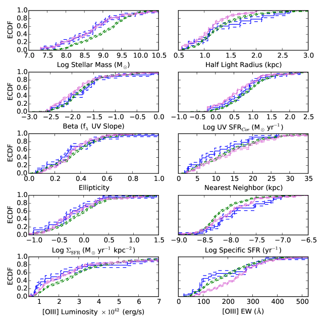
Figure 2: Empirical cumulative distribution functions (ECDFs) for 10 galaxy parameters. The solid blue line is the distribution for LAEs, while the distributions of parameters for oELGs are plotted as a green dotted line. The orchid line shows the properties of oELGs selected to match the stellar mass distribution of the LAEs. The dashed lines are the 1$\sigma$ asymptotic uncertainties. The two-sample Anderson-Darling test finds the two population are statistically identical, meaning that the null hypothesis of a single underlying population cannot be rejected for any parameter with more than 99.7% ($3\,\sigma$) confidence. The most discrepant distributions are those for stellar mass, half-light radius, and sSFR, but even those do not rise to the level of significance. The small LAE sample size means a larger difference between the two ECDFs is necessary for a significant result. We also note that the small fraction of galaxies with ellipticities greater than 0.4 suggests that at least some of the systems under consideration have disk-dominated morphologies.

Figure 2 presents the empirical cumulative distribution functions for our LAE and oELG samples, and includes the parameters stellar mass, half-light radius, stellar reddening (as measured by the slope of the UV continuum, $\beta$), star formation rate (as inferred from the de-reddened flux density at 1600 Å), ellipticity, and the projected distance to the nearest neighbor galaxy. Also shown are the cumulative distribution functions for the composite variables of $\Sigma_{\rm{SFR}}$ and specific star formation rate. Tables 1 and 2 contain all the measured physical and morphological properties for these galaxies. As illustrated in the figures, our LAEs and oELGs are drawn from consistent galactic populations: according to the Kolmogorov-Smirnov and Anderson-Darling tests, in no case can the null hypothesis of the two distributions being pulled from a single underlying population be rejected with more than 99.7% ($3\sigma$) confidence, far below the $5\sigma$ standard common in the physical sciences (Kolmogorov, 1933; Smirnov, 1948; Anderson & Darling, 1952). Our selection method for LAEs does seem to identify galaxies with slightly lower masses than their oELG counterparts, but the offset is not large and still below the threshold of statistical significance. This consistency supports the use of oELGs as an LAE comparison sample, and suggests a connection between the two galaxy populations.

To ensure that the results describe above are not an artifact of the differing depths of our LAE and oELG surveys, we created a stellar mass-matched sample of oELGs for use in our comparison. To do this, we randomly selected a mass from the LAE stellar mass distribution, applied a Gaussian uncertainty based on the error on the mass measurement, and then identified the oELG with the closest stellar mass. A total of 1,000 mass-matched oELG samples were created in this manner, and their physical and morphological properties were compared to those of the LAEs via Anderson Darling tests. As shown in Figure 2, there is no statistically significant difference between the LAEs and any of these mass-matched subsamples of optical emission line galaxies.

Another way to compare the samples while mitigating the effects of selection bias is to analyze the relationships between the various photometric and structural parameters. Since stellar mass has little to no correlation with observed Ly$\alpha$ line luminosity (Hagen et al., 2014), we treated this quantity as an independent variable, and examined the distribution of physical parameters as a function of mass for the two galaxy populations (see Figure 3). For each variable, we found the best-fit line for the oELG dataset, subtracted this line from both the oELG and LAE distributions, and compared the behavior of the residuals. In all cases, the best-fit line through the residuals had a slope consistent with zero, and there was no statistically significant difference in the distribution of the residuals. This strongly suggests that the two galaxy samples are drawn from the same underlying population. A similar analysis with half-light radius as the independent parameter produces the same result: if there is a difference between the oELG and Ly$\alpha$ emission line populations, it cannot be detected with our present samples. At least at $z\sim 2$, LAEs seem to be randomly drawn from the larger population of optical emission line galaxies.

It is somewhat surprising that the distribution of UV slopes for galaxies selected via their optical emission lines is so similar to that found for the LAE population. Many papers have suggested that Ly$\alpha$ emission is regulated by dust (e.g., Kornei et al., 2010; Atek et al., 2014, and references therein), and the existence of this dust should be revealed through extinction in the UV. Yet we see no evidence for a deficit of dust obscuration associated with Ly$\alpha$ galaxies. Of course, our analysis only addresses the global properties of each galaxy; small scale changes in the covering fraction of dust due to ISM holes created by supernovae would be extremely difficult to detect. Furthermore, the recent work by Henry et al. (2015) argues that Ly$\alpha$ emission in low-redshift Green Pea galaxies is actually modulated by H I column density. This again would weaken any supposed connection between UV extinction and Ly$\alpha$ emission.

It is also surprising that we see no significant difference between the [O III] rest-frame equivalent width (EW) distributions. The ratio of an ionization driven emission line, such as [O III] $\lambda 5007$, to its underlying starlight-generated optical or near-IR continuum is a rough proxy for specific star formation rate. Consequently, a number of authors have investigated the relationship between rest-frame optical emission-line equivalent widths and Ly$\alpha$, and have generally found a correlation between the two parameters. For example, in the nearby universe, Hayes et al. (2014) were able to select their Ly$\alpha$ Reference Sample by limiting their targets to sources with large H$\alpha$ equivalent widths, and Cowie et al. (2011) found that GALEX-selected LAEs had larger optical EWs than a control sample. Additionally, in the $z\sim 2$ universe, Oteo et al. (2015) found significant differences in the reddening, stellar mass, UV slope, and star formation rate between LAEs and a sample of H$\alpha$ selected galaxies. However, this work also found that their H$\alpha$-selected galaxies had properties similar to those of sBzK-selected systems. This suggests a simple explanation for the discrepancy: as their Figure 4 shows, their H$\alpha$ systems are systematically more massive than their Ly$\alpha$ emitters, and hence likely to be evolving along a different evolutionary path. By creating a stellar mass-matched sample of galaxies (selected primarily via their [O III] emission), we have likely avoided this problem. Alternatively, the difference between our results and those of the previous surveys could be result of the brighter Ly$\alpha$ detection limit of the HETDEX Pilot Survey. Finally, we note that our analysis is limited by small number statistics; in a few years, when large LAE samples in the HST survey fields become available, we will be able to perform much more stringent tests on the datasets.

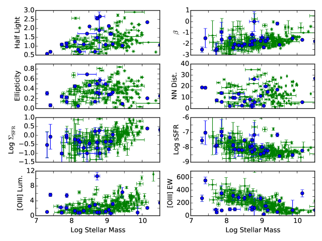
Figure 3: The physical and morphological properties of our LAE and oELGs as a function of stellar mass. LAEs (with an without rest-frame optical emission lines) are plotted as blue circles; the oELGs are plotted as green dots. The units on each quantity are the same as in Figure 2. In all cases the distributions of LAE and oELG physical parameters as a function of mass are indistinguishable; this result suggests that the two samples are drawn from the same underlying population. For stellar mass vs.  SFR, see Figure 4.

4.2 A Toy Model of the Solid Angle of Ly$\alpha$ Escape

By simulating the propagation of Ly$\alpha$ photons through a realistic ISM embedded within a $\sim 10^{10}\,M_{\odot}$ dark halo, Verhamme et al. (2012) found that the likely escape paths for Ly$\alpha$ were anisotropic, with emission much more likely along directions perpendicular to the system’s disk. In this scenario, one would expect the presence of Ly$\alpha$ to be correlated with galaxy morphology, as LAEs would be preferentially associated with low-inclination systems. Yet, as Figure 2 illustrates, no such correlation exists: the ellipticity distributions of LAEs and oELGs are statistically indistinguishable.

Alternatively, Gronke & Dijkstra (2014) and Gronke et al. (2015) have followed the escape of Ly$\alpha$ through an ISM consisting of a number of cold, dusty, star-forming clumps distributed in an hot, ionized plasma. In a case such as this, there is no preferred orientation associated with LAEs, as Ly$\alpha$ photons typically escape through low-optical depth sight lines that are randomly distributed throughout a galaxy. Indeed, there is some observational support for this idea: multiple studies have reported that when Ly$\alpha$ is observed, its optical depth is not significantly greater than that for its surrounding far-UV continuum (Finkelstein et al., 2008; Blanc et al., 2011; Hagen et al., 2014; Song et al., 2014; Vargas et al., 2014). This implies that when Ly$\alpha$ escapes, it does so without having to undergo a large number of scattering events.

If the escape of Ly$\alpha$ is indeed due to the presence of a series of randomly distributed holes in the interstellar medium, then we can use our data to determine the mean solid angle for Ly$\alpha$ emission. Of the 63 oELGs in the HPS footprint, 12 have evidence for Ly$\alpha$ in emission (Ciardullo et al., 2014), implying that $\sim 20\%$ of $z\sim 2$ star-forming galaxies have a Ly$\alpha$ escape path in our direction. If all these systems are LAEs when viewed along the appropriate line-of-sight, then the mean solid angle for Ly$\alpha$ escape is $\Omega_{Ly\alpha}=2.4\pm 0.8$ steradians. Of course, the lines-of-sight for Ly$\alpha$ escape need not be contiguous, but for purposes of visualization, this sky fraction corresponds to an average opening angle of $50^{\circ}\pm 8^{\circ}$. For comparison, a narrow-band study for $z=2.2$ star-forming galaxies in the GOODS-S region found 6 out of 55 H$\alpha$ emitting galaxies were also Ly$\alpha$ sources, for a mean escape angle of $1.4\pm 0.6$ steradians (Hayes et al., 2010). Given that this double-blind narrow-band survey covers only $\sim 5\%$ of our $1.90<z<2.35$ survey volume, and like our study, is limited by small number statistics, these results are consistent.

A further comparison comes from the analysis of Milvang-Jensen et al. (2012), who searched for Ly$\alpha$ emission from gamma-ray burst host galaxies between $1.8<z<4.5$. Recent studies suggest that GRBs at these redshifts trace UV star formation metrics (Greiner et al., 2015; Schulze et al., 2015), and as such, they provide an independent cross-check on our previous calculations. Out of a sample of 20 GRB hosts, Milvang-Jensen et al. (2012) found Ly$\alpha$ emission in 7 objects, implying a mean Ly$\alpha$ escape angle of $\Omega_{Ly\alpha}=4.4\pm 1.9$ steradians. Again, this is in rough agreement with our previous estimates.

Alternatively, we can compare our estimate of $\Omega_{Ly\alpha}$ to that obtained from the adaptive mesh radiative transfer models of Behrens & Braun (2014). These calculations follow Ly$\alpha$ transport in an isolated, turbulent disk galaxy at time steps of 1.0, 1.5, and 2.0 Gyrs after initialization. Unlike the simulations of Verhamme et al. (2012), this multiphase, dusty ISM model predicts that Ly$\alpha$ escape paths are generated stochastically, and more-or-less independent of galaxy morphology. The result seems consistent with our measurements.

To perform a more quantitative comparison, we re-analyzed the Behrens & Braun (2014) models by examining the escape of Ly$\alpha$ along 12,000 separate sight lines within the galaxy. For a galaxy to be considered an LAE, we required that the sight line have a rest-frame Ly$\alpha$ equivalent greater than 20 Å  (Gronwall et al., 2007) and an inferred Ly$\alpha$ luminosity larger than $10^{41}$ ergs s^-1 (i.e., have an intrinsic Case B star formation rate greater than $\sim 2\,M_{\odot}$ yr^-1; Hu et al., 1998; Kennicutt & Evans, 2012). The 1.5 and 2.0 Gyr models produce LAEs meeting these criteria with Ly$\alpha$ escape angles of 1.8 and 6.8 steradians, respectively. Again, this is in agreement with our observations. Interestingly, in the 1 Gyr simulation, no line of sight satisfied the observational criteria, suggesting that a more sophisticated model, such as one which includes a changing halo occupation fraction, is needed.

Finally, instead of expressing the escape of Ly$\alpha$ in terms of sight lines and opening angles, it is possible to re-parameterize the analysis into a duty cycle problem, where the time variable collectively captures all the complicated microphysics that enters into the creation of a porous ISM. Such a calculation has been performed by Chiang et al. (2015), who estimated that an LAE duty cycle of $\sim 4\%$ best fits the clustering results of the HPS survey. Of course, if our detection limits were deeper, this duty cycle estimate might increase, as more galaxies would be detected via their Ly$\alpha$ emission.

Data from the upcoming HETDEX (Hill et al., 2008) and Trident (Sandberg et al., 2015) surveys should greatly improve our understanding of Ly$\alpha$ emission from $z\sim 2$ star-forming galaxies, and allow measurements of $\Omega_{Ly\alpha}$ (or the duty cycle), as a function of stellar mass, internal reddening, and a host of other parameters. For example, it is quite possible that the factors that govern the escape of Ly$\alpha$ depend on the mass of a galaxy. In low mass systems, feedback can easily outweigh the local gravitational potential, causing the distribution of low-column density holes in the ISM to be distributed randomly and (somewhat) uniformly; this is the regime that applies to most our galaxies and to the radiative transfer models of Behrens & Braun (2014). However, in higher mass systems, the disk structure may stabilize, making it difficult to blow holes along the plane of the system. In this case, the simulations of Verhamme et al. (2012) may be more applicable. We look forward to the next generation of models detailing the kinematics of outflows through more complicated geometries which includes a multi-phase interstellar medium (e.g. Gronke & Dijkstra, 2014).

4.3 The place of LAEs and oELGs in the galaxy population

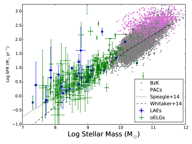
Figure 4: Galaxy star formation rate as a function of stellar mass for our sample of LAEs and oELGs. Also plotted are the continuum-selected samples of Rodighiero et al. (2011). Both LAEs and oELG systems lie along, but slightly above the low-mass extrapolation of the $z=2.1$ “main sequence” defined by Speagle et al. (2014); they also lie significantly above the Whitaker et al. (2014) main-sequence line, particularly at the low mass end. The offset could mean that the galaxies are undergoing starbursts, that there is a change in the slope of the main sequence at low stellar masses, or that that the sample is biased against low line-luminosity systems.

Figure 4 compares the star formation rates and stellar masses of our LAEs and oELGs to those of $BzK$ and Herschel-PACS galaxies (Rodighiero et al., 2011). From the figure, it is clear that the emission-line galaxies probe a mass regime that is only examined in the deepest continuum-selected surveys. Both the LAEs and oELGs do lie close to the star-forming galaxy “main sequence” (Speagle et al., 2014). However, neither population lies on the line: both sets of galaxies lie distinctly above the extrapolation of the Speagle et al. (2014) relation, and above the Whitaker et al. (2014) main sequence line.

There are several possible reasons for this offset. Perhaps the most straightforward explanation is that both galaxy populations are drawn from the same subset of high-$z$ star-bursting systems. However, another possibility is that the offset between the extrapolated main sequence and the locus of LAEs and oELGs may simply be due to errors in our estimates of stellar mass and star formation rate. Kusakabe et al. (2015) have argued that the flux densities of $z\sim 2$ LAEs are better fit using an SMC-type dust law rather than a Calzetti (2001) obscuration relation. If were to adopt such a model, our dust-corrected SFRs would move downward towards both the Speagle et al. (2014) and Whitaker et al. (2014) lines. A third reason for the discrepancy may be that a simple extrapolation of the star-forming main sequence is incorrect; it is possible that the slope of this relation changes at lower stellar mass. Finally, the higher SFRs at a given stellar mass might simply be a selection effect, as lower SFR objects are more difficult to detect through their emission lines. Larger and deeper samples of both LAEs and oELGs are required to resolve this question.

5 Conclusion

This $z\sim 2$ study finds no significant differences between the physical properties of Ly$\alpha$ emitting galaxies and galaxies selected solely by their rest-frame optical emission lines. More specifically, the distributions for LAE stellar mass, half-light radius, star formation rate, ellipticity, nearest neighbor distance, specific star formation rate, star formation rate surface density, [O III] luminosity, and [O III] equivalent width are not statistically different from those of their oELG counterparts. Surprisingly, there is not even any evidence for a difference between the two populations’ UV slopes. Since a star-forming galaxy’s spectral slope in the UV reflects the presence of dust and internal extinction, this suggests that the processes which regulate the escape of Ly$\alpha$ from a $z\sim 2$ galaxy are operating on a small scale, rather than the global scale probed by our survey. This small scale escape of Ly$\alpha$ also explains the lack of difference we found between the population’s [O III] EW and specific star formation rate distributions. It seems that the presence of Ly$\alpha$ emission in a star-forming galaxy is not a strong function of the parameters most commonly used to describe high-$z$ galaxies.

Since we have found no differences in the physical and morphological properties studies herein, the question still remains as to what causes Ly$\alpha$ to escape some galaxies and not others. As our analysis mainly concerned parameters related to stellar emission, the data would seem to suggest that at $z\sim 2$, a star-forming galaxy’s interstellar and circumgalactic media are not closely tied to the global distribution of its stars (e.g., Dijkstra et al., 2007). This matches quite well with recent observational results of both nearby LAEs and high-redshift Ly$\alpha$ halos. For example, Herenz et al. (2015) has argued that in nearby LAEs, it is the turbulence of the ISM that makes conditions favorable for Ly$\alpha$ escape. Similarly, a number of studies of Ly$\alpha$ halos surrounding $z\gtrsim 2$ star-forming galaxies have shown the extent to which the circumgalactic medium can effect Ly$\alpha$ emission (e.g., Matsuda et al., 2012; Momose et al., 2014; Wisotzki et al., 2015). Particularly intriguing are the observations of Momose et al. (2015), who found an inverse correlation between the scale length of a Ly$\alpha$ halo and the total luminosity of the Ly$\alpha$ emission. This suggests that circumgalactic conditions control whether Ly$\alpha$ is scattered out of the line of sight into a bright halo, or mostly passes through, creating an LAE. This connects well to our toy model in Section 4.2.

Though a direct comparison is not possible due sampling issues, we do note that our results are in general agreement with those of Hathi et al. (2015), who found physical similarities between LAEs and non-LAEs between $2<z<2.5$. Our results also agree with the work of Jiang et al. (2015), who found no differences in the distributions of stellar mass, age, and star formation rate for samples of $z\gtrsim 6$ LAEs and LBGs. However, our results differ from those of Cooke et al. (2010), who claimed that LBGs with small nearest neighbor separations were more likely to emit in Ly$\alpha$. One possible reason for this discrepancy is that the majority of our galaxies are much less massive than Lyman break objects: while massive galaxies might require an interaction to create an escape path for Ly$\alpha$, less organized, lower mass objects might not. Oteo et al. (2015) also found differences between the physical properties (reddening, stellar mass, and star formation rate) of $z\sim 2$ LAEs and H$\alpha$ selected systems. However, once again, this analysis does not control for stellar mass: not only is their median galaxy more than a dex larger than the systems considered here, but their Balmer-line selected galaxies are systematically more massive than their LAEs by almost a full dex. This offset in stellar mass is likely responsible for the difference in results.

While our study is limited by small number statistics, particularly with respect to the sample of LAEs, the possibility that $z\sim 2$ Ly$\alpha$ emitting galaxies are drawn from the epoch’s general star-forming population is tantalizing. Our study suggests that LAEs can be used to probe and investigate the population of low mass star forming galaxies, which, sans Ly$\alpha$ emission, are very resource intensive to identify. While this reasoning has been used to motivate LAE studies for many years, this work provides a justification for this line of attack. This hypothesis will be better tested when the HETDEX survey comes online, as commissioning data alone will generate more than a thousand LAEs in fields targeted by the HST infrared grism. This will allow a rigorous search for population differences between the LAEs and other star forming galaxies of the epoch, while controlling for stellar mass, size, and star formation rate.

Table 1: LAE Physical and Morphological Properties

RA	Dec	Log $M$	Half Light	$\beta$	Log	Ellipticity	Nearest	$\Sigma_{\rm SFR}$	Log sSFR	[O III] Lum.	[O III] EW
(2000)	(2000)	($M_{\odot}$)	(kpc)		SFRCor		Neighbor (kpc)	($M_{\odot}$ yr-1 kpc-2)	(yr-1)	$10^{41}$erg/s	Å
150.05908	2.24059	$8.52\pm 0.02$	$2.10\pm 0.02$	$-2.02\pm 0.05$	$0.99\pm 0.05$	$0.47\pm 0.03$	6.35	$0.35\pm 0.04$	$-7.52\pm 0.05$	$25.19\pm 2.96$	$275\pm 35$
150.07777	2.25000	$8.79\pm 0.13$	$1.89\pm 1.02$	$0.01\pm 0.89$	$1.62\pm 0.83$	$0.30\pm 0.08$	26.45	$1.84\pm 10.75$	$-7.17\pm 0.84$	$9.18\pm 12.02$	$122\pm 160$
150.09915	2.21952	$7.32\pm 0.01$	$0.57\pm 0.00$	$-2.50\pm 0.24$	$-0.22\pm 0.23$	$0.31\pm 0.04$	18.99	$0.29\pm 0.20$	$-7.54\pm 0.23$	$10.09\pm 1.81$	$274\pm 50$
150.11349	2.29202	$8.67\pm 0.10$	$0.69\pm 0.00$	$-2.08\pm 0.07$	$0.71\pm 0.06$	$0.14\pm 0.02$	8.26	$1.71\pm 0.28$	$-7.96\pm 0.12$	$29.46\pm 3.28$	$324\pm 39$
150.14150	2.22104	$9.06\pm 0.03$	$2.13\pm 0.01$	$-2.30\pm 0.05$	$0.68\pm 0.05$	$0.28\pm 0.03$	2.54	$0.17\pm 0.02$	$-8.38\pm 0.06$	$16.07\pm 4.26$	$22\pm 5$
150.17009	2.30639	$10.15\pm 0.00$	$2.34\pm 0.03$	$-1.63\pm 0.01$	$1.93\pm 0.01$	$0.21\pm 0.01$	5.77	$2.44\pm 0.08$	$-8.22\pm 0.01$	$21.02\pm 3.20$	$351\pm 56$
189.18378	62.23608	$9.51\pm 0.02$	–	$-2.08\pm 0.09$	$0.91\pm 0.09$	–	–	–	$-8.59\pm 0.09$	$133.73\pm 2.68$	$231\pm 12$
189.20890	62.23363	$9.87\pm 0.02$	–	$-1.49\pm 0.10$	$1.35\pm 0.09$	–	–	–	$-8.52\pm 0.09$	$8.47\pm 15.28$	$86\pm 156$
189.22592	62.22660	$7.71\pm 0.07$	–	$-2.58\pm 0.59$	$-0.21\pm 0.55$	–	–	–	$-7.92\pm 0.55$	$22.46\pm 3.23$	$94\pm 14$
189.26814	62.24616	$10.51\pm 0.01$	$1.07\pm 0.01$	$-1.76\pm 0.10$	$1.17\pm 0.09$	$0.25\pm 0.02$	27.05	$2.08\pm 0.49$	$-9.33\pm 0.09$	$34.51\pm 3.11$	$87\pm 8$
189.29592	62.19447	$8.73\pm 0.10$	–	$-2.04\pm 0.14$	$0.81\pm 0.13$	–	–	–	$-7.92\pm 0.17$	$8.93\pm 2.04$	$94\pm 22$
53.09089	-27.94874	$9.12\pm 0.06$	$1.69\pm 0.09$	$-1.73\pm 0.18$	$0.91\pm 0.17$	$0.29\pm 0.02$	19.91	$0.45\pm 0.21$	$-8.21\pm 0.18$	$6.10\pm 1.99$	$152\pm 50$
53.12923	-27.91744	$7.73\pm 0.04$	$1.09\pm 0.01$	$-2.47\pm 0.56$	$-0.14\pm 0.52$	$0.25\pm 0.03$	7.48	$0.10\pm 0.22$	$-7.87\pm 0.52$	$7.96\pm 1.86$	$51\pm 12$
53.18964	-27.89532	$9.17\pm 0.04$	$1.11\pm 0.01$	$-1.55\pm 0.22$	$0.94\pm 0.20$	$0.33\pm 0.01$	15.00	$1.10\pm 0.66$	$-8.24\pm 0.21$	$31.75\pm 4.43$	$86\pm 12$
53.06526	-27.87589	$7.41\pm 0.04$	$0.68\pm 0.00$	$-1.48\pm 0.86$	$0.39\pm 0.80$	$0.07\pm 0.03$	18.72	$0.84\pm 4.49$	$-7.02\pm 0.80$	$56.17\pm 4.55$	$552\pm 52$
53.25288	-27.85100	$8.35\pm 0.17$	$1.10\pm 0.03$	$-2.12\pm 0.41$	$0.19\pm 0.38$	–	13.20	$0.20\pm 0.28$	$-8.17\pm 0.42$	$13.24\pm 1.84$	$286\pm 42$
53.08466	-27.85090	$8.97\pm 0.10$	$1.08\pm 0.02$	$-1.74\pm 0.37$	$0.51\pm 0.35$	$0.50\pm 0.01$	11.24	$0.44\pm 0.54$	$-8.46\pm 0.36$	$10.97\pm 1.21$	$271\pm 32$
53.04775	-27.84069	$8.20\pm 0.02$	$0.81\pm 0.02$	$-2.33\pm 0.13$	$0.34\pm 0.12$	$0.05\pm 0.01$	9.78	$0.54\pm 0.17$	$-7.86\pm 0.12$	$7.65\pm 1.82$	$316\pm 76$
53.17574	-27.81654	$7.88\pm 0.02$	$0.97\pm 0.01$	$-1.60\pm 0.36$	$0.66\pm 0.34$	$0.14\pm 0.04$	6.03	$0.76\pm 0.91$	$-7.22\pm 0.34$	$54.42\pm 5.70$	$82\pm 9$
53.16744	-27.78179	$7.87\pm 0.05$	$1.16\pm 0.02$	$-0.92\pm 0.88$	$0.92\pm 0.82$	$0.23\pm 0.03$	13.97	$0.98\pm 5.42$	$-6.95\pm 0.82$	$20.83\pm 6.94$	$351\pm 118$
53.22010	-27.76466	$9.44\pm 0.02$	$1.03\pm 0.02$	$-0.17\pm 0.14$	$2.28\pm 0.13$	$0.10\pm 0.01$	16.98	$28.91\pm 10.06$	$-7.16\pm 0.13$	$63.25\pm 12.76$	$56\pm 11$
53.01713	-27.75076	$8.10\pm 0.04$	$1.25\pm 0.02$	$-1.47\pm 0.34$	$0.77\pm 0.32$	$0.45\pm 0.02$	2.32	$0.60\pm 0.64$	$-7.34\pm 0.32$	$12.93\pm 3.14$	$100\pm 24$
53.01662	-27.73105	$8.25\pm 0.16$	$0.69\pm 0.00$	$-2.03\pm 0.58$	$0.11\pm 0.54$	$1.00\pm 0.1$	9.64	$0.43\pm 1.06$	$-8.14\pm 0.57$	$7.96\pm 1.93$	$100\pm 24$
53.18055	-27.72649	$8.73\pm 0.08$	$1.48\pm 0.02$	$-1.76\pm 0.34$	$0.43\pm 0.32$	$0.50\pm 0.03$	1.70	$0.20\pm 0.21$	$-8.31\pm 0.33$	$106.39\pm 10.33$	$132\pm 14$
53.05734	-27.71681	$8.45\pm 0.26$	$1.70\pm 0.02$	$-2.18\pm 0.35$	$0.25\pm 0.33$	$0.69\pm 0.01$	2.71	$0.10\pm 0.11$	$-8.19\pm 0.42$	–	–
53.27985	-27.68197	$8.81\pm 0.14$	$2.67\pm 0.03$	$-1.67\pm 0.43$	$0.65\pm 0.40$	$0.57\pm 0.05$	5.77	$0.10\pm 0.15$	$-8.16\pm 0.42$	–	–
53.25242	-27.67421	$9.01\pm 0.07$	–	$-1.42\pm 0.24$	$1.03\pm 0.23$	–	–	–	$-7.98\pm 0.24$	–	–
53.14147	-27.67202	$8.73\pm 0.06$	$2.56\pm 0.09$	$-1.17\pm 0.28$	$1.22\pm 0.26$	$0.32\pm 0.03$	3.45	$0.40\pm 0.33$	$-7.52\pm 0.27$	–	–

Note. — Units on all the quantities are shown in the table headers. Log $M$ denotes the $\log_{10}$ stellar mass in $M_{\odot}$ assuming a Salpeter IMF, constant star formation rate, a Calzetti (2001) extinction law, and CB07 stellar population models. The half-light radius, in units of kpc, is measured in the rest-frame NUV using HST F814W images. $\beta$ is the UV spectral slope as parametrized in Equation 1. Log SFR_Cor is the $\log_{10}$ star formation rate in units of $M_{\odot}$/yr corrected using the Calzetti (2001) extinction law with reddening measured from $\beta$. Projected nearest neighbor distance is measured in kpc, using the redshift of the galaxy in question. $\Sigma_{\rm SFR}$ is dust corrected star formation rate surface density measured in units of $M_{\odot}$ yr^-1 kpc^-2. Log sSFR shows the $\log_{10}$ specific (dust-corrected) star formation rate. [O III] luminosity has also been corrected for extinction using the Calzetti (2001) law; the [O III] EW is in the rest frame, and is not dust corrected.

Table 2: oELG Physical and Morphological Properties

RA	Dec	Log $M$	Half Light	$\beta$	Log	Ellipticity	Nearest	$\Sigma_{\rm SFR}$	Log sSFR	[O III] Lum.	[O III] EW
(2000)	(2000)	($M_{\odot}$)	(kpc)		SFRCor		Neighbor (kpc)	($M_{\odot}$ yr-1 kpc-2)	(yr-1)	$10^{41}$erg/s	Å
150.06848	2.38355	$10.18\pm 0.35$	$1.21\pm 0.01$	$-1.00\pm 0.02$	$2.18\pm 0.02$	$0.11\pm 0.01$	5.85	$16.45\pm 0.84$	$-8.00\pm 0.35$	$191.70\pm 8.38$	$87\pm 5$
150.08272	2.38670	$9.32\pm 0.03$	$2.73\pm 0.07$	$-2.25\pm 0.06$	$0.70\pm 0.06$	$0.75\pm 0.01$	4.72	$0.11\pm 0.02$	$-8.62\pm 0.06$	$25.43\pm 3.79$	$199\pm 31$
150.14810	2.21751	$9.70\pm 0.01$	$1.46\pm 0.02$	$-1.25\pm 0.06$	$1.48\pm 0.05$	$0.06\pm 0.02$	13.41	$2.23\pm 0.30$	$-8.22\pm 0.05$	$54.65\pm 7.64$	$120\pm 17$
150.07210	2.32402	$9.58\pm 0.39$	$1.54\pm 0.03$	$-1.54\pm 0.06$	$1.36\pm 0.06$	$0.38\pm 0.01$	11.69	$1.51\pm 0.21$	$-8.23\pm 0.40$	$19.24\pm 4.71$	$43\pm 10$
150.08967	2.33157	$9.52\pm 0.01$	$1.27\pm 0.02$	$-1.62\pm 0.07$	$1.14\pm 0.06$	$0.41\pm 0.01$	12.89	$1.36\pm 0.22$	$-8.39\pm 0.06$	$21.90\pm 3.09$	$86\pm 12$
150.06555	2.34114	$8.25\pm 0.09$	$0.95\pm 0.04$	$-1.64\pm 0.15$	$0.73\pm 0.14$	$0.42\pm 0.03$	20.75	$0.94\pm 0.37$	$-7.53\pm 0.17$	$22.52\pm 2.40$	$263\pm 31$
150.19652	2.29569	$9.99\pm 0.00$	$1.75\pm 0.01$	$-1.62\pm 0.02$	$1.70\pm 0.02$	$0.48\pm 0.01$	22.14	$2.59\pm 0.11$	$-8.29\pm 0.02$	$101.67\pm 5.19$	$116\pm 8$
150.17356	2.30004	$9.94\pm 0.09$	$1.16\pm 0.01$	$-1.39\pm 0.03$	$1.73\pm 0.03$	$0.04\pm 0.01$	4.40	$6.27\pm 0.38$	$-8.21\pm 0.10$	$85.82\pm 5.69$	$101\pm 8$
150.17881	2.30712	$9.48\pm 0.02$	$1.05\pm 0.01$	$-1.90\pm 0.04$	$1.07\pm 0.04$	$0.23\pm 0.01$	12.53	$1.69\pm 0.17$	$-8.41\pm 0.04$	$12.71\pm 2.63$	$50\pm 10$
150.16102	2.31007	$8.62\pm 0.04$	$1.17\pm 0.03$	$-1.79\pm 0.08$	$0.80\pm 0.07$	$0.56\pm 0.01$	21.72	$0.73\pm 0.14$	$-7.82\pm 0.09$	$31.70\pm 5.60$	$277\pm 50$
150.17587	2.31348	$9.39\pm 0.02$	$1.31\pm 0.03$	$-1.85\pm 0.08$	$0.91\pm 0.07$	$0.43\pm 0.01$	13.89	$0.76\pm 0.14$	$-8.48\pm 0.08$	$33.27\pm 5.15$	$172\pm 28$
150.09134	2.26111	$8.34\pm 0.11$	$1.35\pm 0.03$	$-2.46\pm 0.11$	$0.22\pm 0.10$	$0.24\pm 0.02$	19.70	$0.14\pm 0.04$	$-8.12\pm 0.15$	$14.77\pm 2.04$	$209\pm 30$
150.08623	2.21483	$9.42\pm 0.05$	$0.93\pm 0.03$	$-1.55\pm 0.11$	$0.96\pm 0.11$	$0.43\pm 0.02$	22.25	$1.68\pm 0.47$	$-8.46\pm 0.12$	$52.18\pm 4.04$	$335\pm 30$
150.09914	2.21955	$7.32\pm 0.01$	$0.56\pm 0.03$	$-2.50\pm 0.24$	$-0.22\pm 0.23$	$0.31\pm 0.04$	18.98	$0.30\pm 0.21$	$-7.54\pm 0.23$	$10.09\pm 1.81$	$274\pm 50$
150.07175	2.22722	$9.30\pm 0.04$	$2.15\pm 0.05$	$-1.67\pm 0.09$	$1.09\pm 0.08$	$0.70\pm 0.01$	4.07	$0.42\pm 0.09$	$-8.22\pm 0.09$	$27.06\pm 3.75$	$111\pm 16$
150.07997	2.23517	$9.33\pm 0.03$	$1.26\pm 0.02$	$-1.86\pm 0.05$	$1.06\pm 0.05$	$0.32\pm 0.02$	10.48	$1.16\pm 0.14$	$-8.27\pm 0.06$	$47.72\pm 3.84$	$193\pm 18$
150.10841	2.43971	$9.85\pm 0.02$	$1.29\pm 0.01$	$-1.69\pm 0.02$	$1.51\pm 0.02$	$0.30\pm 0.01$	24.08	$3.12\pm 0.17$	$-8.34\pm 0.03$	$59.61\pm 5.77$	$93\pm 10$
150.10192	2.44912	$9.37\pm 0.08$	$2.38\pm 0.07$	$-1.73\pm 0.09$	$1.04\pm 0.08$	$0.84\pm 0.01$	1.76	$0.31\pm 0.06$	$-8.33\pm 0.11$	$33.10\pm 6.65$	$101\pm 20$
150.09980	2.44953	$8.89\pm 0.10$	$1.46\pm 0.04$	$-1.87\pm 0.08$	$0.79\pm 0.08$	$0.44\pm 0.01$	28.53	$0.46\pm 0.09$	$-8.10\pm 0.13$	$29.20\pm 5.87$	$101\pm 20$
150.17698	2.33446	$9.55\pm 0.02$	$1.34\pm 0.02$	$-1.60\pm 0.05$	$1.33\pm 0.04$	$0.40\pm 0.01$	27.75	$1.89\pm 0.20$	$-8.22\pm 0.05$	$29.95\pm 4.63$	$79\pm 12$
150.17731	2.33779	$9.36\pm 0.07$	$1.55\pm 0.04$	$-1.45\pm 0.10$	$1.12\pm 0.09$	$0.33\pm 0.03$	13.03	$0.88\pm 0.21$	$-8.24\pm 0.11$	$34.33\pm 5.30$	$79\pm 12$
150.15133	2.47150	$9.22\pm 0.08$	$1.19\pm 0.09$	$-2.12\pm 0.13$	$0.46\pm 0.12$	$0.46\pm 0.04$	24.35	$0.32\pm 0.11$	$-8.76\pm 0.15$	$20.43\pm 2.87$	$260\pm 38$
150.09839	2.26593	$9.32\pm 0.04$	$1.16\pm 0.01$	$-1.57\pm 0.05$	$1.29\pm 0.05$	$0.55\pm 0.01$	25.81	$2.33\pm 0.28$	$-8.03\pm 0.07$	$47.29\pm 7.30$	$149\pm 24$
150.12323	2.28411	$9.56\pm 0.01$	$1.14\pm 0.01$	$-1.86\pm 0.03$	$1.13\pm 0.03$	$0.32\pm 0.01$	18.94	$1.66\pm 0.12$	$-8.43\pm 0.03$	$75.82\pm 2.73$	$276\pm 17$
150.11352	2.29210	$8.68\pm 0.12$	$0.69\pm 0.02$	$-2.08\pm 0.07$	$0.71\pm 0.06$	$0.14\pm 0.02$	8.26	$1.71\pm 0.28$	$-7.97\pm 0.14$	$29.46\pm 3.28$	$324\pm 39$
150.09535	2.28722	$9.03\pm 0.08$	$0.85\pm 0.02$	$-1.71\pm 0.10$	$0.94\pm 0.09$	$0.23\pm 0.02$	12.88	$1.90\pm 0.44$	$-8.09\pm 0.12$	$51.90\pm 4.59$	$274\pm 27$
150.11090	2.28737	$8.08\pm 0.07$	$1.09\pm 0.03$	$-2.65\pm 0.11$	$0.04\pm 0.11$	$0.29\pm 0.02$	22.78	$0.15\pm 0.04$	$-8.04\pm 0.13$	$11.85\pm 3.20$	$215\pm 59$
150.12145	2.23102	$9.32\pm 0.02$	$1.56\pm 0.02$	$-1.96\pm 0.05$	$1.01\pm 0.04$	$0.32\pm 0.01$	12.52	$0.67\pm 0.07$	$-8.31\pm 0.05$	$28.16\pm 3.65$	$131\pm 18$
150.10091	2.23657	$9.72\pm 0.01$	$1.12\pm 0.01$	$-1.32\pm 0.05$	$1.52\pm 0.05$	$0.22\pm 0.01$	29.13	$4.15\pm 0.51$	$-8.20\pm 0.05$	$45.40\pm 6.82$	$89\pm 14$
150.10604	2.24106	$8.56\pm 0.16$	$0.98\pm 0.03$	$-2.17\pm 0.16$	$0.33\pm 0.15$	$0.11\pm 0.05$	10.38	$0.36\pm 0.15$	$-8.23\pm 0.22$	$23.64\pm 2.86$	$329\pm 43$
150.09754	2.24231	$8.99\pm 0.12$	$0.96\pm 0.03$	$-1.79\pm 0.14$	$0.65\pm 0.13$	$0.17\pm 0.02$	30.10	$0.77\pm 0.28$	$-8.34\pm 0.18$	$29.85\pm 2.73$	$278\pm 29$
150.09679	2.20854	$8.76\pm 0.11$	$0.82\pm 0.02$	$-2.45\pm 0.11$	$0.27\pm 0.10$	$0.29\pm 0.03$	6.76	$0.44\pm 0.12$	$-8.49\pm 0.15$	$31.23\pm 2.80$	$386\pm 39$
150.13862	2.37917	$8.13\pm 0.06$	$0.96\pm 0.02$	$-2.47\pm 0.09$	$0.19\pm 0.08$	$0.40\pm 0.02$	15.72	$0.27\pm 0.06$	$-7.94\pm 0.10$	$14.25\pm 2.03$	$266\pm 40$
150.17932	2.21977	$9.40\pm 0.02$	$1.10\pm 0.01$	$-2.22\pm 0.04$	$0.82\pm 0.04$	$0.09\pm 0.02$	14.91	$0.86\pm 0.08$	$-8.58\pm 0.04$	$49.86\pm 2.54$	$303\pm 21$
150.18666	2.23196	$9.63\pm 0.02$	$1.76\pm 0.01$	$-2.06\pm 0.02$	$1.34\pm 0.02$	$0.62\pm 0.00$	10.99	$1.12\pm 0.04$	$-8.29\pm 0.02$	$12.46\pm 2.21$	$180\pm 33$
150.18768	2.23139	$8.56\pm 0.19$	$0.86\pm 0.03$	$-2.13\pm 0.15$	$0.37\pm 0.14$	$0.32\pm 0.02$	10.48	$0.51\pm 0.19$	$-8.19\pm 0.24$	$11.73\pm 2.08$	$180\pm 33$
150.16302	2.24749	$9.90\pm 0.01$	$2.21\pm 0.02$	$-1.51\pm 0.04$	$1.57\pm 0.03$	$0.30\pm 0.01$	24.23	$1.22\pm 0.10$	$-8.32\pm 0.03$	$47.05\pm 5.01$	$64\pm 7$
150.18888	2.23938	$7.79\pm 0.05$	$0.85\pm 0.04$	$-2.45\pm 0.18$	$-0.01\pm 0.16$	$0.16\pm 0.04$	14.00	$0.22\pm 0.10$	$-7.80\pm 0.17$	$12.13\pm 1.24$	$275\pm 31$
150.15533	2.32870	$9.55\pm 0.02$	$0.91\pm 0.02$	$-1.61\pm 0.08$	$1.02\pm 0.08$	$0.23\pm 0.02$	10.69	$2.02\pm 0.41$	$-8.53\pm 0.08$	$25.48\pm 4.18$	$106\pm 18$
150.13469	2.24804	$9.19\pm 0.02$	$0.99\pm 0.01$	$-2.37\pm 0.06$	$0.57\pm 0.06$	$0.12\pm 0.01$	21.13	$0.60\pm 0.08$	$-8.62\pm 0.06$	$24.24\pm 2.30$	$217\pm 23$
150.13585	2.25997	$9.32\pm 0.02$	$1.79\pm 0.03$	$-1.87\pm 0.06$	$1.04\pm 0.05$	$0.23\pm 0.01$	27.82	$0.55\pm 0.07$	$-8.28\pm 0.06$	$38.96\pm 4.53$	$172\pm 21$
150.14200	2.26510	$10.70\pm 0.00$	$1.10\pm 0.03$	$-1.81\pm 0.13$	$0.71\pm 0.12$	$0.14\pm 0.05$	8.49	$0.67\pm 0.22$	$-9.99\pm 0.12$	$35.38\pm 3.78$	$71\pm 8$
150.15425	2.29653	$9.58\pm 0.06$	$1.36\pm 0.05$	$-2.11\pm 0.14$	$0.30\pm 0.13$	$0.18\pm 0.05$	2.45	$0.17\pm 0.06$	$-9.28\pm 0.15$	$12.22\pm 1.29$	$180\pm 21$
150.11195	2.38845	$9.69\pm 0.01$	$1.36\pm 0.03$	$-0.98\pm 0.11$	$1.49\pm 0.11$	$0.55\pm 0.01$	20.44	$2.64\pm 0.74$	$-8.20\pm 0.11$	$46.87\pm 5.47$	$111\pm 14$
150.08148	2.29891	$9.51\pm 0.01$	$2.59\pm 0.06$	$-1.84\pm 0.07$	$1.00\pm 0.07$	$0.76\pm 0.01$	19.42	$0.24\pm 0.04$	$-8.51\pm 0.07$	$38.44\pm 5.47$	$162\pm 24$
150.08045	2.30717	$8.98\pm 0.03$	$0.61\pm 0.01$	$1.58\pm 0.43$	$3.31\pm 0.40$	$0.13\pm 0.03$	11.68	$872.21\pm 1331.72$	$-5.67\pm 0.40$	$619.98\pm 147.39$	$262\pm 63$
150.05522	2.36939	$9.60\pm 0.01$	$1.02\pm 0.01$	$-1.97\pm 0.02$	$1.23\pm 0.02$	$0.15\pm 0.01$	9.09	$2.59\pm 0.15$	$-8.37\pm 0.02$	$35.55\pm 2.41$	$114\pm 9$
150.10872	2.41218	$9.36\pm 0.02$	$1.08\pm 0.03$	$-1.85\pm 0.07$	$0.94\pm 0.06$	$0.51\pm 0.02$	6.20	$1.19\pm 0.18$	$-8.41\pm 0.06$	$21.96\pm 3.95$	$126\pm 23$
53.24912	-27.69392	$7.94\pm 0.03$	$1.16\pm 0.12$	$-2.48\pm 0.32$	$-0.11\pm 0.29$	$0.35\pm 0.06$	26.12	$0.09\pm 0.09$	$-8.05\pm 0.29$	$14.70\pm 1.54$	$332\pm 38$
53.07186	-27.82070	$9.90\pm 0.01$	$1.87\pm 0.01$	$-1.33\pm 0.07$	$1.47\pm 0.07$	$0.56\pm 0.00$	16.25	$1.34\pm 0.22$	$-8.44\pm 0.07$	$44.05\pm 6.40$	$85\pm 13$
53.13528	-27.69762	$9.83\pm 0.01$	$1.34\pm 0.01$	$-1.57\pm 0.06$	$1.55\pm 0.05$	$0.34\pm 0.01$	12.98	$3.11\pm 0.39$	$-8.28\pm 0.05$	$45.13\pm 4.85$	$78\pm 9$
53.14214	-27.83269	$8.38\pm 0.04$	$1.24\pm 0.02$	$-1.75\pm 0.32$	$0.61\pm 0.30$	$0.49\pm 0.01$	8.02	$0.42\pm 0.41$	$-7.78\pm 0.30$	$37.81\pm 2.95$	$381\pm 35$
53.22949	-27.86480	$9.48\pm 0.07$	$1.19\pm 0.02$	$-1.60\pm 0.26$	$1.03\pm 0.24$	$0.31\pm 0.01$	4.83	$1.18\pm 0.88$	$-8.45\pm 0.25$	$14.02\pm 3.27$	$51\pm 12$
53.13376	-27.80791	$8.99\pm 0.02$	$1.46\pm 0.02$	$-1.64\pm 0.10$	$0.85\pm 0.10$	$0.31\pm 0.02$	4.46	$0.54\pm 0.13$	$-8.14\pm 0.10$	$28.28\pm 2.23$	$196\pm 18$
53.14352	-27.79522	$8.61\pm 0.03$	$1.15\pm 0.02$	$-2.00\pm 0.13$	$0.59\pm 0.12$	$0.36\pm 0.03$	3.25	$0.47\pm 0.15$	$-8.01\pm 0.12$	$30.56\pm 3.21$	$381\pm 44$
53.17578	-27.81656	$8.06\pm 0.36$	$0.97\pm 0.03$	$-1.94\pm 0.26$	$0.36\pm 0.25$	$0.14\pm 0.04$	6.02	$0.39\pm 0.30$	$-7.70\pm 0.44$	$15.49\pm 2.15$	$286\pm 42$
53.13813	-27.86549	$9.29\pm 0.02$	$0.90\pm 0.01$	$-2.01\pm 0.08$	$0.90\pm 0.08$	$0.17\pm 0.01$	16.59	$1.55\pm 0.30$	$-8.39\pm 0.08$	$28.03\pm 1.68$	$192\pm 15$
53.13007	-27.84289	$8.93\pm 0.05$	$1.07\pm 0.01$	$-2.29\pm 0.10$	$0.57\pm 0.10$	$0.38\pm 0.01$	6.99	$0.52\pm 0.13$	$-8.36\pm 0.11$	$27.79\pm 1.50$	$314\pm 23$
53.15059	-27.70789	$8.84\pm 0.04$	$0.69\pm 0.04$	$-1.92\pm 0.16$	$0.94\pm 0.14$	$0.32\pm 0.03$	16.17	$2.88\pm 1.16$	$-7.91\pm 0.15$	$24.95\pm 2.96$	$236\pm 30$
53.18730	-27.89793	$8.86\pm 0.06$	$2.01\pm 0.06$	$-2.12\pm 0.17$	$0.39\pm 0.16$	$0.77\pm 0.01$	3.44	$0.10\pm 0.04$	$-8.47\pm 0.17$	$10.91\pm 2.28$	$138\pm 29$
53.18976	-27.89537	$9.17\pm 0.04$	$1.11\pm 0.02$	$-1.55\pm 0.22$	$0.93\pm 0.21$	$0.33\pm 0.01$	15.01	$1.11\pm 0.67$	$-8.23\pm 0.21$	$13.75\pm 3.15$	$94\pm 22$
53.09959	-27.93800	$9.19\pm 0.11$	$1.69\pm 0.02$	$-1.22\pm 0.22$	$1.28\pm 0.20$	$0.39\pm 0.01$	16.36	$1.06\pm 0.62$	$-7.91\pm 0.23$	$29.69\pm 4.44$	$105\pm 16$
53.16297	-27.91688	$9.53\pm 0.01$	$1.58\pm 0.01$	$-2.39\pm 0.05$	$1.01\pm 0.05$	$0.36\pm 0.00$	4.75	$0.65\pm 0.07$	$-8.52\pm 0.05$	$26.99\pm 3.05$	$99\pm 12$
53.10760	-27.76926	$8.64\pm 0.03$	$1.35\pm 0.02$	$-1.56\pm 0.30$	$0.77\pm 0.28$	$0.33\pm 0.02$	2.42	$0.51\pm 0.46$	$-7.87\pm 0.28$	$27.90\pm 2.68$	$284\pm 30$
53.11179	-27.76718	$9.32\pm 0.02$	$1.39\pm 0.01$	$-1.15\pm 0.15$	$1.47\pm 0.14$	$0.39\pm 0.01$	16.76	$2.44\pm 0.95$	$-7.85\pm 0.14$	$61.83\pm 4.21$	$151\pm 12$
53.05181	-27.84883	$9.09\pm 0.04$	$1.98\pm 0.02$	$-1.71\pm 0.14$	$0.76\pm 0.13$	$0.59\pm 0.01$	5.19	$0.24\pm 0.09$	$-8.32\pm 0.14$	$12.32\pm 2.26$	$107\pm 20$
53.07551	-27.82831	$9.43\pm 0.02$	$1.49\pm 0.01$	$-1.77\pm 0.08$	$1.10\pm 0.07$	$0.34\pm 0.01$	11.36	$0.91\pm 0.16$	$-8.32\pm 0.07$	$56.46\pm 3.93$	$249\pm 21$
53.10337	-27.84163	$8.15\pm 0.04$	$0.68\pm 0.01$	$-2.02\pm 0.19$	$0.43\pm 0.18$	$0.10\pm 0.02$	9.74	$0.92\pm 0.47$	$-7.72\pm 0.18$	$20.55\pm 1.81$	$397\pm 40$
53.16832	-27.87671	$9.53\pm 0.02$	$1.74\pm 0.02$	$-1.68\pm 0.15$	$1.09\pm 0.14$	$0.42\pm 0.02$	2.87	$0.64\pm 0.25$	$-8.44\pm 0.14$	$29.32\pm 5.13$	$104\pm 18$
53.16614	-27.87466	$9.47\pm 0.01$	$0.90\pm 0.01$	$-1.77\pm 0.11$	$1.15\pm 0.11$	$0.06\pm 0.01$	6.01	$2.76\pm 0.77$	$-8.32\pm 0.11$	$27.14\pm 3.79$	$103\pm 15$
53.18917	-27.86309	$9.04\pm 0.03$	$1.05\pm 0.01$	$-2.09\pm 0.09$	$0.58\pm 0.09$	$0.54\pm 0.01$	14.81	$0.54\pm 0.12$	$-8.46\pm 0.09$	$11.01\pm 1.56$	$139\pm 20$
53.23087	-27.89474	$8.35\pm 0.13$	$1.07\pm 0.05$	$-2.48\pm 0.19$	$-0.05\pm 0.18$	$0.35\pm 0.04$	14.13	$0.13\pm 0.07$	$-8.40\pm 0.22$	$9.08\pm 1.63$	$331\pm 61$
53.24629	-27.88908	$9.33\pm 0.01$	$1.60\pm 0.01$	$-0.03\pm 0.09$	$2.56\pm 0.08$	$0.43\pm 0.01$	6.29	$22.73\pm 4.77$	$-6.77\pm 0.08$	$67.24\pm 12.81$	$53\pm 10$
53.24427	-27.88427	$8.72\pm 0.07$	$1.37\pm 0.04$	$-1.47\pm 0.22$	$1.10\pm 0.20$	$0.56\pm 0.02$	7.55	$1.08\pm 0.64$	$-7.61\pm 0.21$	$70.09\pm 8.54$	$303\pm 39$
53.01709	-27.74002	$9.64\pm 0.01$	$0.94\pm 0.00$	$-1.65\pm 0.04$	$1.63\pm 0.04$	$0.01\pm 0.01$	6.64	$7.68\pm 0.66$	$-8.01\pm 0.04$	$52.33\pm 5.48$	$82\pm 9$
53.04458	-27.72971	$9.79\pm 0.28$	$2.91\pm 0.01$	$-1.80\pm 0.05$	$1.48\pm 0.05$	$0.45\pm 0.01$	4.60	$0.57\pm 0.07$	$-8.31\pm 0.29$	$28.26\pm 6.30$	$37\pm 8$
53.04329	-27.72713	$9.61\pm 0.01$	$1.30\pm 0.01$	$-2.07\pm 0.05$	$1.15\pm 0.04$	$0.43\pm 0.00$	13.47	$1.34\pm 0.14$	$-8.46\pm 0.04$	$34.59\pm 2.52$	$135\pm 12$
53.03610	-27.71394	$9.71\pm 0.01$	$2.26\pm 0.03$	$-1.85\pm 0.12$	$1.07\pm 0.11$	$0.58\pm 0.01$	4.97	$0.36\pm 0.11$	$-8.64\pm 0.11$	$16.87\pm 5.44$	$53\pm 17$
53.01040	-27.71408	$9.92\pm 0.00$	$2.21\pm 0.01$	$-1.35\pm 0.06$	$1.69\pm 0.06$	$0.23\pm 0.01$	16.37	$1.61\pm 0.23$	$-8.23\pm 0.06$	$46.01\pm 12.22$	$58\pm 15$
53.04419	-27.76833	$8.53\pm 0.14$	$1.08\pm 0.03$	$-1.93\pm 0.83$	$0.19\pm 0.77$	$0.56\pm 0.01$	10.82	$0.21\pm 1.04$	$-8.33\pm 0.78$	$19.33\pm 4.85$	$466\pm 119$
53.03542	-27.80838	$8.32\pm 0.04$	$0.84\pm 0.01$	$-1.96\pm 0.18$	$0.51\pm 0.17$	$0.18\pm 0.03$	4.57	$0.73\pm 0.35$	$-7.81\pm 0.17$	$22.35\pm 1.91$	$336\pm 33$
53.04000	-27.79442	$9.31\pm 0.03$	$1.18\pm 0.01$	$-1.53\pm 0.22$	$0.95\pm 0.20$	$0.52\pm 0.01$	10.14	$1.01\pm 0.60$	$-8.37\pm 0.20$	$17.35\pm 2.46$	$100\pm 15$
53.02820	-27.77938	$8.39\pm 0.11$	$1.45\pm 0.07$	$-0.62\pm 0.67$	$0.85\pm 0.63$	$0.31\pm 0.06$	14.74	$0.53\pm 1.73$	$-7.54\pm 0.64$	$42.93\pm 6.16$	$389\pm 59$
53.08472	-27.86133	$9.28\pm 0.01$	$1.90\pm 0.01$	$-0.69\pm 0.07$	$2.07\pm 0.06$	$0.49\pm 0.00$	10.72	$5.14\pm 0.82$	$-7.22\pm 0.06$	$-7.43\pm 6.12$	$-13\pm-10$
53.19357	-27.84351	$9.33\pm 0.02$	$1.27\pm 0.01$	$-1.91\pm 0.09$	$0.91\pm 0.09$	$0.53\pm 0.00$	7.25	$0.80\pm 0.18$	$-8.42\pm 0.09$	$25.68\pm 2.44$	$153\pm 16$
53.21752	-27.82591	$9.37\pm 0.03$	$1.02\pm 0.02$	$-2.04\pm 0.23$	$0.60\pm 0.22$	$0.16\pm 0.02$	20.12	$0.60\pm 0.39$	$-8.77\pm 0.22$	$12.27\pm 2.65$	$98\pm 21$
53.19595	-27.82481	$9.29\pm 0.02$	$1.17\pm 0.02$	$-1.18\pm 0.23$	$1.23\pm 0.21$	$0.32\pm 0.01$	6.18	$1.95\pm 1.23$	$-8.06\pm 0.21$	$27.48\pm 4.34$	$115\pm 19$
53.19229	-27.82294	$9.00\pm 0.04$	$1.05\pm 0.01$	$-2.08\pm 0.10$	$0.59\pm 0.10$	$0.18\pm 0.01$	17.02	$0.57\pm 0.14$	$-8.41\pm 0.10$	$18.52\pm 1.78$	$202\pm 21$
53.20340	-27.81601	$9.77\pm 0.01$	$2.06\pm 0.01$	$-1.61\pm 0.06$	$1.40\pm 0.06$	$0.51\pm 0.01$	6.93	$0.94\pm 0.14$	$-8.37\pm 0.06$	$33.92\pm 4.38$	$63\pm 8$
53.18804	-27.74458	$8.17\pm 0.09$	$1.41\pm 0.07$	$-1.38\pm 0.77$	$0.56\pm 0.71$	$0.35\pm 0.04$	10.36	$0.29\pm 1.21$	$-7.61\pm 0.72$	$16.23\pm 3.86$	$316\pm 76$
53.19244	-27.73599	$9.29\pm 0.08$	$2.31\pm 0.05$	$-1.49\pm 0.13$	$1.10\pm 0.12$	$0.72\pm 0.01$	18.50	$0.38\pm 0.12$	$-8.19\pm 0.14$	$27.95\pm 6.58$	$113\pm 27$
53.18128	-27.73417	$9.03\pm 0.03$	$0.98\pm 0.01$	$-2.06\pm 0.09$	$0.77\pm 0.09$	$0.46\pm 0.01$	11.26	$0.98\pm 0.22$	$-8.25\pm 0.09$	$21.14\pm 1.48$	$211\pm 18$
53.19071	-27.72948	$8.20\pm 0.14$	$0.55\pm 0.04$	$-0.76\pm 0.76$	$1.15\pm 0.71$	$0.44\pm 0.03$	21.11	$7.51\pm 30.62$	$-7.05\pm 0.72$	$32.97\pm 6.68$	$230\pm 48$
53.18109	-27.72681	$9.67\pm 0.02$	$1.30\pm 0.02$	$-0.51\pm 0.23$	$1.82\pm 0.21$	$0.22\pm 0.01$	15.14	$6.15\pm 3.85$	$-7.85\pm 0.21$	$47.24\pm 9.53$	$56\pm 11$
53.17942	-27.72628	$9.15\pm 0.03$	$2.01\pm 0.05$	$-1.78\pm 0.18$	$0.94\pm 0.17$	$0.69\pm 0.01$	12.81	$0.34\pm 0.17$	$-8.21\pm 0.17$	$31.75\pm 6.84$	$204\pm 45$
53.18195	-27.71891	$9.30\pm 0.01$	$0.95\pm 0.01$	$-2.19\pm 0.11$	$0.76\pm 0.10$	$0.36\pm 0.01$	15.34	$1.01\pm 0.27$	$-8.55\pm 0.10$	$41.53\pm 1.76$	$297\pm 19$
53.11838	-27.71293	$10.01\pm 0.00$	$1.63\pm 0.01$	$-1.37\pm 0.07$	$1.67\pm 0.06$	$0.63\pm 0.00$	21.09	$2.80\pm 0.44$	$-8.33\pm 0.06$	$34.89\pm 6.44$	$42\pm 8$
53.10605	-27.71073	$9.14\pm 0.03$	$1.06\pm 0.03$	$-1.05\pm 0.38$	$1.09\pm 0.35$	$0.39\pm 0.02$	15.16	$1.76\pm 2.23$	$-8.05\pm 0.36$	$39.68\pm 6.29$	$189\pm 31$
53.10193	-27.70666	$9.00\pm 0.06$	$1.30\pm 0.08$	$-1.46\pm 0.71$	$0.40\pm 0.66$	$0.39\pm 0.04$	12.37	$0.24\pm 0.84$	$-8.60\pm 0.66$	$17.57\pm 3.38$	$165\pm 32$
53.09685	-27.70879	$9.31\pm 0.02$	$1.06\pm 0.01$	$-1.66\pm 0.16$	$1.05\pm 0.15$	$0.40\pm 0.01$	12.71	$1.58\pm 0.64$	$-8.27\pm 0.15$	$24.50\pm 2.52$	$127\pm 14$
53.09352	-27.80971	$9.26\pm 0.02$	$0.88\pm 0.01$	$-1.21\pm 0.15$	$1.34\pm 0.14$	$0.11\pm 0.01$	12.17	$4.58\pm 1.74$	$-7.91\pm 0.14$	$40.65\pm 10.62$	$112\pm 29$
53.09040	-27.80183	$8.61\pm 0.09$	$0.66\pm 0.02$	$-1.67\pm 0.34$	$0.46\pm 0.32$	$0.21\pm 0.02$	10.42	$1.04\pm 1.12$	$-8.15\pm 0.33$	$9.51\pm 2.17$	$203\pm 47$
53.08913	-27.79275	$8.22\pm 0.03$	$0.82\pm 0.01$	$-2.02\pm 0.15$	$0.60\pm 0.14$	$0.18\pm 0.02$	2.23	$0.93\pm 0.35$	$-7.62\pm 0.14$	$32.80\pm 2.43$	$343\pm 30$
53.08884	-27.78168	$8.92\pm 0.11$	$1.31\pm 0.01$	$-1.87\pm 0.13$	$0.73\pm 0.12$	$0.47\pm 0.02$	8.71	$0.50\pm 0.15$	$-8.19\pm 0.16$	$24.85\pm 2.31$	$229\pm 24$
53.11297	-27.77869	$8.24\pm 0.01$	$2.02\pm 0.02$	$-2.42\pm 0.08$	$0.60\pm 0.08$	$0.35\pm 0.01$	4.82	$0.15\pm 0.03$	$-7.64\pm 0.08$	$31.41\pm 2.62$	$229\pm 22$
53.14352	-27.79522	$8.60\pm 0.03$	$1.15\pm 0.02$	$-2.00\pm 0.12$	$0.59\pm 0.12$	$0.36\pm 0.03$	3.25	$0.46\pm 0.14$	$-8.02\pm 0.12$	$30.51\pm 3.21$	$381\pm 44$
53.13915	-27.78615	$8.12\pm 0.10$	$0.71\pm 0.03$	$-2.13\pm 0.84$	$-0.23\pm 0.78$	$0.07\pm 0.05$	19.49	$0.19\pm 0.94$	$-8.35\pm 0.79$	$4.74\pm 0.59$	$297\pm 39$
53.12986	-27.78225	$9.29\pm 0.02$	$1.18\pm 0.01$	$-1.63\pm 0.17$	$1.01\pm 0.16$	$0.46\pm 0.01$	15.20	$1.18\pm 0.53$	$-8.27\pm 0.16$	$25.33\pm 2.79$	$144\pm 17$
53.14781	-27.77136	$7.96\pm 0.01$	$0.94\pm 0.01$	$-1.99\pm 0.26$	$0.55\pm 0.24$	$0.30\pm 0.02$	10.08	$0.64\pm 0.47$	$-7.41\pm 0.24$	$31.10\pm 1.17$	$378\pm 23$
53.14778	-27.76562	$9.41\pm 0.04$	$1.42\pm 0.01$	$-1.73\pm 0.10$	$1.18\pm 0.09$	$0.33\pm 0.01$	9.31	$1.20\pm 0.28$	$-8.23\pm 0.10$	$23.34\pm 5.64$	$71\pm 17$
53.10372	-27.71409	$9.48\pm 0.01$	$1.64\pm 0.02$	$-1.27\pm 0.14$	$1.42\pm 0.13$	$0.50\pm 0.01$	19.63	$1.55\pm 0.56$	$-8.06\pm 0.13$	$30.27\pm 5.26$	$58\pm 10$
53.11838	-27.71293	$9.99\pm 0.03$	$1.63\pm 0.01$	$-1.37\pm 0.07$	$1.67\pm 0.06$	$0.63\pm 0.00$	21.09	$2.80\pm 0.44$	$-8.31\pm 0.07$	$34.89\pm 6.44$	$42\pm 8$
53.16881	-27.79694	$8.19\pm 0.04$	$1.57\pm 0.04$	$-1.94\pm 0.26$	$0.44\pm 0.24$	$0.45\pm 0.02$	4.06	$0.18\pm 0.13$	$-7.74\pm 0.24$	$11.71\pm 1.68$	$198\pm 30$
53.14832	-27.79594	$8.57\pm 0.05$	$0.94\pm 0.03$	$-1.48\pm 0.49$	$0.62\pm 0.45$	$0.11\pm 0.03$	4.93	$0.74\pm 1.36$	$-7.95\pm 0.46$	$6.97\pm 1.56$	$105\pm 24$
53.14352	-27.79522	$8.60\pm 0.03$	$1.15\pm 0.02$	$-1.89\pm 0.17$	$0.67\pm 0.16$	$0.36\pm 0.03$	3.25	$0.56\pm 0.24$	$-7.94\pm 0.16$	$36.40\pm 1.45$	$413\pm 26$
53.13915	-27.78615	$8.12\pm 0.10$	$0.71\pm 0.03$	$-2.11\pm 0.85$	$-0.21\pm 0.79$	$0.07\pm 0.05$	19.48	$0.19\pm 1.00$	$-8.34\pm 0.79$	$4.80\pm 0.60$	$297\pm 39$
53.18222	-27.78331	$8.96\pm 0.04$	$1.83\pm 0.05$	$-2.00\pm 0.16$	$0.65\pm 0.15$	$0.42\pm 0.02$	3.70	$0.21\pm 0.09$	$-8.32\pm 0.16$	$8.36\pm 1.60$	$89\pm 17$
53.16746	-27.78183	$7.88\pm 0.05$	$1.17\pm 0.04$	$-0.64\pm 0.92$	$1.14\pm 0.86$	$0.23\pm 0.03$	13.97	$1.60\pm 9.98$	$-6.74\pm 0.86$	$28.54\pm 3.16$	$271\pm 32$
53.14889	-27.77750	$9.76\pm 0.02$	$0.71\pm 0.01$	$-0.50\pm 0.60$	$1.36\pm 0.56$	$0.12\pm 0.02$	12.46	$7.24\pm 18.81$	$-8.40\pm 0.56$	$20.56\pm 4.17$	$38\pm 8$
53.15381	-27.76730	$9.45\pm 0.01$	$1.45\pm 0.01$	$-2.10\pm 0.05$	$1.14\pm 0.05$	$0.33\pm 0.01$	4.53	$1.04\pm 0.12$	$-8.32\pm 0.05$	$19.94\pm 3.95$	$70\pm 14$
53.14781	-27.77136	$7.96\pm 0.01$	$0.94\pm 0.01$	$-1.99\pm 0.30$	$0.54\pm 0.27$	$0.30\pm 0.02$	10.08	$0.64\pm 0.56$	$-7.42\pm 0.27$	$31.02\pm 1.17$	$378\pm 23$
188.99576	62.20455	$8.61\pm 0.05$	–	$-1.93\pm 0.16$	$0.61\pm 0.15$	–	–	–	$-7.99\pm 0.16$	$26.93\pm 1.79$	$289\pm 24$
189.00248	62.21303	$9.15\pm 0.09$	–	$-1.90\pm 0.33$	$0.56\pm 0.31$	–	–	–	$-8.60\pm 0.32$	$7.67\pm 2.15$	$61\pm 17$
189.04899	62.21538	$8.02\pm 0.06$	–	$-2.08\pm 0.44$	$0.25\pm 0.41$	–	–	–	$-7.77\pm 0.41$	$12.90\pm 2.82$	$220\pm 49$
189.06248	62.22497	$9.02\pm 0.06$	–	$-1.97\pm 0.20$	$0.64\pm 0.19$	–	–	–	$-8.38\pm 0.20$	$14.55\pm 1.80$	$167\pm 22$
189.03772	62.23307	$9.85\pm 0.01$	–	$-1.52\pm 0.06$	$1.49\pm 0.06$	–	–	–	$-8.36\pm 0.06$	$39.70\pm 2.70$	$67\pm 5$
189.02381	62.22722	$7.87\pm 0.04$	–	$-2.37\pm 0.33$	$0.15\pm 0.31$	–	–	–	$-7.73\pm 0.31$	$20.34\pm 2.99$	$324\pm 50$
189.06606	62.22381	$8.33\pm 0.12$	–	$-2.20\pm 0.30$	$0.32\pm 0.28$	–	–	–	$-8.02\pm 0.30$	$8.81\pm 1.25$	$242\pm 36$
189.06248	62.22497	$9.02\pm 0.06$	–	$-1.97\pm 0.20$	$0.64\pm 0.19$	–	–	–	$-8.39\pm 0.20$	$14.54\pm 1.80$	$167\pm 22$
189.03772	62.23307	$9.85\pm 0.01$	–	$-1.52\pm 0.06$	$1.49\pm 0.06$	–	–	–	$-8.36\pm 0.06$	$39.67\pm 2.70$	$67\pm 5$
189.08526	62.24783	$8.45\pm 0.17$	–	$-2.26\pm 0.38$	$0.05\pm 0.35$	–	–	–	$-8.40\pm 0.39$	$5.56\pm 1.05$	$170\pm 33$
189.17219	62.29881	$9.90\pm 0.01$	–	$-1.35\pm 0.07$	$1.52\pm 0.06$	–	–	–	$-8.38\pm 0.06$	$54.39\pm 7.18$	$92\pm 13$
189.22353	62.29847	$8.03\pm 0.05$	–	$-1.83\pm 0.45$	$0.40\pm 0.42$	–	–	–	$-7.63\pm 0.42$	$27.88\pm 4.80$	$385\pm 69$
189.20491	62.30445	$8.96\pm 0.07$	–	$-1.71\pm 0.15$	$0.94\pm 0.14$	–	–	–	$-8.02\pm 0.15$	$48.99\pm 7.23$	$242\pm 37$
189.21937	62.30544	$9.45\pm 0.03$	–	$-1.87\pm 0.07$	$1.16\pm 0.06$	–	–	–	$-8.29\pm 0.07$	$49.37\pm 3.89$	$165\pm 15$
189.22689	62.30773	$8.75\pm 0.07$	–	$-1.41\pm 0.27$	$0.81\pm 0.25$	–	–	–	$-7.94\pm 0.26$	$32.84\pm 4.27$	$258\pm 36$
189.24072	62.31822	$8.23\pm 0.03$	–	$-1.34\pm 0.24$	$0.89\pm 0.23$	–	–	–	$-7.34\pm 0.23$	$62.74\pm 4.06$	$399\pm 32$
189.21432	62.32324	$8.87\pm 0.07$	–	$-2.25\pm 0.19$	$0.52\pm 0.17$	–	–	–	$-8.36\pm 0.19$	$10.73\pm 2.09$	$126\pm 25$
189.26024	62.32050	$9.77\pm 0.01$	–	$-1.94\pm 0.05$	$1.19\pm 0.04$	–	–	–	$-8.57\pm 0.04$	$18.56\pm 2.28$	$49\pm 6$
189.25123	62.32082	$8.43\pm 0.13$	–	$-1.17\pm 0.43$	$0.77\pm 0.41$	–	–	–	$-7.66\pm 0.43$	$18.05\pm 3.87$	$196\pm 43$
189.23959	62.32524	$8.33\pm 0.13$	–	$-0.44\pm 0.50$	$1.26\pm 0.47$	–	–	–	$-7.07\pm 0.49$	$20.77\pm 5.83$	$245\pm 69$
189.27839	62.32653	$9.77\pm 0.01$	–	$-1.83\pm 0.06$	$1.28\pm 0.05$	–	–	–	$-8.49\pm 0.05$	$50.69\pm 3.57$	$120\pm 10$
189.27377	62.32666	$8.82\pm 0.17$	–	$-2.10\pm 0.28$	$0.37\pm 0.26$	–	–	–	$-8.45\pm 0.31$	$11.84\pm 2.06$	$199\pm 35$
189.30246	62.32795	$10.07\pm 0.01$	–	$-1.37\pm 0.05$	$1.64\pm 0.04$	–	–	–	$-8.43\pm 0.04$	$52.36\pm 7.06$	$61\pm 8$
189.30526	62.32801	$9.10\pm 0.11$	–	$-1.64\pm 0.29$	$0.50\pm 0.27$	–	–	–	$-8.60\pm 0.29$	$9.87\pm 1.87$	$133\pm 26$
189.24342	62.32965	$8.92\pm 0.19$	–	$-2.32\pm 0.50$	$-0.05\pm 0.47$	–	–	–	$-8.98\pm 0.50$	$6.38\pm 1.84$	$180\pm 52$
189.25594	62.33626	$9.33\pm 0.08$	–	$-1.47\pm 0.36$	$0.79\pm 0.34$	–	–	–	$-8.54\pm 0.35$	$26.93\pm 3.47$	$170\pm 23$
189.28220	62.33822	$8.19\pm 0.09$	–	$-2.49\pm 0.42$	$-0.02\pm 0.39$	–	–	–	$-8.21\pm 0.40$	$18.55\pm 1.36$	$334\pm 29$
189.26735	62.34506	$10.11\pm 0.07$	–	$-0.54\pm 0.44$	$1.44\pm 0.41$	–	–	–	$-8.67\pm 0.42$	$36.27\pm 6.00$	$85\pm 14$
189.32224	62.34025	$8.62\pm 0.13$	–	$-2.66\pm 0.22$	$-0.12\pm 0.20$	–	–	–	$-8.74\pm 0.24$	$13.68\pm 1.09$	$307\pm 28$
189.32373	62.34848	$8.82\pm 0.11$	–	$-2.15\pm 0.13$	$0.48\pm 0.12$	–	–	–	$-8.34\pm 0.17$	$15.59\pm 4.10$	$203\pm 54$
189.34988	62.35917	$8.58\pm 0.16$	–	$-1.97\pm 0.61$	$0.40\pm 0.57$	–	–	–	$-8.18\pm 0.59$	$14.86\pm 1.89$	$248\pm 33$
189.33272	62.36602	$7.62\pm 0.11$	–	$-1.24\pm 1.34$	$0.38\pm 1.26$	–	–	–	$-7.24\pm 1.27$	$25.23\pm 3.96$	$486\pm 80$
189.30218	62.37042	$9.04\pm 0.07$	–	$-2.24\pm 0.22$	$0.37\pm 0.20$	–	–	–	$-8.67\pm 0.21$	$11.07\pm 1.60$	$145\pm 22$
189.07819	62.17703	$9.57\pm 0.05$	–	$-1.73\pm 0.12$	$1.18\pm 0.11$	–	–	–	$-8.39\pm 0.12$	$34.24\pm 5.66$	$98\pm 16$
189.01411	62.18331	$8.73\pm 0.10$	–	$-1.94\pm 0.26$	$0.58\pm 0.24$	–	–	–	$-8.15\pm 0.26$	$20.22\pm 2.06$	$268\pm 30$
189.07820	62.17703	$9.57\pm 0.06$	–	$-1.73\pm 0.12$	$1.18\pm 0.11$	–	–	–	$-8.38\pm 0.13$	$35.94\pm 3.57$	$99\pm 11$
189.05803	62.19085	$8.06\pm 0.19$	–	$-2.22\pm 0.28$	$0.15\pm 0.26$	–	–	–	$-7.91\pm 0.32$	$6.89\pm 0.94$	$248\pm 36$
189.05556	62.19589	$8.88\pm 0.13$	–	$-1.74\pm 0.25$	$0.70\pm 0.24$	–	–	–	$-8.18\pm 0.27$	$14.58\pm 3.32$	$150\pm 35$
189.10401	62.20656	$9.08\pm 0.07$	–	$-1.56\pm 0.18$	$1.06\pm 0.17$	–	–	–	$-8.02\pm 0.18$	$25.36\pm 4.31$	$114\pm 20$
189.16919	62.21970	$9.02\pm 0.14$	–	$-1.81\pm 0.25$	$0.69\pm 0.24$	–	–	–	$-8.32\pm 0.28$	$28.01\pm 2.66$	$235\pm 25$
189.17537	62.22540	$10.53\pm 0.17$	–	$0.52\pm 0.51$	$2.10\pm 0.48$	–	–	–	$-8.43\pm 0.51$	$249.27\pm 17.80$	$143\pm 12$
189.18707	62.22655	$7.64\pm 0.11$	–	$-1.85\pm 0.44$	$0.29\pm 0.41$	–	–	–	$-7.34\pm 0.42$	$8.76\pm 1.79$	$248\pm 52$
189.14760	62.24377	$9.67\pm 0.01$	–	$-1.68\pm 0.06$	$1.37\pm 0.05$	–	–	–	$-8.30\pm 0.05$	$40.71\pm 13.69$	$99\pm 33$
189.23168	62.24741	$8.12\pm 0.11$	$2.57\pm 0.06$	$-1.85\pm 0.21$	$0.51\pm 0.20$	$0.13\pm 0.16$	21.34	$0.08\pm 0.04$	$-7.61\pm 0.22$	$8.89\pm 1.63$	$351\pm 66$
189.19774	62.25096	$8.42\pm 0.06$	$0.89\pm 0.01$	$-2.46\pm 0.20$	$0.24\pm 0.19$	$0.45\pm 0.02$	51.08	$0.35\pm 0.19$	$-8.19\pm 0.20$	$24.43\pm 1.41$	$357\pm 27$
189.22412	62.25603	$8.44\pm 0.13$	$1.27\pm 0.02$	$-2.54\pm 0.26$	$0.15\pm 0.24$	$0.52\pm 0.05$	17.16	$0.14\pm 0.10$	$-8.29\pm 0.27$	$10.05\pm 2.02$	$229\pm 47$
189.25813	62.26390	$9.58\pm 0.02$	$1.00\pm 0.01$	$-1.99\pm 0.14$	$0.86\pm 0.13$	$0.21\pm 0.03$	11.91	$1.15\pm 0.41$	$-8.72\pm 0.13$	$36.51\pm 2.47$	$172\pm 14$
189.19239	62.26434	$9.38\pm 0.02$	–	$-2.00\pm 0.04$	$1.27\pm 0.04$	–	0.88	–	$-8.12\pm 0.04$	$77.50\pm 5.79$	$208\pm 18$
189.26161	62.26430	$8.73\pm 0.08$	$1.30\pm 0.02$	$-2.29\pm 0.16$	$0.24\pm 0.15$	$0.41\pm 0.03$	26.49	$0.17\pm 0.07$	$-8.49\pm 0.17$	$9.73\pm 1.16$	$217\pm 28$
189.23716	62.27272	$9.11\pm 0.07$	$1.78\pm 0.02$	$-1.99\pm 0.12$	$0.80\pm 0.11$	$0.63\pm 0.01$	22.53	$0.31\pm 0.09$	$-8.31\pm 0.13$	$22.31\pm 2.16$	$154\pm 16$
189.25422	62.27573	$8.78\pm 0.13$	$0.59\pm 0.04$	$-1.98\pm 0.50$	$-0.09\pm 0.47$	$0.21\pm 0.08$	22.47	$0.37\pm 0.73$	$-8.87\pm 0.49$	$4.37\pm 1.35$	$198\pm 62$
189.28491	62.27583	$8.44\pm 0.11$	$0.85\pm 0.02$	$-1.60\pm 0.30$	$0.80\pm 0.28$	$0.31\pm 0.05$	2.16	$1.39\pm 1.25$	$-7.63\pm 0.30$	$30.44\pm 3.09$	$282\pm 31$
189.25994	62.27750	$9.21\pm 0.04$	$1.18\pm 0.01$	$-1.47\pm 0.12$	$1.26\pm 0.11$	$0.39\pm 0.03$	20.73	$2.06\pm 0.60$	$-7.95\pm 0.12$	$59.99\pm 8.37$	$189\pm 28$
189.26627	62.27763	$8.09\pm 0.19$	$0.31\pm 0.01$	$-2.91\pm 0.51$	$-0.67\pm 0.48$	$0.10\pm 0.06$	13.84	$0.35\pm 0.70$	$-8.75\pm 0.51$	$9.37\pm 1.21$	$408\pm 56$
189.31006	62.28404	$9.51\pm 0.04$	$3.73\pm 0.06$	$-1.44\pm 0.12$	$1.20\pm 0.11$	–	2.74	$0.18\pm 0.05$	$-8.31\pm 0.12$	$34.42\pm 5.06$	$115\pm 17$
189.30022	62.28829	$8.00\pm 0.13$	$1.01\pm 0.04$	$-2.82\pm 0.75$	$-0.45\pm 0.70$	$0.35\pm 0.07$	18.85	$0.06\pm 0.22$	$-8.45\pm 0.71$	$18.19\pm 3.59$	$497\pm 101$
189.23436	62.28846	$8.30\pm 0.17$	–	$-1.97\pm 0.22$	$0.31\pm 0.20$	–	–	–	$-7.99\pm 0.27$	$13.89\pm 1.44$	$313\pm 36$
189.29888	62.28939	$8.09\pm 0.14$	$1.34\pm 0.04$	$-2.36\pm 0.61$	$-0.06\pm 0.57$	$0.38\pm 0.10$	2.24	$0.08\pm 0.21$	$-8.15\pm 0.58$	$9.33\pm 1.92$	$313\pm 66$
189.26949	62.29079	$8.80\pm 0.08$	$1.64\pm 0.06$	$0.24\pm 0.47$	$2.17\pm 0.44$	$0.81\pm 0.01$	6.87	$8.72\pm 15.32$	$-6.63\pm 0.45$	$227.08\pm 19.43$	$751\pm 74$
189.29635	62.29415	$8.07\pm 0.05$	$1.45\pm 0.02$	$-2.08\pm 0.16$	$0.55\pm 0.15$	$0.68\pm 0.05$	4.32	$0.27\pm 0.11$	$-7.52\pm 0.16$	$20.98\pm 1.49$	$309\pm 26$
189.33446	62.29348	$9.39\pm 0.02$	$1.69\pm 0.01$	$-2.09\pm 0.07$	$0.91\pm 0.07$	$0.11\pm 0.02$	25.93	$0.45\pm 0.07$	$-8.48\pm 0.07$	$29.16\pm 1.98$	$151\pm 12$
189.34123	62.30173	$9.70\pm 0.15$	$1.90\pm 0.00$	$-1.78\pm 0.01$	$2.04\pm 0.01$	$0.56\pm 0.00$	9.29	$4.79\pm 0.13$	$-7.66\pm 0.15$	$32.30\pm 3.37$	$23\pm 2$
189.34254	62.30152	$8.58\pm 0.08$	$1.18\pm 0.03$	$-1.45\pm 0.31$	$0.90\pm 0.29$	$0.52\pm 0.02$	2.45	$0.90\pm 0.86$	$-7.69\pm 0.30$	$43.70\pm 3.95$	$251\pm 25$
189.33936	62.30858	$9.13\pm 0.04$	$1.24\pm 0.01$	$-2.19\pm 0.07$	$0.70\pm 0.06$	$0.41\pm 0.02$	8.21	$0.52\pm 0.08$	$-8.43\pm 0.08$	$27.49\pm 1.35$	$224\pm 15$
189.33991	62.30851	$9.22\pm 0.02$	$1.61\pm 0.01$	$-2.35\pm 0.06$	$0.64\pm 0.05$	$0.47\pm 0.01$	8.21	$0.27\pm 0.04$	$-8.58\pm 0.06$	$12.42\pm 1.43$	$107\pm 13$
189.28801	62.31523	$8.91\pm 0.06$	–	$-2.45\pm 0.19$	$0.32\pm 0.17$	–	–	–	$-8.59\pm 0.18$	$8.21\pm 1.35$	$109\pm 18$
189.31805	62.32235	$9.83\pm 0.01$	–	$-1.53\pm 0.06$	$1.55\pm 0.06$	–	3.75	–	$-8.29\pm 0.06$	$72.55\pm 3.55$	$114\pm 8$
189.29659	62.31574	$9.05\pm 0.06$	–	$-1.76\pm 0.18$	$0.58\pm 0.17$	–	–	–	$-8.47\pm 0.18$	$13.80\pm 1.64$	$158\pm 20$
189.40167	62.32212	$8.79\pm 0.05$	$1.20\pm 0.02$	$-1.78\pm 0.17$	$0.70\pm 0.15$	$0.48\pm 0.02$	15.20	$0.55\pm 0.23$	$-8.10\pm 0.16$	$17.60\pm 1.68$	$171\pm 18$
189.36074	62.32344	$8.76\pm 0.19$	$1.52\pm 0.04$	$-1.81\pm 0.45$	$0.40\pm 0.42$	$0.46\pm 0.07$	51.13	$0.17\pm 0.28$	$-8.36\pm 0.46$	$11.22\pm 1.80$	$180\pm 30$
189.38253	62.32442	$8.45\pm 0.15$	$0.98\pm 0.02$	$-1.99\pm 0.40$	$0.43\pm 0.37$	$0.23\pm 0.06$	49.78	$0.45\pm 0.61$	$-8.02\pm 0.40$	$14.84\pm 1.83$	$273\pm 36$
189.38390	62.32925	$9.10\pm 0.06$	$1.05\pm 0.02$	$-1.81\pm 0.27$	$0.71\pm 0.25$	$0.54\pm 0.02$	31.55	$0.74\pm 0.58$	$-8.39\pm 0.26$	$14.27\pm 2.81$	$126\pm 25$
189.39256	62.33348	$9.73\pm 0.01$	$1.36\pm 0.01$	$-1.75\pm 0.15$	$1.20\pm 0.14$	$0.38\pm 0.01$	12.98	$1.35\pm 0.53$	$-8.53\pm 0.14$	$51.47\pm 3.77$	$120\pm 10$
189.39343	62.33770	$8.97\pm 0.04$	$0.82\pm 0.01$	$-1.84\pm 0.26$	$0.87\pm 0.24$	$0.12\pm 0.03$	20.07	$1.75\pm 1.27$	$-8.10\pm 0.24$	$38.64\pm 4.69$	$227\pm 29$
189.05848	62.14314	$9.85\pm 0.01$	–	$-0.64\pm 0.08$	$2.15\pm 0.08$	–	–	–	$-7.70\pm 0.08$	$62.60\pm 6.10$	$55\pm 6$
189.12640	62.16257	$9.63\pm 0.01$	–	$-2.07\pm 0.07$	$1.00\pm 0.07$	–	–	–	$-8.63\pm 0.07$	$23.86\pm 2.97$	$88\pm 11$
189.17192	62.18768	$9.47\pm 0.02$	–	$-1.96\pm 0.12$	$0.90\pm 0.11$	–	–	–	$-8.57\pm 0.11$	$33.36\pm 3.10$	$182\pm 19$
189.22943	62.22975	$8.97\pm 0.02$	$3.52\pm 0.02$	$-2.10\pm 0.10$	$0.85\pm 0.09$	–	3.50	$0.09\pm 0.02$	$-8.11\pm 0.09$	$38.93\pm 2.56$	$214\pm 17$
189.22578	62.22663	$7.71\pm 0.07$	–	$-2.59\pm 0.59$	$-0.22\pm 0.55$	–	–	–	$-7.93\pm 0.55$	$12.29\pm 1.87$	$351\pm 56$
189.29907	62.22747	$8.92\pm 0.04$	$0.94\pm 0.01$	$-2.08\pm 0.17$	$0.33\pm 0.16$	$0.21\pm 0.03$	34.99	$0.39\pm 0.17$	$-8.59\pm 0.16$	$12.65\pm 1.29$	$227\pm 25$
189.25837	62.23863	$8.71\pm 0.17$	$1.96\pm 0.06$	$-2.21\pm 0.53$	$0.03\pm 0.49$	$0.30\pm 0.11$	34.94	$0.04\pm 0.09$	$-8.68\pm 0.52$	$8.54\pm 1.84$	$230\pm 50$
189.29665	62.24210	$8.51\pm 0.06$	$0.89\pm 0.01$	$-2.24\pm 0.24$	$0.46\pm 0.22$	$0.36\pm 0.03$	8.37	$0.58\pm 0.38$	$-8.05\pm 0.23$	$16.38\pm 1.54$	$243\pm 25$
189.26806	62.24618	$10.51\pm 0.02$	$1.08\pm 0.01$	$-1.76\pm 0.10$	$1.18\pm 0.09$	$0.26\pm 0.02$	27.04	$2.05\pm 0.48$	$-9.33\pm 0.09$	$176.06\pm 3.53$	$231\pm 12$
189.33323	62.24905	$9.21\pm 0.05$	$1.42\pm 0.01$	$-1.92\pm 0.09$	$0.96\pm 0.08$	$0.37\pm 0.02$	11.79	$0.72\pm 0.14$	$-8.25\pm 0.09$	$41.88\pm 1.81$	$218\pm 14$
189.34656	62.26064	$10.39\pm 0.01$	$0.67\pm 0.00$	$-0.43\pm 0.05$	$2.36\pm 0.04$	$0.16\pm 0.01$	13.34	$82.01\pm 8.97$	$-8.02\pm 0.05$	$196.77\pm 49.67$	$70\pm 18$
189.33931	62.27194	$9.25\pm 0.07$	$0.95\pm 0.01$	$-1.36\pm 0.16$	$1.23\pm 0.15$	$0.03\pm 0.02$	16.79	$3.01\pm 1.21$	$-8.02\pm 0.16$	$37.92\pm 3.54$	$132\pm 14$
189.11442	62.11135	$10.32\pm 0.01$	–	$-0.89\pm 0.06$	$2.13\pm 0.05$	–	–	–	$-8.19\pm 0.05$	$111.35\pm 18.62$	$57\pm 10$
189.17800	62.11557	$9.09\pm 0.07$	–	$-0.34\pm 0.15$	$2.30\pm 0.14$	–	–	–	$-6.80\pm 0.16$	$161.82\pm 34.02$	$176\pm 38$
189.12000	62.11658	$8.09\pm 0.14$	–	$-1.96\pm 0.39$	$0.06\pm 0.37$	–	–	–	$-8.03\pm 0.39$	$8.98\pm 1.14$	$236\pm 32$
189.10132	62.11879	$9.23\pm 0.04$	–	$-2.30\pm 0.14$	$0.62\pm 0.13$	–	–	–	$-8.61\pm 0.14$	$17.87\pm 1.46$	$144\pm 13$
189.14746	62.13034	$9.32\pm 0.04$	–	$-2.15\pm 0.09$	$0.99\pm 0.08$	–	–	–	$-8.32\pm 0.09$	$13.58\pm 2.22$	$64\pm 11$
189.15377	62.13209	$7.85\pm 0.03$	–	$-2.34\pm 0.20$	$0.25\pm 0.18$	–	–	–	$-7.60\pm 0.19$	$21.64\pm 1.09$	$432\pm 30$
189.17982	62.16091	$9.27\pm 0.03$	–	$-1.53\pm 0.23$	$0.84\pm 0.22$	–	–	–	$-8.42\pm 0.22$	$25.31\pm 3.37$	$185\pm 26$
189.22796	62.16110	$8.66\pm 0.04$	–	$-2.07\pm 0.10$	$0.60\pm 0.09$	–	–	–	$-8.06\pm 0.10$	$24.62\pm 1.26$	$303\pm 21$
189.25155	62.16676	$8.69\pm 0.08$	–	$-2.24\pm 0.23$	$0.41\pm 0.21$	–	–	–	$-8.28\pm 0.22$	$12.66\pm 1.34$	$217\pm 25$
189.26131	62.16966	$8.67\pm 0.06$	–	$-1.66\pm 0.16$	$0.90\pm 0.15$	–	–	–	$-7.77\pm 0.16$	$57.39\pm 2.37$	$353\pm 22$
189.22217	62.17663	$9.54\pm 0.01$	–	$-1.69\pm 0.09$	$1.02\pm 0.08$	–	–	–	$-8.52\pm 0.08$	$29.78\pm 3.43$	$134\pm 16$
189.29343	62.17652	$8.16\pm 0.09$	–	$-2.02\pm 0.57$	$0.19\pm 0.53$	–	–	–	$-7.97\pm 0.54$	$12.27\pm 2.02$	$222\pm 38$
189.27959	62.19796	$9.14\pm 0.05$	–	$-1.89\pm 0.11$	$0.93\pm 0.10$	–	–	–	$-8.21\pm 0.11$	$24.45\pm 2.86$	$145\pm 18$
189.31272	62.20915	$7.78\pm 0.05$	$1.00\pm 0.02$	$-2.23\pm 0.46$	$0.22\pm 0.43$	$0.30\pm 0.04$	23.28	$0.27\pm 0.46$	$-7.56\pm 0.43$	$7.80\pm 1.41$	$180\pm 33$
189.39515	62.21305	$9.87\pm 0.02$	$1.59\pm 0.02$	$-1.34\pm 0.17$	$1.28\pm 0.15$	$0.46\pm 0.02$	20.71	$1.19\pm 0.51$	$-8.59\pm 0.16$	$28.14\pm 7.02$	$65\pm 16$
189.39009	62.23108	$9.57\pm 0.02$	$0.75\pm 0.01$	$-1.71\pm 0.14$	$1.05\pm 0.13$	$0.30\pm 0.01$	10.82	$3.19\pm 1.08$	$-8.52\pm 0.13$	$14.93\pm 3.01$	$68\pm 14$

Note. — For details on specific measurements, please see the note in Table 1.

References

- Acquaviva (2012) Acquaviva, V. 2012, Personal Communication
- Acquaviva et al. (2011) Acquaviva, V., Gawiser, E., & Guaita, L. 2011, ApJ, 737, 47
- Adams et al. (2011) Adams, J. J., Blanc, G. A., Hill, G. J., et al. 2011, ApJS, 192, 5
- Ade et al. (2014) Ade, P. A. R., Aghanim, N., Armitage-Caplan, C., et al. 2014, A&A, 571, A16
- Akritas et al. (1995) Akritas, M. G., Murphy, S. A., & Lavalley, M. P. 1995, Journal of the American Statistical Association, 90, 170
- Anderson & Darling (1952) Anderson, T. W., & Darling, D. A. 1952, The Annals of Mathematical Statistics, 23, 193
- Astropy Collaboration et al. (2013) Astropy Collaboration, Robitaille, T. P., Tollerud, E. J., et al. 2013, A&A, 558, A33
- Atek et al. (2014) Atek, H., Kunth, D., Schaerer, D., et al. 2014, A&A, 561, A89
- Atek et al. (2011) Atek, H., Siana, B., Scarlata, C., et al. 2011, ApJ, 743, 121
- Bauer et al. (2011) Bauer, A. E., Conselice, C. J., Pérez-González, P. G., et al. 2011, MNRAS, 417, 289
- Behrens & Braun (2014) Behrens, C., & Braun, H. 2014, A&A, 572, A74
- Behrens et al. (2014) Behrens, C., Dijkstra, M., & Niemeyer, J. C. 2014, A&A, 563, A77
- Bertin & Arnouts (1996) Bertin, E., & Arnouts, S. 1996, A&AS, 117, 393
- Blanc et al. (2011) Blanc, G. A., Adams, J. J., Gebhardt, K., et al. 2011, ApJ, 736, 31
- Bond et al. (2009) Bond, N. A., Gawiser, E., Gronwall, C., et al. 2009, ApJ, 705, 639
- Bond et al. (2012) Bond, N. A., Gawiser, E., Guaita, L., et al. 2012, ApJ, 753, 95
- Bond et al. (2014) Bond, N. A., Gardner, J. P., de Mello, D. F., et al. 2014, ApJ, 791, 18
- Bouwens et al. (2009) Bouwens, R. J., Illingworth, G. D., Franx, M., et al. 2009, ApJ, 705, 936
- Bouwens et al. (2010) Bouwens, R. J., Illingworth, G. D., Oesch, P. A., et al. 2010, ApJ, 709, L133
- Brammer et al. (2012) Brammer, G. B., van Dokkum, P. G., Franx, M., et al. 2012, ApJS, 200, 13
- Brooks & Gelman (1998) Brooks, S. P., & Gelman, A. 1998, Journal of Computational and Graphical Statistics, 7, 434
- Bruzual & Charlot (2003) Bruzual, G., & Charlot, S. 2003, MNRAS, 344, 1000
- Buat et al. (2012) Buat, V., Noll, S., Burgarella, D., et al. 2012, A&A, 545, A141
- Calzetti (2001) Calzetti, D. 2001, PASP, 113, 1449
- Cassata et al. (2015) Cassata, P., Tasca, L. A. M., Le Fèvre, O., et al. 2015, A&A, 573, A24
- Chiang et al. (2015) Chiang, Y.-K., Overzier, R. A., Gebhardt, K., et al. 2015, ApJ, 808, 37
- Ciardullo et al. (2012) Ciardullo, R., Gronwall, C., Wolf, C., et al. 2012, ApJ, 744, 110
- Ciardullo et al. (2014) Ciardullo, R., Zeimann, G. R., Gronwall, C., et al. 2014, ApJ, 796, 64
- Conroy (2013) Conroy, C. 2013, ARA&A, 51, 393
- Conselice (2014) Conselice, C. J. 2014, ARA&A, 52, 291
- Cooke et al. (2010) Cooke, J., Berrier, J. C., Barton, E. J., Bullock, J. S., & Wolfe, A. M. 2010, MNRAS, 403, 1020
- Cowie et al. (2010) Cowie, L. L., Barger, A. J., & Hu, E. M. 2010, ApJ, 711, 928
- Cowie et al. (2011) —. 2011, ApJ, 738, 136
- Davari et al. (2014) Davari, R., Ho, L. C., Peng, C. Y., & Huang, S. 2014, ApJ, 787, 69
- Deharveng et al. (2008) Deharveng, J.-M., Small, T., Barlow, T. A., et al. 2008, ApJ, 680, 1072
- Dijkstra et al. (2007) Dijkstra, M., Lidz, A., & Wyithe, J. S. B. 2007, MNRAS, 377, 1175
- Erb et al. (2006) Erb, D. K., Steidel, C. C., Shapley, A. E., et al. 2006, ApJ, 647, 128
- Finkelstein et al. (2009) Finkelstein, S. L., Rhoads, J. E., Malhotra, S., & Grogin, N. 2009, ApJ, 691, 465
- Finkelstein et al. (2008) Finkelstein, S. L., Rhoads, J. E., Malhotra, S., Grogin, N., & Wang, J. 2008, ApJ, 678, 655
- Finkelstein et al. (2011) Finkelstein, S. L., Hill, G. J., Gebhardt, K., et al. 2011, ApJ, 729, 140
- Förster Schreiber et al. (2009) Förster Schreiber, N. M., Genzel, R., Bouché, N., et al. 2009, ApJ, 706, 1364
- Gawiser et al. (2006) Gawiser, E., van Dokkum, P. G., Gronwall, C., et al. 2006, ApJ, 642, L13
- Gawiser et al. (2007) Gawiser, E., Francke, H., Lai, K., et al. 2007, ApJ, 671, 278
- Gelman & Rubin (1992) Gelman, A., & Rubin, D. B. 1992, Statistical Science, 7, 457
- Giavalisco et al. (2004) Giavalisco, M., Ferguson, H. C., Koekemoer, A. M., et al. 2004, ApJ, 600, L93
- Grasshorn Gebhardt et al. (2015) Grasshorn Gebhardt, H., Zeimann, G. R., Ciardullo, R., & Hagen, A. 2015, ApJ, In Press
- Greiner et al. (2015) Greiner, J., Fox, D. B., Schady, P., et al. 2015, ApJ, 809, 76
- Grogin et al. (2011) Grogin, N. A., Kocevski, D. D., Faber, S. M., et al. 2011, ApJS, 197, 35
- Gronke et al. (2015) Gronke, M., Bull, P., & Dijkstra, M. 2015, ApJ, 812, 123
- Gronke & Dijkstra (2014) Gronke, M., & Dijkstra, M. 2014, MNRAS, 444, 1095
- Gronwall et al. (2011) Gronwall, C., Bond, N. A., Ciardullo, R., et al. 2011, ApJ, 743, 9
- Gronwall et al. (2007) Gronwall, C., Ciardullo, R., Hickey, T., et al. 2007, ApJ, 667, 79
- Guaita et al. (2010) Guaita, L., Gawiser, E., Padilla, N., et al. 2010, ApJ, 714, 255
- Hagen et al. (2014) Hagen, A., Ciardullo, R., Gronwall, C., et al. 2014, ApJ, 786, 59
- Hao et al. (2011) Hao, C.-N., Kennicutt, R. C., Johnson, B. D., et al. 2011, ApJ, 741, 124
- Hastings (1970) Hastings, W. K. 1970, Biometrika, 57, 97
- Hathi et al. (2015) Hathi, N. P., Le Fèvre, O., Ilbert, O., et al. 2015, submitted to A&A, ArXiv e-prints, arXiv:1503.01753
- Hayes et al. (2010) Hayes, M., Östlin, G., Schaerer, D., et al. 2010, Nature, 464, 562
- Hayes et al. (2014) Hayes, M., Östlin, G., Duval, F., et al. 2014, ApJ, 782, 6
- Henry et al. (2015) Henry, A., Scarlata, C., Martin, C. L., & Erb, D. 2015, ApJ, 809, 19
- Herenz et al. (2015) Herenz, E. C., Gruyters, P., Orlitova, I., et al. 2015, A&A, In Press, arXiv:1511.05406
- Hill et al. (2008) Hill, G. J., Gebhardt, K., Komatsu, E., et al. 2008, in Astronomical Society of the Pacific Conference Series, Vol. 399, Panoramic Views of Galaxy Formation and Evolution, ed. T. Kodama, T. Yamada, & K. Aoki, 115
- Hu et al. (1998) Hu, E. M., Cowie, L. L., & McMahon, R. G. 1998, ApJ, 502, L99
- Hunter (2007) Hunter, J. D. 2007, Computing in Science & Engineering, 9, 90
- Jiang et al. (2015) Jiang, L., Finlator, K., Cohen, S. H., et al. 2015, ArXiv e-prints, arXiv:1511.01519
- Jones et al. (2001) Jones, E., Oliphant, T., Peterson, P., et al. 2001, SciPy: Open source scientific tools for Python
- Kennicutt & Evans (2012) Kennicutt, R. C., & Evans, N. J. 2012, ARA&A, 50, 531
- Kennicutt (1992) Kennicutt, Jr., R. C. 1992, ApJ, 388, 310
- Kennicutt (1998) —. 1998, ARA&A, 36, 189
- Koekemoer et al. (2011) Koekemoer, A. M., Faber, S. M., Ferguson, H. C., et al. 2011, ApJS, 197, 36
- Kolmogorov (1933) Kolmogorov, A. 1933, G. Inst. Ital. Attuari, 83
- Kornei et al. (2010) Kornei, K. A., Shapley, A. E., Erb, D. K., et al. 2010, ApJ, 711, 693
- Kriek & Conroy (2013) Kriek, M., & Conroy, C. 2013, ApJ, 775, L16
- Kusakabe et al. (2015) Kusakabe, H., Shimasaku, K., Nakajima, K., & Ouchi, M. 2015, ApJ, 800, L29
- Le Fèvre et al. (2015) Le Fèvre, O., Tasca, L. A. M., Cassata, P., et al. 2015, A&A, 576, A79
- Lewis & Bridle (2002) Lewis, A., & Bridle, S. 2002, Phys. Rev. D, 66, 103511
- Ly et al. (2007) Ly, C., Malkan, M. A., Kashikawa, N., et al. 2007, ApJ, 657, 738
- Madau (1995) Madau, P. 1995, ApJ, 441, 18
- Madau & Dickinson (2014) Madau, P., & Dickinson, M. 2014, ARA&A, 52, 415
- Malhotra et al. (2012) Malhotra, S., Rhoads, J. E., Finkelstein, S. L., et al. 2012, ApJ, 750, L36
- Mannucci et al. (2009) Mannucci, F., Cresci, G., Maiolino, R., et al. 2009, MNRAS, 398, 1915
- Matsuda et al. (2012) Matsuda, Y., Yamada, T., Hayashino, T., et al. 2012, MNRAS, 425, 878
- Metropolis et al. (1953) Metropolis, N., Rosenbluth, A. W., Rosenbluth, M. N., Teller, A. H., & Teller, E. 1953, J. Chem. Phys., 21, 1087
- Milvang-Jensen et al. (2012) Milvang-Jensen, B., Fynbo, J. P. U., Malesani, D., et al. 2012, ApJ, 756, 25
- Momose et al. (2014) Momose, R., Ouchi, M., Nakajima, K., et al. 2014, MNRAS, 442, 110
- Momose et al. (2015) —. 2015, ArXiv e-prints, arXiv:1509.09001
- Moustakas et al. (2006) Moustakas, J., Kennicutt, Jr., R. C., & Tremonti, C. A. 2006, ApJ, 642, 775
- Murphy et al. (2011) Murphy, E. J., Condon, J. J., Schinnerer, E., et al. 2011, ApJ, 737, 67
- Nakajima et al. (2013) Nakajima, K., Ouchi, M., Shimasaku, K., et al. 2013, ApJ, 769, 3
- Nakajima et al. (2012) —. 2012, ApJ, 745, 12
- Nilsson et al. (2011) Nilsson, K. K., Östlin, G., Møller, P., et al. 2011, A&A, 529, A9
- Oliphant (2007) Oliphant, T. 2007, Computing in Science & Engineering, 9, 10
- Oteo et al. (2015) Oteo, I., Sobral, D., Ivison, R. J., et al. 2015, MNRAS, 452, 2018
- Ouchi et al. (2010) Ouchi, M., Shimasaku, K., Furusawa, H., et al. 2010, ApJ, 723, 869
- Pedregosa et al. (2011) Pedregosa, F., Varoquaux, G., Gramfort, A., et al. 2011, Journal of Machine Learning Research, 12, 2825
- Peng et al. (2002) Peng, C. Y., Ho, L. C., Impey, C. D., & Rix, H.-W. 2002, AJ, 124, 266
- Peng et al. (2010) —. 2010, AJ, 139, 2097
- Peng et al. (2011) —. 2011, GALFIT: Detailed Structural Decomposition of Galaxy Images, astrophysics Source Code Library, ascl:1104.010
- Pérez & Granger (2007) Pérez, F., & Granger, B. E. 2007, Computing in Science and Engineering, 9, 21
- Price et al. (2014) Price, S. H., Kriek, M., Brammer, G. B., et al. 2014, ApJ, 788, 86
- Reddy et al. (2010) Reddy, N. A., Erb, D. K., Pettini, M., Steidel, C. C., & Shapley, A. E. 2010, ApJ, 712, 1070
- Rhoads et al. (2014) Rhoads, J. E., Malhotra, S., Richardson, M. L. A., et al. 2014, ApJ, 780, 20
- Rodighiero et al. (2011) Rodighiero, G., Daddi, E., Baronchelli, I., et al. 2011, ApJ, 739, L40
- Salpeter (1955) Salpeter, E. E. 1955, ApJ, 121, 161
- Sandberg et al. (2015) Sandberg, A., Guaita, L., Östlin, G., Hayes, M., & Kiaeerad, F. 2015, A&A, 580, A91
- Schaerer & de Barros (2009) Schaerer, D., & de Barros, S. 2009, A&A, 502, 423
- Schaerer et al. (2011) Schaerer, D., Hayes, M., Verhamme, A., & Teyssier, R. 2011, A&A, 531, A12
- Schulze et al. (2015) Schulze, S., Chapman, R., Hjorth, J., et al. 2015, ApJ, 808, 73
- Scoville et al. (2007) Scoville, N., Aussel, H., Brusa, M., et al. 2007, ApJS, 172, 1
- Sérsic (1963) Sérsic, J. L. 1963, Boletin de la Asociacion Argentina de Astronomia La Plata Argentina, 6, 41
- Shibuya et al. (2014a) Shibuya, T., Ouchi, M., Nakajima, K., et al. 2014a, ApJ, 785, 64
- Shibuya et al. (2014b) —. 2014b, ApJ, 788, 74
- Shivaei et al. (2015) Shivaei, I., Reddy, N. A., Steidel, C. C., & Shapley, A. E. 2015, ApJ, 804, 149
- Skelton et al. (2014) Skelton, R. E., Whitaker, K. E., Momcheva, I. G., et al. 2014, ApJS, 214, 24
- Smirnov (1948) Smirnov, N. 1948, The Annals of Mathematical Statistics, 19, 279
- Song et al. (2014) Song, M., Finkelstein, S. L., Gebhardt, K., et al. 2014, ApJ, 791, 3
- Speagle et al. (2014) Speagle, J. S., Steinhardt, C. L., Capak, P. L., & Silverman, J. D. 2014, ApJS, 214, 15
- Steidel et al. (1996a) Steidel, C. C., Giavalisco, M., Dickinson, M., & Adelberger, K. L. 1996a, AJ, 112, 352
- Steidel et al. (1996b) Steidel, C. C., Giavalisco, M., Pettini, M., Dickinson, M., & Adelberger, K. L. 1996b, ApJ, 462, L17
- Storey & Zeippen (2000) Storey, P. J., & Zeippen, C. J. 2000, MNRAS, 312, 813
- Vargas et al. (2014) Vargas, C. J., Bish, H., Acquaviva, V., et al. 2014, ApJ, 783, 26
- Verhamme et al. (2012) Verhamme, A., Dubois, Y., Blaizot, J., et al. 2012, A&A, 546, A111
- Verhamme et al. (2006) Verhamme, A., Schaerer, D., & Maselli, A. 2006, A&A, 460, 397
- Weiner et al. (2014) Weiner, B. J., et al. 2014, in American Astronomical Society Meeting Abstracts, Vol. 223, American Astronomical Society Meeting Abstracts #223, #227.07
- Weinzirl et al. (2009) Weinzirl, T., Jogee, S., Khochfar, S., Burkert, A., & Kormendy, J. 2009, ApJ, 696, 411
- Weinzirl et al. (2011) Weinzirl, T., Jogee, S., Conselice, C. J., et al. 2011, ApJ, 743, 87
- Whitaker et al. (2014) Whitaker, K. E., Franx, M., Leja, J., et al. 2014, ApJ, 795, 104
- Wisotzki et al. (2015) Wisotzki, L., Bacon, R., Blaizot, J., et al. 2015, ArXiv e-prints, arXiv:1509.05143
- Wuyts et al. (2013) Wuyts, S., Förster Schreiber, N. M., Nelson, E. J., et al. 2013, ApJ, 779, 135
- Yajima et al. (2012) Yajima, H., Li, Y., Zhu, Q., et al. 2012, ApJ, 754, 118
- Zeimann et al. (2014) Zeimann, G. R., Ciardullo, R., Gebhardt, H., et al. 2014, ApJ, 790, 113
- Zeimann et al. (2015) Zeimann, G. R., Ciardullo, R., Gronwall, C., et al. 2015, ApJ, in press, arXiv:1511.00651