Antiproton–proton annihilation into pion pairs within effective meson theory

Abstract

Antiproton–proton annihilation into light mesons is revisited in the few GeV energy domain, in view of a global description of the existing data. An effective meson model is developed, with mesonic and baryonic degrees od freedom in $s$, $t$, and $u$ channels. Regge factors are added to reproduce the proper energy behavior and the forward and backward peaked behavior. A comparison with existing data and predictions for angular distributions and energy dependence are done for charged and neutral pion pair production.

Physics Letters B PLB Physics Letters B 2011Published by Elsevier Ltd.

1 Introduction

Large experimental and theoretical efforts have been going on since decades in order to understand and classify high energy processes driven by strong interaction. We revisit here hadronic reactions at incident energies above 1 GeV, focusing on two body processes.

Antiprotons are a very peculiar probe, due to the fact that scattering and annihilation may occur in the same process, with definite kinematical characteristics. We discuss the annihilation reaction of antiproton-proton into two charged or neutral pions and the crossed channels of pion-proton elastic scattering. These reactions have been studied in the past, mostly at lower energies, in connection with data from LEAR and FermiLab (for a review, see [1]). At low energies the annihilation into light meson pairs is dominated by few partial waves and the angular distributions show a series of oscillations. Data are usually given in terms of Legendre polynomials. This regime was studied with the aim to look for resonances in the $\bar{p}p$ system. A change of behavior appears around $\sqrt{s}$=2 GeV where two body processes become mostly peripheral. They are peaked forward or backward, corresponding to small values of $t$ or $u$, respectively ($s$, $t$ and $u$ are standard kinematical Mandelstam variables of binary process). The differential cross section at large momentum transfer and the integrated cross section show a power-law behavior as a function of the energy. At larger energies, the total cross section becomes asymptotically constant and reaches a regime where $d\sigma/dt$ is function only of $t$ and is independent on $s$.

The most exhaustive data on neutral pion (and other neutral meson) production have been published by the FermiLab E760 collaboration in the energy range ($2.2\leq\sqrt{s}\leq 4.4$) GeV[2]. Charged pion production data are scarce, and do not fill with continuity a large angular or energy range [3, 4, 5]. According to the foreseen performances of the experiment PANDA at FAIR, a large amount of data related to light meson pairs production from $\bar{p}p$ annihilation is expected in next future. The best possible knowledge of light meson production is also requested prior to the experiment, as pions constitute an important background for many other channels making timely the development of a reliable model.

Few calculations exist in the literature. A baryon ($N$ and $\Delta$) $t$-channel exchange model was developed by [6] with applicability below 1 GeV beam momentum. A model was recently developed at larger energies, including meson exchanges in $s-$channel, which qualitatively reproduces selected sets of angular distributions [7]. However, the authors warns against application to neighboring energies, eventually related to a specific extrapolation of Regge trajectories in the region $t<0$.

We develop here a model with meson and baryon exchanges in $s$, $t$, and $u$ channels, applicable in the energy range ($2\leq\sqrt{s}\leq 5.5$) GeV , that is the accessible domain for the PANDA experiment at FAIR. It is known that first order Born diagrams give cross sections much larger than measured, as Feynman diagram assume point-like particles. Form factors are added in order to take into account the composite nature of the interacting particles at vertexes. Their form is, however, somehow arbitrary, and parameters as coupling constants or cutoff are adjusted to reproduce the data. A ”Reggeization” of the trajectories is added to reproduce the very forward and very backward scattering angles. Therefore this class of models should be considered as an effective way to take into account microscopic degrees of freedom and quark exchange diagrams.

Our aim is to build a model with minimal ingredients, to calculate the basic features of neutral and charged pion production in the energy range that will be investigated by the future experiment PANDA at FAIR. To get maximum profit from the available data, we consider also existing $\pi^{\pm}p$ elastic scattering data, and apply crossing symmetry in order to compare the predictions based on the annihilation channel, at least in a limited kinematical range. The main requirement is that the model should be able to reproduce charged and neutral pion production from annihilation, and $\pi^{\pm}p$ elastic scattering without readjustment of the parameters.

2 Formalism

2.1 Kinematics and cross section

We consider the annihilation reaction:

$$\bar{p}(p_{1})+p(p_{2})\to\pi^{-}(k_{1})+\pi^{+}(k_{2}).$$ (1)

in the center of mass system (CMS). The notation of four momenta is shown in the parenthesis. The following notations are used: $q_{t}=(-p_{1}+k_{1})$, $q_{t}^{2}=t$, $q_{u}=(-p_{1}+k_{2})$, $q_{u}^{2}=u$ and $q_{s}=(p_{1}+p_{2})$, $q_{s}^{2}=s$, $s+t+u=2M_{N}^{2}+2m_{\pi}^{2}$, $M_{N}$($m_{\pi}$) is the nucleon(pion) mass. The useful scalar product between four vectors are explicitly written as:

$$2p_{1}k_{2}=2k_{1}p_{2}=M_{N}^{2}+m_{\pi}^{2}-u,\ 2p_{1}k_{1}=2k_{2}p_{2}=M_{N}^{2}+m_{\pi}^{2}-t,$$ (2)

$$2p_{1}p_{2}=s-2M_{N}^{2},\ 2k_{1}k_{2}=s-2m_{\pi}^{2},$$

$$p_{1}^{2}=p_{2}^{2}=M_{N}^{2}=E^{2}-|\vec{p}|^{2},\ k_{1}^{2}=k_{2}^{2}=m_{\pi}^{2}=\varepsilon^{2}-|\vec{k}|^{2}.\$$

The general expression for the differential cross section in the CMS of reaction (1) is:

$$\frac{d\sigma}{d\Omega}=\displaystyle\frac{1}{2^{8}\pi^{2}}\displaystyle\frac{1}{s}\displaystyle\frac{\beta_{\pi}}{\beta_{p}}|\overline{\cal M}|^{2},\ \ \displaystyle\frac{d\sigma}{d\cos\theta}=2E^{2}\beta_{p}\beta_{\pi}\displaystyle\frac{d\sigma}{dt},$$ (3)

where ${\cal M}$ is the amplitude of the process, $\beta_{p}$($\beta_{\pi})$ is the velocity and $E(\varepsilon)$ is the energy of the proton(pion) in CMS. The phase volume can be transformed as $d\Omega\to 2\pi\ d\!\cos\theta$ due to the azimuthal symmetry of binary reactions. The total cross section is :

$$\sigma=\int\frac{|\overline{\cal M}|^{2}}{64\pi^{2}s}\frac{|\vec{p}|}{|\vec{k}|}d\Omega,$$ (4)

where $|\vec{p}|$ and $|\vec{k}|$ are the initial and final momenta (moduli) in CMS.

2.2 Crossing symmetry

Crossing symmetry relates annihilation and scattering cross sections. Crossing symmetry states that the amplitudes of the crossed processes are the same. This means that the matrix element ${\cal M}(s,t)$ is the same at corresponding $s$ and $t$ values, but the variables span different regions of the kinematical space. In order to find this correspondence, kinematical replacements between variables should be done, as indicated in Table 1. Note that the coefficients 1/2 and 1/4 in the cross section formulas are the spin factors: $(2S_{\pi}+1)(2S_{p}+1)$ and $(2S_{\bar{p}}+1)(2S_{p}+1)$ for the scattering and annihilation channels, respectively, where $S_{\pi}$, $S_{p}$ and $S_{\bar{p}}$ are the spin moduli of the corresponding initial particles. The incident momentum in the annihilation channel, corresponding to the invariant $s$ is: $|\vec{p}_{a}|=\sqrt{{s}/{4}-M^{2}}$. From the equality $s_{a}=s_{s}$, the CMS momentum for $\pi^{-}p$ scattering, $|k_{s}|$, is evaluated at the same $s$ value:

$$|\vec{k}_{s}|^{2}=\displaystyle\frac{1}{4s}\left[m^{4}-2m^{2}(M^{2}+s)+(M^{2}-s)^{2}\right].$$ (5)

Then the cross sections for the two crossed processes are related by:

$$\sigma^{a}=\displaystyle\frac{1}{2}\displaystyle\frac{|\vec{k}_{s}|^{2}}{|\vec{p}_{a}|^{2}}\sigma^{s}.$$ (6)

If the scattering cross section is measured at a value $s^{s}=s_{1}$ different from $s^{a}=s$, at small $t$ values one may rescale the cross section, using the empirical dependence: $\sigma^{s}\simeq const\cdot s^{-2}$.

Annihilation	Scattering
$\bar{p}(p_{1})+p(p_{2})\to\pi^{-}(k_{1})+\pi^{+}(k_{2})$	$\pi^{-}(-k_{2})+p(p_{2})\to\pi^{-}(k_{1})+p(-p_{1})$
$s_{a}=(p_{1}+p_{2})^{2}$	$s_{s}=(-k_{2}+p_{2})^{2}$
$t_{a}=(p_{1}-k_{1})^{2}$	$t_{s}=(-k_{2}-k_{1})^{2}$
$u_{a}=(p_{1}-k_{2})^{2}$	$u_{s}=(p_{1}-k_{2})^{2}$
$s_{a}=4E^{2}=4(M^{2}+|\vec{p}_{a}|^{2})$	$s_{s}=m^{2}+M^{2}+2E_{2}^{\prime}\epsilon_{2}^{\prime}+2|k_{s}|^{2}$
$\sigma^{(a)}=\displaystyle\frac{1}{4}\displaystyle\frac{|{\cal M}_{(a)}|^{2}}{64\pi^{2}s}\displaystyle\frac{|\vec{k_{a}}|}{|\vec{p_{a}}|}$	$\sigma^{(s)}=\displaystyle\frac{1}{2}\displaystyle\frac{|{\cal M}_{(s)}|^{2}}{64\pi^{2}s}\displaystyle\frac{|\vec{k}_{s}|}{|\vec{p}_{s}|}$

Table 1: Correspondence between variables in the crossed scattering (s) and annihilation (a) channels.

3 Formalism

The formulas written above are model independent, i.e., they hold for any reaction mechanism. In order to calculate ${\cal M}$, one needs to specify a model for the reaction. In this work we consider the process (1) within the formalism of effective meson lagrangians.

The following contributions to the cross section for reaction (1) are calculated, as illustrated in Fig. (1):

• baryon exchange:

  • $t$-channel nucleon (neutron) exchange, Fig. 1.a,

  • $t$-channel $\Delta^{0}$ exchange, Fig. 1.b,

  • $u$-channel $\Delta^{++}$ exchange , Fig. 1c;

• $s$-channel $\rho$-meson exchange, Fig. 1d.

The total amplitude is written as a coherent sum of all the amplitudes:

$${\cal M}={\cal M}_{n}+{\cal M}_{\Delta^{0}}+{\cal M}_{\Delta^{++}}+{\cal M}_{\rho}.$$ (7)

In case of charged pions, the dominant contribution in forward direction is $N$ exchange, whereas $\Delta^{++}$ mostly contribute to backward scattering. We neglect the difference of masses between the nucleons as well as between different charge states of the pion and of the $\Delta$. Large angle scattering is driven by s-channel exchange of vector mesons, with the same quantum numbers as the photon. We limit our considerations to $\rho$-meson exchange.

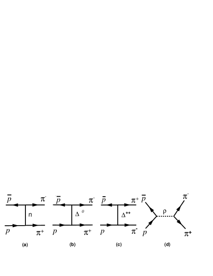
Figure 1: Feynman diagrams for the reaction $\bar{p}+p\to\pi^{-}+\pi^{+}$ within effective meson Lagrangian approach.

The expressions for the amplitudes and their interferences are detailed in the Appendix. Coupling constants are fixed from the known decays of the particles if it is possible, otherwise we use the values from effective potentials as [20]. Masses and widths are taken from [21].

The effects of strong interaction in the initial state coming from the exchange by vector and (pseudo)scalar mesons between proton-antiproton are essential and effectively lead to the Regge form of the amplitude. The $t$ and $u$ diagrams are modified by adding a general Regge factor $R_{x}$ (where $x=t,u$) with the following form:

$$R(x)=\left(\displaystyle\frac{s}{s_{0}}\right)^{2[\alpha(x)-1]},~{}\alpha(x)=\displaystyle\frac{1}{2}+r\displaystyle\frac{\alpha_{s}}{\pi}\displaystyle\frac{x-M^{2}}{M^{2}};$$ (8)

where $s_{0}\simeq 1$ GeV² can be considered a fitting parameter [22] and $r\alpha_{s}/\pi\simeq 0.7$ is fixed by the slope of the Regge trajectory. In the present model the values have been set at $s_{0}=1.4$ GeV² and $r\alpha_{s}/\pi=0.7$ for the nucleon.

This Regge form of amplitude incorporates in principle infinite number of resonances, (i.e. $\Delta(1232)$ and others). The trajectory for the $\Delta$ resonance is known to be different from the nucleon. The slope parameter is fixed in this case as $r\alpha_{s}/\pi=1.4$. As for excited resonances like $N^{*}\left(1440\right)$ they belong to a daughter Regge trajectory which is power suppressed compared to the leading one. Omitting these contributions involves an estimated uncertainty of 10%.

A form factor of the form:$F=1/(x-p^{2}_{N,\Delta})^{2}$, was introduced in the $Np\bar{p}$ and $Np\bar{\Delta}$ vertexes, with $p_{N}=0.8$ GeV and $p_{\Delta}$ =5 GeV.

The $\rho NN$ vertex includes the proton structure in the vector current form with two form factors (FF) $F_{1,2}^{\rho}$:

$$\Gamma_{\mu}(q_{s})=F_{1}^{\rho}(q_{s}^{2})\gamma_{\mu}(q_{s})+\displaystyle\frac{i}{2M_{N}}F_{2}^{\rho}(q_{s}^{2}),\sigma_{\mu\nu}q_{s}^{\nu},$$ (9)

where $\sigma_{\mu\nu}=\displaystyle\frac{i}{2}[\gamma_{\mu}\gamma_{\nu}-\gamma_{\nu}\gamma_{\mu}]$ is the antisymmetric tensor. Due to the isovector nature of the $\rho$, the $\rho NN$ is similar to the electromagnetic vertex $\gamma NN$. However the two form factors $F_{1,2}^{\rho}(q_{s}^{2})$ are different from the proton electromagnetic ones. Due to the freedom of the choice, we do not attempt any rearrangement, but prefer to fix the form, the constants and the parameters of $F_{1,2}^{\rho}(s)$ according to [23, 24, 20] as:

$$F_{1}^{\rho}(s)=g_{\rho NN}\frac{\Lambda^{4}}{\Lambda^{4}+(s-M_{\rho}^{2})^{2}},\qquad F_{2}^{\rho}(s)=\kappa_{\rho}F_{1}^{\rho}(s),$$ (10)

with normalization $F_{1}^{\rho}(M_{\rho}^{2})=g_{\rho NN}$, where the constant $g_{\rho NN}$ corresponds to the coupling of the vector meson $\rho$ with the nucleon ($g^{2}_{\rho NN}/(4\pi)=0.55$) , $\kappa_{\rho}=3.7$ is the anomalous magnetic moment of the proton with respect to the coupling with $\rho$, and $\Lambda=0.911$ is an empirical cut-off.

To take into account the composite nature of the pion, in principle, a monopole type $\rho\pi\pi$ form factor may be introduced: $F_{\rho\pi\pi}=A_{\pi}/{(s-A_{\pi})}^{2}$, where $A_{\pi}$ is a parameters to be adjusted on the data. In the present case $F_{\rho\pi\pi}$ was set to one.

The diagrams for neutral pion pair production are illustrated in Fig. 2 , where we consider proton and $\Delta^{+}$ exchange in $t-$channel and $\rho$-meson exchange in $s-$ channel. The calculated amplitudes are symmetrized, to take into account the identity of the final particles.

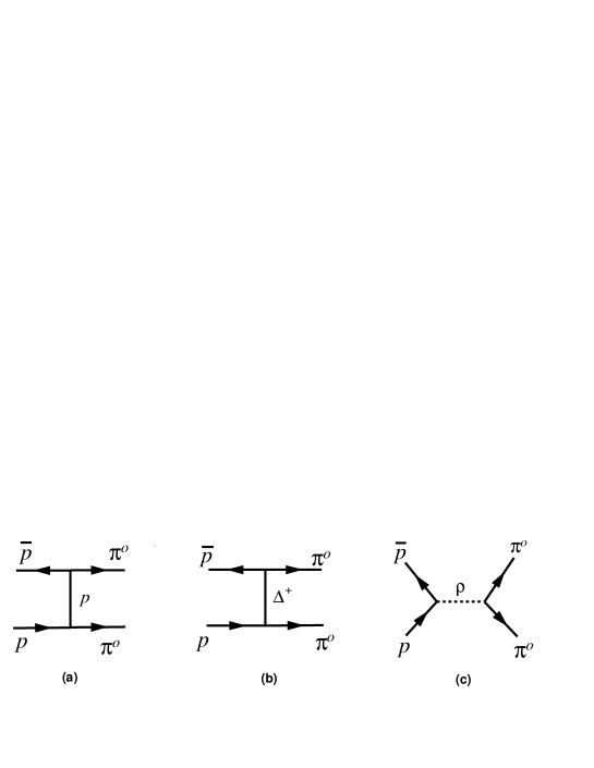
Figure 2: Feynman diagrams for different exchanged particles for the reaction $\bar{p}+p\to\pi^{0}+\pi^{0}$.

4 Comparison with existing data and Discussion

The following procedure was applied, in order to reproduce the collected data basis. The data, from Ref. [2] on neutral pion angular distributions, were first reproduced at best, with particular attention to the $s$ dependence of the cross section and the parameters were fixed. Besides the form factors listed above, we introduced 10% renormalization $N_{\rho}$ and a mild $s$-dependent relative phase $\phi_{\rho}=\phi_{0}+\phi_{1}s$ of the $\rho$ diagram, with $\phi_{0}=1$ and $\phi_{1}=0.004$. The necessary number of parameters is very limited and we checked that the results are quite stable towards a change of the parameters in a reasonable interval.

The existing data on neutral pion production from Ref. [2], together with the predictions of the model, are shown in Fig. 3 for energies spanning the range ($2.911\leq\sqrt{s}\leq 4.274$) GeV. The angular distributions are generally well reproduced at higher energies. The agreement is less satisfactory at low energies, where, in particular, an oscillation near $\cos\theta$=0 is no accounted in the present model. This could be possibly improved by adding other $s$-channel contributions. Moreover, the used form of Regge parametrization is not expected to work properly at low energies. Therefore the Regge factor was set to be unity for $s<s_{0}$.

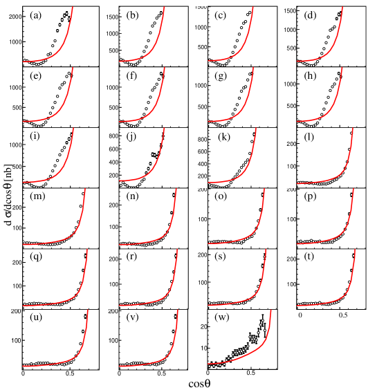
Figure 3: Angular distributions for the reaction $\bar{p}+p\to\pi^{0}+\pi^{0}$ for different values of $\sqrt{s}$: (a) $\sqrt{s}=2.911$ GeV, (b) $\sqrt{s}=2.950$ GeV, (c) $\sqrt{s}=2.975$ GeV, (d) $\sqrt{s}=2.979$ GeV, (e) $\sqrt{s}=2.981$ GeV, (f) $\sqrt{s}=2.985$ GeV, (g) $\sqrt{s}=2.990$ GeV, (h) $\sqrt{s}=2.994$ GeV, (i) $\sqrt{s}=3.005$ GeV, (j) $\sqrt{s}=3.050$ GeV, (k) $\sqrt{s}=3.095$ GeV, (l) $\sqrt{s}=3.524$ GeV, (m) $\sqrt{s}=3.526$ GeV, (n) $\sqrt{s}=3.556$ GeV, (o) $\sqrt{s}=3.591$ GeV, (p) $\sqrt{s}=3.595$ GeV, (q) $\sqrt{s}=3.613$ GeV, (r) $\sqrt{s}=3.616$ GeV, (s) $\sqrt{s}=3.619$ GeV, (t) $\sqrt{s}=3.621$ GeV, (u) $\sqrt{s}=3.686$ GeV, (w) $\sqrt{s}=4.274$ GeV. Data are taken from Ref. [2], the curve is the prediction of the present model.

The $s$ dependence of the model is shown in Fig. 4, and compared to the experimental data and to the $s^{-8}$ prediction from quark counting rules [25, 26] for $\cos\theta=0.0125$. The model follows reasonably well the predicted behavior for large angles and large energy. A change of slope for the lower energy data is expected and was already noticed in Ref. [2].

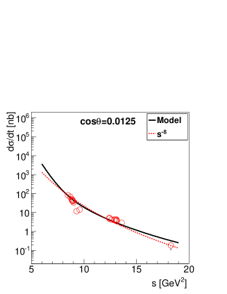
Figure 4: $s$-dependence for the reaction $\bar{p}+p\to\pi^{0}+\pi^{0}$ for the central region ($\cos\theta=0.0125$) and comparison of the model (black, solid line) with the $s^{-8}$ prediction from Ref. [25, 26] (red dashed line). Data are taken from Ref. [2].

Turning to charged pion production, one more diagram corresponding to $\Delta^{++}$ exchange has to be introduced in $u$ channel, to account for the asymmetric forward/backward production. The introduction of the $\Delta^{++}$ diagram allows to reproduce the backward angles for the charged pion data. As we use the same mass and couplings for the different charged states of the $\Delta$, the same form factors parameters for $\Delta^{+,0,++}$ are taken, not requiring any additional parameters.

The angular dependence for the reaction $\bar{p}+p\to\pi^{-}+\pi^{+}$, for different value of the total CMS energy $\sqrt{s}$ are shown in Fig. 5 (a-d).The agreement is satisfactory, taking into account that no rearrangement of the parameters was done. They correspond to very backward angles, and are also well reproduced by the model.

The results for the crossed channels $\pi^{\pm}$ elastic scattering are also reported in Fig. 5 (e-f), where data for the differential cross section span a small very forward or very backward angular region, bringing an additional test of the model.

The angular distribution for $\sqrt{s}$= 3.680 GeV is shown in Fig. 6 The total result (black, solid line) gives a good description of the data (red open circles) from Ref. [4] for charged pion production. All components and their interferences are illustrated. The main contribution at central angles is given by $\rho$ s-channel exchange, whereas $n$ exchange in $t$ channel dominates forward angles followed by $\Delta^{0}$ exchange. $\Delta^{++}$ represent the largest contribution for backward angles. The interferences are also shown. Their contribution affects the shape of the angular distribution, some of them being negative in part of the angular region.

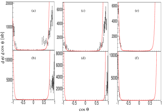
Figure 5: (color online) Angular dependence for the reaction $\bar{p}+p\to\pi^{-}+\pi^{+}$, for different value of the total CMS energy $\sqrt{s}$ : (a) $\sqrt{s}=3.362$ GeV from Ref. [5], (b) $\sqrt{s}=3.627$ GeV from Ref. [27], (c) $\sqrt{s}=3.680$ GeV from Ref. [4], (d) $\sqrt{s}=4.559$ GeV from Ref. [28]. The corresponding data from the elastic reactions $\pi+p\to\pi+p$ are also reported: (e) $\sqrt{s}=3.463$ GeV from Ref. [29], (f) $\sqrt{s}=3.747$ GeV from Ref. [30].

5 Conclusions

An model, built on effective meson Lagrangian, has been build in order to reproduce the existing data for two pion production in proton-antiproton annihilation at moderate and large energies. Form factors and Regge factors are implemented and parameters adjusted to the existing data for neutral and charged pion pair production. Coupling constants are fixed from the known properties of the corresponding decay channels. The agreement with a large set of data is satisfactory for the angular dependence as well as the energy dependence of the cross section. At large angles the model follows naturally the expected behavior from quark counting rules.

A comparison with data from elastic $\pi^{\pm}p\to\pi^{\pm}p$, using crossing symmetry prescriptions shows a good agreement also at very forward and backward angles, within the uncertainty. Discussion about validity of crossing symmetry can be found in Refs. [5, 29, 27]. The present results verify that crossing symmetry works at least at backward angles, where one diagram is dominant.

This model can be extended to other binary channels, with appropriate changes of constants. The implementation to MonteCarlo simulations for predictions and optimization to coming experiments is also foreseen.

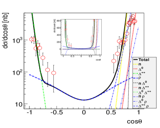
Figure 6: (color online) $\cos\theta$-dependence for the reaction $\bar{p}+p\to\pi^{-}+\pi^{+}$ for $\sqrt{s}$= 3.680 GeV (black, solid line) where the different components are illustrated: $n$ exchange (yellow thick short dash line) dominates at forward angle, followed by $\Delta_{0}$( read thick dotted line) $\Delta^{++}$ (green thick dash-dotted line) represent the largest contribution for backward angles, $\rho$ channel (blue thick long dash line) dominates at large angles, The interferences are $n\Delta^{0}$ (thin black short-dash line) , $n\Delta^{++}$ (thin red dotted line), $\Delta^{0}\Delta^{++}$(green thin short dash-dotted line), $n\rho$(blue thin long-dashed dotted line) , $\Delta^{0}\rho$ (blue thin dash-dotted line), $\Delta^{++}\rho$ (blue thin long dash line). visible at large angles. Data are taken from Ref. [4]

.

6 Acknowledgments

Thanks are due to D. Marchand and A. Dorokhov, for useful discussions and interest in this work. One of us (Yu.B) acknowledges kind hospitality at IPN Orsay, in frame of JINR-IN2P3 agreement.

7 Appendix

The relevant formulas for the amplitudes and their interferences are given below.

7.1 Neutron exchange

The amplitude for nucleon exchange is written as:

$${\cal M}_{N}=\displaystyle\frac{g^{2}_{\pi NN}}{q_{t}^{2}-M_{N}^{2}}\bar{v}(p_{1})(-\hat{q}_{t}+M_{N})u(p_{2}).$$ (11)

where $u(p_{2})(\bar{v}(p_{1}))$, are the four-component spinors of the proton(antiproton), which obey the Dirac equation. The matrix element squared for the diagram corresponding to neutron exchange, Fig. 1a is written as:

$$|\overline{{\cal M}_{N}}|^{2} = \displaystyle\frac{g^{4}_{\pi NN}}{(q_{t}^{2}-M_{N})}Tr\left[(\hat{p}_{1}-M_{N})(-\hat{q}_{t}+M_{N})(\hat{p}_{2}+M_{N})(-\hat{q}_{t}+M_{N})\right]$$ (12)

$$= -2\displaystyle\frac{g^{4}_{\pi NN}}{(t-M_{N})^{2}}\left[m^{4}+(M_{N}^{2}-t)(M_{N}^{2}-s-t+2m_{\pi})\right],$$

with $q_{t}=k_{1}-p_{1}=p_{2}-k_{2}$, $q_{t}^{2}=t$.

7.2 $t$-Exchange of $\Delta^{0}$

The specific ingredients for $\Delta$ exchange, Fig. 1b, are related to the spin 3/2 nature of the $\Delta$-resonance . For the $\Delta$-spin-vector, $U_{\Delta}$, we take the expression from [31]: where the density matrix is

$$P_{\mu\nu}=U_{\mu}^{\Delta}(p_{\Delta})\bar{U}_{\nu}^{*\Delta}(p_{\Delta})=-g_{\mu\nu}+\frac{1}{3}\gamma_{\mu}\gamma_{\nu}+\frac{\gamma_{\mu}P_{\nu}-\gamma_{\nu}P_{\mu}}{3M_{\Delta}}+\frac{2}{3}\frac{P_{\mu}P_{\nu}}{M_{\Delta}^{2}}.$$ (13)

and:

$$a)\displaystyle\frac{i}{(2\pi)^{4}}\displaystyle\frac{\hat{q}_{t}+M_{\Delta}}{q_{t}^{2}-M_{\Delta}^{2}}P_{\mu\nu},~{}~{}b)-i(2\pi)^{4}g_{\Delta\pi N}k_{1}^{\mu}$$ (14)

are the expressions for a) the $\Delta$ propagator and b) the vertex $\Delta\to\pi N$. $M_{\Delta}=1.232\pm 2$ MeV is the weighted mass of the $\Delta$ resonance, (i.e., the mass averaged over $\Delta$-multiplet), and $g_{\Delta\pi N}$ is the coupling constant for the vertex $\Delta\to\pi N$.

The matrix element for the diagram Fig. 1.b is:

$${\cal M}_{\Delta^{0}}=-\displaystyle\frac{g^{2}_{\Delta\pi N}}{t-M_{\Delta}^{2}}\bar{v}(p_{1})(\hat{q}_{t}+M_{\Delta})P_{\mu\nu}(q_{t})u(p_{2})k_{1}^{\mu}k_{2}^{\nu}.$$ (15)

Squaring the amplitude one has

$$|\overline{{\cal M}_{\Delta^{0}}}|^{2}=\displaystyle\frac{g^{4}_{\Delta\pi N}}{(t-M_{\Delta}^{2})^{2}}k_{1}^{\mu}k_{2}^{\nu}k_{1}^{\alpha}k_{2}^{\beta}Tr\left[(\hat{p}_{1}-M_{N})(\hat{q}_{t}+M_{\Delta})P_{\mu\nu}(q_{t})(\hat{p}_{2}+M_{N})\tilde{P}_{\alpha\beta}(q_{t})(\hat{q}_{t}+M_{\Delta})\right].$$ (16)

In order to find the value of $g_{\Delta N\pi}$ coupling constant we consider the decay width of $\Delta$ into nucleon and pion:

$$\Gamma_{\Delta}=\displaystyle\frac{3}{2}\displaystyle\frac{|\vec{p}|}{32\pi M_{\Delta}^{2}}|{\cal M}(\Delta\to N\pi)|^{2},$$ (17)

and using the experimental values of the decay width $\Gamma_{\Delta}=117\pm 3$ MeV [21], one can estimate $g_{\Delta N\pi}=15.7\pm 0.4$ GeV^-1.

7.3 $u$-exchange of $\Delta^{++}$

The diagram in Fig. 1c corresponds to $\pi^{-}$ emitted at backward angle involves the exchange of $\Delta^{++}$ and can be obtained from $t$-exchange 1b with the replacements: $t\leftrightarrow u$ and $k_{1}\leftrightarrow k_{2}$.

7.4 Interferences with $\Delta$

7.4.1 The $\Delta^{0}-N$ interference

$$2Re[M_{N}^{*}M_{\Delta}^{0}]=2Re\Bigg{\{}\displaystyle\frac{g^{2}_{\pi NN}g^{2}_{\Delta\pi N}}{(t-M_{N}^{2})(t-M_{\Delta}^{2})}Tr\left[(\hat{p}_{1}+M_{N})(-\hat{q}_{t}+M_{N})(\hat{p}_{2}+M_{N})\tilde{P}_{\mu\nu}(q_{t})(\hat{q}_{u}+M_{\Delta})\right]k_{1}^{\mu}k_{2}^{\nu}\Bigg{\}},$$ (18)

with $q_{u}=k_{2}-p_{1}=p_{2}-k_{1}$, $q_{u}^{2}=u$.

7.4.2 The $\Delta^{++}-N$ interference

$$2Re[M_{N}^{*}M_{\Delta}^{++}]=2Re\Bigg{\{}\displaystyle\frac{g^{2}_{\pi NN}g^{2}_{\Delta\pi N}}{(u-M_{\Delta}^{2})(t-M_{N}^{2})}Tr\left[(\hat{p}_{1}+M_{N})(-\hat{q}_{t}+M_{N})(\hat{p}_{2}+M_{N})\tilde{P}_{\mu\nu}(q_{u})(\hat{q}_{u}+M_{\Delta})\right]k_{1}^{\nu}k_{2}^{\mu}\Bigg{\}}.$$ (19)

7.4.3 The $\Delta^{++}-\Delta^{0}$ interference

$$2Re[M_{\Delta}^{*0}M_{\Delta}^{++}]=2Re\Bigg{\{}\displaystyle\frac{g^{4}_{\Delta\pi N}}{(t-M_{\Delta}^{2})(u-M_{\Delta}^{2})}Tr\left[(\hat{p}_{1}-M_{N})(\hat{q}_{t}+M_{N})P_{\mu\nu}(q_{t})(\hat{p}_{2}+M_{N})\tilde{P}_{\alpha\beta}(q_{u})(\hat{q}_{u}+M_{\Delta})\right]k_{1}^{\mu}k_{2}^{\nu}k_{2}^{\alpha}k_{1}^{\beta}\Bigg{\}}.$$ (20)

7.5 $s$-exchange of $\rho$ meson

The largest contribution to meson exchange in s-channel, Fig 1d, is given by the $\rho$-meson, with $\sim 100\%$ branching ratio into two pions. For the a) $\rho$- propagator and b) the $\rho\pi\pi$ vertex we take

$$a)-\displaystyle\frac{i}{(2\pi)^{4}}\left[\displaystyle\frac{g_{\mu\nu}-(q_{s}^{\mu}q_{s}^{\nu})/{m_{\rho}^{2}}}{q_{s}^{2}-m_{\rho}^{2}+i\sqrt{q_{s}^{2}}\Gamma_{\rho}(q_{s}^{2})}\right],~{}~{}b)-ig_{\rho\pi\pi}(k_{1}-k_{2})^{\nu}(2\pi)^{4},~{}q_{s}=p_{1}+p_{2}=k_{1}+k_{2},$$ (21)

where $g_{\mu\nu}$ is the symmetric tensor, and $q_{s}^{2}=s$. The matrix element is written as:

$${\cal M}_{\rho}=\displaystyle\frac{g_{\rho pp}g_{\rho\pi\pi}}{[s-m_{\rho}^{2}+i\sqrt{s}\Gamma_{\rho}(s)]}[\bar{v}(p_{1})\Gamma^{\mu}(q)u(p_{2})](k_{1}-k_{2})^{\nu}\left\{g_{\mu\nu}-\displaystyle\frac{q_{\mu}q_{\nu}}{m_{\rho}^{2}}\right\},$$ (22)

Squaring the amplitude one gets:

$$|\overline{{\cal M}_{\rho}}|^{2} = \displaystyle\frac{g^{2}_{\rho NN}g^{2}_{\rho\pi\pi}}{[s-m_{\rho}^{2}+i\sqrt{s}\Gamma_{\rho}(s)]^{2}}(k_{1}-k_{2})^{\nu}(k_{1}-k_{2})^{\beta}\left(g_{\mu\nu}-\displaystyle\frac{(q_{s})_{\mu}(q_{s})_{\nu}}{m_{\rho}^{2}}\right)\left(g_{\alpha\beta}-\displaystyle\frac{(q_{s})_{\alpha}(q_{s})_{\beta}}{m_{\rho}^{2}}\right)$$ (23)

$$Tr\left[(\hat{p}_{1}-M_{N})\Gamma^{\mu}(q_{s})(\hat{p}_{2}+M_{N})\Gamma^{\alpha}(q_{s})\right].$$

The coupling constant $g_{\rho\to\pi\pi}$ is found from the the experimental value of the total width $\Gamma$ for the decay $\rho\to\pi\pi$: $\Gamma(\rho)$ = 149.1 $\pm$ 0.8 MeV [21]. The branching ratio into two pions is $\approx 100\%$. The total width has the form:

$$\Gamma=\displaystyle\frac{4}{3}\frac{g_{\rho\pi\pi}^{2}}{16\pi m_{\rho}^{2}}(m_{\rho}^{2}-4m_{\pi}^{2})^{3/2},$$ (24)

where we added a factor 4/3 to take into account that there are three possible initial states of the $\rho$ meson and four possible charged decays. Inverting Eq. (24), using the experimental value for the decay width one can get the following value of the coupling constant: $g_{\rho\pi\pi}=5.175\pm 0.017$.

7.6 Interferences with $\rho$

7.6.1 The $N-\rho$ interference

$$2Re[M_{N}^{*}M_{\rho}] = 2Re\left\{\displaystyle\frac{g_{\pi NN}g_{\rho\pi\pi}g^{2}_{\rho NN}}{[s-m_{\rho}^{2}+i\sqrt{s}\Gamma_{\rho}(s)](t-M_{N}^{2})}Tr\left[(\hat{p}_{1}-M_{N})\Gamma^{\mu}(q_{s})(\hat{p}_{2}+M_{N})\tilde{P}_{\alpha\beta}(q_{t})(-\hat{q}_{t}+M_{N})\right]\right.$$ (25)

$$\left.k_{1}^{\alpha}k_{2}^{\beta}(k_{1}-k_{2})^{\nu}\left(g_{\mu\nu}-\displaystyle\frac{q_{\mu}q_{\nu}}{m_{\rho}^{2}}\right)\right\}.$$

7.6.2 The $\Delta^{0}-\rho$ interference

$$2Re[M_{\Delta^{0}}m_{\rho}^{*}] = 2Re\left\{\displaystyle\frac{g_{\rho NN}g_{\rho\pi\pi}g^{2}_{\Delta\rho N}}{[s-m_{\rho}^{2}+i\sqrt{s}\Gamma_{\rho}(s)](t-M_{\Delta}^{2})}Tr\left[(\hat{p}_{1}-M_{N})\Gamma^{\mu}(q_{s})(\hat{p}_{2}+M_{N})\tilde{P}_{\alpha\beta}(q_{t})(-\hat{q}_{t}+M_{\Delta})\right]\right.$$ (26)

$$\left.k_{1}^{\alpha}k_{2}^{\beta}(k_{1}-k_{2})^{\nu}\left(g_{\mu\nu}-\displaystyle\frac{q_{\mu}q_{\nu}}{m_{\rho}^{2}}\right)\right\}.$$

7.6.3 The $\Delta^{++}-\rho$ interference

$$2Re[M_{\Delta^{++}}m_{\rho}^{*}] = 2Re\left\{\displaystyle\frac{g_{\rho NN}g_{\rho\pi\pi}g^{2}_{\Delta\rho N}}{[s-m_{\rho}^{2}+i\sqrt{s}\Gamma_{\rho}(s)](u-M_{\Delta}^{2})}Tr\left[(\hat{p}_{1}-M_{N})\Gamma^{\mu}(q_{s})(\hat{p}_{2}+M_{N})\tilde{P}_{\alpha\beta}(q_{u})(-\hat{q}_{u}+M_{\Delta})\right]\right.$$ (27)

$$\left.k_{1}^{\alpha}k_{2}^{\beta}(k_{1}-k_{2})^{\nu}\left(g_{\mu\nu}-\displaystyle\frac{q_{\mu}q_{\nu}}{m_{\rho}^{2}}\right)\right\}.$$

References

- [1] C. B. Dover, T. Gutsche, M. Maruyama, A. Faessler, The Physics of nucleon - anti-nucleon annihilation, Prog. Part. Nucl. Phys. 29 (1992) 87–174. doi:10.1016/0146-6410(92)90004-L.
- [2] T. Armstrong, et al., Two-body neutral final states produced in annihilations at 2.911-GeV 3.686-GeV, Phys.Rev. D56 (1997) 2509–2531. doi:10.1103/PhysRevD.56.2509.
- [3] E. Eisenhandler, W. Gibson, C. Hojvat, P. Kalmus, L. L. C. Kwong, et al., Measurement of Differential Cross-Sections for anti-Proton-Proton Annihilation Into Charged Pion and Kaon Pairs Between 0.79-GeV/c and 2.43-GeV/c, Nucl.Phys. B96 (1975) 109. doi:10.1016/0550-3213(75)90461-7.
- [4] T. Buran, A. Eide, P. Helgaker, P. Lehmann, A. Lundby, et al., Anti-Proton-Proton Annihilation Into pi+ pi- and K+ K- at 6.2-GeV/c, Nucl.Phys. B116 (1976) 51. doi:10.1016/0550-3213(76)90311-4.
- [5] A. Eide, P. Lehmann, A. Lundby, C. Baglin, P. Briandet, et al., Elastic scattering and two-body annihilations at 5 GeV/c, Nucl.Phys. B60 (1973) 173–220. doi:10.1016/0550-3213(73)90176-4.
- [6] B. Moussallam, ANTI-P P —¿ PI PI IN A BARYON EXCHANGE POTENTIAL MODEL, Nucl. Phys. A429 (1984) 429–444. doi:10.1016/0375-9474(84)90690-0.
- [7] J. Van de Wiele, S. Ong, Regge description of two pseudoscalar meson production in antiproton-proton annihilation, Eur.Phys.J. A46 (2010) 291–298. arXiv:1004.2152, doi:10.1140/epja/i2010-11044-7.
- [8] A. ”Dbeyssi, ”study of the internal structure of the proton with the panda experiment at fair”, Ph.D. thesis, Université Paris-sud (2013).
- [9] G. Bardin, G. Burgun, R. Calabrese, G. Capon, R. Carlin, et al., A Measurement of the Reaction for 158-MeV/ 275-MeV/, Phys.Lett. B192 (1987) 471. doi:10.1016/0370-2693(87)90140-7.
- [10] G. Bardin, G. Burgun, R. Calabrese, G. Capon, R. Carlin, et al., Determination of the electric and magnetic form-factors of the proton in the timelike region, Nucl.Phys. B411 (1994) 3–32. doi:10.1016/0550-3213(94)90052-3.
- [11] T. Tanimori, T. Fujii, T. Kageyama, K. Nakamura, F. Sai, et al., Obrevation of an enhancement in , cross sections at momentum of approximately 500-MeV/c, Phys.Rev.Lett. 55 (1985) 1835–1838. doi:10.1103/PhysRevLett.55.1835.
- [12] F. Sai, S. Sakamoto, S. Yamamoto, Measurement of Annihilation Cross-sections Into Charged Particles in the Momentum Range 374-MeV/ - 680-MeV/, Nucl.Phys. B213 (1983) 371. doi:10.1016/0550-3213(83)90227-4.
- [13] D. Ward, A. Simmons, R. Ansorge, C. Booth, J. Carter, et al., Exclusive annihilation processes in 8.8-GeV interactions and comparisons between nonannihilations and interactions , Nucl.Phys. B172 (1980) 302. doi:10.1016/0550-3213(80)90169-8.
- [14] C. Chen, T. Fields, D. Rhines, J. Whitmore, anti-p p Interactions at 2.32-GeV/c, Phys.Rev. D17 (1978) 42. doi:10.1103/PhysRevD.17.42.
- [15] G. Bassompierre, et al., First Determination of the Proton Electromagnetic Form-Factors at the Threshold of the Timelike Region, Phys.Lett. B68 (1977) 477. doi:10.1016/0370-2693(77)90475-0.
- [16] P. Eastman, M. Ming, B. Oh, D. Parker, G. Smith, et al., A formation study of n anti-n interactions between 1.51 and 2.90 gev/c. i. topological and reaction cross-sections, Nucl.Phys. B51 (1973) 29–56. doi:10.1016/0550-3213(73)90499-9.
- [17] M. Mandelkern, R. Burns, P. Condon, J. Schultz, Proton-antiproton annihilation into and k+ k- from 700 to 1100 mev/c, Phys.Rev. D4 (1971) 2658–2666. doi:10.1103/PhysRevD.4.2658.
-
[18]
V. Domingo, G. Fisher, L. M. Libby, R. Sears,
Two
meson final states in interactions of 2.7 gev/c p, Physics Letters
B 25 (7) (1967) 486 – 488.
doi:http://dx.doi.org/10.1016/0370-2693(67)90118-9.
URL http://www.sciencedirect.com/science/article/pii/0370269367901189 - [19] T. Armstrong, et al., Backward scattering in , , and at 8-GeV/c and 12-GeV/c, Nucl.Phys. B284 (1987) 643. doi:10.1016/0550-3213(87)90054-X.
-
[20]
R. Machleidt,
High-precision,
charge-dependent bonn nucleon-nucleon potential, Phys. Rev. C 63 (2001)
024001.
doi:10.1103/PhysRevC.63.024001.
URL http://link.aps.org/doi/10.1103/PhysRevC.63.024001 - [21] K. Olive, et al., Review of Particle Physics, Chin.Phys. C38 (2014) 090001. doi:10.1088/1674-1137/38/9/090001.
- [22] A. B. Kaidalov, Regge poles in QCDarXiv:hep-ph/0103011.
- [23] E. Kuraev, Y. Bystritskiy, V. Bytev, E. Tomasi-Gustafsson, Annihilation of and through -meson intermediate statearXiv:1012.5720.
- [24] C. Fernandez-Ramirez, E. Moya de Guerra, J. M. Udias, Effective Lagrangian approach to pion photoproduction from the nucleon, Annals Phys. 321 (2006) 1408–1456. arXiv:nucl-th/0509020, doi:10.1016/j.aop.2006.02.009.
- [25] V. Matveev, R. Muradyan, A. Tavkhelidze, Automodelity in strong interactions, Teor.Mat.Fiz. 15 (1973) 332–339.
- [26] S. J. Brodsky, G. R. Farrar, Scaling Laws at Large Transverse Momentum, Phys.Rev.Lett. 31 (1973) 1153–1156. doi:10.1103/PhysRevLett.31.1153.
- [27] N. Stein, R. Edelstein, D. Green, H. Halpern, E. Makuchowski, et al., Comparison of the Line Reversed Channels and at 6-GeV/c, Phys.Rev.Lett. 39 (1977) 378–381. doi:10.1103/PhysRevLett.39.378.
- [28] A. Berglund, T. Buran, P. Carlson, C. Damerell, I. Endo, et al., A Study of the Reaction at 10-GeV/c, Nucl.Phys. B137 (1978) 276–282. doi:10.1016/0550-3213(78)90521-7.
-
[29]
D. P. Owen, F. C. Peterson, J. Orear, A. L. Read, D. G. Ryan, D. H. White,
A. Ashmore, C. J. S. Damerell, W. R. Frisken, R. Rubinstein,
High-energy elastic
scattering of , , and on hydrogen at c.m.
angles from 22∘ to 180∘, Phys. Rev. 181 (1969) 1794–1807.
doi:10.1103/PhysRev.181.1794.
URL http://link.aps.org/doi/10.1103/PhysRev.181.1794 -
[30]
W. Baker, K. Berkelman, P. Carlson, G. Fisher, P. Fleury, D. Hartill,
R. Kalbach, A. Lundby, S. Mukhin, R. Nierhaus, K. Pretzl, J. Woulds,
Elastic
forward and backward scattering of π− and k-mesons at 5.2 and 7.0 gev/c,
Nuclear Physics B 25 (2) (1971) 385 – 410.
doi:http://dx.doi.org/10.1016/0550-3213(71)90408-1.
URL http://www.sciencedirect.com/science/article/pii/0550321371904081 - [31] A. Akhiezer, M. Rekalo, Hadron Electrodynamics, Naukova Dumka, Kiev, 1977.