Thermalization in a 1D Rydberg gas:
validity of the microcanonical ensemble hypothesis

Abstract

We question the microcanonical hypothesis, often made to account for the thermalization of complex closed quantum systems, on the specific example of a chain of two-level atoms optically driven by a resonant laser beam and strongly interacting via Rydberg-Rydberg dipole-dipole interactions. Along its (necessarily unitary) evolution, this system is indeed expected to thermalize, i.e. observables, such as the number of excitations, stop oscillating and reach equilibrium-like expectation values. The latter are often calculated through assuming the system can be effectively described by a thermal-like microcanonical state. Here, we compare the distribution of excitations in the chain calculated either according to the microcanonical assumption or through direct exact numerical simulation. This allows us to show the limitations of the thermal equilibrium hypothesis and precise its applicability conditions.

I Introduction

Due to their large dipole moments G94 , Rydberg atoms experience strong long-range dipole-dipole interactions. Within the last decade, this feature has been put forward as the key ingredient of different promising atomic quantum-processing scenarios SWM10 . For instance, Rydberg-Rydberg interactions can be used to perform two-qubit logic operations in individual-atom systems by shifting a transition off-resonance in an atom, depending on the internal state of another atom in its immediate neighborhood JCZ00 ; PRS02 ; SW05 . In a mesoscopic ensemble, dipole-dipole interactions are able to inhibit transitions into collective states that contain more than one Rydberg excitation, thus leading to the so-called Rydberg blockade. First predicted in LFC01 , this phenomenon was locally observed in laser-cooled atomic systems TFS04 ; SRA04 ; CRB05 ; AVG98 ; VVZ06 and could in principle be used in the future to manipulate and entangle collective excitation states of mesoscopic ensembles of cold atoms which could therefore be run as quantum processors LFC01 ; BMM07 ; BMS07 ; BPS08 or repeaters ZMH10 ; HHH10 ; BCA12 . Rydberg atomic ensembles are also investigated on quantum non-linear optical purposes WA13 : converting photons into so-called Rydberg polaritons which strongly interact through dipole-dipole interaction, it seems indeed possible to generate giant non-linearities in the quantum regime, i.e. to effectively implement photon-photon interactions PFL12 ; PBS12 ; MSP13 .

The exact calculation of the time-dependent state of an ensemble of atoms resonantly laser-driven towards a Rydberg level constitutes a highly non-trivial coupled many-body problem. Such a complex system, however, often shows an effective thermalization behavior LOG10 ; AL12 ; BMFALA13 : observables, such as the number of Rydberg excitations, indeed tend to quasistationary values which can be computed assuming the system is in a thermal equilibrium state, either in the canonical LOG10 or microcanonical AL12 ; BMFALA13 ensembles. Considering the same system as in AL12 ; BMFALA13 , we compare the predictions of the microcanonical ensemble assumption to a numerical simulation of the unitary evolution of a $100$-particle system, confirmed by a simplified analytical treatment. The discrepancies we observe allow us to show the limitations of the equilibrium hypothesis and to precise its applicability conditions.

The paper is organized as follows. In Sec. II, we present the physical system and simplified model. In Sec. III, we give an analytical description of the distribution of excitations according to the microcanonical ensemble. In Sec. IV, we numerically compute the distribution of excitations and apply a simplified analytical treatment which allows us to satisfactorily reproduce the results of the full simulation, in the regime of at most 2 excitations. In Sec. V, we discuss and compare the results obtained according to the different approaches, before concluding in Sec. VI.

II Model and approximations

We consider a system of $N$ identical atoms located along a line of length $L$. The Hilbert space of each atom is assumed to be restricted to the ground state $\left|g\right\rangle$ and a highly excited (so-called) Rydberg state $\left|r\right\rangle$. In the ensemble “vacuum state” $\left|\varnothing\right\rangle$, all atoms are in the ground state: $\left|\varnothing\right\rangle\equiv\left|g\dots g\right\rangle$. Denoting by $\sigma_{+}\equiv\left|e\right\rangle\left\langle g\right|$ and $\sigma_{-}\equiv\sigma_{+}^{\dagger}$ the usual raising and lowering operators for a two-level atom, one defines the ensemble state $\left|i\right\rangle\equiv\sigma_{+}^{i}\left|\varnothing\right\rangle=\left|g_{1},\dots,g_{i-1},r_{i},g_{i+1},\dots,g_{N}\right\rangle$ in which the $i^{\text{th}}$ atom is Rydberg-excited while the others are in the ground state. In the same way, one can define the doubly excited state $\left|i,j\right\rangle\equiv\sigma_{+}^{\left(i\right)}\sigma_{+}^{\left(j\right)}\left|\varnothing\right\rangle$ which contains only two Rydberg excitations at positions $i$ and $j$, and more generally any arbitrary multiply excited state $\left|i,j,k,\dots\right\rangle\equiv\sigma_{+}^{\left(i\right)}\sigma_{+}^{\left(j\right)}\sigma_{+}^{\left(k\right)}\dots\left|\varnothing\right\rangle$.

The atomic ensemble is subject to a laser beam which resonantly drives the transition $\left|g\right\rangle\leftrightarrow\left|r\right\rangle$: in the rotating wave approximation, this process is simply described by the Hamiltonian $H_{L}=\hbar\Omega\sum_{k=1}^{n}\left(\sigma_{+}^{k}+\sigma_{-}^{k}\right)$, where $\Omega$ denotes the laser Rabi frequency. Moreover, when lying in their Rydberg state, two atoms interact through the (strong) dipole-dipole interaction (this interaction is negligible when at least one atom in the pair is in the ground state): the corresponding Hamiltonian is

$$V_{dd}=\hbar C_{6}\sum_{k\neq m}\frac{n_{m}n_{k}}{d(m,k)^{6}}$$ (1)

where $C_{6}$ is the van der Waals interaction coefficient, $n_{k}\equiv\sigma_{+}^{k}\sigma_{-}^{k}$ the projector onto the Rydberg state for the $k^{\text{th}}$ atom and $d(m,k)$ is the distance between the $m^{\text{th}}$ and the $k^{\text{th}}$ atoms. Finally, the full Hamiltonian governing the dynamics of the system is

$$H =H_{L}+V_{dd}$$ (2)

Starting in the ensemble vacuum state $\left|\varnothing\right\rangle$, in the absence of interatomic interactions, each atom in the sample would independently undergo Rabi oscillations. Because of dipole-dipole interactions, atoms actually get entangled during their evolution, according to the so-called Rydberg blockade phenomenon LFC01 . To understand this mechanism, let us first consider the simple case of two atoms. If they are “close enough” so that their dipole-dipole interaction overwhelms the laser Rabi frequency, their simultaneous excitation into the Rydberg state becomes impossible since the doubly excited state is strongly shifted out of resonance. As a rule of thumb, one can define the typical distance $R_{b}$, called the blockade radius, at which the blockade starts being effective as the distance for which the van der Waals interaction becomes comparable with the laser excitation, i.e $R_{b}\approx\left(\frac{C_{6}}{\Omega}\right)^{\frac{1}{6}}$. Now turning to the full sample, it is clear that dipole-dipole interactions forbid the system to explore its full Hilbert space: too off-resonant configurations, i.e. ensemble states in which two Rydberg excited atoms are closer than the radius $R_{b}$, will indeed never be substantially populated. In other words, due to the Rydberg blockade the system is bound to essentially evolve in the subspace of “allowed states” in which excited atoms are separated at least by $R_{b}$ (Note that in a 3D geometric arrangement, each Rydberg excited atom creates an “exclusion” sphere of radius $R_{b}$ often called a “Rydberg bubble”).

Though simple in its form, the Hamiltonian Eq. (2) leads to complex many-body dynamics. In particular, besides the Rydberg blockade phenomenon qualitatively described above, it was shown to yield thermalization effects LOG10 . The full computation of the dynamics is intractable for large numbers of atoms and one must resort to approximations. Following LOG10 , we shall make the hardcore Rydberg sphere assumption, that is we shall merely discard all atomic configurations in which two Rydberg excitations are closer than $R_{b}$, while keeping the others; moreover, we shall make the simplistic approximation that in the allowed subspace the dipole-dipole Hamiltonian is zero. In this approximation the full Hamiltonian therefore becomes

$$H\approx\hbar\Omega\sum_{k=1}^{n}(\tilde{\sigma}_{+}^{k}+\tilde{\sigma}_{-}^{k})$$ (3)

where $\tilde{\sigma}_{+}^{k}$ is the raising operator of the $k^{\text{th}}$ atom restricted to the allowed configuration subspace, i.e. the operator which excites the $k^{\text{th}}$ atom into the Rydberg state provided that no other Rydberg atom is in the range $R_{b}$.

III Thermalized state: Analytical results from the microcanonical ensemble assumption

Analytical AGL12 ; JAG13 and numerical LOG10 investigations of the approximate Hamiltonian Eq. (3) both predict thermalization to occur in the system. Intuitively, this phenomenon results from the destructive interferences between different frequency components of the evolved vector state: for large times, due to the complexity of the Hilbert space and the high connectivity of the basis states, observables, such as the number of Rydberg-excited atoms, are expected to stop oscillating and tend to quasistationary values. According to the microcanonical ensemble assumption AL12 ; BMFALA13 , these values can be accounted for by assuming an effective thermal equilibrium-like state for the system which consists of an equiprobable statistical mixture of all allowed states.

The common probability of all the components in this mixture is therefore simply given by the inverse of the total number $\mathcal{N}$ of allowed states. This number can be determined by summing all numbers $\mathcal{N}(\nu)$ of allowed configurations with exactly $\nu$ excitations, which, as we show below, can be calculated through a straightforward combinatorial argument. From $\mathcal{N}(\nu)$, one easily computes the average number of excitations $\left\langle\nu\right\rangle$ and, in the limit of a continuous distribution, one can even deduce a simple expression of the spatial density of Rydberg excitations.

In this section, we present our analytical calculations in detail and compare our results to numerical Monte Carlo simulations presented in BMFALA13 .

III.1 Number of allowed states and average excitation number: combinatorial analysis

The goal of this subsection is to compute the average number of Rydberg excitations observed in the thermalized state according to the microcanonical ensemble assumption. For sake of simplicity, we assume that the atoms are located at the nodes of a regular 1D lattice of step $a$. The distance between the $i^{\text{th}}$ and $j^{\text{th}}$ atoms is therefore $d(i,j)=a\left|i-j\right|$ while the total length of the line is given by $L=\left(N-1\right)a$. The quantity $n_{b}\equiv\left\lfloor\frac{R_{b}}{a}\right\rfloor$, where $\left\lfloor\cdot\right\rfloor$ denotes the lower integer part, represents the minimal number of ground-state atoms which must lie between two Rydberg excitations in an allowed atomic configuration according to the hardcore Rydberg sphere assumption. Finally, we introduce the real parameter $\Lambda\equiv\frac{L}{R_{b}}$. Adding one to its integer part gives the maximum number of Rydberg excitations the sample can accommodate for: $\nu_{\max}=\left\lfloor\Lambda\right\rfloor+1$.

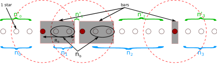
$\overbrace{\bigstar\bigstar\bigstar}^{n^{\prime}_{0}}|\overbrace{\phantom{|}}^{n^{\prime}_{1}}|\overbrace{\bigstar\bigstar\bigstar\bigstar}^{n^{\prime}_{2}}|\overbrace{\bigstar\bigstar\bigstar}^{n^{\prime}_{3}}$

Figure 1: : Description of a configuration of the excitations and mapping to the “Stars and bars” problem. An excited atom with all the atoms on its right closer than $R_{b}$ correspond to a bar, except for the last bar constituted only by the last excited atom. Each remaining atom represent a star. The depicted configuration corresponds to $L=16$, $N=17$, $2a\leq R_{b}<3a$, $n_{b}=2$, $\{n_{k}\}_{k}=\{3,2,6,3\}$, $\{n^{\prime}_{k}\}_{k}=\{3,0,4,3\}$.

To begin with, we compute the number of allowed states which comprise a given number of excitations $\nu$. In such a state, the $\nu$ Rydberg excitations split the sample into $\left(\nu+1\right)$ groups of $n_{k=0,\dots,\nu}$ ground-state atoms (see Fig. 1), with the convention that the zeroth and $\nu^{\text{th}}$ groups are on the left and the right of the leftmost and rightmost excited atoms, respectively, and allowing $n_{0}$ and $n_{\nu}$ to be zero. The state indeed corresponds to an allowed configuration if it satisfies the hardcore Rydberg sphere condition, i.e. $n_{k}\geq n_{b}$ for $1\leq k\leq\left(\nu-1\right)$, under the prescription $\sum_{k=0}^{\nu}n_{k}=N-\nu$: finding the number of allowed states with $\nu$ excitations is therefore equivalent to computing the number of sets of integers $\left\{n_{k=0,\dots,\nu}\right\}$ which satisfy the two previous conditions. A slight modification in the formulation of this problem turns it into a standard combinatorial calculation as we shall now show. We first note that an allowed atomic configuration can be uniquely determined by the alternative set of numbers $\left\{n{}_{k}^{\prime}\right\}$ defined by

$$n_{0}^{\prime} \equiv n_{0}$$

$$n_{k}^{\prime} \equiv n_{k}-n_{b}\;\text{for }1\leq k\leq\nu-1$$

$$n_{\nu}^{\prime} \equiv n_{\nu}$$

which satisfy the conditions $n_{k}^{\prime}\geq 0$ and $\sum_{k=0}^{\nu}n^{\prime}_{k}=N-1-(\nu-1)(n_{b}+1)$. This change of variables suggests to associate the original atomic arrangement with an abstract linear distribution of $\left[N-1-(\nu-1)(n_{b}+1)\right]$ “stars” split by $\nu$ “bars” into $\left(\nu+1\right)$ groups labelled by $k=0,\dots,\nu$ and respectively comprising $n_{k}^{\prime}$ elements. As shown in Fig. 1, the first $\left(\nu-1\right)$ bars symbolize the first $\left(\nu-1\right)$ Rydberg excited atoms with their first $n_{b}$ (ground-state) right neighbors, while the last bar represents the last Rydberg excited atom only; stars then simply stand for the remaining ground state atoms. Calculating the number $\mathcal{N}(\nu)$ of such configurations is a standard combinatorial problem whose solution is given by the binomial coefficient

$$\mathcal{N}(\nu) =\binom{N-(\nu-1)n_{b}}{\nu}$$

$$=\frac{N^{\nu}}{\nu!}\prod_{i=0}^{\nu-1}\left(1-\frac{(\nu-1)n_{b}+i}{N}\right)$$ (4)

Note that $\mathcal{N}(\nu)=0$ when $\nu-1\geq\frac{N}{\left\lfloor R_{b}\right\rfloor+1}=\frac{L+1}{\left\lceil R_{b}\right\rceil}$. In the limit of large $N$ and $R_{b}$, this essentially means that we only have to consider configurations with a number of excitations smaller than $\nu\lesssim\Lambda$. In this limit, when $\Lambda\ll R_{b},N$, we can approximate equation (4) by

$$\mathcal{N}(\nu)=\frac{N^{\nu}}{\nu!}\left[1-\frac{\nu-1}{\Lambda}\right]_{+}^{\nu}+O(N^{\nu-1}),$$ (5)

where $[x]_{+}^{\nu}=0$ if $x\leq 0$ and $[x]_{+}^{\nu}=x^{\nu}$ if $x\geq 0$.

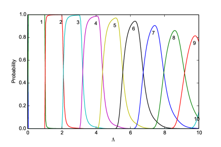
Figure 2: Probability to have $\nu$ excitation considering the microcanonical ensemble as a function of $\Lambda$ for $N=10^{4}$. The successive peaks correspond to increasing value of $\nu$. For example, $P(\nu=2)$ is close to 1 when $\Lambda$ is between 1 and 2.

From $\mathcal{N}(\nu)$, one easily computes the total number of allowed configurations $\mathcal{N}=\sum_{\nu}\mathcal{N}(\nu)$, the probability to have $\nu$ excitations in the sample $\mathcal{P}(\nu)=\mathcal{N}(\nu)/\mathcal{N}$ and the average excitation number $\langle\nu\rangle=\sum_{\nu}\nu\mathcal{P}(\nu)$ as well as its standard deviation $\left\langle\sigma_{\nu}\right\rangle$ as a function of $\Lambda$. The family of curves $\left\{\mathcal{P}(\nu),\nu=0,1,\dots\right\}$ is plotted on Fig. 2 as a function of $\Lambda$ for $N=10^{4}$ and on Fig. 8 for $N=10^{2}$; $\left\langle\nu\right\rangle$ and $\left\langle\sigma_{\nu}\right\rangle$ are represented on Fig. 3 as functions of $\Lambda$ for $N=10^{4}$. Our results show perfect quantitative agreement with BMFALA13 , as detailed in Appendix A

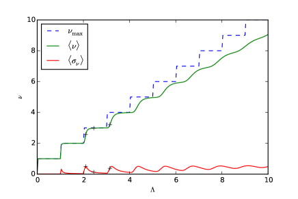
Figure 3: Average $\nu$ and standard deviation in the microcanonical predictions as a function of $\Lambda$ for $N=10^{4}$. The crosses correspond to the Monte-Carlo results from (BMFALA13, , fig 2c).

III.2 Spatial density of Rydberg excitations

We can go further in our analysis and compute how Rydberg excitations are distributed along the line in average. Calculations turn to be much easier in the limit of a homogeneous and continuous atomic distribution, of constant linear density $\delta\equiv\frac{1}{a}$ which is a good approximation of our model when $R_{b},L\gg a$.

Let us denote by $\mathcal{N}(\nu,l)$ the number of configurations with $\nu$ excitations on a line of length $l$ with the density $\delta$. We have

$$\forall l\geq 0,\;\mathcal{N}(0,l) =1$$

$$\forall l<0,\forall\nu,\;\mathcal{N}(\nu,l) =0$$

With these notations, $\mathcal{N}(\nu)=\mathcal{N}(\nu,L)$ and if $\nu>0$, the number of configurations with the leftmost excited atom at position $x$ is given by $\mathcal{N}(\nu-1,L-R_{b}-x)$. Integrating over $x$, we get the recurrence relation

$$\mathcal{N}(\nu+1,L)=\int_{0}^{L}dx\>\delta\>\mathcal{N}(\nu,L-R_{b}-x),$$ (6)

and

$$\mathcal{N}(\nu,L) =\frac{\delta^{\nu}}{\nu!}\left[l-(\nu-1)R_{b}\right]_{+}^{\nu}$$

$$=\frac{N^{\nu}}{\nu!}\left[1-\frac{\nu-1}{\Lambda}\right]_{+}^{\nu}$$ (7)

which is consistent with Eq. (5).

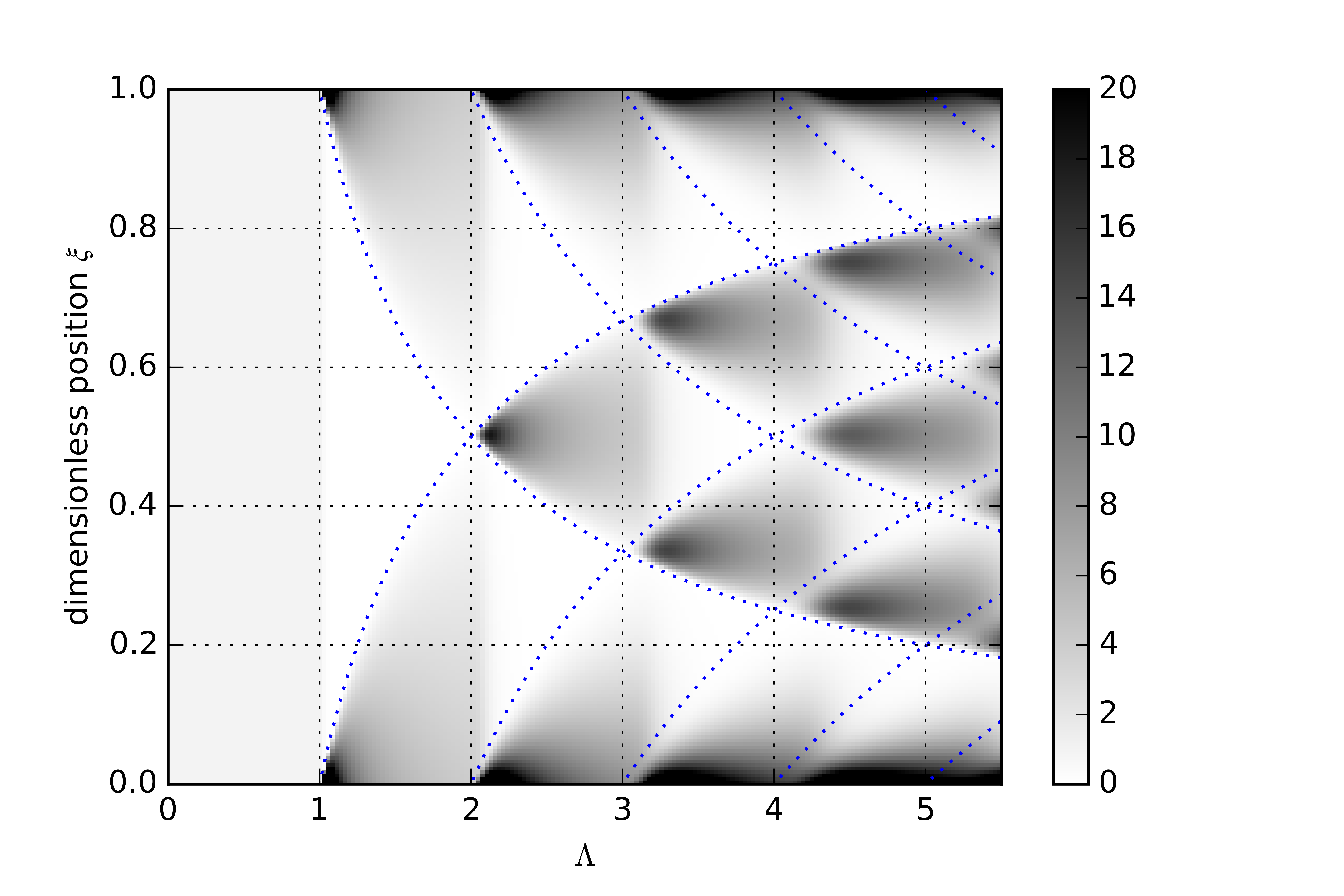
Figure 4: Probability distribution of Rydberg excitations along the chain as a function of $\Lambda$ and the position for $N=10^{4}$ atoms. This figure quantitatively reproduces the Monte-Carlo simulation of (BMFALA13, , fig 2a), as detailed in Appendix A.

The probability density to have the $n^{\text{th}}$ excited atom out of $\nu$ at the position $x$ is:

$$p(\nu,n,x)= \delta\>\frac{\mathcal{N}(n-1,x-R_{b})\times\mathcal{N}(\nu-n,L-R_{b}-x)}{\mathcal{N}(\nu)}$$

$$= \frac{\nu!\left[\xi-\tfrac{n-1}{\Lambda}\right]_{+}^{n-1}\left[1-\xi-\tfrac{\nu-n}{\Lambda}\right]_{+}^{\nu-n}}{\left(n-1\right)!\left(\nu-n\right)!\left[1-\tfrac{\nu-1}{\Lambda}\right]_{+}^{\nu}}$$ (8)

where we introduced the normalized dimensionless position $\xi\equiv\frac{x}{L}$. Note that it does not depend on $N$; as seen above, however, $N$ plays a role in the global probability for having $\nu$ excitations. This allows to plot the spatial distribution of excitation $\mathcal{P}\left(x\right)=\sum_{\nu}\sum_{n\leq\nu}p\left(\nu,n,x\right)$, as in Fig. 4 for $N=10^{4}$, which quantitatively agrees with the Monte-Carlo simulations provided in (BMFALA13, ; BMFALA13data, , fig 2a) (see Appendix A). The spatial distribution of excitations is also plotted in Fig. 9 (red curve) for $N=100$ and $\Lambda=1.5$.

IV Numerical and simplified analytical calculations of the thermalized state

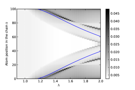
Figure 5: : Numerically computed probability distribution $\mathcal{P}_{k}$ of Rydberg excitations along the chain, as a function of $\Lambda$ and the position (see section IV.1) for $N=100$ atoms. The blue curve is the predicted position of the excitation peak by our simplified analytical treatment.

In this section, we present the results we obtained through a direct numerical calculation of the thermalized state averages and recover some of their interesting features through approximately diagonalizing the Hamiltonian in a conveniently truncated basis.

IV.1 Numerical calculation of the thermalized state

Our numerical method consists in time-averaging the observables of interest: if the average is performed on a very long (ideally infinite) time, the obtained average must indeed coincide with the thermalized value. Due to computational complexity, we restricted our study to a modest system of $N=100$ atoms equally spaced along the chain. Even with this relatively small value of $N$, the dimension $2^{N}$ of the complete Hilbert space makes the full dynamical treatment intractable. We therefore restricted ourselves to the regime $\Lambda<2$, i.e. the chain is shorter than two Rydberg radii ($L\leq 2R_{b}$) and the maximum number of excitations distributed along the chain is $2$. We only need to take into account the states allowed by the Rydberg blockade whose number is given by Eq. (7): $\sum_{\nu\leq 2}\mathcal{N}(\nu)\simeq\mathcal{N}(\nu=2)=\frac{N^{2}}{2}\left[1-\frac{1}{\Lambda}\right]_{+}^{2}$. We generate this set of allowed states through an arborescent search starting from $\left|\varnothing\right\rangle$ and adding allowed excitations.

In this subspace, we numerically diagonalize the Hamiltonian of Eq. (3), yielding the (possibly degenerate) eigenenergies $E_{n}$ and the associated eigenvectors $\ket{\psi_{n}^{\left(\alpha_{n}\right)}}$ where $\alpha_{n}=1\dots d_{n}$, $d_{n}$ are the degeneracy index of the eigenenergy $E_{n}$. Fig. 6 presents the numerical results of the diagonalization of $H$: more explicitly, the red curve shows the absolute value $\left|E_{n}\right|$ versus the rank of the corresponding eigenvectors $\ket{\psi_{n}^{\left(\alpha_{n}\right)}}$, arranged in increasing order of their eigenenergy; the blue curve represents the energy difference between two successive eigenvectors and therefore allows to check degeneracy. We take as a numerical criterion that two energies coincide when their difference is less than $10^{-13}\Omega$, consistent with the precision of IEEE 754 floating-point arithmetics. One first observes a wide central area corresponding to the highly degenerate eigenenergy $E\approx 0$; in addition, on both sides of the spectrum, there exist two pairs of eigenstates with degenerate energies.

If the system is initially prepared in $\ket{\Psi\left(0\right)}\equiv\sum_{n,\alpha_{n}}c_{n}^{\alpha_{n}}\ket{\psi_{n}^{\left(\alpha_{n}\right)}}$, its state at time $t$ is given by $\ket{\Psi\left(t\right)}=\sum_{n,\alpha_{n}}c_{n}^{\alpha_{n}}e^{-\mathrm{i}\frac{E_{n}}{\hbar}t}\ket{\psi_{n}^{\left(\alpha_{n}\right)}}$. The time-averaged probability $\mathcal{P}_{k}$ to have a Rydberg excitation in site $k$ is therefore given by $\mathcal{P}_{k}=\mathrm{Tr}\left[\bar{\rho}\sigma_{rr}^{\left(k\right)}\right]$ where the average state $\bar{\rho}$ is

$$\bar{\rho} =\overline{\left|\Psi\left(t\right)\right\rangle\left\langle\Psi\left(t\right)\right|}$$

$$=\sum_{m,\alpha_{m}}\sum_{n,\beta_{n}}c_{m}^{\alpha_{m}}\left(c_{n}^{\beta_{n}}\right)^{*}\left|\psi_{m}^{\left(\alpha_{m}\right)}\right\rangle\left\langle\psi_{n}^{\left(\beta_{n}\right)}\right|\times\overline{e^{-\mathrm{i}\frac{E_{m}-E_{n}}{\hbar}t}}$$

$$=\sum_{n,\alpha_{n},\beta_{n}}c_{n}^{\alpha_{n}}\left(c_{n}^{\beta_{n}}\right)^{*}\left|\psi_{n}^{\left(\alpha_{n}\right)}\right\rangle\left\langle\psi_{n}^{\left(\beta_{n}\right)}\right|.$$ (9)

We have used the time average $\overline{e^{-\mathrm{i}\frac{E_{m}-E_{n}}{\hbar}t}}=\delta_{mn}$ to simplify the double sum.

The probability distribution $\mathcal{P}_{k}$ is represented on Fig. 5 as a function of $\Lambda$. For $\Lambda\gtrsim 1.2$, two one-atom-wide black lines appear, revealing a strong localization of Rydberg excitations. In the next subsection, we account for this phenomenon through the approximate diagonalization of the Hamiltonian in a conveniently truncated basis.

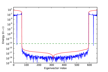
Figure 6: In red: $|E_{n}|$ versus $\left(n,\alpha_{n}\right)$ with $\Lambda=1.5$ (eigenstates are arranged in increasing order of their eigenenergy). In blue: difference between two successive eigenvalues, i.e. $\left|E_{n+1}-E_{n}\right|$. The dashed line shows the degeneracy limit: below this line, any values can be assumed to be zero, up to numerical artifacts (see text).

IV.2 Simplified analytical treatment

We are now looking for a simple description of the system which would retain the basic physical features of the model, in particular the localization effect observed in the previous subsection. To this end, we shall try and restrict the basis of the whole Hilbert space to only the relevant states, i.e. those which get significantly populated during the evolution.

As a first try, we consider the four-dimensional basis $\left\{\left|\varnothing\right\rangle,\left|\phi_{1}\right\rangle,\left|\phi_{2}\right\rangle,\left|\phi_{3}\right\rangle\right\}$ defined by

$$\left|\phi_{1}\right\rangle \equiv\frac{H\left|\varnothing\right\rangle}{\left\|H\left|\varnothing\right\rangle\right\|}$$ (10)

$$\left|\phi_{2}\right\rangle \equiv\frac{\Pi_{2}H\left|\phi_{1}\right>}{\left\|\Pi_{2}H\left|\phi_{1}\right>\right\|}=\frac{\Pi_{2}H^{2}\left|\varnothing\right\rangle}{\left\|\Pi_{2}H^{2}\left|\varnothing\right\rangle\right\|}$$ (11)

$$\left|\phi_{3}\right\rangle \equiv\frac{H\left|\phi_{2}\right>}{\left\|H\left|\phi_{2}\right>\right\|}=\frac{H\Pi_{2}H^{2}\left|\varnothing\right\rangle}{\left\|H\Pi_{2}H^{2}\left|\varnothing\right\rangle\right\|}$$ (12)

where $\Pi_{2}$ denotes the projector onto the subspace of states with exactly two Rydberg excitations. The diagonalization of $H$ in this subspace yields four eigenstates $\left|\psi_{i=1,2}^{s=\pm}\right\rangle$ and eigenenergies $\pm E_{i=1,2}$, such that $H\left|\psi_{i}^{s}\right\rangle=s\times E_{i}\left|\psi_{i}^{s}\right\rangle$, whose explicit expressions can be found in Appendix C. We conventionally choose $E_{2}\geq E_{1}\geq 0$. The eigenenergies $E_{i}$ are plotted as functions of $\Lambda$ on Fig. 7. Note that for $\Lambda>1$, all four eigenenergies $\pm E_{i=1,2}$ take different values, there is hence no degeneracy.

Since the eigenstates $\left|\psi_{i}^{s}\right\rangle$ describe configurations where excitations are delocalized (see Appendix D), the probability $\mathcal{P}_{k}$ computed from the time-averaged state Eq. (9)

$$\bar{\rho} =\sum_{i=1,2}\sum_{s=\pm}\left|c_{i}^{s}\right|^{2}\left|\psi_{i}^{s}\right\rangle\left\langle\psi_{i}^{s}\right|$$

will not exhibit the observed strong localization effect. Note that the four eigenstates $\left|\psi_{i=1,2}^{s=\pm}\right\rangle$ contribute to the statistical mixture $\bar{\rho}$ with the respective weights $\left|c_{i}^{s}\right|^{2}\equiv\left|\Braket{\psi_{i}^{s}}{\Psi(0)}\right|^{2}$ determined by the initial state vector $\ket{\Psi(0)}=\ket{\varnothing}$.

To correctly account for the observed localization phenomenon, we must therefore slightly extend the basis. To this end, we consider the family of states $\left\{\ket{\varphi_{k=1,\dots,N-n_{b}-1}^{s=\pm}}\right\}$ defined by

$$\Ket{\varphi_{k=1,\dots,N-R_{b}-1}^{\pm}}\equiv\frac{\ket{\Phi_{k}^{\left(1\right)}}\pm\ket{\Phi_{k}^{\left(2\right)}}}{\sqrt{2}}$$ (13)

with

$$\left|\Phi_{k}^{\left(1\right)}\right\rangle \equiv\frac{\left|k\right\rangle+\left|N-k\right\rangle}{\sqrt{2}}$$

$$\left|\Phi_{k}^{\left(2\right)}\right\rangle \equiv\sum_{l=0}^{N-n_{b}-k-1}\frac{\left|k,N-l\right\rangle+\left|N-k,l\right\rangle}{\sqrt{2\left(N-n_{b}-k\right)}}$$

Note that $\ket{\Phi_{k}^{\left(1\right)}}$ describes a configuration with exactly one Rydberg excited atom, localized either at position $k$ or $\left(N-k\right)$; $\ket{\Phi_{k}^{\left(2\right)}}$ describes a configuration with two Rydberg excitations, one being localized in $k$ or $\left(N-k\right)$ while the other is fully delocalized along the chain. The states $\left|\varphi_{k}^{s}\right\rangle$ are therefore coherent superpositions of states with either one or two excitations, one being localized with certainty either at position $k$ or $\left(N-k\right)$.

The states $\left|\varphi_{k}^{s}\right\rangle$ are found to be approximately orthogonal to $\left|\psi_{k}^{s}\right\rangle$, i.e.

$$\left\langle\varphi_{k}^{s}\middle|\psi_{k^{\prime}}^{s^{\prime}}\right\rangle=O\left(\frac{1}{\sqrt{N}}\right).$$

They are, moreover, only very weakly coupled to $\left|\psi_{k}^{s}\right\rangle$ by the Hamiltonian, i.e.

$$\left\langle\varphi_{k}^{s}\middle|H\middle|\psi_{k^{\prime}}^{s^{\prime}}\right\rangle=O\left(\frac{1}{\sqrt{N}}\right).$$ (14)

Finally, for any $k=1,\dots,\left(N-R_{b}-1\right)$ and $s=\pm$, one has

$$\left\langle\varphi_{k}^{s}\left|H\right|\varphi_{k}^{s}\right\rangle=s\times\varepsilon_{k}.$$

The expression of $\varepsilon_{k}$ is given in Appendix D. Fig. 7 shows the quasi-continuum formed by the different $\varepsilon_{k}$’s plotted as functions of $\Lambda$.

If the system starts in a superposition of $\ket{\Psi_{k}^{s}}$, i.e. $\ket{\psi\left(0\right)}=\sum_{k,s}c_{k}^{s}\ket{\psi_{k}^{s}}$, one could be tempted, due to Eq. (14), to assume that none of the states $\ket{\varphi_{k}^{s}}$ ever gets substantially populated and to discard the whole family $\left\{\ket{\varphi_{k}^{s}}\right\}$ from our description. This would actually be incorrect: it may indeed happen that, for a given $k=K$, $\left|\varphi_{K}^{s}\right\rangle$ becomes resonant with $\left|\psi_{1}^{s}\right\rangle$, i.e. $\varepsilon_{K}=E_{1}$ (as can be checked on Fig. 7, such a resonance exists only for $\Lambda\geq\frac{7}{6}$; in Appendix D, this result is also analytically deduced from the expressions of $E_{1}$ and $\varepsilon_{k}$). In that case, though very weak, the coupling term $\left\langle\varphi_{K}^{s}\left|H\right|\psi_{1}^{s}\right\rangle$ strongly mixes the states $\left|\varphi_{K}^{s}\right\rangle$ and $\left|\psi_{1}^{s}\right\rangle$ and the two vectors $\left|\varphi_{K}^{s=\pm}\right\rangle$ must be adjoined to the previous set $\left\{\left|\psi_{i=1,2}^{s=\pm}\right\rangle\right\}$. In this subspace, the six eigenvectors of the Hamiltonian now read

$$\left\{\left|\chi_{\pm}^{s=\pm}\right\rangle\equiv\frac{\left|\psi_{1}^{s}\right\rangle\pm\left|\varphi_{K}^{s}\right\rangle}{\sqrt{2}},\left|\chi_{0}^{s=\pm}\right\rangle\equiv\left|\psi_{2}^{s}\right\rangle\right\}$$

and the energy degeneracy is lifted. An initial state of the form $\ket{\Psi(0)}=\sum_{k,s}c_{k}^{s}\ket{\psi_{k}^{s}}$ now has components on the six new eigenvectors, i.e. $\ket{\Psi(0)}=\sum_{r=\pm,0}\sum_{s=\pm}d_{r}^{s}\ket{\chi_{r}^{s}}$ and therefore the time-averaged state

$$\bar{\rho} =\sum_{r=\pm,0}\sum_{s=\pm}\left|d_{r}^{s}\right|^{2}\left|\chi_{r}^{s}\right\rangle\left\langle\chi_{r}^{s}\right|$$ (15)

now contains a highly localized component, on the atom at position $K$ or $\left(N-K\right)$. Accordingly, the probability distribution $\mathcal{P}_{k}$ exhibits a strongly peaked behavior at $k=K,\left(N-K\right)$. This localization phenomenon is in good qualitative agreement with what we observe with the full simulation: in particular, the appearance of the localization lines indeed happens when $\Lambda\approx\frac{7}{6}$ (see Fig. 5). This validates the simplified analytical treatment we have just carried out which indeed seems to retain the main physical ingredients of the system and its evolution.

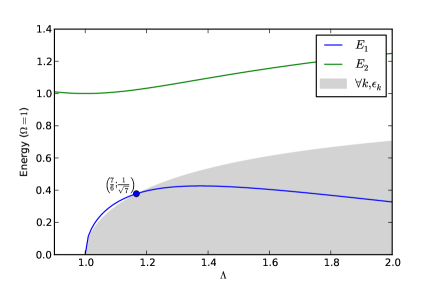
Figure 7: $E_{1},E_{2}$ and $\varepsilon_{k}$ as functions of $\Lambda$, computed by our simplified analytical treatment for $N=100$. The values of $\varepsilon_{k}$ form a quasi-continuum. As discussed in the text, localization peaks arise when a resonance takes place,i.e. when there exists a value $k=K$ such that $\varepsilon_{K}=E_{1}$. This happens for $\Lambda\geq\frac{7}{6}$ as can be shown analytically (see Appendix D) and graphically checked on the present Figure.

V Discussion

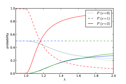
Figure 8: Probability to have $\nu$ excitations as a function of $\Lambda$, with $N=100$, according to the microcanonical predictions (red), our numerical simulation (green) and the analytical treatment (blue).

Figure 9: Spatial distribution of excitations at $\Lambda=1.5$, with $N=100$, according to the microcanonical predictions (red), our numerical simulation (green) and the analytical model (blue).

This section is devoted to the comparison of the results obtained above following the different approaches and to discussions on their differences.

Fig. 8 displays plots of the probability $\mathcal{P}(\nu)$ to have $\nu$ Rydberg excitations in the sample, as a function of $\Lambda$ (for $0.9\leq\Lambda\leq 2$), calculated according to: i) the microcanonical hypothesis (Sec. III); ii) the full simulation of the system (Sec. IV.1); iii) the approximate diagonalization of $H$ in a reduced $6$-dimensional Hilbert space (Sec. IV.2). While the schemes ii) and iii) yield very similar results (as expected), assumption i) induces quite different behaviors. The same comparison can be performed on the spatial probability distribution $\mathcal{P}_{k}$ which is displayed on Fig. 9. Again, the shapes obtained via schemes ii) and iii) are in very good qualitative agreement: in both cases, one observes two localization peaks on a “background curve”, which coincide satisfactorily. (Note that, according to our calculations, excitations are more likely to be localized at the borders). The spatial probability distribution obtained according to assumption i) differs strongly: no excitation localization effect is observed and the background curve is far from what is observed in the full simulation.

The discrepancies observed above can be partly explained by the following “parity balance property” established in Appendix B: for any eigenstate $\ket{\psi}$ of the Hamiltonian $H$ of nonzero energy, the projections $\left|\psi_{\text{odd}}\right\rangle$ and $\left|\psi_{\text{even}}\right\rangle$ onto the orthogonal and plementary subspaces $\mathcal{H}_{\text{odd}}$ and $\mathcal{H}_{\text{even}}$, respectively spanned by the states with an odd and even number of Rydberg excitations, have the same norm, i.e. $\left|\psi\right\rangle=\left|\psi_{\text{odd}}\right\rangle+\left|\psi_{\text{even}}\right\rangle$ with $\left\|\left|\psi_{\text{odd}}\right\rangle\right\|=\left\|\left|\psi_{\text{even}}\right\rangle\right\|=\frac{1}{\sqrt{2}}$. This property conflicts directly with the microcanonical predictions according to which the probability to have $\nu<\nu_{\max}$ excitations is negligible compared to the probability to have the maximum number of excitations. For example, suppose $\nu_{\max}=1$, the microcanonical ensemble implies that $P(\nu=0)=\frac{1}{1+N}$ and $P(\nu=1)=\frac{N}{1+N}$. By contrast, the parity balance property implies $P(\nu=0)=P(\nu=1)=0.5$. Furthermore, one can see that in Fig. 2, each time one of the probability curve is above $\frac{1}{2}$, the parity balance condition is therefore impossible to fulfill. In almost all cases, the even/odd parity balance property and the simple microcanonical approach presented in Sec. III disagree.

The inaccuracy of the predictions deduced from the microcanonical assumption can also be explained by the choice of $\left|\varnothing\right\rangle$ as initial state: the low connectivity of this state to the rest of the Hilbert space constitutes indeed a strongly limiting factor to the thermalization process OML10 . In particular, the vaccum state being symmetric as well as the Hamiltonian, the system remains in a symmetric state during its evolution. The direct application of the microcanonical assumption, taking into account all the states which are allowed by the Rydberg blockade, is therefore incorrect : for a proper use of the microcanonical hypothesis, one should actually take this extra symmetry selection rule into consideration and count only the accessible, i.e. symmetric, states. Note that the vacuum state is the natural starting point from an experimental perspective to study the build-up of excitations and is therefore widely used AL12 ; BMFALA13 .

Another choice of initial state can actually be considered. Starting with a random initial state, Ates et al. AGL12 showed that in the regime of strong nearest neighbor interaction ($\Lambda>\frac{N}{2}$), the dynamics of the system is well described by the microcanonical ensemble. In the regime studied in the present article, $\Lambda\ll N$, a similar random choice of initial state leads to an essentially “frozen evolution” as seen by the following dimensionality arguments. From Eq. (7), the number of states containing at most $\nu_{\max}-1$ excitations is $\propto N^{\nu_{\max}-1}$ and the dimension of the generated subspace $\mathcal{H}_{\nu\leq\nu_{\max}-1}$ is a small fraction $O(\frac{1}{N})$ of the dimension of the total Hilbert space $\mathcal{H}$. As $N$ increases, the Hilbert space is therefore essentially composed by states containing $\nu_{\max}$ excitations. Furthermore, since all eigenvectors of $H$ with non-zero eigenvalue follow the parity balance property,

$$\text{dim}(\mathcal{H}\setminus\text{ker}(H)) \leq 2\min\left(\text{dim}(\mathcal{H}_{\text{even}}),\text{dim}(\mathcal{H}_{\text{odd}})\right)$$

$$\sim 2\text{dim}\left(\mathcal{H}_{\nu=\nu_{\max}-1}\right)$$

$$\sim O\left(N^{\nu_{\max}-1}\right)$$

As a consequence, the Hilbert space is mainly spanned by the states in $\mathrm{ker}\left(H\right)$ with $\nu_{\max}$ excitations. This can be seen, for example, on Fig. 6. Therefore, the projector on $\text{ker}(H)$ is a “gentle” operator W99 for the ensemble of states picked uniformly at random: with high probability, a state from this ensemble will have a large component on $\text{ker}(H)$ and its evolution will essentially be “frozen”, which contradicts the microcanonical predictions.

Conversely, if one chooses the initial state in the $\mathcal{H}_{\nu\leq\nu_{\max}-1}$ subspace, the system will not explore $\text{ker}(H)$: the dimensionality of the actual microcanonical ensemble is therefore again much less than the number of states allowed by the Rydberg blockade. Note that this initial state choice is a natural generalization of $\ket{\varnothing}$ to study the buildup of excitations.

VI Conclusion

In the present article, we studied the dynamics of a 1D-Rydberg ensemble in the regime of at most 2 excitations. In the same conditions as in AL12 ; BMFALA13 , we tested the validity of the microcanonical predictions and found it cannot be used straightforwardly to account for the thermalization process which occurs in this particular regime. Though the observed discrepancies can be related to our specific choice of initial state and its particular symmetry properties, we also proved, by an argument involving the dimension of the kernel of the Hamiltonian, that the same restriction holds for a randomly chosen initial state.

Further investigations are needed to better understand when and how to apply the (micro)canonical predictions. In particular, the results presented here all rely on the hardcore sphere assumption. Refining the model and considering the full Rydberg-Rydberg interaction Hamiltonian Eq. (1) might actually change our conclusions and make the microcanonical assumption more adapted, as shown in LOG10 . Indeed, in that case, all states become, strictly speaking, allowed, though more or less accessible, and the connectivity accordingly increases between states of the Hilbert space. Moreover, as suggested by our discussion, the systematic study of symmetry properties of the system at stake, as well as the selection rules they impose, appears to be a crucial point in the proper application of microcanonical assumption.

Appendix A Quantitative agreement of our analytical treatment and Bettelli et al.’s Monte-Carlo Simulation

In this appendix, we compare our analytical treatment of the microcanonical hypothesis with the Monte-Carlo results published by Bettelli et al. in BMFALA13 .

On their Fig. 2, Bettelli et al. give the average number of excitation $\braket{\nu}$ and its standard deviation $\sqrt{\braket{\Delta\nu^{2}}}$ for $\Lambda\in\{2.1,2.45,3.15\}$. These data points correspond to the crosses on Fig. 3 and fall on the corresponding curves computed according to our analytical treatment. For 5 of these 6 values, our results are indeed identical to the two published decimals. The 6th value is the standard deviation for $\Lambda=3.15$, where we obtain $\sqrt{\braket{\Delta\nu^{2}}}=0.41$, to be compared to $0.38$. This deviation is small, and we therefore consider the results to be effectively identical.

Figure 10: Root-mean-square difference between the Monte-Carlo result of BMFALA13 and the analytical Eq. (8) as a function of $\Lambda$.

Figure 11: Difference between the Monte-Carlo result of BMFALA13 and the analytical result Eq. (8). On the dotted lines, either $\xi$ or $1-\xi$ is an integer multiple of $\frac{1}{\Lambda}$.

We compared the spatial distribution of excitations of Fig. 4 to the data BMFALA13data kindly provided bay the authors of BMFALA13 . This data-set was obtained with a Monte-Carlo simulation with $N=10^{4}$ atoms and $N_{\text{rep.\@}}=5\times 10^{4}$ repetitions, using $N_{\text{bin}}=100$ bins and a normalization to an average excitation density of 1.

We plotted the Monte-Carlo simulation and our data, computed from Eq. (8), using the same normalization and we were unable to visually see any difference by blinking between the two plots on our computer screen. More quantitatively, we plotted the root-mean-square difference between the two sets of data for each value of $\Lambda$ on Fig. 10, as well as the pixel by pixel difference on Fig. 11.

When $\Lambda<1$, the probability to have one excitation in any given bin is $\frac{1}{N_{\text{bin}}}$; the expected value of this root-mean-square difference as well as the standard deviation of the difference should then be $\sqrt{\frac{N_{\text{bin}}}{N_{\text{rep}}}}=\sqrt{\frac{1}{500}}\simeq 0.045$. When $\Lambda\geq 1$, no strong localization is expected, and this calculation should therefore give a correct order of magnitude, both for the root-mean-square difference for a given $\Lambda$ and for the pixel by pixel fluctuations. This is quantitatively consistent with the results.

Furthermore, the main deviations in both graphs can be explained by the different approximations in plotting each pixel : for the Monte-Carlo simulation BMFALA13data , the value of a pixel of coordinates $(\Lambda,\xi)$ corresponds do an average over the segment $\left[\xi,\xi+\frac{1}{N_{\text{bin}}}\right)$, while, for the analytical formula (8), we computed its value at the center of the pixel, i.e. for $\xi+\frac{1}{2N_{\text{bin}}}$. The latter approximation, taken for the sake of simplicity, is only justified when Eq. (8) is reasonably flat. The main deviations seem indeed to be localized where the latter approximation is not justified, i.e. when the excitations are concentrated in a few narrow peaks, or where either $\xi$ or $1-\xi$ is an integer multiple of $\frac{1}{\Lambda}$.

Our analytical treatment of the microcanonical ensemble assumption is therefore quantitatively consistent with the Monte-Carlo simulation in BMFALA13 ; BMFALA13data .

Appendix B Parity balance property

Our analytical model has been build according to an observation on the structure of $H$: the parity balance property presented in Sec. V. The Hilbert space $\mathcal{H}$ can be decomposed into 2 orthogonal subspaces containing an even/odd number of excitations: $\mathcal{H}=\mathcal{H}_{\text{even}}\oplus\mathcal{H}_{\text{odd}}$. Since $H$ either removes or adds an excitation, its effect on a state containing an even (resp. odd) number of excitations will change the parity of its number of excitations to an odd (resp. even) value. From this, we can deduce that the subspaces $\mathcal{H}_{\text{even}}$ and $\mathcal{H}_{\text{odd}}$ are stable under the application of $H^{2}$. $H^{2}$ is therefore in the form:

$$H^{2}=\begin{pmatrix}H^{2}_{\text{even}}&0\\ 0&H^{2}_{\text{odd}}\\ \end{pmatrix}$$ (16)

Our analytical treatment is based on the diagonalization of $H^{2}_{\text{even}}$ and $H^{2}_{\text{odd}}$ to obtain the eigenstates of $H$. In particular, the eigenstates of $H$ follow this even/odd decomposition and can be written as $\Ket{\Psi}=\Ket{\Psi_{\text{even}}}+\Ket{\Psi_{\text{odd}}}$ with $\Ket{\Psi_{\text{even}/\text{odd}}}=\Pi_{\text{even}/\text{odd}}\Ket{\Psi}$ with $\Pi_{\text{even}/\text{odd}}$ being the projector on $\mathcal{H}_{\text{even}/\text{odd}}$. Using the orthogonality of $\Ket{\Psi_{\text{even}}}$ and $\Ket{\Psi_{\text{odd}}}$, a short calculation from $H\Ket{\Psi_{\text{even}/\text{odd}}}=E\Ket{\Psi_{\text{odd}/\text{even}}}$ leads to either $E=0$, or $\left\|\Ket{\Psi_{\text{even}}}\right\|=\left\|\Ket{\Psi_{\text{odd}}}\right\|=\frac{1}{\sqrt{2}}$, i.e. all non zero energy eigenstates are equally weighted between even and odd parts.

If $\Lambda<2$, it is straightforward to see that all $E=0$ eigenstates are orthogonal to $\Ket{\varnothing}$. If the initial state is $\Ket{\varnothing}$, the average probability to have an even (or odd) number of excitations is therefore exactly $\frac{1}{2}$.

Appendix C Diagonalization of $H^{2}$

Here, we present a more detailed version of the diagonalization of $H^{2}$ showed in Sec. IV.2 using its even/odd decomposition described by Eq. (16) in Appendix B. The states defined by Eqs. (10),(11) and (12) have the following explicit formulations:

$$\left|\phi_{1}\right\rangle =\frac{1}{\sqrt{N}}\sum_{k=0}^{N-1}\Ket{k}$$

$$\left|\phi_{2}\right\rangle =Z_{2}\sum_{k=0}^{N-n_{b}-1}{\sum_{l=k+n_{b}}^{N-1}{2\Ket{k,l}}}$$

$$\left|\phi_{3}\right\rangle =Z_{3}\left(\sum_{k=0}^{N-n_{b}-1}{(N-n_{b}-k)\Ket{k}}+\sum_{l=n_{b}}^{N-1}{(l-n_{b})\Ket{l}}\right)$$

When $N\gg 1$, the sums involved in the computation of $\Braket{\phi_{2}}{\phi_{2}}$ and $\Braket{\phi_{3}}{\phi_{3}}$ can easily be approximated by integrals, and the normalization factors are therefore:

$$Z_{2} \simeq\frac{\sqrt{3/2}}{(N-n_{b})^{3/2}}$$ (17)

$$Z_{3} \simeq\frac{1}{\sqrt{2}(N-n_{b})}$$ (18)

$H^{2}_{\text{even}}$ can be expressed in the basis $\{\Ket{\varnothing},\Ket{\phi_{2}}\}$:

$$H^{2}_{\text{even}}=\Omega^{2}N\begin{pmatrix}1&\rho\sqrt{2}\\ \rho\sqrt{2}&\frac{4}{3}\rho\\ \end{pmatrix}$$

with $\rho=\frac{N-n_{b}}{N}\simeq 1-\frac{1}{\Lambda}$. The eigenvalues are

$$E^{2}_{\text{even},1} =\Omega^{2}N\frac{4\rho+3-\sqrt{88\rho^{2}-24\rho+9}}{6}$$ (19)

$$E^{2}_{\text{even},2} =\Omega^{2}N\frac{4\rho+3+\sqrt{88\rho^{2}-24\rho+9}}{6}$$ (20)

for respectively $\Ket{E^{2}_{\text{even},1}}$ and $\Ket{E^{2}_{\text{even},2}}$.

$H^{2}_{\text{odd}}$ can be expressed in the orthonormal basis $\{\Ket{\phi_{1}},\Ket{\phi_{1}^{\perp}}=Z_{1}^{\perp}(\Ket{\phi_{3}}-\Braket{\phi_{1}}{\phi_{3}}\Ket{\phi_{1}})\}$ with $Z_{1}^{\perp}=\frac{1}{\sqrt{1-\frac{3\rho}{2}}}$.

$$H^{2}_{\text{odd}}=\Omega^{2}N\begin{pmatrix}1+2\rho^{2}&2\rho^{3/2}\sqrt{\frac{2}{3}-\rho}\\ 2\rho^{3/2}\sqrt{\frac{2}{3}-\rho}&\frac{4}{3}\rho-2\rho^{2}\\ \end{pmatrix}$$

Diagonalizing $H^{2}_{\text{odd}}$ in the same way, we find its eigenvalues $E^{2}_{\text{odd},i}=E^{2}_{\text{even},i}=E^{2}_{i}$ corresponding to the eigenvectors $\Ket{E^{2}_{\text{odd},i}}$ with $i=1,2$.

Each subspace with eigenvalue $E^{2}_{i=1,2}$ has dimension 2 and is thus generated by $\frac{\Ket{E^{2}_{\text{even},i}}+e^{i\phi}\Ket{E^{2}_{\text{odd},i}}}{\sqrt{2}}$ and $\frac{\Ket{E^{2}_{\text{even},i}}-e^{i\phi}\Ket{E^{2}_{\text{odd},i}}}{\sqrt{2}}$. Let us fix the arbitrary relative phase $\phi$ to 0 by the equation:

$$H\Ket{E^{2}_{\text{even},i}}=\sqrt{E^{2}_{i}}\Ket{E^{2}_{\text{odd},i}}.$$

Combining it with $H^{2}\Ket{E^{2}_{\text{even},i}}=E^{2}_{i}\Ket{E^{2}_{\text{even},i}}$ gives

$$H\Ket{E^{2}_{\text{odd},i}}=\sqrt{E^{2}_{i}}\Ket{E^{2}_{\text{even},i}}.$$

We trivially define the 4 eigenvalues of $H$ by $E^{s=\pm}_{i=1,2}=s\times E_{i=1,2}=s\times\sqrt{E^{2}_{i=1,2}}$ of the 4 eigenvectors $\ket{\psi^{\pm}_{i=1,2}}=\frac{\ket{E^{2}_{\text{even},i}}+s\times\Ket{E^{2}_{\text{odd},i}}}{\sqrt{2}}$.

Appendix D Localization of excitations

Now, we present specifically our analytical treatment of the localization effects observed in Fig. 5. The states $\Ket{\phi_{1}}$, $\Ket{\phi_{2}}$ and $\Ket{\phi_{3}}$ used in Sec. IV.2 are delocalized. To account for the very narrow localization of excitations (1 atom wide), we complete the four states $\ket{\psi^{\pm}_{i=1,2}}$ with the family of states $\ket{\varphi_{k}^{s=\pm}}$ defined in Eq. (13).

For large $N$, those states are approximate eigenstates of $H$ with eigenvalues $s\times\varepsilon_{k}=s\times\Omega\sqrt{N-n_{b}-k}$:

$$H\Ket{\varphi_{k}^{s=\pm}}=s\times\Omega\sqrt{N-n_{b}-k}\Ket{\varphi_{k}^{s=\pm}}+O\left(\frac{1}{\sqrt{N}}\right).$$ (21)

As seen in section IV.2, for a particular value $K$, the state $\Ket{\varphi_{K}^{s=\pm}}$ has the same energy as the collective excitation state $\Ket{\psi^{s}_{1}}$. This resonance can only exist if

$$E_{1}\leq\varepsilon_{0}\Leftrightarrow\Omega\sqrt{N\frac{4\rho+3-\sqrt{88\rho^{2}-24\rho+9}}{6}}\leq\Omega\sqrt{N\rho}$$ (22)

This inequality holds when $\Lambda\geq\frac{7}{6}$.

The small coupling between those states lifts this degeneracy by adding an energy shift $\pm\delta$ to the new eigenvectors $\Ket{\chi^{s=\pm}_{\pm}}=\frac{\Ket{\varphi_{K}^{s}}\pm\Ket{\psi^{s}_{1}}}{\sqrt{2}}$ of energy $s\times E_{1}\pm\delta$. This degeneracy allows us to keep only the diagonal terms in the density matrix after time averaging. Furthermore, when $\ket{\Psi(0)}$ is reasonably delocalized state, like e.g. $\ket{\varnothing}$, we have $\Braket{\chi^{s}_{\pm}}{\Psi(0)}=\frac{\Braket{\psi^{s}_{1}}{\Psi(0)}}{\sqrt{2}}+O(\frac{1}{\sqrt{N}})$. After time averaging, the density matrix contains only diagonal terms and one can deduce the density matrix:

$$\bar{\rho}=\left|\Braket{\psi^{+}_{2}}{\Psi(0)}\right|^{2}\left(\Ket{\psi^{+}_{2}}\Bra{\psi^{+}_{2}}+\Ket{\psi^{-}_{2}}\Bra{\psi^{-}_{2}}\right)+\frac{|\Braket{\psi^{-}_{1}}{\Psi(0)}|^{2}}{2}\left(\Ket{\psi^{-}_{1}}\Bra{\psi^{-}_{1}}+\Ket{\psi^{+}_{1}}\Bra{\psi^{+}_{1}}+\Ket{\varphi_{K}^{+}}\Bra{\varphi_{K}^{+}}+\Ket{\varphi_{K}^{-}}\Bra{\varphi_{K}^{-}}\right)$$ (23)

The average state $\bar{\rho}$ of the system is therefore a statistical mixture involving $\Ket{\psi^{+}_{2}}$ and $\Ket{\psi^{-}_{2}}$ weighted by $\left|\Braket{\psi^{+}_{2}}{\Psi(0)}\right|^{2}$ and the four states $\Ket{\psi^{-}_{1}}$, $\Ket{\psi^{+}_{1}}$,$\Ket{\varphi_{K}^{-}}$ and $\Ket{\varphi_{K}^{+}}$ weighted by $\tfrac{1}{2}{\left|\Braket{\psi^{-}_{1}}{\Psi(0)}\right|^{2}}$. This is the explicit form of the density matrix described by Eq. (15).

References

- (1) T.F. Gallagher, “Rydberg Atoms”, Cambridge University Press, Cambridge (1994).
- (2) M. Saffman, T. G. Walker, and K. Mølmer, “Quantum information with Rydberg atoms”, Rev. Mod. Phys. 82, 2313 (2010).
- (3) D. Jaksch, J. I. Cirac, P. Zoller, S.L. Rolston, R. Côté and M.D. Lukin, Phys. Rev. Lett. 85, 2208 (2000).
- (4) I. E. Protsenko, G. Reymond, N. Schlosser, and P. Grangier, Phys. Rev. A 65, 052301 (2002).
- (5) M. Saffman and T. G. Walker, Phys. Rev. A 72, 022347 (2005).
- (6) M. D. Lukin, M. Fleischhauer, R. Côté, L. M. Duan, D. Jaksch, J. I. Cirac, and P. Zoller, Phys. Rev. Lett. 87, 037901 (2001).
- (7) D. Tong, S. M. Farooqi, J. Stanojevic, S. Krishnan, Y. P. Zhang, R. Côté, E. E. Eyler, and P. L. Gould, Phys. Rev. Lett. 93, 063001 (2004).
- (8) K. Singer, M. Reetz-Lamour, T. Amthor, L. G. Marcassa, and M. Weidemüller, Phys. Rev. Lett. 93, 163001 (2004).
- (9) T. Cubel Liebisch, A. Reinhard, P. R. Berman, and G. Raithel, Phys. Rev. Lett. 95, 253002 (2005).
- (10) W. R. Anderson, J. R. Veale, and T. F. Gallagher, Phys. Rev. Lett. 80, 249 (1998).
- (11) T. Vogt, M. Viteau, J. Zhao, A Chotia, D. Comparat, and P. Pillet, Phys. Rev. Lett. 97, 083003 (2006).
- (12) E. Brion, A. S. Mouritzen et K. Mølmer, Phys. Rev. A 76, 022334 (2007).
- (13) E. Brion, K. Mølmer, M. Saffman, Phys. Rev. Lett. 99, 260501 (2007).
- (14) E. Brion, L. H. Pedersen, M. Saffman, K. Mølmer, Phys. Rev. Lett. 100, 110506 (2008).
- (15) B. Zhao, M. Mœller, K. Hammerer, and P. Zoller, Phys. Rev. A 81, 052329 (2010).
- (16) Y. Han, B. He, K. Heshami, C.-Z. Li, and C. Simon, Phys. Rev. A 81, 052311 (2010).
- (17) E. Brion, F. Carlier, V. M. Akulin and K. Mølmer, Phys. Rev. A 85, 042324 (2012).
- (18) K. J. Weatherill, C. S. Adams, Annual review of cold atoms and molecules 1, 301 (2013).
- (19) T. Peyronel, O. Firstenberg, Q.-Y. Liang, S. Hofferberth, A. V. Gorshkov, T. Pohl, M. D. Lukin and V. Vuletić, Nature 488, 57–60 (2012).
- (20) V. Parigi, E. Bimbard, J. Stanojevic, A. J. Hilliard, F. Nogrette, R. Tualle-Brouri, A. Ourjoumtsev, and Ph. Grangier, Phys. Rev. Lett. 109, 233602 (2012).
- (21) D. Maxwell, D. J. Szwer, D. Paredes-Barato, H. Busche, J. D. Pritchard, A. Gauguet, K. J. Weatherill, M. P. A. Jones, and C. S. Adams, Phys. Rev. Lett. 110, 103001 (2013).
- (22) I. Lesanovsky, B. Olmos, and J. P. Garrahan, Phys. Rev. Lett. 105 100603 (2010).
- (23) C. Ates and I. Lesanovsky, Phys. Rev. A 86, 013408 (2012)
- (24) S. Bettelli, D. Maxwell, T. Fernholz, C. S. Adams, I. Lesanovsky, C. Ates, “Exciton dynamics in emergent Rydberg Lattices", Phys. Rev. A 88, 043436 (2013).
- (25) S. Ji, C. Ates, J. P. Garrahan, and I. Lesanovsky, J. Stat. Mech.: Theory Expt. (2013) P02005.
- (26) C. Ates, J. P. Garrahan, and I. Lesanovsky, Phys. Rev. Lett. 108, 110603 (2012).
- (27) S. Bettelli, D. Maxwell, T. Fernholz, C. S. Adams, I. Lesanovsky, C. Ates, Raw data used to plot fig 2a of BMFALA13 , provided by S. Bettelli through private communication (2016).
- (28) B. Olmos, M. Müller and I. Lesanowsky, New Joural of Physics 12, 013024 (2010).
- (29) A. Winter, IEEE Transactions on Information Theory, 45 (7) 2481 (1999).