Towards 1/N corrections to deep inelastic scattering from the gauge/gravity duality

David Jorrin, Nicolas Kovensky, and Martin Schvellinger

IFLP-CCT-La Plata, CONICET and Departamento de Física, Universidad Nacional de La Plata. Calle 49 y 115, C.C. 67, (1900) La Plata, Buenos Aires, Argentina.

Abstract

$1/N^{2}$ corrections to deep inelastic scattering (DIS) of charged leptons from glueballs at strong coupling are investigated in the framework of the gauge/gravity duality. The structure functions $F_{1}$ and $F_{2}$ (and also $F_{L}$) are studied at subleading order in the $1/N^{2}$ expansion, in terms of $q^{2}$ and the Bjorken parameter $x$. The relevant type IIB supergravity one-loop diagrams (which correspond to DIS with two-hadron final states) are studied in detail, while $n$-loop diagrams (corresponding to DIS with $(n+1)$-hadron final states) are briefly discussed. The $1/N^{2n}$ and $\Lambda^{2}/q^{2}$ dependence of the structure functions is analyzed. Within this context two very different limits are considered: one is the large $N$ limit and the other one is when the virtual photon momentum transfer $q$ is much larger than the infrared confining scale $\Lambda$. These limits do not commute.

1 Introduction

The idea of the present work is to investigate $1/N^{2}$ corrections to DIS of charged leptons off glueballs at strong coupling by using the gauge/gravity duality. This corresponds to a DIS process where there are two-hadron final states. By using the optical theorem this is related to a forward Compton scattering (FCS) process with two-particle intermediate states, i.e. one-loop FCS Feynman diagrams. Moreover, we also consider $1/N^{2n}$ corrections to DIS (where $n$ is an integer), which corresponds to $(n+1)$-hadron final states, while in terms of FCS it is related to $(n+1)$-particle intermediate states, i.e. $n$-loop FCS Feynman diagrams.

In terms of the gauge/string duality Polchinski and Strassler studied scattering processes in the large $N$ limit both for hard scattering [1] and for DIS [2]. Further work related to DIS from the gauge/string duality includes [3, 4, 5, 6, 7, 8, 9, 10, 11, 12, 13, 14, 15, 16, 17, 18, 19, 20, 21]. For DIS in [2] the authors considered the structure functions of glueballs in the case when there is a single-hadron final state. In addition, they suggested that for two-hadron final states DIS can also be studied within the supergravity description. Thus, we will investigate type IIB supergravity loop corrections, in particular describing in detail one-loop corrections.

DIS of a charged lepton off a hadron is schematically shown in figure 1.

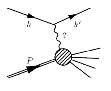
Figure 1: Schematic picture of DIS of a charged lepton with four-momentum $k$ off a hadron with four-momentum $P$, through the exchange of a virtual photon with four-momentum $q$.

The process involves a charged lepton with four-momentum $k$, which emits a virtual photon with four-momentum $q$. This probes the internal structure of a target hadron with initial four-momentum $P$. The scattering cross section of DIS is proportional to the contraction of a leptonic tensor, $l_{\mu\nu}$, described by using perturbative QED, and a hadronic tensor, $W_{\mu\nu}$, which is difficult to calculate since it involves soft QCD processes. At weak coupling, the parton model describes this process: the virtual photon interacts directly with one of the partons inside the hadron. At strong coupling, on the other hand, the parton model is not a suitable description and therefore a different strategy must be considered. We will use an approach based on the gauge/string duality and the methods developed in [2].

In general terms, from the theoretical point of view, there is a standard way to proceed in order to study the internal structure of hadrons. In fact, by using the optical theorem the DIS cross section is related to the matrix element of a product of two electromagnetic currents $J^{\mu}(x)\,J^{\nu}(0)$ inside the hadron, which corresponds to the FCS process. The product of these two currents can be written in terms of the operator product expansion (OPE), for an unphysical kinematical region (i.e. for $x\gg 1$). Then, by using dispersion relations it is possible to connect the above unphysical result with the physical DIS cross section. The matrix element of two electromagnetic currents inside the hadron is given by the tensor $T^{\mu\nu}$, which is defined as

$$T^{\mu\nu}=i\int d^{4}x\,e^{iq\cdot x}\,\langle P,h^{\prime}|{\hat{T}}(J^{\mu}(x)\,J^{\nu}(0))|P,h\rangle\,,$$ (1)

where $h$ and $h^{\prime}$ label the polarizations of the initial and final hadronic states. $\hat{T}$ indicates the time ordered product of the two currents. This tensor depends on $q^{2}$ and the Bjorken parameter defined as

$$x=\frac{-q^{2}}{2P\cdot q}\,,$$ (2)

being $0\leq x\leq 1$ its physical kinematical range, where $x=1$ corresponds to elastic scattering. Beyond the physical kinematical region, i.e. for $x>1$, it is possible to carry out the OPE of the tensor $T^{\mu\nu}$. This tensor is related by the optical theorem to the hadronic tensor

$$W_{\mu\nu}(P,q)=i\int d^{4}x\,e^{iq\cdot x}\langle P,h^{\prime}|[J_{\mu}(x),J_{\nu}(0)]|P,h\rangle\,.$$ (3)

Since we will focus on scalar glueballs, the hadronic tensor is given by

$$W_{\mu\nu}=F_{1}(x,q^{2})\left(\eta_{\mu\nu}-\frac{q_{\mu}q_{\nu}}{q^{2}}\right)+\frac{2x}{q^{2}}\,F_{2}(x,q^{2})\left(P_{\mu}+\frac{q_{\mu}}{2x}\right)\left(P_{\nu}+\frac{q_{\nu}}{2x}\right)\,,$$ (4)

where $F_{1}(x,q^{2})$ and $F_{2}(x,q^{2})$ are the structure functions. Recall that in the context of the parton model they are associated with the distribution functions of the partons inside the hadron, leading to the probability of finding a parton which carries a fraction $x$ of the target hadron momentum, i.e. $xP$.

The optical theorem implies that $2\pi$ times the imaginary part of the structure functions associated with FCS gives exactly the DIS structure functions. It allows one to calculate DIS structure functions at strong coupling from the holographic dual description given in [2]. In that paper a prescription for the calculation of $W^{\mu\nu}$ for $1\ll\lambda\ll N$, in the planar limit of the gauge theory, has been developed. The idea is to calculate the amplitude of a supergravity scattering process in the bulk that turns out to be dual to the FCS in the boundary Yang-Mills theory. According to that prescription, the insertion of a current operator on the boundary induces a $U(1)$ metric perturbation, that interacts with the dual type IIB supergravity field of the glueball, i.e. the dilaton $\phi$. The holographic picture is schematically depicted in figure 2.

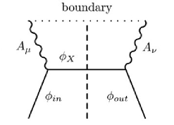
Figure 2: Witten diagram representing the $s$-channel contribution to the holographic dual description of FCS in the $N\rightarrow\infty$ limit. The vertical dashed line schematically represents the optical theorem procedure used to extract the relevant imaginary part of $T^{\mu\nu}$. There is a single-hadron intermediate state, which means that only single-hadron final states are considered in DIS. The horizontal dotted line represents the boundary of AdS₅. In addition, $\phi_{in}$, $\phi_{X}$ and $\phi_{out}$ are the dual supergravity fields of the initial, intermediate and final hadronic states, respectively, while $A_{\mu}$ couples to $J^{\mu}$ of the quantum field theory at the AdS boundary.

The sum over all possible on-shell intermediate states leads to a formula for the imaginary part of the amplitude, and allows one to obtain $F_{1}$ and $F_{2}$ and, from it, the longitudinal structure function $F_{L}$. In this case in the FCS there is only one intermediate state, which means that in the DIS that we consider there is only one outgoing single-hadron final state. Note that supergravity provides and accurate description of the holographic dual process of DIS only if $\lambda^{-1/2}\ll x<1$. This is because in this regime the Mandelstam variable $s$ (associated with the center-of-mass energy) is not large enough in order to produce excited string states. When $x$ becomes smaller than $\lambda^{-1/2}$ it is necessary to consider the full string theoretical description. On the field theory side, for $1\ll\lambda\ll N$ double-trace operators dominate the OPE. In fact two very different kinds of limits can be considered, namely, the large $N$ limit and the $q^{2}\gg\Lambda^{2}$ limit, being $\Lambda$ the IR confinement scale of the dual SYM theory.

It is very interesting to consider the case when DIS involves two-hadron states as the final states. In this case the optical theorem dictates that the holographic dual description of FCS is given in terms of one-loop Witten diagrams, which in practical terms are one-loop Feynman diagrams in type IIB supergravity. In fact, in [2] it was suggested that this process can be calculated by using supergravity. It gives the first correction to DIS in the $1/N^{2}$ expansion. Also from each supergravity Feynman diagram it is possible to extract the dependence in powers of $\Lambda^{2}/q^{2}$. It is very interesting the fact that by taking first the $N\rightarrow\infty$ limit, followed by the $q^{2}\gg\Lambda^{2}$ limit, it gives a totally different result compared with the one obtained by taking these limits the other way around. This effect has already been noted in a recent paper by Gao and Mou [16], where this question has been addressed only in part, by using an effective interaction Lagrangian in five dimensions. On the other hand, in our present work instead we start from the type IIB supergravity action in ten dimensions, including all the relevant fields, thus carrying out a first principles top-down calculation. These bulk fields correspond to specific operators of the boundary SYM theory, which in this case is an IR deformation of $SU(N)$ ${\cal{N}}=4$ SYM. In addition, we carry out the explicit calculation of all relevant $t$-channel diagrams in type IIB supergravity at leading order in $\Lambda^{2}/q^{2}$, taking into account all possible Kaluza-Klein states within the full AdS${}_{5}\times S^{5}$ solutions of the bulk fields. In comparison with our calculations, in [16] only a few Kaluza-Klein states have been considered, rendering their result incomplete in that sense. Furthermore, we obtain the explicit functional dependence on the Bjorken parameter at leading order in $\Lambda^{2}/q^{2}$. We find that this dependence is consistent with the expectations of [2] concerning the $1/N^{2}$ corrections.

Another new finding from our investigation is that it is interesting to calculate the longitudinal structure function $F_{L}=F_{2}-2xF_{1}$, extracting its explicit dependence on both $\Lambda^{2}/q^{2}$ and $1/N^{2}$, obtaining

$$F_{L} = F_{2}-2\,x\,F_{1}$$

$$= f^{(0)}_{2}\,\left(\frac{\Lambda^{2}}{q^{2}}\right)^{\Delta-1}+\frac{1}{N^{2}}\,\left(f^{(1)}_{2}-2\,x\,f^{(1)}_{1}\right)\,\left(\frac{\Lambda^{2}}{q^{2}}\right)+\frac{1}{N^{4}}\,\left(f^{(2)}_{2}-2\,x\,f^{(2)}_{1}\right)\,\left(\frac{\Lambda^{2}}{q^{2}}\right)+\cdot\cdot\cdot$$

with $\Delta\geq 4$ (where $\Delta$ is the conformal dimension associated with the incoming dilaton), in such a way that the functions $f^{(n)}_{1}$ and $f^{(n)}_{2}$ (where $n=0,1,\cdot\cdot\cdot$) give the order in $1/N^{2}$ corresponding to the expansions of $F_{1}$ and $F_{2}$, respectively. Notice that $F_{L}$ in principle contains all the terms of the form $1/N^{2n}\times\left(f^{(n)}_{2}-2\,x\,f^{(n)}_{1}\right)\,\left(\Lambda^{2}/q^{2}\right)$, which correspond to the exchange of $(n+1)$-intermediate states in the FCS, i.e. corresponding to $(n+1)$-hadron final states in DIS. From equation (1) we can observe several interesting aspects. For instance, the large $N$ limit and the limit in which $q^{2}\gg\Lambda^{2}$ do not commute, which means that at infinite $N$ the first term is the leading one, implying that the dominant contribution to DIS in this limit comes from single-hadron intermediate states in the FCS. On the other hand, if we first take the $q^{2}\gg\Lambda^{2}$ limit, the second term dominates (after considering $N\gg 1$), indicating that two-particle intermediate states give the leading contribution. Recall that this is the so-called high energy limit. Moreover, as we will show below, the rest of the contributions in this limit are subleading under certain assumptions that will be discussed later. There is an explicit tensor structure associated with each term in $F_{1}$ and $F_{2}$ in the expansion above that we will study in this work. This allows us to provide a strong argument in favor of the structure of the expansion of equation (1).

The paper is organized as follows. In the rest of this Introduction we study DIS beyond the $N\rightarrow\infty$ limit and then we briefly comment on the operator product expansion analysis of DIS at strong coupling. In sections 2 and 3 we perform the supergravity calculation of diagrams with two intermediate states in a detailed way. In Section 4 we consider some general aspects of supergravity diagrams involving multi-particle intermediate states, which imply $1/N^{2n}$ corrections to the FCS and DIS processes. In Section 5 we present the discussion and conclusions. Some details of our calculations are presented in Appendices A and B.

1.1 Two-particle intermediate states in FCS

The aim of the present work is to study the leading $1/N^{2}$ corrections to the scalar glueball structure functions in the strongly coupled regime of the gauge theory. Therefore, it is important to understand how this affects the calculation of the supergravity amplitude.

Within the AdS/CFT correspondence, the regime where classical supergravity is an accurate description of the boundary field theory is the planar limit, where the ’t Hooft coupling $\lambda=g_{YM}^{2}N$ is kept fixed and large with the condition $1\ll\lambda\ll N$. It is possible to go beyond this approximation in two directions given by two series expansions, one in powers of $1/\sqrt{\lambda}$, while the other one is the $1/N$ expansion, which for adjoint fields leads to a $1/N^{2}$ expansion. From the dual string theory point of view the strong coupling expansion ($1/\sqrt{\lambda}$) and the $1/N^{2}$ one correspond to the $\alpha^{\prime}$ expansion and the genus expansion (i.e. the string coupling $g_{s}$ expansion), respectively. In the low energy limit of type IIB superstring theory the genus expansion of type IIB string theory becomes a loop Feynman diagram expansion in type IIB supergravity, and this is the one that we study.

In the $N\rightarrow\infty$ limit only tree-level diagrams must be included. In fact, since we consider the low energy limit of type IIB superstring theory in the large $N$ limit we use type IIB supergravity at tree level. In the holographic dual calculation of DIS for scalar glueballs we are dealing with a $2\rightarrow 2$ scattering process between two gravitons and two dilatons. Therefore, in this limit we only need to study the Witten diagrams corresponding to $s$-, $t$- and $u$-channels, together with diagrams with four-point interaction vertices. In this case and also for other types of hadrons such as (holographic) mesons, it can be shown that the $s$-channel diagram is the relevant one when the center-of-mass square energy $s=-(P+q)^{2}$ is not large enough in order to produce excited string states in the holographic dual process [2, 14, 15]. However, at high energy the $t$-channel graviton exchange dominates the dynamics of the process [2, 18]. Thus, different regimes can be investigated in different ways according to the value of the Bjorken parameter: supergravity gives the full picture provided that $1/\sqrt{\lambda}\ll x<1$, however when $x\ll 1/\sqrt{\lambda}$ it is necessary to consider string theory.

Let us consider type IIB supergravity. In the Einstein frame its action is given by

$$S_{IIB}^{SUGRA}=-\frac{1}{2\kappa_{10}^{2}}\,\int d^{10}x\,\sqrt{|\det g|}\,\bigg{[}{\cal{R}}_{10}-\frac{1}{2}\,(\partial\phi)^{2}-\frac{1}{2}\,e^{2\phi}\,(\partial{\cal{C}})^{2}-\frac{1}{4\cdot 5!}\,(F_{5})^{2}\bigg{]}\,,$$ (6)

where $\phi$ is the dilaton, ${\cal{C}}$ is the Ramond-Ramond axion field and $F_{5}$ is the five-form field strength. This action must be supplemented with the self-dual condition for the five-form field strength.

An exact solution is the AdS${}_{5}\times S^{5}$ background metric

$$ds^{2}=\frac{r^{2}}{R^{2}}\,\eta_{\mu\nu}\,dx^{\mu}dx^{\nu}+\frac{R^{2}}{r^{2}}\,dr^{2}+R^{2}\,d\Omega^{2}\,,$$ (7)

where $R^{4}=4\pi g_{s}N\alpha^{\prime 2}$. In order to fix notation indices $M,N=0,1,\cdot\cdot\cdot,9$ are on AdS${}_{5}\times S^{5}$, Greek indices $\mu,\nu=0,1,\cdot\cdot\cdot,3$ and Latin indices $m,n=0,1,\cdot\cdot\cdot,4$ are on AdS₅, while Latin indices $a,b=5,6,\cdot\cdot\cdot,9$ are on $S^{5}$.

Now we describe how to perform the $1/N$-power counting in type IIB supergravity Feynman diagrams. For that we must carry out the dimensional reduction of type IIB supergravity on $S^{5}$ (see for instance [34] and also [15, 31, 32, 33]). The resulting reduced action can be written in terms of the five-dimensional dilaton $\phi_{5}(x)$ as

$$S_{5d}^{SUGRA}=-\frac{1}{2\kappa_{5}^{2}}\,\int d^{5}x\,\sqrt{|\det g_{5}|}\,\bigg{[}{\cal{R}}_{5}-\frac{1}{2}\,(\partial\phi_{5})^{2}+\dots\bigg{]}\,.$$ (8)

In this action dots indicate other terms which are not relevant in our calculation, since we only consider the $1/N^{2}$ series expansion. The constant $\kappa_{5}$ is given by

$$\frac{1}{2\kappa_{5}^{2}}=\frac{N^{2}}{8\pi^{2}R^{3}}\,.$$ (9)

Next, we define the canonically normalized fields, namely: we rescale the five-dimensional dilaton as $\tilde{\phi}_{5}\equiv N\phi_{5}$, and also we do this for the graviton. Thus, by plugging the canonically normalized fields into $S_{5d}^{SUGRA}$ we obtain the $1/N$ dependence of the three-point interaction vertices and $1/N^{2}$ dependence of the four-point ones. With them we can construct the Witten diagrams with the corresponding $1/N$-power counting.

In order to obtain the one-particle exchange contribution to the hadronic tensor and the structure functions $F_{1}$ and $F_{2}$, it is necessary to calculate the imaginary part of the amplitude associated with the $s$-channel interaction between two dilatons $\phi_{in}$ and $\phi_{out}$, and two metric perturbations (gravitons) of the form $h_{ma}=A_{m}v_{a}$. In this notation, $A_{m}$ represents a $U(1)$ gauge field in AdS₅ and $v_{a}$ is a Killing vector of the five-sphere. The only way that this can occur within type IIB supergravity is through the exchange of an intermediate dilaton $\phi_{X}$ state. The interaction action directly derived from type IIB supergravity is given by

$$S_{A\phi\phi}=\frac{1}{2\kappa_{10}^{2}}\,i{\cal{Q}}\,\int d^{10}x\,\sqrt{-g}\,A^{m}\,(\phi_{in}^{*}\,\partial_{m}\phi_{X}-\phi_{X}^{*}\,\partial_{m}\phi_{in})\,.$$ (10)

${\cal{Q}}$ is the $U(1)$ charge of the scalar field, $v^{a}\partial_{a}Y(\Omega)=i{\cal{Q}}Y(\Omega)$, where $Y(\Omega)$ represents an spherical harmonics on $S^{5}$. The corresponding five-dimensional reduced interaction action is obtained by integrating over $S^{5}$. Taking into account the dilaton rescaling and also ${\tilde{A}}_{5}^{m}\equiv NA_{5}^{m}$, it leads to

$$S^{{\tilde{A}}\tilde{\phi}\tilde{\phi}}_{5d}=\frac{1}{8\pi^{2}NR^{3}}\,i{\cal{Q}}\,\int d^{5}x\,\sqrt{|\det g_{5}|}\,{\tilde{A}}_{5}^{m}\,(\tilde{\phi}_{in,5}^{*}\,\partial_{m}\tilde{\phi}_{X,5}-\tilde{\phi}_{X,5}^{*}\,\partial_{m}\tilde{\phi}_{in,5})\,,$$ (11)

which gives a factor $1/N$ for each ${\tilde{A}}\tilde{\phi}\tilde{\phi}$ vertex. Thus, the tree-level diagram has an overall factor $1/N^{2}$, which will also be present in all the rest of loop diagrams. Since we are interested in the relative power counting between different terms in the $1/N$ expansion we will ignore the overall factor. Henceforth, we will omit the tilde on the fields.

The functional form of the non-normalizable gauge field $A_{m}$ dictates that the interaction must occur at $r_{int}\sim qR^{2}\gg r_{0}=\Lambda R^{2}$. Then, as explained, the imaginary part of the FCS amplitude is obtained by using the optical theorem, cutting the diagram in the only possible way as shown in figure 2. Thus, one has to evaluate the on-shell action $S_{A\phi\phi}$ and sum over all possible intermediate states. Note that the restriction to the $s$-channel diagram implies that the photon strikes the whole hadron, and in the case of a scalar object this leads to $F_{1}=0$. This calculation is shown schematically in figure 2 . The final result for a scalar glueball state with scaling dimension $\Delta$ has been obtained in [2] leading to

$$F_{2}(x,q^{2})=\pi\,A_{0}\,{\cal{Q}}^{2}\left(\frac{\Lambda^{2}}{q^{2}}\right)^{\Delta-1}x^{\Delta+1}(1-x)^{\Delta-2}\,,$$ (12)

where $A_{0}=2^{\Delta}\pi|c_{in}|^{2}|c_{X}|^{2}\Gamma(\Delta)^{2}$, with $c_{in}$ and $c_{X}$ being dimensionless constants.

Next, we want to calculate the first correction to these structure functions, i.e. the leading order $1/N^{2}$ contribution. This means that we have to take into account all possible type IIB supergravity one-loop corrections to the $s$-channel diagram of figure 2. In order to illustrate it, in figure 3 a few examples of the one-loop diagrams which can be constructed with the available interactions (that will be described in section 2) are shown. From the $S^{{\tilde{A}}\tilde{\phi}\tilde{\phi}}_{5d}$ action it is easy to see that since a one-loop Feynman diagram has two more vertices of the type ${\tilde{A}}\tilde{\phi}\tilde{\phi}$ (or a quartic vertex) in comparison with the tree-level Feynman diagram, then there is an additional overall factor $1/N^{2}$.

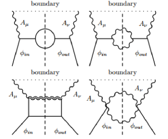
Figure 3: Some type IIB supergravity Feynman diagrams that could contribute to the one-loop correction to the FCS. Solid, wavy and double wavy lines correspond to scalar, vector and tensor perturbations from type IIB supergravity, respectively.

Notice that the cuts (vertical dashed lines) in these diagrams are only schematic: the actual computation of the imaginary part of FCS requires to square the sum of all possible supergravity Feynman diagrams having two intermediate on-shell states. Therefore, one also must consider the crossed terms. This calculation is difficult, specially in an AdS₅ background. A recent paper by Gao and Mou [16] has done a first step to attempt to address these $1/N^{2}$ corrections. However, their calculations are carried out in the context of an effective model given by a scalar-vector Lagrangian, which has a very small number of modes and interactions among them in comparison with the actual possible field fluctuations of type IIB supergravity.

In the present work we will study this problem using the full spectrum of particles and interactions from type IIB supergravity on AdS${}_{5}\times S^{5}$ and show that the $\Lambda^{2}/q^{2}\rightarrow 0$ limit renders important simplifications, leading to only one dominant diagram. The actual scattering amplitude is difficult to calculate, however our final formula will allow us to draw some conclusions about the physics of this process. We will also comment on what these observations imply on the field theory side.

1.2 Operator product expansion analysis of DIS

In this subsection we describe the OPE analysis of the DIS process in the strong coupling regime of gauge theories. We follow the analysis by Polchinski and Strassler [2], and describe it here since it will be relevant for the results of the present work. Let us consider the DIS process from the quantum field theory point of view. It is possible to perform this kind of analysis in any SYM theory like ${\cal{N}}=4$ SYM whose conformal invariance is broken by an IR cutoff $\Lambda$. The important point is to have an IR confining gauge theory. It is interesting to consider the moments of the structure functions involved in the hadronic tensor, generically defined as

$$M_{n}^{(s)}(q^{2})=\int_{0}^{1}dx\,x^{n-1}\,F^{(s)}(x,q^{2})\,.$$ (13)

These moments can be studied in terms of the OPE of two electromagnetic currents inside the hadron $J(0)\tilde{J}(q)$, whose matrix element defines the hadronic tensor. In [2] it was found that

$$M_{n}^{(s)}(q^{2})\approx \frac{1}{4}\sum_{j}C_{n,j}^{(s)}A_{n,j}\left(\frac{\Lambda^{2}}{q^{2}}\right)^{\frac{1}{2}\tau_{n,j}-1}+\frac{1}{4}\sum_{Q_{p}=Q}C_{n,p}^{(s)}A_{n,p}\left(\frac{\Lambda^{2}}{q^{2}}\right)^{\tau_{p}-1}$$

$$+\frac{1}{4N^{2}}\sum_{Q_{p}\neq Q}C_{n,p}^{(s)}a_{n,p}\left(\frac{\Lambda^{2}}{q^{2}}\right)^{\tau_{p}-1},$$

where $C^{(s)}$’s are numerical coefficients, $A$’s stand for matrix elements of the corresponding operators and $A_{n,p}=a_{n,p}N^{-2}$, while $\tau$’s account for their twist, given in terms of the conformal dimension $\Delta$, the anomalous dimension $\gamma$ and the spin $s$

$$\tau=\Delta+\gamma-s\,.$$ (15)

Equation (1.2) contains very important physical information. In the DIS regime the square momentum of the virtual photon is very large with respect to the IR confining scale $\Lambda$ , therefore the lowest twist operators dominate since their contribution are less suppressed. The first term corresponds to the contribution to the current-current OPE coming from single-trace SYM operators $T_{n,j}$. Using the normalization of the local operators in such a way that they create hadrons at order $N^{0}$, the OPE coefficients and matrix elements have the following behavior

$$C_{n,j}^{(s)} = \langle Q,P|J\,J\,T_{n,j}|Q,P\rangle\sim N^{-1}\,,$$

$$A_{n,j} = \langle Q,P|T_{n,j}|Q,P\rangle\sim N^{-1}\,.$$

The anomalous dimension of the $T_{n,j}$’s is of order $\gamma\sim\lambda^{1/4}$. Twist-two single-trace operators give the dominant contribution at weak ’t Hooft coupling. However, when the coupling becomes large this is no longer the case. The second and third terms are associated with certain double-trace operators $T_{p}^{\dagger}(\partial)^{r}T_{p}$ built from the so-called protected operators $T_{p}$. The conformal dimension of the protected operators has small or null corrections. Therefore, protected double-trace operators have the lowest twist and dominate the OPE when $\lambda$ is sufficiently large. In addition, it can be seen that among these operators there are two possibilities [2], namely:

$$A_{n,p} = \langle Q,P|T_{p}^{\dagger}(\partial)^{r}T_{p}|Q,P\rangle\sim N^{0}\,\,\,\,\textrm{if}\,\,\,\,\langle Q,P|T_{p}|0\rangle\neq 0\,,$$ (16)

$$A_{n,p} = \langle Q,P|T_{p}^{\dagger}(\partial)^{r}T_{p}|Q,P\rangle\sim N^{-2}\,\,\,\,\textrm{if}\,\,\,\,\langle Q,P|T_{p}|0\rangle=0\,.$$ (17)

The second one corresponds to the third term in equation (1.2). Obviously, at $N\rightarrow\infty$ this term is negligible and the OPE is dominated by the second term, and we can see from equation (16) that it describes a regime where hadron production is turned off. However, at finite $N$ the hadron number is not conserved, and the third term becomes important. In fact, we will see that this is the leading contribution since in this case the lower twist contributions can come from the created hadrons instead of the initial one. This is interpreted as a situation where the virtual photon strikes a pion in the hadron cloud that surrounds the incoming hadron.

On the one hand, the perturbative gauge theory analysis allows us to study the weak coupling regime. On the other hand, string theory and supergravity help us to study the strongly coupled regime. Let us focus on the case when the Bjorken parameter is within the range $0.1<x<1$, where the bulk physics can be accurately described by type IIB supergravity. Then, the process can be understood in the following way: the current operator insertion on the boundary theory generates a non-normalizable vector fluctuation of the metric (as seen in the five-dimensional reduction of type IIB supergravity) which couples with the normalizable bulk modes corresponding to hadronic states in the SYM theory. The leading behavior in the $1/N$ expansion was studied in [2] for the dilaton and the dilatino and in [14, 15] for scalar mesons and polarized vector mesons by using the optical theorem, where the leading contribution comes from a diagram with no mixing and with only one intermediate state. In this work, we build on the work started in [16] and focus on the finite $1/N^{2}$ leading contributions, by considering an external supergravity state given by a dilaton (which is the dual supergravity field of a scalar glueball state in the gauge field theory), by allowing a second intermediate state and explicitly obtain the resulting structure functions. This is equivalent to study the one-loop contribution to the supergravity interaction with two external gravi-photon states and two external dilaton states.

In principle, we would have to calculate every possible contribution coming from a Cutovsky-cut diagram allowed by type IIB supergravity, including all the Kaluza-Klein towers of modes from all the fields which develop fluctuations. Among them, for example, we can find the ones coming from the three-scalar vertex considered in [16]. This is complicated, since the geometry of AdS₅ renders Bessel function solutions, and then the integral of a generic three-particle interaction would be impossible to be carried out analytically. However, the OPE of equation (1.2) gives us an important insight into the physical process that we are trying to describe.

Reference [2] shows that when the current operator couples directly to a state of Kaluza-Klein mass $\Delta$ the resulting scattering amplitude (and the structure functions) are proportional to $\left(\Lambda^{2}/q^{2}\right)^{\Delta-1}$. This should hold regardless of the fact that this hadron might not be the initial state, since it could come from a hadron splitting into two other hadrons. This hypothesis is supported by the $1/q^{2}$-power analysis performed in [16]: by looking at the $s$-, $t$- and $u$-channel (one-loop) diagrams with scalars, we expect that the less suppressed contribution would come from the $t$-channel where the mode with the lowest Kaluza-Klein mass is exchanged (corresponding to the lowest-twist coupling). This is exactly what happens. In fact, the interaction terms present in the action imply that this is the diagram which dominates the full amplitude at strong coupling and finite $N$. The rest of diagrams are suppressed by higher powers of $1/q^{2}$. This was anticipated in reference [2].

In the rest of this paper we will obtain this particular leading amplitude and calculate the structure functions with $1/N^{2}$ corrections.

2 Supergravity calculation of diagrams with two intermediate states

2.1 The background and its $S^{5}$-reduced spectrum

The background used in this work is a deformation of type IIB supergravity on the AdS${}_{5}\times S^{5}$ of radius $R$, which can be written as

$$ds^{2}=\frac{R^{2}}{z^{2}}\left(\eta_{\mu\nu}dx^{\mu}dx^{\nu}+dz^{2}\right)+R^{2}d\Omega_{5}^{2}\,.$$ (18)

When $z=R^{2}/r$ this becomes the metric (7). In this coordinate system, the conformal boundary of the AdS space is located at $z=0$, or equivalently at $r\rightarrow\infty$ in equation (7). By introducing a cutoff $r_{0}$ it corresponds to an IR confinement scale of the boundary gauge theory $\Lambda=r_{0}/R^{2}=z_{0}^{-1}$. Recall that the self-dual five-form field strength $F_{5}$ has $N$ units of flux through the five-sphere. At low energy with respect to $1/\sqrt{\alpha^{\prime}}$ the spectrum of fluctuations of type IIB supergravity is similar to the one described in [30].

Now, let us briefly review how the full spectrum of bosonic fluctuations around the AdS${}_{5}\times S^{5}$ background is calculated. The relevant fields contained in the bosonic part of the action are the metric $G_{MN}=g_{MN}+h_{MN}$, the complex scalar $\phi$ and the RR four-form $A_{4}$ ($F_{5}=dA_{4}$ in this case). The non-zero components of $F_{5}$ with no fluctuations are

$$F_{mnopq}=\frac{1}{R}\epsilon_{mnopq}\ ,\ F_{abcde}=\frac{1}{R}\epsilon_{abcde}\,,$$ (19)

where the $\epsilon$ stands for the Levi-Civita pseudo-tensor density. Recall that the zeroth order metric $G$ and $F_{5}$ are non-vanishing. If we want to study the corresponding fluctuations we need to work out the equations of motion at quadratic order. One starts from the expansion on $S^{5}$, leading to the usual Kaluza-Klein decomposition of the fields in a basis of spherical harmonics. This includes scalar, vector and tensor (symmetric or antisymmetric) spherical harmonics that we denote as $Y^{l}(\Omega)$, $Y^{l}_{a}(\Omega)$, $Y^{l}_{(a,b)}(\Omega)$, $Y^{l}_{[a,b]}(\Omega)$, respectively. These are all eigenfunctions of the angular Laplacian $\nabla^{2}$ such that

$$\nabla^{2}Y^{l}(\Omega)=-\frac{1}{R^{2}}k(k+4)Y^{l}(\Omega)\,,$$ (20)

for some integer $k$. By separating the different components of the metric as

$$G_{mn}=g^{(AdS)}_{mn}+\tilde{h}_{mn}\,,\ \ \tilde{h}_{mn}=h_{mn}-\frac{1}{3}g_{mn}^{(AdS)}h^{a}_{\phantom{}a}\,,$$ (21)

$$G_{ma}=h_{ma}\,,\ \ G_{ab}=g_{ab}^{S^{5}}+h_{ab}\,,$$

and by fixing the De Donder-type gauge conditions $D^{a}h_{(ab)}=0$ and $D^{a}h_{am}=0$, we have

$$h_{mn}(y,\Omega)=\sum_{l}H_{mn}^{l}(y)\,Y^{l}(\Omega)\,,\ \ h_{ma}(y,\Omega)=\sum_{l}A_{m}^{l}(y)\,Y_{a}^{l}(\Omega)\,,$$

$$h_{(ab)}(y,\Omega)=\sum_{l}\phi^{l}(y)\,Y^{l}_{(ab)}(\Omega)\,,\ \ h_{\,a}^{a}(y,\Omega)=\sum_{l}\pi^{l}(y)\,Y^{l}(\Omega)\,,$$

where $y$ denotes coordinates on AdS₅ while $\Omega$ are the five angular coordinates on $S^{5}$. The expansion behaves similarly for the other fields. For instance, one important part of the $A_{4}$ fluctuations is

$$a_{mabc}(y,\Omega)=\sum_{l}a^{l}_{m}(y)\,\epsilon_{abc}^{\phantom{\alpha\beta\gamma}de}\,D_{d}\,Y_{e}^{l}(\Omega)\,.$$ (22)

This expansion simplifies considerably the linearized equations of motion. Still, some algebra is needed in order to diagonalize them, and finally a set of different Kaluza-Klein towers of particles, each one with its Kaluza-Klein mass formula, is obtained. From the combination of the metric expansion with some of the terms coming from $A_{4}$ there are three scalar particles, two vectors and one tensor. Their equations of motion, Kaluza-Klein masses and other properties are listed in table 1 . Note that the massless state of the $h_{(mn)}$ tower corresponds to the AdS₅ graviton.

Field	Spin	Build from	$m^{2}(k)$	$\Delta(k)$	${\cal{O}}_{QFT}$	$SU(4)_{R}$
$\phi$	$(0,0)$	$\phi$	$k(k+4)\,,\,k\geq 0$	$k+4$	Tr$\left(F^{2}X^{k}\right)$	$(0,k,0)$
$s$	$(0,0)$	$h^{a}_{\phantom{a}a}\ ,\ a_{abcd}$	$k(k-4)\,,\,k\geq 2$	$k$	Tr$\left(X^{k}\right)$	$(0,k,0)$
$t$	$(0,0)$	$h^{a}_{\phantom{a}a}\ ,\ a_{abcd}$	$(k+4)(k+8)\,,\,k\geq 0$	$k+8$	Tr$\left(F^{2}\tilde{F}^{2}X^{k}\right)$	$(0,k,0)$
$\Omega$	$(0,0)$	$h_{(ab)}$	$k(k+4)\,,\,k\geq 2$	$k+4$	Tr$\left(\lambda\lambda\overline{\lambda}\overline{\lambda}X^{k}\right)$	$(2,k-2,2)$
$A_{m}$	$(\frac{1}{2},\frac{1}{2})$	$h_{ma}\ ,\ a_{mabc}$	$(k-1)(k+1)\,,\,k\geq 1$	$k+3$	Tr$\left(\lambda\overline{\lambda}X^{k}\right)$	$(1,k-1,1)$
$B_{m}$	$(\frac{1}{2},\frac{1}{2})$	$h_{ma}\ ,\ a_{mabc}$	$(k+3)(k+5)\,,\,k\geq 1$	$k+7$	Tr$\left(F\tilde{F}\lambda\overline{\lambda}X^{k}\right)$	$(1,k-1,1)$
$h_{(mn)}$	$(1,1)$	$h_{(mn)}$	$k(k+4)\,,\,k\geq 0$	$k+4$	Tr$\left(F\tilde{F}X^{k}\right)$	$(0,k,0)$

Table 1: Some features of type IIB supergravity fluctuations in the AdS${}_{5}\times S^{5}$ background which are relevant to this work. The integer $k$ indicates the $SO(6)\sim SU(4)_{R}$ irrep and defines the corresponding Kaluza-Klein mass. Also, the operator that creates the boundary Fock-space state corresponding to each normalizable fluctuation is shown. The relation between the scaling dimension $\Delta$ and $k$ is shown.

We need the solutions to these equations. These are shown in Appendix A. All the normalizable bosonic modes have similar form: the modes carrying a given four-dimensional momentum $p^{\mu}$ turn out to be of the form

$$\Phi_{m_{1}\dots}\sim\epsilon_{m_{1}\dots}e^{ip\cdot x}z^{\alpha}J_{\Delta(k)-2}(pz)Y^{l(k)}(\Omega)\,$$ (23)

for some power $\alpha$ and polarization $\epsilon_{m_{1}\dots}$. The main difference between the spectrum of our confining background and the one from [30] for AdS${}_{5}\times S^{5}$ comes from the inclusion of the cutoff $z_{0}$. This imposes a restriction analogous to the one for modes in a box [2] which means that $p$ is restricted to be one of the infinite but discrete set of numbers such that $J_{\Delta(k)-2}(pz_{0})=0$ . Canonical normalization for the scalar states as defined in [1] is discussed in Appendix A.

2.2 Selection rules for the interactions

The different scalar, vector and tensor fields we studied in the previous section can interact with each other in complicated ways. These interactions can be directly obtained from the type IIB supergravity action by performing the expansion of the fields in terms of spherical harmonics on $S^{5}$. The relevant vertices will be explicitly derived in the next section. However, besides the appearance of these vertices in the action it is important to consider the selection rules coming from the fact that these particles belong to representations of the isometry group $SO(6)\sim SU(4)$. The lowest dimensional representations in which these fields are found can be viewed in [30, 36].

The selection rules can be written in terms of the Clebsh-Gordon coefficients of the tensor product decomposition in irreducible representations (irreps) of $SU(4)$ given in the notation of table 1 by

$$(0,k_{1},0)\otimes(0,k_{2},0) = \bigoplus_{i=0}^{k_{2}}\bigoplus_{j=0}^{k_{2}-i}(j,k_{1}+k_{2}-2i-2j,j)\ ,\ k_{2}\leq k_{1},$$ (24)

and similarly for the product $(0,k_{1},0)\otimes(1,k_{2},1)$. Physically, a null coefficient implies that in a scattering process where the two initial states belong to the first two irreps, a particle belonging to the third irrep cannot be among the final states. Together with the reduction of the ten-dimensional action to the five-dimensional effective one, this tells us which are the indices of the Bessel functions that can be present in the interactions when calculating the amplitudes involved in the dual DIS process. In terms of our solutions, these coefficients are given by angular integrals of combinations of the different spherical harmonics over the $S^{5}$ coordinates [37, 38]:

$$a_{123} = a(k_{1},k_{2},k_{3})=\int_{S^{5}}d\Omega_{5}\,Y^{k_{1}}Y^{k_{2}}Y^{k_{3}}\,,$$ (25)

$$b_{123} = b(k_{1},k_{2},k_{3})=\int_{S^{5}}d\Omega_{5}\,Y_{a}^{k_{3}}D^{a}Y^{k_{2}}Y^{k_{3}}\,,$$ (26)

$$c_{123} = c(k_{1},k_{2},k_{3})=\int_{S^{5}}d\Omega_{5}\,D^{a}Y^{k_{1}}D^{b}Y^{k_{2}}Y_{(ab)}^{k_{3}}\,.$$ (27)

The first integral appears when studying an interaction between scalars like $s$, $t$ or $\phi$, or tensor fields in the $(0,k_{i},0)$ representations. The second one involves two scalars and one vector. These two will appear in our calculations. The third one is written for completeness and has two scalars and one $\Omega$ field (see table 1). These factors are present in the coupling constants of the interaction vertices.

The relevant selection rules for the diagrams that we will consider are the following ones:

1. When two scalars in the $(0,k_{1},0)$ and $(0,k_{2},0)$ representations are involved in a three-particle interaction, the relevant outgoing particles can be

   • $s$, $t$, $\phi$ or $h$ particles in the $(0,k_{3}^{(1)},0)$ rep. with $|k_{1}-k_{2}|\leq k_{3}^{(1)}\leq k_{1}+k_{2}$,

   • vector particles in the $(1,k_{3}^{(2)}-1,1)$ rep. with $|k_{1}-k_{2}|+1\leq k_{3}^{(2)}\leq k_{1}+k_{2}-1$,

   • $\Omega$-scalars belonging to the $(2,k_{3}^{(3)}-2,2)$ rep. with $|k_{1}-k_{2}|+2\leq k_{3}^{(3)}\leq k_{1}+k_{2}-2$,

   where all the $k_{3}$ indices changes in two units.

2. When a scalar particle and one vector particle belong to the $(0,k_{s},0)$ and $(1,k_{v},1)$ representations interact in the same way the possible resulting particles are

   • $s$, $t$, $\phi$ or $h$ particles in the $(0,k_{3}^{(1)},0)$ rep. with $|k_{1}-k_{2}|+1\leq k_{3}^{(1)}\leq k_{1}+k_{2}-1$,

   • vector particles in the $(1,k_{3}^{(2)}-1,1)$ rep. with $|k_{1}-k_{2}|\leq k_{3}^{(2)}\leq k_{1}+k_{2}$,

   • $\Omega$-scalars in the $(2,k_{3}^{(3)}-2,2)$ rep. with $|k_{1}-k_{2}|+1\leq k_{3}^{(3)}\leq k_{1}+k_{2}-1$,

   where all the $k_{3}$ change as before.

Recall that all different integers $k$ associated with each particle are bounded from below. In fact, the existing massless particles in general correspond to the lowest representations, given by $k=1$ for vectors and $k=0$ for scalars and tensors. There is an exception given by the negative mass $s_{k=2}$ scalar. In addition, consider the case of a massless vector excitation interacting with a given scalar particle. The vector excitation can only belong to the $(1,0,1)$ representation, while the scalar one is in the $(0,k,0)$ representation for some integer $k$ associated with its dimension $\Delta$ as indicated in table 1. Then, the second selection rule implies that if we are looking for outgoing $s$, $t$ or $\phi$ scalar particles, we can only have something belonging to the same $(0,k,0)$ representation. Now, the vector representation we have chosen can only correspond to the $A_{m}$ field that represents our holographic photon, i.e. the graviton fluctuation coming from the boundary. Thus, as in the $S_{A\phi\phi}$ interaction of [2] there is no mixing for an $S_{ssA}$ vertex.

2.3 Relevant vertices

Some of the relevant interaction vertices are derived in this section. We also need the propagators of some fields, which are considered in Appendix A. Let us first focus on how the incoming dilaton can interact with two other fields. We focus on the $\phi\rightarrow s+\phi$ interaction, but other interactions may be studied in the same way. The corresponding $S_{s\phi\phi}$ vertex comes from the dilaton kinetic term

$$\int d^{10}x\sqrt{-G}\,G^{MN}\partial_{M}\phi\partial_{N}\phi\,,$$ (28)

once the mentioned fluctuations are worked out. The relevant fluctuations are given in equation (21) (and indirectly in equation (22)). The only non-vanishing modes we consider are the scalar ones plus $\tilde{h}_{(mn)}$ which cannot be completely turned off: their fluctuations are given by [36]

$$\tilde{h}^{k}_{(mn)}=D_{(m}D_{n)}\left[\frac{2}{5(k+1)(k+3)}(\pi^{k}-30b^{k})\right]\,,$$ (29)

with

$$b^{k} \equiv t^{k}-s^{k}\,,$$

$$\pi^{k} \equiv 10[(k+4)t^{k}+ks^{k}]\,.$$

Then, we have

$$\sqrt{-G}\approx\sqrt{-g}\left(1+\frac{1}{2}h^{M}_{M}\right)\,,\,\,\,G^{MN}\approx g^{MN}-h^{MN}\,,$$ (30)

where the indices are lowered and raised using the background metric $g$. By plugging these expressions into the action (28) for the case $t^{k}=0$, and integrating by parts using the Kaluza-Klein mass conditions (i.e. the equations of motion at quadratic order), it leads to

$$S_{s\phi\phi} = \frac{1}{2\kappa_{5}^{2}}\int_{AdS_{5}}dx^{5}\,\sqrt{g_{AdS_{5}}}\,a_{123}\times$$

$$\left[\frac{2k_{1}^{2}}{k_{1}+1}s_{1}D_{m}\phi_{2}D^{m}\phi_{3}-\frac{2}{k_{1}+1}D_{m}D_{n}s_{1}D^{m}\phi_{2}D^{n}\phi_{3}\right]$$

$$= \frac{1}{2\kappa_{5}^{2}}\int_{AdS_{5}}dx^{5}\,\sqrt{g_{AdS_{5}}}\,\,a_{123}\,s_{1}\phi_{2}\phi_{3}\times$$

$$\left[\frac{k_{1}^{2}}{k_{1}+1}(m_{1}^{2}-m_{2}^{2}-m_{3}^{2})+\frac{1}{2(k_{1}+1)}\left((m_{2}^{2}-m_{3}^{2})^{2}-m_{1}^{4}\right)\right].$$

Notice that $\phi_{i}$ stands for the mode with $k=k_{i}$ of $\phi$ and the corresponding Kaluza-Klein mass $m_{i}^{2}=m_{\phi}^{2}(k_{i})$. The global $N^{2}$ factor has been discussed in the introduction and is absorbed by a field redefinition, leaving canonically normalized quadratic terms, triple interactions proportional to $N^{-1}$ and quartic interactions proportional to $N^{-2}$. By writing the masses in terms of the $k_{i}$ and defining $\Sigma=\frac{1}{2}(k_{1}+k_{2}+k_{3})$ and $\alpha_{i}=\Sigma-k_{i}$ we obtain

$$S_{s\phi\phi}=\frac{1}{2\kappa_{5}^{2}}\int_{AdS_{5}}d^{5}x\,\sqrt{g_{AdS_{5}}}\,\lambda_{123}\,s_{1}\phi_{2}\phi_{3}\,,$$ (32)

where the coupling constant is given by

$$\lambda_{123}=\frac{-8\,\alpha_{3}\,\alpha_{2}(\alpha_{1}+2)(\Sigma+2)}{k_{1}+1}\,a_{123}\,.$$ (33)

The sign of the coupling is irrelevant for us since our final amplitude will be proportional to $\lambda_{123}^{2}$. However, note that $\lambda_{123}$ vanishes for $k_{1}=|k_{2}-k_{3}|$ (and also for $k_{1}=k_{2}+k_{3}+4$), which eliminates some diagrams. In fact, for $k_{1}=2$ the previous selection rules only allow $k_{3}=k_{2}-2,k_{2},k_{2}+2$, therefore we are left with the $k_{3}=k_{2}$ case. This is because there is no need to consider surface terms since all the solutions under consideration are normalizable and vanish at the boundary. Finally, when performing the integrals needed for the on-shell evaluation in the AdS₅ coordinates we use the solutions from Appendix A. First, the integration over $dx^{0}\dots dx^{3}$ implies the four-momentum conservation. Second, since the determinant behaves as $z^{-5}$ and all solutions are of the form $z^{2}J_{\Delta_{i}-2}(pz)$ we obtain a $z$-integral of the form

$$\int_{0}^{z_{0}}dz\,z\,J_{\Delta_{1}-2}(az)\,J_{\Delta_{2}-2}(bz)\,J_{\Delta_{3}-2}(cz)\,,$$ (34)

where $a,b$ and $c$ are AdS masses. Although it is difficult to solve this integral, we will analyze it in two different ways. On the one hand, the largest contribution comes from the $z\sim z_{0}$ region, which means that for numeric purposes the Bessel functions can be approximated by the asymptotic expression

$$J_{m}(z)\approx\sqrt{\frac{2}{\pi z}}\cos\left(z-\frac{m\pi}{2}-\frac{\pi}{4}\right)\,.$$ (35)

This type of numerical analysis has shown to give interesting results in our previous work [19]. On the other hand, we can have some intuition about the physics of the process from the case $z_{0}\rightarrow\infty$, where the integral is known (see Appendix B). For our purposes it is useful to approximate it by using a behavior which is easily seen from numerical integration: the result is non-zero only when one of the AdS masses is the sum of the other two .

Now, since in our diagram there are $s$ particles we need to know how they interact with the massless vector perturbation $A_{m}$ generated by the current boundary insertion. This kind of interactions has been studied before in order to obtain a more complete knowledge of the five-dimensional effective action from type IIB supergravity, and proved to be very useful to calculate $n$-point correlation functions of chiral primary operators via the AdS/CFT correspondence [35, 41, 42, 43]. The method used in these papers is slightly different from the previous one. It is based on using the equations of motion together with the self-duality condition on $F_{5}$ rather than the ten-dimensional action. The authors calculate the quadratic and cubic corrections to these equations and obtain the interaction terms present in the action leading to the corrections. Note that in this context integration by parts and surface terms appear as field redefinitions that simplify the interactions. Here, we only write the result for the triple interaction between the $A_{m}$ and two $s$ scalars [41]:

$$S_{ssA}=\frac{1}{2\kappa_{5}^{2}}\int_{AdS_{5}}d^{5}x\,\sqrt{-g}\,G_{123}A^{m}_{1}s_{2}\partial_{m}s_{3}\,,$$ (36)

where the coupling constant can be written in terms of the indices $k_{1},k_{2}$ and $k_{3}$ as

$$G_{123}=\frac{2^{5}(k_{1}+1)(\Sigma^{2}-\frac{1}{4})(\Sigma+\frac{3}{2})(\alpha_{1}-\frac{1}{2})}{(k_{1}+2)(k_{2}+1)(k_{3}+1)}\,b_{123}\,.$$ (37)

The conclusion is that $s$ modes interact with the gauge fields in a similar way as dilaton perturbations. The case $k_{2}=k_{3}=2$ will be important for us. Had we considered a complex scalar field, as we will in the next section and as was done for the dilaton in [2], we would have found exactly the same type of vertex with a gauge boson and the associated $U(1)$ current as in equation (10). Note that this interaction term must come from

$$\int d^{10}x\,\sqrt{-G}\,\left({\cal{R}}_{10}-\frac{1}{4\cdot 5!}F_{5}^{2}\right)\textrm{ plus }F_{5}=\star F_{5}\,.$$ (38)

In this case, by evaluating the vertex with the on-shell solutions and integrating it leads to the four-dimensional momentum conservation delta, now multiplied by a $z$ integral of the form

$$\int_{0}^{z0}dz\,z^{2}K_{\Delta_{1}-2}(az)J_{\Delta_{2}-2}(bz)J_{\Delta_{3}-2}(cz)\,,$$ (39)

as in the $N\rightarrow\infty$ case in [2]. We will elaborate on this in the next sub-section. Note that the Bessel function $K$ vanishes rapidly when going to the interior of AdS, which means that in this case integrating up to $z\rightarrow\infty$ is effectively the same as stopping the integration at $z_{0}$.

For completeness let us discuss another situation: the quartic vertex that would appear twice in a one-loop diagram like the fourth one in figure 3 (with gauge or scalar intermediate particles). It is obtained from the dilaton kinetic term in the action (28). We expand the determinant and the metric in terms of the fluctuations obtaining the following action in ten dimensions up to an overall constant,

$$S_{\phi\phi hh} = \int d^{10}x\sqrt{-g}\left(-\frac{1}{4}hh^{MN}\partial_{M}\phi\partial_{N}\phi+\frac{1}{8}h^{2}\partial^{P}\phi\partial_{P}\phi+\frac{1}{8}h^{M}_{N}h^{N}_{M}\partial^{P}\phi\partial_{P}\phi\right.$$ (40)

$$\ \ \ \ \ \ \ \ \ \ \ \ \ \ \ \ \ \ \ \ \ \ \ \ \ \left.+\frac{1}{2}h^{MP}h_{P}^{N}\partial_{M}\phi\partial_{N}\phi\right),$$

where $h$ denotes the trace $h^{M}_{M}$. The fields $h$ and $h_{MN}$ can be expanded in spherical harmonics and with the fluctuations of the five-form field strength, we can build for example the $s$ and $t$ scalar modes. The second term will not be considered since vector fluctuations are absent. The other terms have two dilatons coupled to $A_{m}$ and a fluctuation in the AdS₅ space. As we will see in the next section, the normalizable mode of the incident dilaton can be approximated by its asymptotic expansion near the boundary since this is where the interaction takes place. Then, the $z$-integral becomes proportional to the integral of two $J$ Bessel functions and one $K$ Bessel function. The complete integral can be calculated from equation (• ‣ B), however we are interested in the $q$-dependence

$${\cal{M}}\propto\int dz\,z^{\Delta_{1}+\alpha}K_{1}(az)J_{\Delta_{2}-2}(bz)J_{\Delta_{3}-2}(cz)K_{1}(qz)\propto a^{-\Delta_{1}}\left(\frac{b}{a}\right)^{\Delta_{2}}\left(\frac{c}{a}\right)^{\Delta_{3}}\,,$$ (41)

where $\alpha$ is a constant which depends on the normalizable solutions of the intermediate states.

Now, from dimensional analysis it is easy to see that with the normalizations used in [2] the coupling constants in triple scalar vertices with no derivatives have to be proportional to $R^{2}$. This is important in order to obtain dimensionless structure functions from the holographic FCS amplitude. In fact, final results will not depend on $R$.

In addition, we would like to note that in a general one-loop diagram one has to take into account fluctuations of all kind of fields from type IIB supergravity, including fermions. We have not discussed this here because in fact we will focus on one single diagram, and the selection rules involved in this diagram (together with consistent dimensional reduction) do not allow the appearance of these fields.

2.4 Classification of diagrams

In the previous sections we have discussed some important aspects of the particles present in the AdS${}_{5}\times S^{5}$ background with a cutoff and their possible interactions. However, we have only focused on some of them: triple interactions involving $s$ scalars, dilatons and graviton fluctuations. In this section we will see why these are all the interactions we need, and infer which diagrams must be considered in the context of the one-loop supergravity dual process of DIS.

As seen in the Introduction, the process under consideration is a $2\rightarrow 2$ scattering where both the initial and final states are two-particle states. There is a normalizable $\phi_{\Delta}$ dilaton fluctuation for some $\Delta$ and a non-normalizable massless vector field $A_{m}$ which propagates from the boundary of AdS₅ into the bulk. The dilaton is dual to the scalar glueball, while the Abelian gauge field corresponds to the virtual photon. Since the non-normalizable mode is given by a Bessel function of the form $K_{1}(qz)$ it only lives near the boundary in the small $z$ region. In the $N\rightarrow\infty$ limit particle creation is not allowed, and the incident holographic hadron has to tunnel from the interior to this region in order to interact with it, leading to a suppression of the scattering amplitude by the factor $\left(\Lambda^{2}/q^{2}\right)^{\Delta-1}$. This can be interpreted as the probability of the full hadron to shrink down to a size of order $1/q$. The details of this calculation are given in Appendix A, but the important part is that the interaction term

$$S_{A\phi\phi}=\int d^{10}x\sqrt{-G}A^{m}v^{a}\partial_{m}\phi\partial_{a}\phi\,,$$ (42)

evaluated on-shell gives an integral in the radial variable which takes the following form

$$\int_{0}^{z_{0}}dz\,z^{2}\,J_{\Delta-2}(Pz)J_{\Delta-2}(s^{1/2}z)K_{1}(qz)\approx 2^{\Delta-1}\Gamma(\Delta)\frac{q\,s^{\frac{\Delta}{2}-1}}{(s+q^{2})^{\Delta}}\,,$$ (43)

where

$$s=-(P+q)^{2}\approx-q^{2}-2P\cdot q=-\frac{q^{2}}{x}(1-x)\,,$$ (44)

is the Mandelstam variable related to the center-of-mass energy in four dimensions. The incoming momentum $P$ is not very large in comparison to $q$ or $s^{1/2}$ and we can use the asymptotic expression of $J_{\Delta-2}(z)\sim z^{\Delta-2}$ for small arguments. Thus, after squaring the result of the integral according to the optical theorem (and by considering the normalizations and the sum over intermediate states) one finds that the imaginary part of the amplitude written in terms of $q^{2}$ and $x$ has the anticipated suppression factor, and similarly for the structure functions. As explained in [2], this is exactly the suppression factor predicted by the field theory OPE as we can see from the second term in equation (1.2).

Now, the important point is that this analysis holds for any diagram where a scalar field interacts with the $A_{m}$ coming from the boundary. This is because as we have seen the vertex has the same form. Beyond the $N\rightarrow\infty$ limit, one-loop diagrams with different intermediate particles can contribute and one of these particles scatters from the interaction with the dual virtual photon. Since all the solutions have similar combinations of powers and Bessel functions, in our calculations we should find integrals like equation (43) . In consequence, we have found a hint about how each diagram will be suppressed by powers of $\Lambda^{2}/q^{2}$, and shown that it is directly related to the conformal dimension $\Delta$ of the mode that interacts with the gauge field. This is where the large $q^{2}$ limit becomes important: it classifies the different diagrams according to their relative weight in powers of $\Lambda^{2}/q^{2}$, and implies that there will be a dominant (i.e. less suppressed) contribution. This is strongly supported by the OPE formula (1.2), since the third term gives a contribution of the expected form, namely: it is suppressed by $1/N^{2}$ and with different $\Lambda^{2}/q^{2}$ powers associated with different operator twists which could be smaller than the one associated with the full target hadron. For example, the corresponding vertex of an $s$-channel diagram as in the first two cases of figure 3 will produce a suppression similar to the tree-level Witten diagram. However, when considering a diagram where the incoming dilaton splits into two particles, only one of the resulting pieces carrying some fraction of the original four-momentum interacts with the graviton perturbation near the boundary, leading to a suppression related to the nature of this particle and its Kaluza-Klein mass, defined by a conformal dimension $\Delta^{\prime}$. This is consistent with the fact that in a process like the one we are describing this intermediate particle is the only one which has to tunnel to the small-$z$ region.

Our conclusion is the following: the dominant diagram or sum of diagrams will be given by the ones where this role is played by the particle or particles with the lowest possible $\Delta^{\prime}$. This is consistent with the expectations from reference [2]. This analysis holds in more general cases as we will see in section 4. Fortunately, in the one-loop case this leads to only one possibility as the lowest $\Delta^{\prime}=2$ dimension can only be found at the bottom of the Kaluza-Klein tower corresponding to the $s$ scalar particles of table 1 . Note that this excludes for example the diagram with quartic vertices discussed in the previous section, which will always be more suppressed.

There is an interesting feature that we can discuss. The $N\rightarrow\infty$ limit leads to $F_{1}=0$ since the photon strikes the entire scalar hadron. Beyond this limit, by considering DIS with two-hadron final states it leads to a non-vanishing structure function $F_{1}$. This is due to the fact that the incoming glueball splits into two other hadrons and only one of them interacts with $A_{\mu}$ near the boundary region. Therefore, there is a set of diagrams which contribute in order that $F_{1}\neq 0$, among which there is the leading contribution.

From the detailed analysis carried out in this section and from the vertices studied in the previous subsections, we conclude that the leading diagram is the one shown in figure 4.

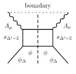
Figure 4: Witten diagram corresponding to the one-loop dominant contribution to FCS.

Although we have not written it here, we consider all the scalar solutions to have a definite charge ${\cal{Q}}_{i}$ under the $U(1)$ symmetry, and assume charge conservation in each vertex. This means that if the charge of the initial hadron is ${\cal{Q}}_{1}$, then the on-shell intermediate states must have charges ${\cal{Q}}_{2}$ and ${\cal{Q}}_{3}$, such that ${\cal{Q}}_{1}={\cal{Q}}_{2}+{\cal{Q}}_{3}$.

We ought to say that even if all the ingredients seem to support this conclusion, this is not a full proof. This is hard to do since the definite integrals with three or four Bessel functions arising from the evaluation of the amplitude and in particular from integrations in $z$ are not known analytically in every parametric regime (for the AdS masses) and for any combination of indices. However, this analysis should be extensive to other theories whose dual backgrounds are asymptotic to AdS${}_{5}\times S^{5}$. In fact, for any asymptotically AdS${}_{5}\times C^{5}$ background, where $C^{5}$ stands for some compact five-dimensional Einstein manifold, the idea would be the same: to find the excitation with the smallest conformal dimension and construct the diagram or diagrams where the initial hadron produces this particle, which is the one that interacts with the holographic virtual photon.

3 Results for the structure functions

3.1 General considerations and tensor structure

Once the leading diagram and the relevant interaction terms are identified, we work out an expression for the imaginary part of the scattering amplitude and extract the order $1/N^{2}$ contributions to the hadronic tensor and its structure functions. The imaginary part of $T^{\mu\nu}$ is obtained by using the optical theorem. We must calculate the scattering amplitude for the process at the left-hand side of the vertical cut of figure 4 with on-shell outgoing particles, and then square the resulting amplitude and sum over all possible intermediate states. In comparison with the $N\rightarrow\infty$ case, there is now an off-shell state: the propagating $s$ scalar represented in this figure by a vertical line on each side of the cut. This state is very important, since as we have seen its conformal dimension $\Delta^{\prime}=2$ ensures that we obtain the smallest $\Lambda^{2}/q^{2}$ suppression.

This is also depicted in figure 5, where we define the momenta and mass notation which we use in the rest of the paper.

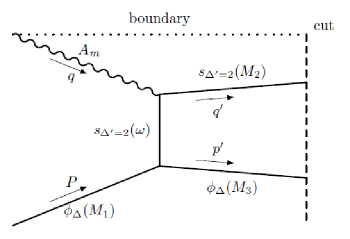
Figure 5: Feynman diagram corresponding to the left-hand side of the cut. The field associated with each line is explicitly presented along with the notation for the four-dimensional momenta, conformal dimensions and AdS masses. The solutions are described in Appendix A.

Notice that we use $q^{\prime 0}=\sqrt{M_{2}^{2}+|\vec{q^{\prime}}|^{2}}$ and $p^{\prime 0}=\sqrt{M_{3}^{2}+|\vec{p^{\prime}}|^{2}}$. We will work in the center-of-mass frame, where

$$P^{0}=|\vec{P}|=|\vec{q}|=\frac{q}{2\sqrt{x(1-x)}},\ |\vec{q^{\prime}}|=|\vec{p^{\prime}}|\textrm{ and }q^{0}=\frac{(1-2x)q}{2\sqrt{x(1-x)}}\,.$$ (45)

Now, let us define the following vectors as

$$v_{s}^{\mu}=\frac{1}{q}\left(P^{\mu}+\frac{q^{\mu}}{2x}\right)\ \textrm{and}\ v_{t}^{\mu}=\frac{1}{q}\left(q^{\prime\mu}+\frac{q^{\mu}}{2y^{\prime}}\right)\ \textrm{with}\ y^{\prime}=\frac{-q^{2}}{2q^{\prime}\cdot q}\,.$$ (46)

The auxiliary variable $y^{\prime}$ can be thought of as equivalent to the Bjorken parameter $x$ for the scattering of the $s$ scalar and the gauge field.

In the field theory side, this will lead to the dominant contribution of the $W^{\mu\nu}$ hadronic tensor for interactions with two intermediate states $X_{1}$ and $X_{2}$, and we can schematically write

$$\textrm{Im}\left(T_{2}^{\mu\nu}\right) = \pi\sum_{X_{1},X_{2}}\langle P,Q|\tilde{J}^{\mu}(q)|X_{1},X_{2}\rangle\langle X_{1},X_{2}|J^{\nu}(0)|P,Q\rangle$$

$$= \pi\sum_{M_{2},M_{3}}\int\frac{d^{3}p^{\prime}}{2E_{p^{\prime}}(2\pi)^{3}}\frac{d^{3}q^{\prime}}{2E_{q^{\prime}}(2\pi)^{3}}\langle P,Q|\tilde{J}^{\mu}(q)|X_{1},X_{2}\rangle\langle X_{1},X_{2}|J^{\nu}(0)|P,Q\rangle$$

$$= 4\pi^{3}\sum_{M_{2},M_{3}}\int\frac{d^{4}q^{\prime}}{(2\pi)^{4}}\delta\left(M_{2}^{2}-q^{\prime 2}\right)\delta\left(M_{3}^{2}-(P+q-q^{\prime})^{2}\right)|\langle P,Q|J^{\nu}(0)|X_{1},X_{2}\rangle|^{2},$$

where the subindex in $T^{\mu\nu}_{2}$ indicates that we are considering only processes with two-particle intermediate states, and

$$n_{\mu}\langle P,Q|\tilde{J}^{\mu}(q)|X_{1},X_{2}\rangle=(2\pi)^{4}\delta^{4}\left(P+q-p^{\prime}-q^{\prime}\right)\langle P,Q|n\cdot J(0)|X_{1},X_{2}\rangle\,,$$ (48)

is identified in the AdS/CFT context with what we have been calling the amplitude on each side of the cut. Thus, we obtain the following hadronic tensor

$$W_{2}^{\mu\nu}=\sum_{M_{2},M_{3}}c^{2}\int\frac{d^{3}p^{\prime}}{2E_{p^{\prime}}(2\pi)^{3}}\frac{d^{3}p^{\prime}}{2E_{p^{\prime}}(2\pi)^{3}}(2\pi)^{4}\delta^{4}\left(P+q-p^{\prime}-q^{\prime}\right)v_{t}^{\mu}v_{t}^{\nu}|C_{t}|^{2}\,,$$ (49)

where $c^{2}\equiv c_{1}^{2}c_{2}^{2}c_{3}^{2}$ stands for square of the product of the normalization constants of each on-shell field. The complex scalar factor $C_{t}$ contains all the information from the evaluation of the vertices and the propagator of the diagram as well as from the AdS₅ solutions, with the exception of the phase factors and the integrals on the $x^{\mu}$ coordinates which only give the four-momentum conservation. By plugging the explicit solutions and the propagator given in Appendix A, equation (95), we can schematically write

$$C_{t}(M_{2},M_{3},p^{\prime},q^{\prime})=\int dz\,dz^{\prime}\left[V_{ssA}(z)\times V_{s\phi\phi}(z^{\prime})\times G(z,z^{\prime})\right]\,,$$ (50)

where we omit the integration of the spherical harmonics on the $S^{5}$ whose contribution was explained in the previous sections.

Then, from the $v_{t}^{\mu}v_{t}^{\nu}$ factor of this holographic hadronic tensor, which is consequence of that the $t$-channel diagram gives the leading contribution, it is easy to separate the $1/N^{2}$ contributions to each structure function. This is because from equation (4) we know that

$$\left(\eta_{\mu\nu}-\frac{q_{\mu}q_{\nu}}{q^{2}}\right)W^{\mu\nu} = \eta_{\mu\nu}W^{\mu\nu}=3q^{2}F_{1}+2xv_{s}^{2}F_{2}\,,$$ (51)

$$q^{2}(v_{s})_{\mu}(v_{s})_{\nu}W^{\mu\nu} = P_{\mu}P_{\nu}W^{\mu\nu}=q^{2}v_{s}^{2}F_{1}+2xv_{s}^{4}F_{2}\,.$$ (52)

Thus, we obtain

$$F_{1}(x,q^{2}) = \sum_{M_{2},M_{3}}c^{2}\int\frac{d^{3}p^{\prime}}{2E_{p^{\prime}}(2\pi)^{3}}\frac{d^{3}p^{\prime}}{2E_{p^{\prime}}(2\pi)^{3}}(2\pi)^{4}\delta^{4}\left(P+q-p^{\prime}-q^{\prime}\right)|C_{t}|^{2}$$ (53)

$$\,\,\,\,\,\,\,\,\,\,\,\,\,\,\,\,\,\,\,\,\,\,\,\,\,\,\,\,\times 2q^{2}\left[v_{t}^{2}+4x^{2}(v_{s}\cdot v_{t})^{2}\right],$$

$$F_{2}(x,q^{2}) = \sum_{M_{2},M_{3}}c^{2}\int\frac{d^{3}p^{\prime}}{2E_{p^{\prime}}(2\pi)^{3}}\frac{d^{3}p^{\prime}}{2E_{p^{\prime}}(2\pi)^{3}}(2\pi)^{4}\delta^{4}\left(P+q-p^{\prime}-q^{\prime}\right)|C_{t}|^{2}$$ (54)

$$\,\,\,\,\,\,\,\,\,\,\,\,\,\,\,\,\,\,\,\,\,\,\,\,\,\,\,\,\times 4xq^{2}\left[v_{t}^{2}+12x^{2}(v_{s}\cdot v_{t})^{2}\right]\,.$$

As we will see in the next section this decomposition holds in a more general situation. Before obtaining $|C_{t}|^{2}$ we can already see that the first two terms which contribute to the structure functions $F_{1}$ and $F_{2}$ can be thought of as related by the Callan-Gross relation

$$F^{*}_{2}(x,q^{2})=2\,x\,F^{*}_{1}(x,q^{2})\,,$$ (55)

where the star means that these are not the complete structure functions but only the first term between brackets in the corresponding leading $1/N^{2}$ contribution. In contrast, the second terms in $F_{1}$ and $F_{2}$ give non-zero contributions to the longitudinal structure function

$$F_{L}=F_{2}-2\,x\,F_{1}\,.$$ (56)

This will be important when analyzing our results in terms of the internal structure of the hadron. We will discuss more about this in Section 5.

3.2 Details of the amplitude computation

Now, let us consider some details of the calculation of the structure functions, i.e. the computation of (53) and (54).

There are different parts of the calculation that we have to assembly. First, we discuss the terms that are common to both structure functions: the momenta integrations, the sum over intermediate states and the complex scalar $C_{t}$ with the contribution of both vertices. Then, we will write the dimensionless factors, which define each structure function in terms of the relevant kinematic parameters. Note that at the end all $R$ factors cancel, thus we will omit them.

• There is an integral over the space component of the momenta $\vec{p^{\prime}}$ and $\vec{q^{\prime}}$, as well as a factor associated with the energy-momentum conservation. This can be easily rewritten in the center-of-mass frame and by using spherical coordinates, where all the integrals but one can be solved trivially. The remaining one is an angular integral in the variable $\theta$, the angle between the incoming and outgoing vector momenta $q$ and $q^{\prime}$,

  $$\int\frac{d^{3}q^{\prime}}{(2\pi)^{3}2E_{q^{\prime}}}\int\frac{d^{3}p^{\prime}}{(2\pi)^{3}2E_{p^{\prime}}}(2\pi)^{4}\delta^{(4)}(P+q-p^{\prime}-q^{\prime})(\dots)=\frac{|\vec{p^{\prime}}|}{8\pi q}\sqrt{\frac{x}{1-x}}\int d\theta\sin\theta(\dots)$$

  where $|\vec{p^{\prime}}|$ solves the algebraic equation

  $$q\sqrt{\frac{1-x}{x}}=\sqrt{|\vec{p^{\prime}}|^{2}+M_{2}^{2}}+\sqrt{|\vec{p^{\prime}}|^{2}+M_{3}^{2}}\,.$$ (57)

• There is a factor $c^{2}$ corresponding to the product of the normalizations of all states involved in the process given by $c_{1}^{2}c_{2}^{2}c_{3}^{2}$. If we assume that the masses are known this is easy to compute since in all cases the normalization integral is dominated by the region $z\sim z_{0}=\Lambda^{-1}$. The arguments of the Bessel functions cannot be small, therefore we can use the asymptotic expression (35). In this way an on-shell scalar field solution associated with this Bessel function $J_{\Delta-2}$ comes with a normalization constant $c_{\Delta}$ such that

  $$c_{\Delta}^{2}=\left(\frac{\sqrt{2}}{z_{0}|J_{\Delta-1}(kz_{0})|}\right)^{2}\sim\frac{kz_{0}}{z_{0}^{2}}=k\Lambda\,,$$ (58)

  up to numerical factors. In the last step we have used the fact that since $kz_{0}$ is a zero of $J_{\Delta-2}$, it must be either a minimum or a maximum of $J_{\Delta-1}$ because of the recursion relations for the derivative of these functions.

• There is a sum over the masses of the intermediate on-shell states, $M_{2}$ and $M_{3}$. The masses are constrained by the energy conservation (57). Thus, we have

  $$\sum_{M_{2}M_{3}}\equiv\sum_{M_{2}=0}^{q\sqrt{\frac{1-x}{x}}}\sum_{M_{3}=0}^{q\sqrt{\frac{1-x}{x}}-M_{2}}.$$ (59)

The complex scalar $C_{t}$ contains the information of the vertices and the propagator (95), including the coupling constants $\lambda_{123}$ and $G_{123}$ with the corresponding $k$ indices. In what follows we will collect these in a dimensionless constant $B$ independent of $q^{2}$ and $x$ whose exact form is irrelevant for our conclusions. We can take the $\omega$-integral out in order to factorize the other integrals, obtaining

$$C_{t}=q\int d\omega\,\frac{\omega}{\omega^{2}+(P-p^{\prime})^{2}}\,S^{(z)}_{ssA}(M_{2},q,\omega)\,S^{(z^{\prime})}_{s\phi\phi}(M_{1},M_{3}\,,\omega)\,,$$ (60)

where $S^{(z)}_{ssA}$ and $S^{(z^{\prime})}_{\phi\phi s}$ are integrals over $z$ and $z^{\prime}$, respectively. We will explain briefly each term and calculate the integral below. Thus, we have:

• An integral (or sum) in the variable $\omega$ of the intermediate field $s$ and its propagator given by

  $$\frac{\omega}{\omega^{2}+(P-p^{\prime})^{2}}=\frac{\omega}{\omega^{2}-M_{1}^{2}-M_{3}^{2}+\frac{q}{\sqrt{x(1-x)}}\left(\sqrt{|\vec{p^{\prime}}|^{2}+M_{3}^{2}}-|\vec{p^{\prime}}|\cos\theta\right)}\,.$$ (61)

• An integral associated with the interaction between the three scalar modes (two dilatons and the scalar $s$)

  $$S^{(z^{\prime})}_{s\phi\phi}=\int_{0}^{z_{0}}dz^{\prime}z^{\prime 2}\,J_{\Delta-2}(M_{1}z^{\prime})J_{0}(\omega z^{\prime})J_{\Delta^{\prime\prime}-2}(M_{3}z^{\prime})\,,$$ (62)

  where $\Delta$ labels the spherical harmonics corresponding to the initial dilaton, while $\Delta^{\prime\prime}$ is associated with the intermediate dilaton field which has mass $M_{3}$. The leading contribution to this integral is given by the region $z\sim z_{0}\gg 1$. Thus, we can approximate the Bessel functions for large arguments. By considering both approximations of the integrals and numerical integration one finds that this integral behaves as (111)

  $$S^{(z^{\prime})}_{s\phi\phi}\sim\frac{1}{\sqrt{M_{1}M_{3}}}\left[\delta(\omega-|M_{1}-M_{3}|)\pm\delta(\omega-(M_{1}+M_{3}))\right]\,,$$ (63)

  where the dependence on $\Delta$ and $\Delta^{\prime\prime}$ is only reflected on the $\pm$ signs in front of each term (see Appendix B). This will allow us to perform the integral in $\omega$.

• An integral associated with the interaction vertex between two fields $s$ and the non-normalizable vector perturbation $A_{\mu}$. By using the axial gauge the corresponding $z$-integral becomes

  $$S^{(z)}_{ssA}=\int_{0}^{z_{0}}dzz^{2}\,K_{1}(qz)J_{0}(\omega z)J_{0}(M_{2}z)\,,$$ (64)

  where the Bessel function $K_{1}(qz)$ quickly decreases in the bulk which allows one to approximate the upper limit by $z\rightarrow+\infty$. We can solve the integral using the equation (• ‣ B) with $\rho=3$, $\lambda=0$, $\mu=0$ and $\nu=1$ from the appendix. For $\omega<<q$ the expression for the Bessel function $J_{0}(\omega z)$ at small arguments can be used, and this corresponds to consider $J_{0}(\omega z)\sim 1$. Therefore from equation (114), we obtain

  $$S^{(z)}_{ssA}=\frac{2q}{\left(M_{2}^{2}+q^{2}\right)^{2}}\,.$$ (65)

  Notice that both for $M_{2}<<1$ and $M_{2}\sim q$ this provides an order $q^{-3}$ factor.

Recall that the factors which appear in the last three items enter the definition of $C_{t}$, and therefore they must be squared in order to give $|C_{t}|^{2}$ before doing the angular integral.

Finally, we have the dimensionless factor which define the structure function,

$$\left(\begin{array}[]{c l}F_{1}\\ F_{2}\\ F_{L}\end{array}\right)=\frac{1}{N^{2}}\sum_{M_{1}M_{2}}c^{2}\frac{q|\vec{p^{\prime}}|}{8\pi}\sqrt{\frac{x}{1-x}}\int d\theta\sin\theta\left(\begin{array}[]{c l}v_{t}^{2}+4x^{2}(v_{s}\cdot v_{t})^{2}\\ 2x[v_{t}^{2}+12x^{2}(v_{s}\cdot v_{t})^{2}]\\ 16x^{3}(v_{s}\cdot v_{t})^{2}\end{array}\right)|C_{t}|^{2}\,.$$ (66)

Henceforth, the prefactor $1/N^{2}$ carries all the $N$-dependence of the structure functions coming from the rescaled fields. Without any approximation the dimensionless factors in the parenthesis can be written in terms of $M_{2}$, $M_{3}$ and $\theta$ as,

$$\frac{|\vec{p^{\prime}}|^{2}}{q^{2}}\left[1-\cos^{2}\theta\right]\,,\ \ \frac{1}{(1-x)q^{2}}\left[\left(q^{\prime 0}+(2x-1)|\vec{p^{\prime}}|\cos\theta\right)^{2}\right]\,,$$

$$\textnormal{and}\ \ \ \frac{1}{(1-x)q^{2}}\left[2x(1-x)|\vec{p^{\prime}}|^{2}\left(1-\cos^{2}\theta\right)+\left(q^{\prime 0}+(2x-1)|\vec{p^{\prime}}|\cos\theta\right)^{2}\right]\,,$$ (67)

for $F_{1}$, $F_{L}$ and $F_{2}$ respectively.

These are all the ingredients needed for the calculation of the structure functions.

3.3 Angular integral and final results for the structure functions

Among the previous discussion the most difficult part of the calculation is the angular integral. Recall that the factor which depends on the angle $\theta$ is $|C_{t}|^{2}$ (through $(P-p^{\prime})^{2}$ in the denominator of the propagator) multiplied by the combination of $v_{t}^{2}$ and $(v_{s}\cdot v_{t})^{2}$ for each of the structure functions.

The longitudinal structure function $F_{L}$, on which we will focus, takes the following expression,

$$F_{L} = \frac{1}{N^{2}}B^{2}\sum_{M_{2},M_{3}}\Lambda^{3}M_{1}M_{2}M_{3}\int d\theta\sin(\theta)\frac{1}{8\pi}\sqrt{\frac{x}{1-x}}|\vec{p^{\prime}}|q^{3}\left[\frac{\left(q^{\prime 0}+(2x-1)|\vec{p^{\prime}}|\cos(\theta)\right)^{2}}{(1-x)q^{2}}\right]$$ (68)

$$\times\left(\int d\omega\frac{\omega}{\omega^{2}+\left(P-p^{\prime}\right)^{2}-i\epsilon}S^{(z^{\prime})}_{s\phi\phi}(\omega,M_{1},M_{3})S^{(z)}_{ssA}(\omega,q,M_{2})\right)^{2}.$$

By using equation (63) the integral becomes

$$F_{L}=\frac{1}{N^{2}}B^{2}\sum_{M_{2},M_{3}}\Lambda^{3}M_{2}\int d\theta\sin(\theta)\frac{1}{8\pi}\sqrt{\frac{x}{1-x}}|\vec{p^{\prime}}|q^{3}\left[\frac{\left(q^{\prime 0}+(2x-1)|\vec{p^{\prime}}|\cos(\theta)\right)^{2}}{(1-x)q^{2}}\right]\times$$

$$\left(\int d\omega\frac{\omega}{\omega^{2}+\left(P-p^{\prime}\right)^{2}-i\epsilon}\left[\delta(\omega-|M_{1}-M_{3}|)\pm\delta(\omega-(M_{1}+M_{3}))\right]S^{(z)}_{Ass}(\omega,q,M_{2})\right)^{2}.$$

Let us consider the case $M_{3}\ll q$ and $|\vec{p^{\prime}}|\sim q$ which leads to the leading contribution . The conditions over the mass $M_{1}\ll q$ implies that $\omega=|M_{1}\pm M_{3}|\ll q$ allowing one to solve approximately the integral $S^{(z)}_{ssA}(|M_{1}\pm M_{3}|,q,M_{2})$ from equation (65). In order to solve the integral in $\theta$ we can expand the denominator in the propagator considering $M_{3}\ll|\vec{p^{\prime}}|$. This restriction imposes a condition on the upper limit of $M_{2}$ in the sum, since for $M_{2}$ close to the maximum we can see from the definition (57) that $|\vec{p^{\prime}}|$ should be small or vanishing. By expanding $p^{0}$ and $p^{\prime 0}$, we obtain

$$p^{\prime 0}=\sqrt{|\vec{p^{\prime}}|^{2}+M_{3}^{2}}\approx|\vec{p^{\prime}}|+\frac{M_{3}^{2}}{2|\vec{p^{\prime}}|}-\frac{M_{3}^{4}}{8|\vec{p^{\prime}}|^{3}}\,,$$ (70)

$$p^{0}=\sqrt{|\vec{p}|^{2}+M_{1}^{2}}\approx|\vec{p^{\prime}}|+\frac{M_{1}^{2}}{2|\vec{p}|}-\frac{M_{1}^{4}}{8|\vec{p}|^{3}}\,.$$ (71)

Thus, the denominator becomes

$$(M_{1}\pm M_{3})^{2}+(P-p^{\prime})^{2}\approx 2|\vec{p}||\vec{p^{\prime}}|\left(1-\cos(\theta)\right)+\frac{|\vec{p}|}{|\vec{p^{\prime}}|}\left(M_{3}\pm M_{1}\frac{|\vec{p^{\prime}}|}{|\vec{p}|}\right)^{2}+{\cal{O}}(M_{1}^{4})\,.$$ (72)

The largest contribution comes from the small $\theta$ region in the term with a minus sign. This is so because for $\theta=0$, $M_{3}=\alpha M_{1}$ with $\alpha=|\vec{p^{\prime}}|/|\vec{p}|$ is a zero of the denominator. Therefore, we will focus on the term with the minus sign. The possible divergence will be addressed later. Notice that the expression above contains two Dirac deltas, but the term we will focus on has a very simple physical interpretation: for $M_{3}<M_{1}$ and $M_{3}+\omega=M_{1}$ it represents a process in which the incoming hadron splits into two hadrons, each one carrying a fraction of the incident four-momentum.

The condition $M_{3}\ll|\vec{p^{\prime}}|$ implies that the dimensionless factor of $F_{L}$ is approximately

$$\left[\frac{\left(q^{\prime 0}+(2x-1)|\vec{p^{\prime}}|\cos\theta)\right)^{2}}{(1-x)q^{2}}\right]\approx\frac{1}{x}\left[1+\sqrt{\frac{x}{1-x}}\frac{|\vec{p^{\prime}}|}{q}\left((2x-1)\cos\theta-1\right)\right]^{2}\,.$$ (73)

Under the mentioned approximations we obtain

$$F_{L}=\frac{1}{N^{2}}B^{2}\sum_{M_{2},M_{3}}\frac{\Lambda^{3}M_{2}q^{5}}{(M_{2}^{2}+q^{2})^{2}}\frac{|\vec{p^{\prime}}|}{2\pi}\frac{(M_{1}-M_{3})^{2}}{\sqrt{x(1-x)}}$$

$$\times\int_{0}^{\pi}\frac{d\theta\sin(\theta)\left[1+\sqrt{\frac{x}{1-x}}\frac{|\vec{p^{\prime}}|}{q}\left((2x-1)\cos\theta-1\right)\right]^{2}}{\left[2|\vec{p}||\vec{p^{\prime}}|(1-\cos\theta)+\frac{|\vec{p}|}{|\vec{p^{\prime}}|}(M_{3}-M_{1}\alpha)^{2}\right]^{2}}\,.$$ (74)

The integral in $\theta$ now can be solved, and by considering the $1/q^{2}$ expansion we obtain

$$\int_{0}^{\pi}d\theta\frac{\sin(\theta)\left[1+\sqrt{\frac{x}{1-x}}\frac{|\vec{p^{\prime}}|}{q}\left((2x-1)\cos\theta-1\right)\right]^{2}}{\left[2|\vec{p}||\vec{p^{\prime}}|(1-\cos\theta)+\frac{|\vec{p}|}{|\vec{p^{\prime}}|}(M_{3}-M_{1}\alpha)^{2}\right]^{2}}=\frac{\left(1-2\sqrt{x(1-x)}\frac{|\vec{p^{\prime}}|}{q}\right)^{2}}{2|\vec{p}|^{2}(M_{3}-M_{1}\alpha)^{2}}+{\cal{O}}\left(\frac{\log q}{q^{4}}\right)\,.$$ (75)

Then,

$$F_{L}=\frac{1}{N^{2}}\sum_{M_{2}}\frac{\Lambda^{3}M_{2}q^{5}}{(M_{2}^{2}+q^{2})^{4}}\frac{|\vec{p^{\prime}}|}{2\pi}\frac{\left(1-2\sqrt{x(1-x)}\frac{|\vec{p^{\prime}}|}{q}\right)^{2}}{2|\vec{p}|^{2}\sqrt{x(1-x)}}\sum_{M_{3}}\frac{(M_{1}-M_{3})^{2}}{(M_{3}-M_{1}\alpha)^{2}}\,.$$ (76)

From the sum over $M_{3}$ we keep the most important contribution, given by the term where $M_{3}$ is as close as possible to $\alpha M_{1}$. Recall that $M_{3}$ can only take a few discrete values due to the presence of the cutoff $\Lambda$. Then, we assume a representative value $M_{3}=\alpha M_{1}+\Lambda$. Thus, we take

$$\sum_{M_{3}}\frac{(M_{1}-M_{3})^{2}}{(M_{3}-M_{1}\alpha)^{2}}\approx\frac{M_{1}^{2}(\alpha-1)^{2}}{\Lambda^{2}}\,.$$ (77)

This term depends on $\alpha=\frac{|\vec{p^{\prime}}|}{|\vec{p}|}$, which implicitly depends on $M_{2}$ through the definition of $|\vec{p^{\prime}}|$.

Then, we approximate the sum over $M_{2}$ by an integral, similarly to what is done for $M_{X}$ in [2]. The upper limit is given by a fraction $0<c<1$ of the center-of-mass energy $q\sqrt{\frac{1-x}{x}}$. Notice that $c$ should be restricted by the condition $|\vec{p^{\prime}}|\gg M_{3}$. Then, $|\vec{p^{\prime}}|$ can be written as a function of $M_{2}$ and $q$ from the equation

$$|\vec{p^{\prime}}|\approx\frac{q}{2}\sqrt{\frac{1-x}{x}}-\frac{M_{2}^{2}}{2q}\sqrt{\frac{x}{1-x}}\,.$$ (78)

Therefore, we find

$$F_{L} = \frac{M_{1}^{2}}{N^{2}}B^{2}\Lambda\int_{0}^{cq\sqrt{\frac{1-x}{x}}}\frac{dM_{2}}{\Lambda}\frac{M_{2}q^{4}}{(M_{2}^{2}+q^{2})^{4}}\left(1-x\left(1+\left(\frac{M_{2}}{q}\right)^{2}\right)\right)x^{4}\left(1+\left(\frac{M_{1}}{q}\right)^{2}\right)^{4}$$ (79)

$$= \frac{1}{N^{2}}B^{2}c^{2}(2-c^{2})\frac{M_{1}^{2}}{4\pi q^{2}}x^{3}(x-1)^{2}\,,$$

where $B$ is a dimensionless constant that contains the corresponding coupling constants $\lambda_{123}$ and $G_{123}$ of Section 2.3 with the $k$ indices corresponding to each particle. We can see that $F_{L}$ has a maximum around $x\approx 0.6$ and vanishes for $x=1$ as expected. Note that the $x$-dependence of this result is independent of the value of $c$. Also, recall that the solutions are such that the AdS masses (as $M_{1}$) are proportional to $\Lambda$.

For $F_{1}$ the integrals in $z$, $z^{\prime}$ and $\omega$ can be solved in a similar way as for $F_{L}$. The main difference comes from the dimensionless factor in the angular integral. We obtain

$$F_{1} = \frac{1}{N^{2}}\sum_{M_{2},M_{3}}\Lambda^{3}\frac{M_{2}q^{5}}{(M_{2}^{2}+q^{2})^{4}}\frac{1}{8\pi}\frac{(M_{1}-M_{3})^{2}\sqrt{x}}{\sqrt{(1-x)}}|\vec{p}^{\prime}|$$

$$\times\int_{0}^{\pi}d\theta\sin(\theta)\frac{\frac{|\vec{p}^{\prime}|^{2}}{q^{2}}(1-\cos^{2}\theta)}{\left[2|\vec{p}||\vec{p}^{\prime}|(1-\cos\theta)+\frac{|\vec{p}|}{|\vec{p}^{\prime}|}(M_{3}-M_{1}\alpha)^{2}\right]^{2}}\,.$$

The integrals over $M_{2}$ and $M_{3}$ are very complex and we can not obtain an analytic result for $F_{1}$. However, if we estimate the $q$-power counting, it turns out that the structure function $F_{1}$ has a $\frac{\log q}{q^{4}}$ dependence. Therefore, $F_{1}$ is non-vanishing but subleading.

4 Multi-particle intermediate states from type IIB supergravity

In this section we study the situation where there are multi-particle intermediate states in the FCS. We investigate this by considering Witten diagrams with multi-particle intermediate states from type IIB supergravity. The idea is to show that both the tensor structure (and the decomposition of the scattering amplitude in structure functions) and the $\Lambda^{2}/q^{2}$ dependence are the same for any number of loops from the supergravity point of view. We also give arguments to motivate the following conjecture: within the supergravity regime, all the $n$-loop with $n\geq 1$ leading contributions to DIS are suppressed by the same power of $\Lambda^{2}/q^{2}$ than the $n=1$ case that we have studied in detail in this work. We only consider Witten diagrams such that an scalar $s$ with the smaller scaling dimension $\Delta^{\prime}=2$ interacts with the non-normalizable gauge field. We assume the separation of this interaction region from the rest of the multi-particle exchange process, which occurs in the IR. This is because if the first masses are small, all the others are bounded to be of the same order due to the form of the vertices present in the splitting of the original hadron, which involve normalizable modes and render a $z$-integral of the type of our $s\phi\phi$ interaction. This type of diagrams give the most relevant contribution for the reasons explained in the previous sections. Figure 6 schematically represents this kind of diagrams.

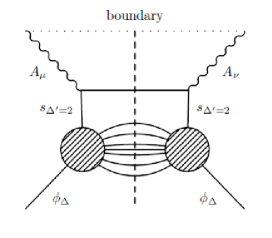
Figure 6: Relevant Witten diagrams at a generic loop-level.

We can start from the most general Lorentz-tensor decomposition of the hadronic tensor

$$W^{\mu\nu}=F_{1}(x,q^{2})\left(\eta^{\mu\nu}-\frac{q^{\mu}q^{\nu}}{q^{2}}\right)+F_{2}(x,q^{2})2\,x\,v_{s}^{\mu}\,v_{s}^{\nu}\,,$$ (80)

and the solution of the $U(1)$ gauge field which is a perturbation of the bulk metric, induced by the current operator inserted in the AdS boundary given by

$$A_{\mu}(x,z)=e^{iq\cdot x}\left[c_{\mu}qzK_{1}(qz)+\frac{n\cdot q}{q^{2}}q_{\mu}\right]\ ,\ c_{\mu}=n_{\mu}-\frac{n\cdot q}{q^{2}}q_{\mu}\ ,\ A^{\mu}=z^{2}\eta^{\mu\nu}A_{\nu}.$$ (81)

This solution has been obtained within the axial gauge, for which $A_{z}=0$, using the boundary condition

$$A_{\mu}(x,z\rightarrow 0)=n_{\mu}e^{iq\cdot x}\,.$$ (82)

The tensor structure of the amplitude is

$$\textrm{Im}({\cal{A}})\sim n_{\mu}n_{\nu}\textrm{Im}(T^{\mu\nu})\,.$$ (83)

The relevant interaction is the one on the vertex closer to the boundary, given by $S_{ssA}$ or $S_{A\phi\phi}$, which appears in all the Witten diagrams we are considering. Using the dilaton field solutions in the axial gauge (see Appendix A) $\phi$, this vertex evaluated on-shell is given by

$$S_{A\phi\phi}|_{on-shell} = \int d^{10}x\,\sqrt{-g}G^{MN}\partial_{M}\phi\partial_{N}\phi$$ (84)

$$= \int d^{10}x\,\sqrt{-g}A^{m}v^{a}\left(\partial_{a}\phi_{1}\partial_{m}\phi_{2}^{\star}-\partial_{a}\phi_{1}\partial_{m}\phi_{2}^{\star}\right)$$

$$= i{\cal{Q}}\int d^{4}ydzd\Omega_{5}\sqrt{g_{\Omega}}\,z^{-5}A^{\mu}\left(\phi_{1}\partial_{\mu}\phi_{2}^{\star}-\phi_{1}\partial_{\mu}\phi_{2}^{\star}\right)$$

$$= i{\cal{Q}}\,\delta^{(4)}(q+p_{1}-p_{2})\int dzd\Omega_{5}\,\sqrt{g_{\Omega}}\,z^{-3}\,\phi_{1}\,\phi_{2}^{\star}\,\eta^{\mu\nu}\,A_{\mu}\,\left(p_{1\nu}+p_{2\nu}\right)\,,$$

where $\phi_{1}$ is the incoming dilaton (or $s$ scalar) and $\phi_{2}$ is the one representing the upper intermediate state in the diagram of figure 6. The corresponding four-momenta are $p_{1}$ and $p_{2}$, respectively. $g_{\Omega}$ is the determinant of the metric of the five-sphere with radius $R$. For $\phi$ we can chose the spherical harmonic such that

$$v^{a}\partial_{a}\phi_{i}=c_{\phi_{i}}e^{ip_{i}\cdot x}z^{2}J_{\Delta-2}(p_{i}z)v^{a}\partial_{a}Y(\Omega)=i{\cal{Q}}_{i}\phi_{i}.$$ (85)

Also, charge conservation implies that ${\cal{Q}}_{1}={\cal{Q}}_{2}\equiv{\cal{Q}}$. From the solution for $A_{\mu}$ the integral splits into two terms: one with the Bessel function $K_{1}(qz)$ which dominates in the region close to the AdS boundary, and another one from the part of $A_{\mu}$ which is independent of $z$. The last one vanishes for the reasons explained in the appendix when $N\rightarrow\infty$, thus the tensor structure, i.e. the factors containing $n_{\mu}$ is exclusively given by the square of

$$\eta^{\mu\nu}c_{\mu}\left(p_{1\nu}+p_{2\nu}\right)=\eta^{\mu\nu}\left(n_{\mu}-\frac{n\cdot q}{q^{2}}q_{\mu}\right)\left(p_{1\nu}+p_{2\nu}\right)\,.$$ (86)

In the limit $N\rightarrow\infty$ we have

$$c_{\mu}(p_{1}^{\mu}+p_{2}^{\mu})=c_{\mu}(P^{\mu}+(P+q)^{\mu})=2q(n\cdot v_{s})\,,$$ (87)

and since $q_{\mu}v_{s}^{\mu}=0$, then $F_{1}=0$ and $F_{2}\neq 0$. However, for a one-loop amplitude we have

$$p_{1}^{\mu}+p_{2}^{\mu}=(q^{\prime})^{\mu}+(P-p^{\prime})^{\mu}=(2q^{\prime}-q)^{\mu}\,.$$ (88)

Then

$$\eta^{\mu\nu}\left(n_{\mu}-\frac{n\cdot q}{q^{2}}q_{\mu}\right)\left(p_{1\nu}+p_{2\nu}\right)=2n\cdot\left(q^{\prime}+\frac{q}{2y^{\prime}}\right)\equiv 2q(n\cdot v_{t})\,.$$ (89)

This tensor structure and the generic decomposition of $W^{\mu\nu}$ schematically leads to

$$F_{1} \sim 2q^{2}\left[v_{t}^{2}+4x^{2}(v_{s}\cdot v_{t})^{2}\right]\,,$$ (90)

$$F_{2} \sim 4xq^{2}\left[v_{t}^{2}+12x^{2}(v_{s}\cdot v_{t})^{2}\right]\,.$$ (91)

In the above expressions we should include all the integrals which are necessary to complete them.

It is easy to see that this analysis for one-loop Witten diagrams holds for a generic $n$-loop diagram as schematically depicted in figure 6. In fact, for an $n$-loop diagram the difference is that now $p_{2}=P-p^{\prime}_{1}-\dots-p^{\prime}_{n-1}$, but from momentum conservation this is $q^{\prime}-q$. The $p_{i}^{\prime}$ are the momenta of the on-shell intermediate particles that appear in the IR region, while $q^{\prime}$ is the momentum of the $s$ scalar after the scattering with the non-normalizable vector. Thus, the Lorentz-tensor decomposition is totally general, and therefore we will always have a similar structure as the one presented in the Introduction in equation (5). If $\theta$ is the angle between vectors $\vec{q}$ and $\vec{q}^{\prime}$, we can also say that $F_{1}(\theta\rightarrow 0)=0$.

Now, since the tensor structure and the most relevant vertex are the same, we propose that the leading $q$-dependence will be the same for all these cases. If this proposal turned out to be true there would be an important consequence: the $1/N^{2n}$ corrections with $n>1$ would be subleading. This would mean that once particle creation is allowed, $N\rightarrow\infty$ and $q^{2}\rightarrow\infty$ become commuting limits. In that case, the only relevant processes in the study of DIS in the large $N$ and strong coupling limit would be the one- and two-particle final states processes.

5 Discussion and conclusions

In this work we have focused on the $1/N^{2}$ corrections to DIS of charged leptons from glueballs at strong coupling, where $N$ is the number of color degrees of freedom of the gauge theory. We have done it by considering the gauge/string duality. We have considered the AdS${}_{5}\times S^{5}$ background with a hard cutoff $z_{0}=\Lambda^{-1}$, where $\Lambda$ is the IR confinement scale in the gauge theory. In the bulk description the initial hadron is represented by a dilaton with a conformal dimension $\Delta$, while a massless $A_{m}$ vector is associated with the perturbation produced by the insertion of the electromagnetic currents (it can be the $R$-symmetry current) at the boundary, and it is interpreted as a dual virtual photon.

The DIS high energy limit is when $q^{2}\gg\Lambda^{2}$, where $q$ is the four-momentum of the virtual photon. On the other hand, for the AdS/CFT correspondence the gauge theory processes are studied in the planar limit, and from that it is possible to investigate corrections in the $1/N$ expansion of the gauge theory. From the string theory point of view this corresponds to the genus expansion. In the low energy limit of string theory it becomes the supergravity loop Feynman diagram expansion.

The idea of this work is to study the compatibility between these two limits. Our results show that they do not commute. By considering first the $N\rightarrow\infty$ limit, it leads to the case where DIS is described by a bulk process with only one intermediate state which results in structure functions proportional to $(\Lambda^{2}/q^{2})^{\Delta-1}$. On the other hand, by taking first the high energy limit $q^{2}\gg\Lambda^{2}$ particle creation is allowed, and the resulting two-intermediate particle process renders structure functions proportional to $1/N^{2}$ and $(\Lambda^{2}/q^{2})$. In a way this is expected since the high energy limit allows particle creation.

From first principles we have described the bulk processes that contribute to the $1/N^{2}$ corrections to DIS in terms of the holographic forward Compton scattering (related to DIS via the optical theorem) with two-particle intermediate states, i.e. by calculating the corresponding one-loop Witten diagrams. For this purpose, we have described the relevant supergravity fluctuations in terms of an expansion in spherical harmonics on $S^{5}$, focusing on dilatons and gravitons, more specifically scalar and vector fluctuations of the metric, together with their interactions. By using the interaction terms we have studied the corresponding Witten diagrams. We have concluded that at order $1/N^{2}$ and in the DIS regime of the gauge theory there is only one leading diagram: the $t$-channel. This specific channel must be considered on both sides of the cut, together with the sum over all possible intermediate states. It is the dominant contribution. The incoming hadron splits into two other hadrons in the IR region, producing a dilaton and a scalar $s$ with the lowest conformal dimension $\Delta^{\prime}=2$, each one carrying a fraction of the incoming hadron momentum. Then, only the second particle tunnels to the UV region and interacts with the $A_{m}$ field. The appearance of this $s$ particle is the reason why the $t$-channel is the dominant diagram. It leads to further consequences. In the $N\rightarrow\infty$ limit, the photon strikes the entire hadron, which implies that $F_{1}=0$. Beyond this limit, i.e. by including the first $1/N^{2}$ correction, the hadron is fragmented and the photon interacts only with one of the resulting particles, which leads to $F_{1}\neq 0$. In fact, $F_{1}$ and $F_{2}$ can be explicitly separated in two parts: the first terms of each structure function are related by the Callan-Gross relation $F^{*}_{2}=2xF^{*}_{1}$, while the second ones give a non-zero contribution to the longitudinal structure function $F_{L}\equiv F_{2}-2xF_{1}$. This unveils a richer structure for the currents, since both $F_{1}$ and $F_{2}$ are non-vanishing in this limit, which means that the currents can, in principle, contain spin-$1$, spin-$1/2$ and spin-$0$ fields inherited from the ${\cal{N}}=4$ SYM supermultiplet. The expansion of equation (1) allows one to understand more about the current structure inside the glueballs at strong coupling. This in fact holds for any holographic dual pair of theories whose asymptotic geometry is AdS${}_{5}\times S^{5}$.

Also, from the calculation of the amplitude we have obtained the $q^{2}$ dependence of $F_{L}(x,q^{2})$ and, within some approximations, its exact functional form at order $1/N^{2}$ (79). It turns out to be completely consistent with the field theory OPE prediction discussed by Polchinski and Strassler. Furthermore, we found the $x$ dependence of $F_{L}\propto x^{3}(1-x)^{2}$ which compares well with phenomenology and lattice-QCD results [19]. In consequence, this represents an explicit example where $q\rightarrow\infty$ and $N\rightarrow\infty$ limits do not commute. In addition, the $x$-dependence implies that $F_{L}$ goes to zero at $x=0$ and $x=1$ and it is bell-shaped with a maximum at $x\approx 0.6$, as expected. It is also consistent with the fact that, for some particles (for example the $\pi$-meson) comparison with experimental results have shown that valence structure functions behave like $(1-x)^{2}$ when $x\rightarrow 1$ [19] (and references therein). Note that in previous work we have seen that the concepts of valence structure functions and the contribution of the sea of quarks are related in the context of holographic calculations with the contributions coming from the supergravity regime (at $\lambda^{-1/2}\ll x<1$) and those coming from string theoretical considerations ($\exp(-\lambda^{1/2})\ll x\ll\lambda^{-1/2}$), respectively. We have also found that $F_{1}$ turns out to be subleading in the $1/q^{2}$ expansion. This means that obtaining its explicit form from the $t$-channel diagram would have been meaningless since contributions coming from other diagrams could be of the same order.

In addition, we have discussed DIS considering multi-hadron final states, analyzing the general structure of contributions of higher order loop expansion under a few assumptions based on the $1/N^{2}$ case. We have found that the fundamental first steps of the our previous analysis remain unchanged. Aside from the possible IR process, where the hadron splits into multiple particles leading to multi-particle intermediate states in FCS, the appearance of an $s$ scalar with conformal dimension $\Delta^{\prime}=2$ is needed in order to have the lowest possible $\Lambda^{2}/q^{2}$ suppression. This is the particle that interacts with $A_{m}$ in the small-$z$ region, leading to an identical tensor structure. The overall $q$-dependence seems to be the same in all the $n$-loop cases with $n\geq 1$, implying that the results of this paper together with the ones in [2] are the only ones relevant for glueball DIS at strong coupling, at least in the regime where supergravity provides an accurate description.

In conclusion, if hadron production is forbidden (the large $N$ limit), the most relevant term in equation (1) is $f_{L}^{(0)}$. On the other hand, if hadron production is possible, $f_{L}^{(1)}$ becomes the leading one, since the rest of terms have a structure as shown in figure 6 where the multi-loop with $(n-1)$ hadrons occur in the IR, while a single hadron tunnels towards the UV of the gauge theory as commented before. Then, the net effect is similar as having one-loop corrections.

In addition, notice that in the expression for the moments the third term with the factor $1/N^{2}$ dominates the expression for $M_{n}^{(s)}(q^{2})$ when $q^{2}\geq\Lambda^{2}N^{2}/(\tau_{\cal{Q}}-\tau_{c})$ for which $\tau_{\cal{Q}}=\tau_{c}+1$.

Possible extensions can be studied with the techniques presented in this work. For instance one can consider a different background of the type AdS${}_{5}\times{\cal{C}}^{5}$ (for a compact Einstein manifold ${\cal{C}}^{5}$). In this case if the five-dimensional reduction from type IIB supergravity is known, in principle, one can calculate the $1/N^{2}$ corrections in a similar way as described in this work. In general, one would expect that if there appear $\alpha^{\prime}$ and/or $1/N$ corrections to the background, these corrections may affect the region where the cutoff of the AdS space is located. In that case, since the loop corrections we study have the virtual photon interaction with two scalar fluctuation near the UV, we would expect similar conclusions. Another interesting possibility from the theoretical point of view is to study DIS processes in gauge theories in different spacetime dimensions. As an interesting possibility one could consider the $(0,2)$ theory, and study the scattering amplitudes by using the AdS/CFT correspondence in the AdS${}_{7}\times S^{4}$ from eleven-dimensional supergravity, and then to include loop corrections. The consistent dimensional reduction in that case has been done in [44]. Also, a similar procedure can be thought to be carried out for AdS${}_{4}\times S^{7}$ from eleven-dimensional supergravity, for a dual three-dimensional gauge theory.

Acknowledgments

We thank José Goity, Sergio Iguri and Carlos Núñez for valuable comments on the manuscript. The work of D.J., N.K. and M.S. is supported by the CONICET. This work has been partially supported by the CONICET-PIP 0595/13 grant and UNLP grant 11/X648.

Appendix A Axial gauge calculations

A.1 Scalar, vector and tensor solutions

In this appendix we briefly review the solutions for the different bosonic fluctuations and their derivations. In the massless cases we follow the work in [45]. As we have done in Section 2, the different fluctuations on the AdS${}_{5}\times S^{5}$ background can be expanded in terms of the spherical harmonics of the $S^{5}$. Once this is done for each supergravity mode one obtains a series of massive scalar, vector and tensor fluctuations in AdS₅. Kaluza-Klein masses are given by the eigenvalues with respect to the angular Laplacian. Moreover, it is useful to work with a complete set of momentum eigenfunction solutions of the form $\Phi(x^{0},\dots,x^{3},z)=e^{ip\cdot x}\Phi^{(p)}(z)$ and focus on the timelike momentum case.

There are three different Kaluza-Klein towers of scalar fluctuations, labeled as $s$, $t$ and $\Omega$ in table 1. As we have seen, they have different Kaluza-Klein mass formulas but in what follows we will use generically $m\propto R^{-1}$. Like any scalar massive mode in AdS₅ they are defined by the Klein-Gordon equation

$$(\Box-m^{2})\phi(x,z)=0\Rightarrow\left[z^{2}\partial^{2}_{z}-3z\partial_{z}+\left(z^{2}p^{2}-R^{2}m^{2}\right)\right]\phi^{(p)}(z)=0\,,$$ (92)

with $p^{2}=\eta_{\mu\nu}p^{\mu}p^{\nu}$. In the massless case the equation is equivalent to $\partial_{m}(\sqrt{-g}g^{mn}\partial_{n})\phi=0$ and one obtains the well known solutions

$$\phi^{(p)}(z) \sim z^{2}J_{2}(pz)\ \ \textrm{normalizable},$$ (93)

$$\phi^{(p)}(z) \sim z^{2}Y_{2}(pz)\ \ \textrm{non-normalizable},$$

where $p\equiv\sqrt{-p^{2}}$ and $J$ and $Y$ are the Bessel functions of the first and second kind, respectively. For the diagrams we study in this work we only need the normalizable modes. Henceforth, we omit the non-normalizable ones. When $m^{2}\neq 0$ the story is similar and one has

$$\phi^{(p)}(z)\sim z^{2}J_{\sqrt{4+R^{2}m^{2}}}(pz)\,.$$ (94)

Note that this implies that the solutions are different for each type of scalar. In general, for scalar fluctuations the scaling dimension $\Delta\geq 2$ of the associated operator of the boundary field theory is given by $m^{2}=R^{-2}\Delta(\Delta-4)$. Thus, the Bessel function index is given by $\sqrt{4+R^{2}m^{2}}=\Delta-2$. This is of course the same in any gauge. For completeness we write the scalar propagator corresponding to the solutions above

$$G(x,z;x^{\prime},z^{\prime}) = \frac{1}{Vol(S^{5})R^{3}}\int\frac{d^{4}p}{(2\pi)^{4}}G^{(p)}(z,z^{\prime})e^{ip\cdot(x-x^{\prime})}$$ (95)

$$= -\frac{i}{\pi^{3}R^{8}}\int\frac{d^{4}p}{(2\pi)^{4}}\frac{dM^{2}}{2}\frac{z^{2}\,J_{\Delta-2}(Mz)z^{\prime 2}J_{\Delta-2}(Mz^{\prime})e^{ip\cdot(x-x^{\prime})}}{p^{2}+M^{2}-i\epsilon}\,.$$

This propagator is easily obtained by solving the equation

$$\Box G(x,z;x^{\prime},z^{\prime})=\frac{i}{\sqrt{-g_{AdS_{5}}}}\delta^{4}(x-x^{\prime})\delta(z-z^{\prime})\,,$$ (96)

in Fourier space (for the first four coordinates) [45] using the identity

$$\int dz\,z\,J_{\nu}(Mz)J_{\nu}(M^{\prime}z)=\frac{1}{M}\,\delta(M-M^{\prime})\,.$$ (97)

Let us recall that there is a cutoff $z_{0}$ in the AdS space where the solutions have to vanish. This means that $p$ has to be such that the product $pz_{0}$ is a zero of the Bessel function. This holds for all the normalizable fields we consider.

For vector fields in AdS₅ (that we generically denote $A_{m}$) one has to solve the Einstein-Maxwell equation after fixing some gauge degrees of freedom. The axial gauge is defined by imposing $A_{z}=0$. Thus, after separating variables one finds

$$\left[z^{2}\partial_{z}^{2}-z\partial_{z}+(z^{2}p^{2}-R^{2}m^{2})\right]A^{(p)}_{\mu}=0\ \ \textrm{and}\ \ \eta^{\mu\nu}p_{\mu}A_{\nu}^{(p)}=0\,,$$ (98)

where the last equation only holds for normalizable modes. This system has the following massive solutions

$$A_{\mu}^{(p)}(z)\sim\epsilon_{\mu}\,z\,J_{\sqrt{1+R^{2}m^{2}}}(pz)\ \textrm{with}\ p\cdot\epsilon=0\,.$$ (99)

The definition $m^{2}=R^{-2}(\Delta-1)(\Delta-3)$ for vector fluctuations in the context of the AdS/CFT correspondence leads to an index of the form $\sqrt{1+R^{2}m^{2}}=\Delta-2$. The only difference with the scalar case is the power of the $z$ factor.

Now, let us consider the tensor fluctuations $h_{\mu\nu}$. There is only one Kaluza-Klein tower of these states, and among them the massless one corresponds the AdS₅ graviton. In this case, the axial gauge is defined by $h_{\mu z}=0$, which leads to important simplifications and, as in the vector case, it selects the transversally polarized solutions for $h_{\mu\nu}$. After some algebra, one finds that the equations of motion are given by

$$\left[z^{2}\partial_{z}^{2}+z\partial_{z}+\left(z^{2}p^{2}-4-R^{2}m^{2}\right)\right]h_{\mu\nu}^{(p)}=0\ \ \textrm{and}\ \ \eta^{\mu\nu}p_{\mu}h_{\mu\sigma}^{(p)}=0\,,$$ (100)

where we are only left with symmetric traceless perturbations. Thus, the solutions are of the form

$$h_{\mu\nu}^{(p)}(z)\sim E_{\mu\nu}\,J_{\sqrt{4+R^{2}m^{2}}}(pz)\ \textrm{with}\ \eta^{\nu\sigma}p_{\nu}E_{\sigma\mu}=\eta^{\nu\sigma}p_{\nu}E_{\mu\sigma}=0\ ,\ \eta^{\mu\nu}E_{\mu\nu}=0\ ,\ E_{\mu\nu}=E_{\nu\mu},$$

and since the $m^{2}(\Delta)$ equation for tensor modes is the same as in the scalar case, while the index is $\Delta-2$ with a different $z$ factor.

The canonical normalization condition for scalars involves the cutoff $z_{0}$ and is given in [1, 16], where it is shown that for a field of the form $\phi=e^{ip\cdot x}f(z)Y(\Omega_{5})$, canonical quantization implies the normalization condition

$$\int_{0}^{z_{0}}\,dz\,d\Omega_{5}\,\omega(z)\,\sqrt{g_{zz}g_{S^{5}}}\,|f(z)\,Y(\Omega_{5})|=1\,,$$ (102)

where $\omega(z)=(R/z)^{2}$ is the warp factor multiplying $\eta_{\mu\nu}dx^{\mu}dx^{\nu}$ in the metric, and in a more general context $g_{zz}g_{S^{5}}$ should be replaced by the determinant of the part of the metric corresponding to the rest of the coordinates. Assuming that the angular part of the solution is normalized as

$$\int d\Omega_{5}\,\sqrt{g_{S^{5}}}\,|Y(\Omega)|^{2}=1\,,$$ (103)

and using the fact that our solutions vanish at $z=z_{0}$, which means that the $J_{\Delta-2}(pz_{0})=0$, the normalization constant is

$$c=\frac{\sqrt{2}}{z_{0}R^{4}|J_{\Delta-1}(pz_{0})|}.$$ (104)

By taking into account that $|A^{\mu}A_{\mu}|\sim z^{2}|A_{\mu}|^{2}$ and $|h^{\mu\nu}h_{\mu\nu}|\sim z^{4}|h_{\mu\nu}|^{2}$ the vector and tensor normalizations are obtained in a similar way.

A.2 Details of the planar limit

As we have seen, in the axial gauge we set $A_{z}=0$, and after proposing a solution of the form $A_{\mu}=c_{\mu}e^{ik\cdot x}f(z)$ the Einstein-Maxwell equations of motion for the massless vector coming from the boundary become

$$iq\cdot\partial_{z}A=0\ ,\ \partial^{2}_{z}A_{\mu}-\frac{1}{z}\partial_{z}A_{\mu}-q^{2}A_{\mu}+q_{\mu}q\cdot A=0\,,$$ (105)

where the contraction stands for $v\cdot w=\eta^{\mu\nu}v_{\mu}w_{\nu}$. The first equation implies that $q\cdot A$ is a constant in terms of the $z$ variable. For normalizable modes, as $A_{\mu}(z\rightarrow 0)\rightarrow 0$ this simply implies that $q\cdot A=0$, and we can forget about it in the second equation, as we have done before . However, if we want $A_{\mu}$ to describe an $R$-current excitation coming from the boundary, we can no longer ignore this constant because of the boundary condition

$$A_{\mu}(z\rightarrow 0)\rightarrow n_{\mu}e^{iq\cdot x}\Rightarrow q\cdot A|_{z=0}=q\cdot n\,e^{iq\cdot x}=\textrm{const.}\,.$$ (106)

The full non-normalizable solution takes the form

$$A_{\mu}=\left[c_{\mu}qzK_{1}(qz)+\frac{(q\cdot A)q_{\mu}}{q^{2}}\right]e^{iq\cdot x}\,,$$ (107)

and imposing the boundary condition leads to

$$c_{\mu}=n_{\mu}-\frac{(q\cdot n)q_{\mu}}{q^{2}}\,.$$ (108)

Recall that in the Lorentz gauge one obtains $c_{\mu}=n_{\mu}$ (and $A_{z}\neq 0$). Now, writing the current as $J_{m}=i{\cal{Q}}(\phi_{I}\partial_{m}\phi_{X}^{\star}-\phi_{X}^{\star}\partial_{m}\phi_{I})$ the interaction action evaluated on-shell in the gauge that we consider is

$$S_{A\phi\phi} = i{\cal{Q}}\int d^{10}x\,\sqrt{-g}A^{m}J_{m}=i{\cal{Q}}\int d^{10}x\,\sqrt{-g}A^{\mu}J_{\mu}$$

$$= i{\cal{Q}}\int d^{10}x\,\sqrt{-g}\phi_{I}\phi_{X}^{\star}A^{\mu}\left(2P_{\mu}+q_{\mu}\right)\,,$$

which represents a term coming from the Bessel function and another from the $z$-constant terms of $A_{\mu}$.

The former gives exactly the $z$ integrand of the Lorentz case $z^{\Delta}J_{\Delta-2}(s^{1/2}z)K_{1}(qz)$, and noting that the contraction is

$$c^{\mu}\left(2P_{\mu}+q_{\mu}\right)=\left(n_{\mu}-\frac{(q\cdot n)}{q^{2}}q_{\mu}\right)\left(2P^{\mu}+q^{\mu}\right)=2n\cdot\left(P+\frac{q}{2x}\right),$$ (109)

it leads to the same contribution as in [2]. This means that the other term must vanish, and it is what happens. Since $A$ does not fall down rapidly with $z$ in the bulk, one cannot use the asymptotic behavior for the ingoing state, which means that the $z$-integral is of the form

$$\int_{0}^{z_{0}}dz\,zJ_{\Delta-2}(s^{1/2}z)J_{\Delta-2}(Pz)=$$

$$\frac{z_{0}}{s-P^{2}}\left[sJ_{\Delta-3}(s^{1/2}z_{0})J_{\Delta-2}(Pz_{0})-PJ_{\Delta-2}(s^{1/2}z_{0})J_{\Delta-3}(Pz_{0})\right]\,.$$ (110)

$J_{\Delta-2}$ must vanish at $z_{0}$, which proves that the constant term that appears in the axial gauge does not contribute to the structure functions.

Appendix B Double and triple Bessel function integrals

The following are known definite integrals that we use in this work. They come from the Bessel functions $J_{\mu}(x)$ and $K_{\mu}(x)$ which are present in all the non-asymptotic solutions of free fields in the AdS${}_{5}\times S^{5}$ space.

• For vertices between three normalizable states we can use a semi-empirical distribution [40]:

  $$\int_{0}^{\infty}zJ_{\Delta_{1}-2}(M_{1}z)J_{\Delta_{2}-2}(M_{2}z)J_{\Delta_{3}-2}(M_{3}z)dz\approx\ \ \ \ \ \ \ \ \ \ \ \ \ \ \ \ \ \ \ \ \ \ \ \ \ \ \ \ \ \ \ \ \ \ \ \ \ \ \$$

  $$\left[\cos\left(\frac{\pi(\Delta_{3}-\Delta_{1}-\Delta_{2}+2}{2}\right)+\sin\left(\frac{\pi(\Delta_{3}-\Delta_{1}-\Delta_{2}+2)}{2}\right)\right]\ \ \ \ \ \$$

  $$\times\frac{\delta(M_{3}-(M_{1}+M_{2}))}{2\sqrt{M_{1}M_{2}}}\ \ \ \ \ \ \ \ \ \ \ \ \ \ \ \ \ \ \ \ \ \ \ \ \ \ \ \ \ \ \ \ \ \ \ \ \ \ \ \ \ \ \ \ \ \ \ \ \ \ \ \ \ \ \ \$$

  $$+\left[\cos\left(\frac{\pi(\Delta_{3}-|\Delta_{1}-\Delta_{2}|+2)}{2}\right)+\sin\left(\frac{\pi(\Delta_{3}-|\Delta_{1}-\Delta_{2}|+2)}{2}\right)\right]$$

  $$\times\frac{\delta(M_{3}-(|M_{1}-M_{2}|)}{2\sqrt{M_{1}M_{2}}}\,.\ \ \ \ \ \ \ \ \ \ \ \ \ \ \ \ \ \ \ \ \ \ \ \ \ \ \ \ \ \ \ \ \ \ \ \ \ \ \ \ \ \ \ \ \ \ \ \ \ \ \ \ \ \$$ (111)

• For the same vertices with two equal states

  $$\int_{0}^{\infty}zJ_{0}(az)J_{\nu}(bz)J_{\nu}(cz)dz=\frac{1}{bc\sqrt{2\pi\sin(v)}}P_{\nu-\frac{1}{2}}^{\frac{1}{2}}\left(\cos(v)\right)\,,$$ (112)

  if $|b-c|<a<b+c$ or zero otherwise. $P_{\alpha}^{\beta}(x)$ represents the associated Legendre function and we have defined $\cos(v)\equiv\frac{b^{2}+c^{2}-a^{2}}{2bc}$.

• For vertices between two normalizable states and a non-normalizable perturbation coming from the boundary

  $$\int_{0}^{\infty}z^{\rho-1}J_{\lambda}(az)J_{\mu}(bz)K_{\nu}(cz)dz=\frac{2^{\rho-2}a^{\lambda}b^{\mu}c^{-\rho-\lambda-\mu}}{\Gamma(\lambda+1)\Gamma(\mu+1)}\Gamma\left(\frac{\rho+\lambda+\mu-\nu}{2}\right)\ \ \ \ \ \ \ \ \ \ \ \ \ \$$

  $$\times\Gamma\left(\frac{\rho+\lambda+\mu+\nu}{2}\right)F_{4}\left(\frac{\rho+\lambda+\mu-\nu}{2},\,\frac{\rho+\lambda+\mu+\nu}{2};\lambda+1,\,\mu+1;-\frac{a^{2}}{c^{2}},-\frac{b^{2}}{c^{2}}\right)$$

  where in this equation $F_{4}$ is the fourth Appell series of hypergeometric functions. This formula is valid if $\textrm{Re}(\rho+\mu+\lambda)>\textrm{Re}(\nu)$ and $\textrm{Re}(c)>|\textrm{Im}(a)|+|\textrm{Im}(b)|$.

• For the same vertices with a normalizable state which is approximated by its asymptotic expansion

  $$\int_{0}^{\infty}z^{\rho}K_{\mu}(az)J_{\nu}(bz)dz=2^{\rho-1}\left(\frac{b}{a}\right)^{\nu}a^{-\rho-1}\frac{\Gamma\left(\frac{\nu+\rho+\mu+1}{2}\right)\Gamma\left(\frac{\nu+\rho-\mu+1}{2}\right)}{\Gamma(\nu+1)}$$

  $$\times F\left(\frac{\nu+\rho+\mu+1}{2},\,\frac{\nu+\rho-\mu+1}{2},\ \nu+1,\ -\frac{b^{2}}{a^{2}}\right)\,.$$ (114)

  This equation is valid if $\textrm{Re}(a\pm ib)>0$ and $\textrm{Re}(\nu+\lambda+1)>|\textrm{Re}(\mu)|$.

  For $\rho=\Delta$, $\nu=\Delta-2$, $\mu=1$, $a=q$ and $b=\sqrt{s}$, we have that $F(\Delta,\Delta-1,\Delta-1,-\frac{s}{q^{2}})=(1+\frac{s}{q^{2}})^{-\Delta}$ and we recover the result of equation (43).

References

- [1] J. Polchinski and M. J. Strassler, “Hard scattering and gauge / string duality,” Phys. Rev. Lett. 88, 031601 (2002) [hep-th/0109174].
- [2] J. Polchinski and M. J. Strassler, “Deep inelastic scattering and gauge / string duality,” JHEP 0305, 012 (2003) [hep-th/0209211].
- [3] R. C. Brower, J. Polchinski, M. J. Strassler and C. I. Tan, “The Pomeron and gauge/string duality,” JHEP 0712 (2007) 005 [hep-th/0603115].
- [4] L. Cornalba, M. S. Costa, J. Penedones and R. Schiappa, “Eikonal Approximation in AdS/CFT: From Shock Waves to Four-Point Functions,” JHEP 0708 (2007) 019 [hep-th/0611122].
- [5] L. Cornalba, M. S. Costa, J. Penedones and R. Schiappa, “Eikonal Approximation in AdS/CFT: Conformal Partial Waves and Finite N Four-Point Functions,” Nucl. Phys. B 767 (2007) 327 [hep-th/0611123].
- [6] L. Cornalba, M. S. Costa and J. Penedones, “Eikonal approximation in AdS/CFT: Resumming the gravitational loop expansion,” JHEP 0709 (2007) 037 [arXiv:0707.0120 [hep-th]].
- [7] R. C. Brower, M. J. Strassler and C. I. Tan, “On the eikonal approximation in AdS space,” JHEP 0903 (2009) 050 [arXiv:0707.2408 [hep-th]].
- [8] R. C. Brower, M. J. Strassler and C. I. Tan, “On The Pomeron at Large ’t Hooft Coupling,” JHEP 0903 (2009) 092 [arXiv:0710.4378 [hep-th]].
- [9] L. Cornalba, M. S. Costa and J. Penedones, “Eikonal Methods in AdS/CFT: BFKL Pomeron at Weak Coupling,” JHEP 0806 (2008) 048 [arXiv:0801.3002 [hep-th]].
- [10] L. Cornalba and M. S. Costa, “Saturation in Deep Inelastic Scattering from AdS/CFT,” Phys. Rev. D 78 (2008) 096010 [arXiv:0804.1562 [hep-ph]].
- [11] C. A. Ballon Bayona, H. Boschi-Filho and N. R. F. Braga, “Deep Inelastic Scattering in Holographic AdS/QCD Models,” Nucl. Phys. Proc. Suppl. 199 (2010) 97 [arXiv:0910.1309 [hep-th]].
- [12] L. Cornalba, M. S. Costa and J. Penedones, “Deep Inelastic Scattering in Conformal QCD,” JHEP 1003 (2010) 133 [arXiv:0911.0043 [hep-th]].
- [13] L. Cornalba, M. S. Costa and J. Penedones, “AdS black disk model for small-x DIS,” Phys. Rev. Lett. 105 (2010) 072003 [arXiv:1001.1157 [hep-ph]].
- [14] E. Koile, S. Macaluso and M. Schvellinger, “Deep Inelastic Scattering from Holographic Spin-One Hadrons,” JHEP 1202, 103 (2012) [arXiv:1112.1459 [hep-th]].
- [15] E. Koile, S. Macaluso and M. Schvellinger, “Deep inelastic scattering structure functions of holographic spin-1 hadrons with ,” JHEP 1401, 166 (2014) [arXiv:1311.2601 [hep-th]].
- [16] J. H. Gao and Z. G. Mou, “Structure functions in deep inelastic scattering from gauge/string duality beyond single-hadron final states,” Phys. Rev. D 90, no. 7, 075018 (2014) [arXiv:1406.7576 [hep-ph]].
- [17] R. C. Brower, M. S. Costa, M. Djuric, T. Raben and C. I. Tan, “Strong Coupling Expansion for the Conformal Pomeron/Odderon Trajectories,” JHEP 1502 (2015) 104 [arXiv:1409.2730 [hep-th]].
- [18] E. Koile, N. Kovensky and M. Schvellinger, “Hadron structure functions at small from string theory,” JHEP 1505 (2015) 001 [arXiv:1412.6509 [hep-th]].
- [19] E. Koile, N. Kovensky and M. Schvellinger, “Deep inelastic scattering cross sections from the gauge/string duality,” JHEP 1512 (2015) 009 [arXiv:1507.07942 [hep-th]].
- [20] E. F. Capossoli and H. Boschi-Filho, “Deep Inelastic Scattering in the Exponentially Small Bjorken Parameter Regime from the Holographic Softwall Model,” arXiv:1509.01761 [hep-th].
- [21] E. F. Capossoli and H. Boschi-Filho, “Glueball spectra and Regge trajectories from a modified holographic softwall model,” arXiv:1510.03372 [hep-ph].
- [22] Y. Hatta, E. Iancu and A. H. Mueller, “Deep inelastic scattering at strong coupling from gauge/string duality: The Saturation line,” JHEP 0801 (2008) 026 [arXiv:0710.2148 [hep-th]].
- [23] Y. Hatta, E. Iancu and A. H. Mueller, “Deep inelastic scattering off a N=4 SYM plasma at strong coupling,” JHEP 0801 (2008) 063 [arXiv:0710.5297 [hep-th]].
- [24] S. Caron-Huot, P. Kovtun, G. D. Moore, A. Starinets and L. G. Yaffe, “Photon and dilepton production in supersymmetric Yang-Mills plasma,” JHEP 0612 (2006) 015 [hep-th/0607237].
- [25] B. Hassanain and M. Schvellinger, “Holographic current correlators at finite coupling and scattering off a supersymmetric plasma,” JHEP 1004 (2010) 012 [arXiv:0912.4704 [hep-th]].
- [26] B. Hassanain and M. Schvellinger, “Towards ’t Hooft parameter corrections to charge transport in strongly-coupled plasma,” JHEP 1010 (2010) 068 [arXiv:1006.5480 [hep-th]].
- [27] B. Hassanain and M. Schvellinger, “Plasma conductivity at finite coupling,” JHEP 1201 (2012) 114 [arXiv:1108.6306 [hep-th]].
- [28] B. Hassanain and M. Schvellinger, “Diagnostics of plasma photoemission at strong coupling,” Phys. Rev. D 85 (2012) 086007 [arXiv:1110.0526 [hep-th]].
- [29] B. Hassanain and M. Schvellinger, “Plasma photoemission from string theory,” JHEP 1212 (2012) 095 [arXiv:1209.0427 [hep-th]].
- [30] H. J. Kim, L. J. Romans and P. van Nieuwenhuizen, “Mass spectrum of chiral ten-dimensional supergravity on ,” Phys. Rev. D 32, no. 2, (1985).
- [31] H. Liu and A. A. Tseytlin, “Dilaton - fixed scalar correlators and AdS(5) x S**5 - SYM correspondence,” JHEP 9910 (1999) 003 [hep-th/9906151].
- [32] D. Z. Freedman, S. D. Mathur, A. Matusis and L. Rastelli, “Correlation functions in the CFT(d) / AdS(d+1) correspondence,” Nucl. Phys. B 546 (1999) 96 [hep-th/9804058].
- [33] E. D’Hoker, S. D. Mathur, A. Matusis and L. Rastelli, “The Operator product expansion of N=4 SYM and the 4 point functions of supergravity,” Nucl. Phys. B 589 (2000) 38 [hep-th/9911222].
- [34] E. D’Hoker, D. Z. Freedman, S. D. Mathur, A. Matusis and L. Rastelli, “Graviton exchange and complete four point functions in the AdS / CFT correspondence,” Nucl. Phys. B 562 (1999) 353 [hep-th/9903196].
- [35] S. Lee, S. Minwalla, M. Rangamani and N. Seiberg, “Three point functions of chiral operators in D = 4, N=4 SYM at large N,” Adv. Theor. Math. Phys. 2, 697 (1998) [hep-th/9806074].
- [36] E. D’Hoker and D. Z. Freedman, “Supersymmetric gauge theories and the AdS / CFT correspondence,” [hep-th/0201253].
- [37] E. D’Hoker, D. Z. Freedman, S. D. Mathur, A. Matusis and L. Rastelli, “Extremal correlators in the AdS / CFT correspondence,” In *Shifman, M.A. (ed.): The many faces of the superworld* 332-360 [hep-th/9908160].
- [38] G. Arutyunov and S. Frolov, “Some cubic couplings in type IIB supergravity on AdS(5) x S**5 and three point functions in SYM(4) at large N,” Phys. Rev. D 61, 064009 (2000) [hep-th/9907085].
- [39] http://homepages.physik.uni-muenchen.de/ vondelft/Papers/ClebschGordan/
- [40] S. K. H. Auluck, “On the integral of the product of three bessel functions over an infinite domain,” The Mathematica Journal, 14 (2012).
- [41] S. Lee, “AdS(5) / CFT(4) four point functions of chiral primary operators: Cubic vertices,” Nucl. Phys. B 563, 349 (1999) [hep-th/9907108].
- [42] G. E. Arutyunov and S. A. Frolov, “Quadratic action for Type IIB supergravity on AdS(5) x S**5,” JHEP 9908, 024 (1999) [hep-th/9811106].
- [43] G. Arutyunov and S. Frolov, “Scalar quartic couplings in type IIB supergravity on AdS(5) x S**5,” Nucl. Phys. B 579, 117 (2000) [hep-th/9912210].
- [44] H. Nastase, D. Vaman and P. van Nieuwenhuizen, “Consistent nonlinear K K reduction of 11-d supergravity on AdS(7) x S(4) and selfduality in odd dimensions,” Phys. Lett. B 469 (1999) 96 [hep-th/9905075].
- [45] S. Raju, “Recursion Relations for AdS/CFT Correlators,” Phys. Rev. D 83, 126002 (2011) [arXiv:1102.4724 [hep-th]].