Iontophoretic transdermal drug delivery:
a multi-layered approach

Abstract

We present a multi-layer mathematical model to describe the the transdermal drug release from an iontophoretic system. The Nernst-Planck equation describe the basic convection-diffusion process, with the electric potential obtained by Laplace equation. These equations are complemented with suitable interface and boundary conditions in a multi-domain. The stability of the mathematical problem is discussed in different scenarios and a finite-difference method is used to solve the coupled system. Numerical experiments are included to illustrate the drug dynamics under different conditions.

Keywords: drug release, iontophoresis, Nernst-Plank equations, finite-difference methods.

1 Introduction

Traditional transdermal drug delivery (TDD) systems are based on the transport of therapeutic agents across the skin by passive diffusion. Despite being the subject of intense research over the past years, it is still unclear the exact mechanism of release and it is often difficult to accurately predict the drug kinetics [1, 2]. Toxicity can arise if an excessive amount of drug is delivered, or if it is released too quickly. On the other hand, if the drug is delivered at slow rate, or at sufficiently low concentrations, the therapeutic effect vanishes [3]. The success of the TDD is therefore dependent on the amount of drug, rate of release and binding to cell receptors. However, the skin has unique structural and physico-chemical properties which differentiate it from other bio-membranes [4]. The solutes which can be delivered by transdermal route are limited due to the excellent barrier properties of the stratum corneum, the outermost layer of the epidermis. As a matter of fact, most drugs delivered by the conventional systems are constituted by small and highly lipophilic molecules [5]. To increase skin’s drug transport and overcome the barrier properties of the stratum corneum, innovative technologies have been developed, based on the use of drug transport enhancers. Two main classes of these have been proposed in the literature. The first one is composed by chemical penetration enhancers including surfactants, fatty acids, esters and solvents. These products can have side effects and toxicological implications and appear to be restricted at the present time to experimental strategies. The second group of enhancers, the physical ones, apply an external energy to raise the drug delivery into and across the skin or change the structure of the skin itself and perforate the stratum corneum creating microchannels to facilitate the drug transport [3, 6].

Drug delivery devices based on the application of an external energy source includes electrically assisted systems where the applied potential generates an additional driving force for the drug motion (see [7, 8] and references therein). Among such systems, here we are interested in iontophoretic TDD that several studies indicate as effective in topical and systemic administration of drugs. It can be used to treat, for instance, dermal analgesia, management of migraine [9], or acute postoperative pain [10]. More recent applications of iontophoresis have been considered, for instance, in cancer treatment [11, 12]. In iontophoretic TDD, a charged drug is initially dispersed in a reservoir (or vehicle) which is in contact with the skin, the target tissue. The electric field is generated by a potential of low intensity ($\approx 1V$) and applied over a limited period of time to prevent any skin damage. The iontophoretic transport of an active agent across the skin can be expressed in terms of three independent contributions: passive diffusion due to a chemical gradient, electromigration due to an electric potential gradient and, with a minor effect, solute kinetics due to convective solvent flow (electroosmosis)[13, 14]. Moreover, an increased skin permeability arises from changes in the structure of the skin caused by current flow [15]. It should be remarked that chemical reactions are also present in TDD, such as drug degradation, binding and unbinding due to the drug affinity with the polymer chains of the reservoir and/or the target tissue. In this work we are mainly interested in the physical transport and the other effects are neglected.

Mathematical modelling of iontophoretic process allows to predict drug release from the vehicle and its transport into the target tissue and offers insights into the factors governing drug delivery, such as the duration of applications and their frequency [16]. For traditional TDD, the coupling between the diffusion process in the reservoir and in the target tissue has been considered in [17, 18, 19]. In the majority of TDD models for iontophoretic systems, a constant flux enters the target tissue – composed of one layer only – and the role of the reservoir of finite capacity is neglected [6, 13]. In [20], the authors consider a two-compartment diffusion model to describe the passive drug evolution while a one layer model is used when the electric field is applied. Tojo has proposed a more general model for iontophoresis incorporating time-dependence, drug binding and metabolism as well as the convective flow term described above [21]. Pikal developed a relationship between flux enhancement by treating the process as a simple mass transfer through aqueous channels [22]. A strategy to combine mathematical modelling with in-vivo and in-vitro data has been recently proposed in [23]. However, none of the above models considers the composite structure of the skin: this aspect has a crucial importance since the drug transport critically relates to the local diffusive properties and, even more importantly, the potential field relies on the layer-dependent electrical conductivities. In this paper we overcome this drawback by considering a coupled diffusion model to describe the drug release from a vehicle in a multi-layered dermal tissue under the action of an electric field. It is well accepted that the skin has a inhomogenous structure, being composed of several layers with different thickness and physico-chemical-electrical properties. The drug transport in this composite medium is described by Fick’s law for the passive diffusion and by the Nernst-Planck equation for the convective transport induced by the potential gradient. It results a number of coupled convection-diffusion equations defined in a multi-domain, complemented by suitable conditions on the contact surface and on the interfaces between the tissue layers.

The paper is organized as follows. In Section 2 we introduce our vehicle-skin multi-layer physical domain in a general framework. The coupled iontophoretic model is defined in Section 3. The mathematical problem consists of convection-diffusion equations for the drug concentration coupled with the Laplace equation for the electric potential. Due to the material contrast of the layers, we end up with a stiff mathematical problem. The complex system is analyzed in Section 4 where two qualitative results concerning its stability are presented. After a suitable nondimensionalization of the initial boundary value problem in Section 5, a finite-difference scheme is described in Section 6 and finally in section 7 some numerical experiments of TDD are presented and discussed.

2 A multi-layer model for the coupled vehicle-skin system

Let us consider a TDD system constituted by i) a thin layer containing a drug (the vehicle) and ii) the skin where the drug is directed to, separated by a protecting film or a semi-permeable membrane. This constitutes a coupled system with an imperfect contact interface for the mass flux between the two media. Because most of the mass dynamics occurs along the direction normal to the skin surface, we restrict our study to a simplified 1D model. In particular, we consider a line crossing the vehicle and the skin, pointing inwards, and a Cartesian coordinate $x$ is used along it.

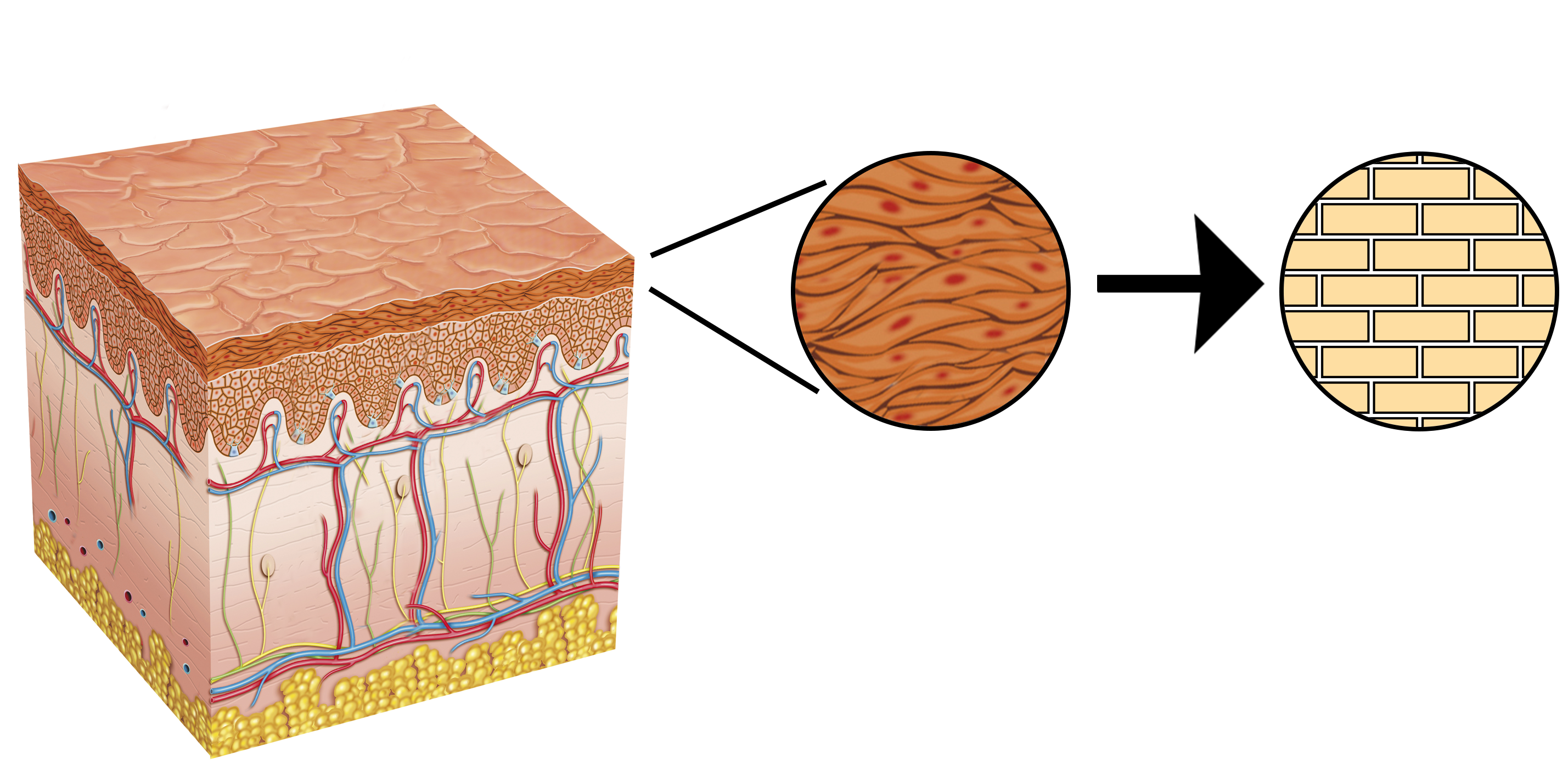
Figure 1: An anatomic representation of the skin, composed by three main layers: epidermis (approximately $100\mu m$ thick), dermis (between $1$ and $3mm$ thick, highly vascularized) and a subcutaneous tissue. The epidermis is divided into sub-layers where the stratum corneum (approximately $15\mu m$ thick) is the outermost layer and is the major barrier to the drug migration, being composed of densely packed cells, with a typical brick and mortar structure. Each skin layer, due to its histological composition, has a different influence in the drug transport mechanism.

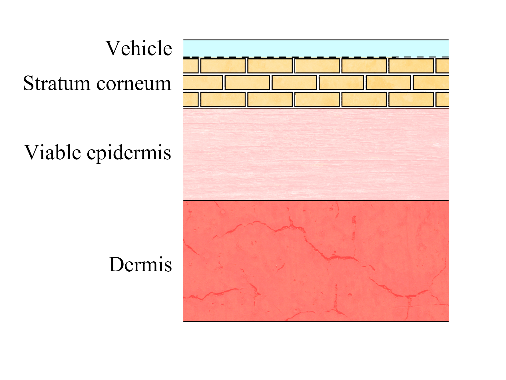
Figure 2: A schematic section representing the present multi-layered model. A vehicle is applied over the skin surface with an imperfect contact at the vehicle-skin interface (figure not to scale).

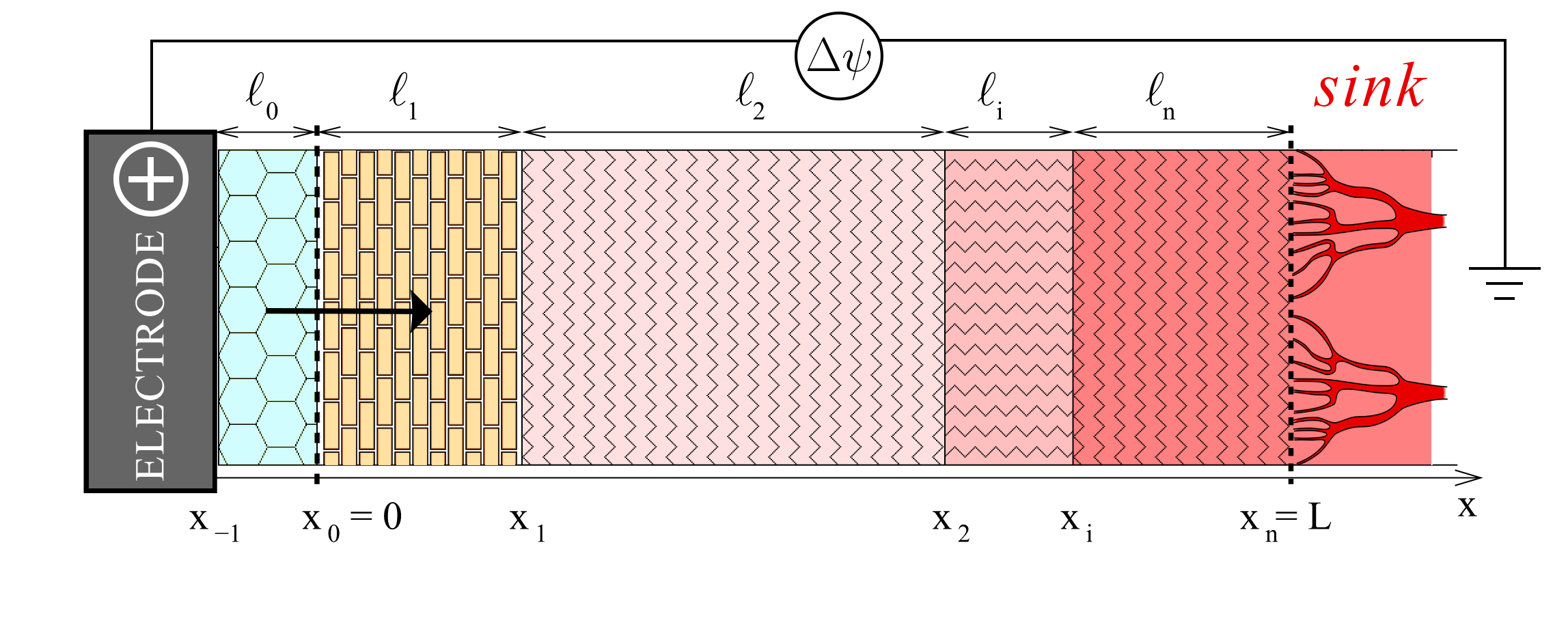
Figure 3: A diagram sketching a $n$-layered tissue ($\ell_{1},\ell_{2},...,\ell_{n}$) faced with the vehicle $\ell_{0}$. The 1D model is defined along the line normal to the skin surface and extends with a sequence of $n$ contiguous layers from the vehicle interface $x_{0}=0$ up to the skin bound $x_{n}=L$, where capillaries sweep the drug away to the systemic circulation (sink). In iontophoresis, a difference of potential is applied to facilitate drug penetration from the vehicle across the tissue’s layers (figure not to scale).

It is well recognized that the skin has a typical composite structure, constituted by a sequence of contiguous layers of different physical properties and thickness, with drug capillary clearance (washout) taking place at the end of it (see [4] for an anatomic and physiological description) (figs 1 - 2). The vehicle (of thickness $\ell_{0}$) and the skin layers (of thicknesses $\ell_{1},\ell_{1},...,\ell_{n}$) are treated as macroscopically homogeneous porous media. Without loss of generality, let us assume that $x_{0}=0$ is the vehicle-skin interface. In a general 1D framework, let us consider a set of intervals $[x_{i-1},x_{i}],\,i=0,1,\dots,n$, having thickness $\ell_{i}=x_{i}-x_{i-1}$, modelling the vehicle (layer 0) and the skin (layers $1,2,\dots,n$), with $L=\sum\limits_{i}\ell_{i}$ the overall skin thickness ($x_{n}=L$) (fig. 3).

At the initial time ($t=0$), the drug is contained only in the vehicle, distributed with maximum concentration $C$ and, subsequently, released into the skin. Here, and throughout this paper, a mass volume-averaged concentration $c_{i}(x,t)$ ($mg/cm^{3}$) is considered in each layer $\ell_{i}$. Since the vehicle is made impermeable with a backing protection, no mass flux pass through the boundary surface at $x=x_{-1}=-\ell_{0}$. Strictly speaking, in a diffusion dominated problem the concentration vanishes asymptotically at infinite distance. However, for computational purposes, the concentration is damped out (within a given tolerance) over a finite distance at a given time. Such a length, (sometimes termed as penetration distance), critically depends on the diffusive properties of the layered medium [24]. At the right end $x=L$ all drug is assumed washed out from capillaries and a sink condition ($c_{n}=0$) is imposed.

3 Transdermal iontophoresis

To promote TDD, an electric field is locally applied in the area where the therapeutic agent has to be released (iontophoresis): one electrode is placed in contact with the vehicle and the other is in contact with the target tissue. To simplify we assume that the drug is positively charged, the anode is at $x=x_{-1}$ and the cathode is at $x=x_{n}$ (fig. 3). Let $\Psi_{0}$ and $\Psi_{1}$, $\Psi_{0}>\Psi_{1}$, be the correspondent applied potential at the endpoints. By mass conservation, the concentration satisfies the following equation:

$${\partial c_{i}\over\partial t}+\nabla\cdot J_{i}=0$$ (3.1)

and in each layer $i$ the mass flux is defined by the Nernst-Planck flux equation [13]:

$$J_{i}=-D_{i}\nabla c_{i}-u_{i}c_{i}\nabla\phi_{i},\,i=0,1,\dots,n$$ (3.2)

where $\phi_{i}$ is the electric potential in layer $i$ and the convective (electroosmotic) term is omitted. Eqn. (3.2) is the generalized Fick’s first law with an additional driving force which is proportional to the electric field. The electric mobility is related to the diffusivity coefficient through the Einstein relation:

$$u_{i}={D_{i}z_{i}F\over RT},\,i=0,1,\dots,n$$ (3.3)

($cm^{2}\,V^{-1}\,s^{-1}$), where $z_{i}$ ion valence, $F$ the Faraday constant, $R$ the gas constant, $T$ the absolute temperature. The boundary conditions are

$$J_{0}=0\qquad\mbox{at}\quad x=-\ell_{0}=-x_{-1}\qquad\mbox{(impermeable backing)}$$ (3.4)

$$c_{n}=0\qquad\mbox{at}\quad x=x_{n}\qquad\mbox{(sink condition due to the capillary washout)}$$ (3.5)

The last condition arises because, in deep skin, drug is uptaken by capillary network and is lost in the systemic circulation: we refer to this as systemically absorbed (shortly “absorbed” ) drug. At $x=0$ we impose the matching of the total fluxes and that they are proportional to the jump of concentration (Kedem-Katchalski eqn):

$$J_{0}=J_{1}=P(c_{0}-c_{1})\qquad\mbox{at}\quad x=0$$ (3.6)

with $P$(cm/s) a mass transfer coefficient (includes a drug partitioning and a mass flux resistance). At the other interfaces we assume a perfect contact and continuity of concentrations and fluxes:

$$J_{i}=J_{i+1}\qquad\qquad c_{i}=c_{i+1}\qquad\mbox{at}\quad x=x_{i},\qquad\quad i=1,2,\dots,n-1$$ (3.7)

The initial conditions are set as:

$$c_{0}(x,0)=C,\qquad c_{i}(x,0)=0\qquad i=1,2,\dots,n$$ (3.8)

3.1 The electric potential field

To solve equations (3.1)–(3.3), in some cases the potential $\phi$ is assigned, but in this multi-layer system we find it as solution of the Poisson equation:

$$\nabla\cdot(\sigma_{i}\nabla\phi_{i})=\sum_{k}z_{k}c_{k}\simeq 0\qquad i=0,1,\dots,n$$ (3.9)

$$\phi_{0}=\Psi_{0}\qquad\mbox{at}\quad x=-x_{-1}$$ (3.10)

$$\phi_{n}=\Psi_{1}\qquad\mbox{at}\quad x=x_{n}$$ (3.11)

with $\sigma_{i}(\displaystyle{cm^{-1}\,\Omega^{-1}})$ the electrical conductivities in the layer $i$ [8]. At the interfaces we assume an electrically perfect contact and we have continuity of potential and fluxes:

$$-\sigma_{i}\nabla\phi_{i}=-\sigma_{i+1}\nabla\phi_{i+1}\qquad\qquad\phi_{i}=\phi_{i+1}\qquad\mbox{at}\quad x=x_{i}\qquad i=0,1,\dots,n-1$$ (3.12)

It is straightforward to verify that the exact solution of the problem (3.9)–(3.12) is

$$\phi_{i}(x)=a_{i}x+b_{i}\qquad i=0,1,\dots,n$$ (3.13)

with the expressions of $a_{i}(V/cm)$ and $b_{i}(V)$ are computed in the specific cases (see sect. 7).

4 Energy estimates

In this section we establish some energy estimates in the two cases of finite $P>0$ (subsection 4.1) and in the limit case $P\rightarrow\infty$ (subsection 4.2) at interface condition (3.6), that leads to upper bound of total drug masses. These results will be used to obtain stability and uniqueness results under a condition on the applied potential and on the diffusivities. We point out that our analysis concerns the global energy as well as the total mass of drug in the whole system, and cannot be carried out in the single layers.

4.1 The general case: imperfect contact

Let $(\cdot,\cdot)_{i}$ be the usual inner product in $L^{2}(x_{i-1},x_{i})$ and $\|\cdot\|_{i}$ the corresponding norm, $i=0,\dots,n.$ From (3.1) we deduce

$$\sum_{i=0}^{n}\left(\frac{\partial c_{i}}{\partial t},c_{i}\right)_{i}+\sum_{i=0}^{n}(\nabla\cdot J_{i},c_{i})_{i}=0.$$ (4.1)

Combining (4.1) with the boundary conditions (3.4)–(3.5) and the interface conditions (3.6), (3.7) we get

$$\frac{1}{2}\xi^{\prime}(t)+\sum_{i=0}^{n}D_{i}\|\nabla c_{i}\|_{i}^{2}+\sum_{i=0}^{n}(v_{i}c_{i},\nabla c_{i})_{i}=-P\big{(}c_{0}(0,t)-c_{1}(0,t)\big{)}^{2}$$ (4.2)

where $v_{i}=u_{i}\nabla\phi_{i},$ is the convective velocity induced by the potential field, and $\xi(t)=\sum\limits_{i=0}^{n}\|c_{i}(t)\|_{i}^{2}$ is the total energy. By the Young inequality we have:

$$(v_{i}c_{i},\nabla c_{i})_{i}\geq-\frac{1}{4\epsilon^{2}}v_{i}^{2}\|c_{i}\|_{i}^{2}-\epsilon_{i}^{2}\|\nabla c_{i}\|_{i}^{2},$$

for any $\epsilon_{i}\neq 0.$ Then from (4.2) we get

$$\frac{1}{2}\xi^{\prime}(t)+\sum_{i=0}^{n}\Big{(}D_{i}-\epsilon_{i}^{2}\Big{)}\|\nabla c_{i}\|_{i}^{2}-\sum_{i=0}^{n}\frac{v_{i}^{2}}{\epsilon_{i}^{2}}\|c_{i}\|_{i}^{2}\leq-P\big{(}c_{0}(0,t)-c_{1}(0,t)\big{)}^{2}$$ (4.3)

Taking $\epsilon_{i}^{2}=D_{i}$ in (4.3) we obtain:

$$\xi^{\prime}(t)-2\sum_{i=0}^{n}\frac{v_{i}^{2}}{D_{i}}\|c_{i}\|_{i}^{2}\leq-2P\big{(}c_{0}(0,t)-c_{1}(0,t)\big{)}^{2}.$$ (4.4)

Finally, (4.4) leads to

$$\xi(t)\leq e^{{\alpha}t}\Big{(}\xi(0)-2P\int_{0}^{t}e^{-{\alpha}s}\big{(}c_{0}(0,s)-c_{1}(0,s)\big{)}^{2}ds\Big{)}.$$ (4.5)

with $\alpha=2\max\limits_{i=0,\dots,n}\displaystyle\frac{v_{i}^{2}}{D_{i}}.$ The upper bound (4.5) shows that the initial boundary value problem (3.1)– (3.8) is stable for finite t. Through the previous inequality, we prove the uniqueness of the solution as follows: if we assume that in each sub-interval we have at least two solutions $c_{i}$ and $\tilde{c}_{i}$ that satisfy the same initial condition, then for $w_{i}=c_{i}-\tilde{c}_{i}$ we have

$$\xi(t)\leq e^{{\alpha}t}\Big{(}-2P\int_{0}^{t}e^{-{\alpha}s}\big{(}w_{0}(0,s)-w_{1}(0,s)\big{)}^{2}ds\Big{)}.$$ (4.6)

This means that $\xi(t)\leq 0$ and consequently $c_{i}=\tilde{c}_{i},i=0,\dots,n.$ The existence of the solution is guaranteed by showing that an analytic solution can be built as a Fourier series, analogously to similar diffusion-convective problems in layered systems [18].

The upper bound (4.5) can be used to describe the behavior of the coupled system for the released mass. Let

$$M_{i}(t)=\int_{x_{i-1}}^{x_{i}}c_{i}(s)ds\qquad M(t)=\sum_{i=0}^{n}M_{i}(t)$$ (4.7)

be the mass in the layer $i$ and the total mass, respectively. Being $\displaystyle M(t)^{2}\leq\xi(t)L$ , we get, from equation (4.6), the following upper bound for the drug mass in the coupled system

$$M(t)\leq\sqrt{L}e^{{\alpha\over 2}t}\Big{(}\xi(0)-2P\int_{0}^{t}e^{-{\alpha}s}\big{(}c_{0}(0,s)-c_{1}(0,s)\big{)}^{2}ds\Big{)}^{1/2}.$$ (4.8)

This estimate shows that the larger is $P$, the smaller is the total mass (i.e. the larger is the absorbed mass). The above bound depends on the history of concentration jump at contact interface weighted by controllable quantities such as the applied potential and the media diffusivities.

4.2 The limit case $P\rightarrow\infty$: perfect contact

We now consider the limit case of $P$, that is when the contact between the vehicle and the target tissue is perfect, and allows the continuity of the concentration in the interface between both media. Differently from the previous subsection, the regularity of the concentration allows the use the Poincaré inequality. Let $D$, $v$ and $c$ be defined by:

$$D(x)=D_{i},\qquad\quad v(x)=v_{i},\qquad\quad c(x,t)=c_{i}(x,t),\qquad\quad x\in(x_{i-1},x_{i}),\,i=0,\dots,n.$$

with (3.6) replaced by:

$$J_{0}=J_{1},\,\quad c_{0}=c_{1}\qquad\mbox{at}\quad x=0,$$ (4.9)

Let $(\cdot,\cdot)$ be the usual inner product in $L^{2}(x_{-1},x_{n})$ and let $\|\cdot\|$ the corresponding norm. We start by observing that we have

$$\frac{1}{2}\xi^{\prime}(t)=-(D\nabla c(t),\nabla c(t))-(vc(t),\nabla c(t)).$$ (4.10)

Being

$$-(vc(t),\nabla c(t))\leq\max_{i=0,\dots,n}|v_{i}|\|c(t)\|\|\nabla c(t)\|,$$

and taking into account the following Poincairé inequality $\xi(t)\leq\displaystyle\frac{L^{2}}{2}\|\nabla c(t)\|^{2},$ we obtain

$$-(vc(t),\nabla c(t))\leq\max_{i=0,\dots,n}|v_{i}|\frac{L}{\sqrt{2}}\|\nabla c(t)\|^{2}.$$

Inserting the last upper bound in (4.10) we deduce

$$\xi^{\prime}(t)\leq\Big{(}-2\min_{i=0,\dots,n}D_{i}+\max_{i=0,\dots,n}|v_{i}|\sqrt{2}L\Big{)}\|\nabla c(t)\|^{2}.$$ (4.11)

If

$$\max_{i=0,\dots,n}\frac{|v_{i}|}{D_{i}}L\leq\sqrt{2}.$$ (4.12)

by applying the Poincaré inequality in (4.11), we get

$$\xi(t)\leq e^{\beta t}\|c(0)\|^{2},$$ (4.13)

where

$$\beta=\frac{1}{L^{2}}\Big{(}-2\min_{i=0,\dots,n}D_{i}+\max_{i=0,\dots,n}|v_{i}|\sqrt{2}L\Big{)}.$$

Under the condition (4.12) we get the mass upper bound:

$$M(t)\leq\sqrt{L}e^{\beta t}\|c(0)\|.$$ (4.14)

From equation (4.14), the decreasing of the upper bound for the drug mass $M(t)$ is observed provided that (4.12) holds.

5 Nondimensional equations

Before solving the differential problem, all the variables, the parameters and the equations are now normalized to get easily computable nondimensional quantities as follows:

$$\bar{x}={x\over L}\qquad\qquad\bar{t}={D_{max}\over L^{2}}t\qquad\qquad\bar{c}_{i}={c_{i}\over C}\qquad\qquad\delta={l_{0}\over L}$$

$$\gamma_{i}={D_{i}\over D_{max}}\qquad\qquad\bar{\phi}_{i}={Fz_{i}\over RT}\phi_{i}\qquad\qquad\Pi={PL\over D_{max}}$$ (5.1)

where the subscript $\max$ denotes the maximum value across the $n+1$ layers. By omitting the bar for simplicity, the 1D nondimensional Nernst-Planck equations (3.1)–(3.2) become:

$${\partial c_{i}\over\partial t}=\gamma_{i}{\partial^{2}c_{i}\over\partial x^{2}}+\gamma_{i}\left({\partial c_{i}\over\partial x}{\partial\phi_{i}\over\partial x}+c_{i}{\partial^{2}\phi_{i}\over\partial x^{2}}\right)=\gamma_{i}{\partial^{2}c_{i}\over\partial x^{2}}+\gamma_{i}a_{i}{\partial c_{i}\over\partial x}\qquad i=0,1,\dots,n$$ (5.2)

(cfr. with (3.13)). The above eqns are supplemented by the following boundary/interface conditions:

$$J_{0}=-\gamma_{0}\left({\partial c_{0}\over\partial x}+a_{0}c_{0}\right)=0\qquad \mbox{at}\quad x=-\delta$$ (5.3)

$$J_{0}=-\gamma_{0}\left({\partial c_{0}\over\partial x}+a_{0}c_{0}\right)=-\gamma_{1}\left({\partial c_{1}\over\partial x}+ac_{1}\right)=J_{1}$$

$$J_{0}=-\gamma_{0}\left({\partial c_{0}\over\partial x}+a_{0}c_{0}\right)=\Pi(c_{0}-c_{1})\qquad \mbox{at}\quad x=0$$ (5.4)

$$J_{i}=-\gamma_{i}\left({\partial c_{i}\over\partial x}+ac_{i}\right)=-\gamma_{i+1}\left({\partial c_{i+1}\over\partial x}+ac_{i+1}\right)=J_{i+1}$$

$$c_{i}=c_{i+1}\qquad i=1,\dots,n-1\qquad \mbox{at}\quad x=x_{i}$$ (5.5)

$$c_{n}=0\qquad \mbox{at}\quad x=1$$ (5.6)

and initial conditions:

$$c_{0}(x,0)=1\qquad\qquad\qquad c_{i}(x,0)=0\quad i=1,2,\dots,n$$ (5.7)

6 Numerical solution

Although a semi-analytic treatment is possible in multi-layered diffusion problems [24], we proceed to solve the nondimensional system of equations (5.2)–(5.6) numerically. Let us subdivide the interval $(-\delta,0)$ into $N_{0}+1$ equispaced grid nodes $x_{0}^{j}=(j-N_{0})\,h_{0},\quad j=0,1,\dots,N_{0}$, and the $i-$th interval $[x_{i},x_{i+1}]$ with $N_{i}+1$ equispaced points $x_{i}^{j}=j\,h_{i},\quad j=0,1,\dots,N_{i}$. Here, $h_{0},h_{1},h_{2}\dots,h_{n}$ represent the spacing in the vehicle (layer 0) and skin (layers $i=1,2\dots,n$), respectively. In each layer, we approximate the diffusive terms by considering a standard finite-difference of the second derivative and centered first derivative at internal nodes $x_{j}$:

$$\left.{\partial c_{i}\over\partial x}\right|_{x_{j}}\simeq{c_{i}^{j+1}-c_{i}^{j-1}\over 2h_{i}}$$

$$\left.{\partial^{2}c_{i}\over\partial x^{2}}\right|_{x_{j}}\simeq{c_{i}^{j-1}-2c_{i}^{j}+c_{i}^{j+1}\over h_{i}^{2}}\qquad\qquad j=1,\dots,N_{i}-1\qquad i=0,1,\dots,n$$

At the boundary points $x=-\delta$ and $x=1$ and at interfaces $x_{i}$, the equations (5.2) hold, but the approximations (LABEL:ev1) include the boundary conditions (5.3)–(5.6) and the interface conditions (5.5).

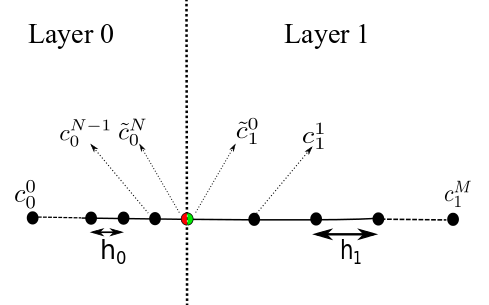
Figure 4: Schematic illustration of grid nodes in the first two layers and the interface points (in red and green). They are computed a posteriori as a linear combination of the neighbouring grid points (eqns. (6.4)–(6.5)). At the other interfaces a single concentration values occur.

Treatment of the interface $x=0$
At the interface $x=0$, we potentially have a discontinuity in concentration and two possibly different values, say $\tilde{c}_{0}^{N}$ and $\tilde{c}_{1}^{0}$ (the tilde accent indicates these special points) , each for each interface side, need to be determined (fig. 4).

No derivative can be computed across the interface $x=0$, due to a possible discontinuity and approximations (LABEL:ev1) no longer apply. An alternative procedure is needed in eqn (LABEL:ev1) to get $\tilde{c}_{0}^{N}$ for $j=N_{0}-1$ and $\tilde{c}_{1}^{0}$ for $j=1$. Their values are related through the interface conditions (5.4):

$$-\gamma_{0}\left({\partial\tilde{c}_{0}^{N}\over\partial x}+a_{0}\tilde{c}_{0}^{N}\right)=-\gamma_{1}\left({\partial\tilde{c}_{1}^{0}\over\partial x}+a\tilde{c}_{1}^{0}\right)$$

$$-\gamma_{0}\left({\partial\tilde{c}_{0}^{N}\over\partial x}+a_{0}\tilde{c}_{0}^{N}\right)=\Pi(\tilde{c}_{0}^{N}-\tilde{c}_{1}^{0})$$ (6.2)

Following the approach described by Hickson et al. [25] , we take a Taylor series expansion for $c_{0}^{N-2},c_{0}^{N-1},c_{1}^{1},c_{1}^{2}$, and arrive at:

$$c_{0}^{N-1}\approx\tilde{c}_{0}^{N}-h_{0}{\partial\tilde{c}_{0}^{N}\over\partial x}+{h_{0}^{2}\over 2}{\partial^{2}\tilde{c}_{0}^{N}\over\partial x^{2}}$$

$$c_{0}^{N-2}\approx\tilde{c}_{0}^{N}-2h_{0}{\partial\tilde{c}_{0}^{N}\over\partial x}+2{h_{0}^{2}}{\partial^{2}\tilde{c}_{0}^{N}\over\partial x^{2}}$$

$$c_{1}^{1}\approx\tilde{c}_{1}^{0}+h_{1}{\partial\tilde{c}_{1}^{0}\over\partial x}+{h_{1}^{2}\over 2}{\partial^{2}\tilde{c}_{1}^{0}\over\partial x^{2}}$$

$$c_{1}^{2}\approx\tilde{c}_{1}^{0}+2h_{1}{\partial\tilde{c}_{1}^{0}\over\partial x}+2{h_{1}^{2}}{\partial^{2}\tilde{c}_{1}^{0}\over\partial x^{2}}$$ (6.3)

The two equations (6.2) and the four equations (6.3) form an algebraic system of six equations that allow to express $\tilde{c}_{0}^{N},\tilde{c}_{1}^{0}$ and their first and second derivatives as a linear combination of the neighboring values. Using symbolic calculus we obtain:

$$\tilde{c}_{0}^{N}={[\gamma_{0}\gamma_{1}(3-2ah_{1})+2\Pi\gamma_{0}h_{1}](c_{0}^{N-2}-4c_{0}^{N-1})+2\gamma_{1}h_{0}\Pi(c_{1}^{2}-4c_{1}^{1})\over Q}$$ (6.4)

$$\tilde{c}_{1}^{0}={[\gamma_{0}\gamma_{1}(3+2a_{0}h_{0})+2\Pi\gamma_{1}h_{0}](c_{1}^{2}-4c_{1}^{1})+2\gamma_{0}h_{1}\Pi(c_{0}^{N-2}-4c_{0}^{N-1})\over Q}$$ (6.5)

where $Q=2\gamma_{1}h_{0}\Pi(2ah_{1}-3)+\gamma_{0}(2a_{0}h_{0}+3)(2a\gamma_{1}h_{1}-3\gamma_{1}-2h_{1}\Pi)$.

After spatial discretization, the system of PDEs reduces to a system of nonlinear ordinary differential equations (ODEs) of the form:

$${dY\over dt}=A(Y)$$ (6.6)

where $Y=(c_{0}^{0},\dots.,c_{0}^{N-1},c_{1}^{1},\dots,c_{1}^{N_{1}},\dots.,c_{n}^{0},\dots.c_{n}^{N_{n}})^{T}$ and $A(Y)$ contains the coupled $N_{0}+N_{1}+\dots+N_{n}$ discretized equations (5.2). The system (6.6) is solved by the routine ode15s of Matlab based on a Runge-Kutta type method with backward differentiation formulas, and an adaptive time step. The interface drug concentrations $\tilde{c}_{0}^{N},\tilde{c}_{1}^{0}$ are computed a posteriori through equations (6.4)–(6.5).

7 Results and discussion

A common difficulty in simulating physiological processes, in particular TDD, is the identification of reliable estimates of the model parameters. Experiments of TDD are impossible or prohibitively expensive in vivo and the only available source are lacking and incomplete data from literature. The drug delivery problem depends on a large number of constants, each of them varies in a finite range, with a variety of combinations and limiting cases. Furthermore, these parameters can be influenced by body delivering site, patient age and individual variability. They cannot be chosen independently from each other and there is a compatibility condition among them.

Here, the skin is assumed to be composed of three main layers, say the stratum corneum, the viable epidermis, and the dermis with respective model parameters given in table 1. In the absence of direct measurements, indirect data are inferred from previous studies in literature [4, 7, 26]. Diffusivities critically depend on the kind and size of the transported molecules and are affected of a high degree of uncertainty. The vehicle-skin permeability parameter is estimated as $P=10^{-5}cm/s$.

Table 1: The parameters used in the simulations for the vehicle and the three skin layers.

—	vehicle (0)	stratum corneum (1)	viable epidermis (2)	dermis (3)
$l_{i}=x_{i}-x_{i-1}(cm)$	$0.01$	$1.75\cdot 10^{-3}$	$3.5\cdot 10^{-3}$	$0.11$
$D_{i}(cm^{2}/s)$	$10^{-4}$	$10^{-10}$	$10^{-7}$	$10^{-7}$
$\sigma_{i}(S/cm)$	$1.5\cdot 10^{-2}$	$10^{-7}$	$10^{-4}$	$10^{-4}$

The coefficients of potential $\phi_{i}$ in eqn (3.13) have the following expressions:

$$a_{0}=-{\Delta\Psi\sigma_{1}\sigma_{2}\sigma_{3}\over G}$$

$$b_{0}={l_{0}\Psi_{1}\sigma_{1}\sigma_{2}\sigma_{3}+l_{1}\Psi_{0}\sigma_{0}\sigma_{3}(\sigma_{2}-\sigma_{1})+l_{2}\Psi_{0}\sigma_{0}\sigma_{1}(\sigma_{3}-\sigma_{2})+l_{3}\Psi_{0}\sigma_{0}\sigma_{1}\sigma_{2}\over G}$$

$$a_{1}=-{\Delta\Psi\sigma_{0}\sigma_{2}\sigma_{3}\over G}$$

$$b_{1}={l_{0}\Psi_{1}\sigma_{1}\sigma_{2}\sigma_{3}+l_{1}\Psi_{0}\sigma_{0}\sigma_{3}(\sigma_{2}-\sigma_{1})+l_{2}\Psi_{0}\sigma_{0}\sigma_{1}(\sigma_{3}-\sigma_{2})+l_{3}\Psi_{0}\sigma_{0}\sigma_{1}\sigma_{2}\over G}=b_{0}$$

$$a_{2}=-{\Delta\Psi\sigma_{0}\sigma_{1}\sigma_{3}\over G}$$

$$b_{2}={l_{0}\Psi_{1}\sigma_{1}\sigma_{2}\sigma_{3}+l_{1}\Psi_{1}\sigma_{0}\sigma_{3}(\sigma_{2}-\sigma_{1})+l_{2}\Psi_{0}\sigma_{0}\sigma_{1}(\sigma_{3}-\sigma_{2})+l_{3}\Psi_{0}\sigma_{0}\sigma_{1}\sigma_{2}\over G}$$

$$a_{3}=-{\Delta\Psi\sigma_{0}\sigma_{1}\sigma_{2}\over G}$$

$$b_{3}={l_{0}\Psi_{1}\sigma_{1}\sigma_{2}\sigma_{3}+l_{1}\Psi_{1}\sigma_{0}\sigma_{3}(\sigma_{2}-\sigma_{1})+l_{2}\Psi_{1}\sigma_{0}\sigma_{1}(\sigma_{3}-\sigma_{2})+l_{3}\Psi_{0}\sigma_{0}\sigma_{1}\sigma_{2}\over G}$$ (7.1)

where $G=l_{0}\sigma_{1}\sigma_{2}\sigma_{3}+l_{1}\sigma_{0}\sigma_{3}(\sigma_{2}-\sigma_{1})+l_{2}\sigma_{0}\sigma_{1}(\sigma_{3}-\sigma_{2})+l_{3}\sigma_{0}\sigma_{1}\sigma_{2}$ and $\Delta\Psi=\Psi_{0}-\Psi_{1}$. Note that only the electric potential gradients, $a_{i}$, appear in the Nernst-Planck equation and the ratio of the slopes satisfies: $\displaystyle{a_{i}\over a_{i+1}}=\displaystyle{\sigma_{i+1}\over\sigma_{i}}$.

Instead than reproducing the clinical protocols where iontophoresis consists in repeated sessions of 10-20 mins, the numerical simulations aim at bringing to extreme values both the potential (up to $\Delta\Psi=10V$) and the duration of application (30 mins): a current is activated during this period of time and then switched off. In fig. 5 the concentration profiles are shown before (continuous lines) and after (dashed lines) the current application. The iontophoretic effect is to enhance the stratum corneum permeation but, only for higher $\Delta\Psi$, appears to be significant in deeper layers. No relevant effect is present after suspension. It is desirable the drug level is maintained over a certain amount to exerts its therapeutic effect without exceeding a given threshold to not be toxic.

In fig. 6 the different distribution of drug mass in all layers is depicted: mass is decreasing in the vehicle, whereas in the other layers is first increasing, reaches a peak, and asymptotically decreasing, as in other similar drug delivery systems [18, 24]. Due to the sink condition at the right end, part of mass is lost via the systemic circulation. By considering this effect, a drug mass conservation holds and the progressive emptying of the vehicle corresponds to the drug replenishment of the other layers – in a cascade sequence – at a rate depending of the electric field (fig. 6). Again, an augmented transdermal permeation is reported with higher values of the potential: this is more effective during current administration, but prolongs at later times ($12h-72h$). The transport of a species across skin will be determined by the strength and the duration of the electric field, the concentration and the mobility of all ions in the skin. The desired delivery rate is obtained with a proper choice of the physico-chemical-electrical parameters.

These outcomes provide valuable indications to assess whether drug reaches a deeper layer, and to optimize the dose capacity in the vehicle. Therefore, it is possible to identify the conditions that guarantee a more prolonged and uniform release or a localized peaked distribution.

8 Conclusions

Nowadays iontophoretic systems are commonly used in transdermal applications. These systems use an electric field to enhance the release from a drug reservoir and to direct the therapeutic action at the target tissue with a given rate and at desired level. Iontophoresis provides a mechanism to control the transport of hydrophilic and charged agents across the skin, especially for high molecular weight substances such as peptides or proteins which are usually ionized and hardly penetrate the stratum corneum by conventional passive diffusion. Notwithstanding, the effective utilization of electric field-assisted transport for drug delivery across biological membranes requires a deeper understanding of the mechanisms and theories behind the process.

In this paper a multi-layer model is developed to clarify the role of the applied potential, the conductivity of the skin, the drug diffusion and the systemic absorption. The stability of the mathematical problem is discussed within two different scenarios: imperfect and perfect contact between the reservoir and the target tissue. To illustrate the drug dynamics in the composite medium - vehicle and skin layers coupled - during and after the electric administration, an accurate finite-difference method is proposed. The modelling approach allows the simulation in several experimental setting, including extreme conditions which are not possible in clinical environment. Numerical experiments show to what extent the applied current, along the duration of application, accelerates the depletion of the reservoir and increases the drug absorption in the deep skin. The present TDD model constitutes a simple and useful tool in exploring new delivering strategies that guarantee the optimal and localized release for an extended period of time.

	$c_{0}$	$c_{1}$	$c_{2}$	$c_{3}$
$\Delta\Psi=0V$
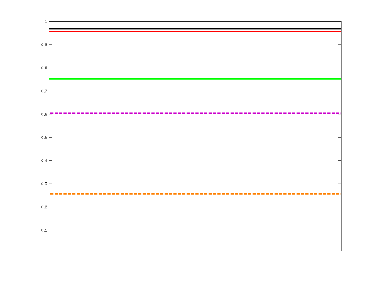
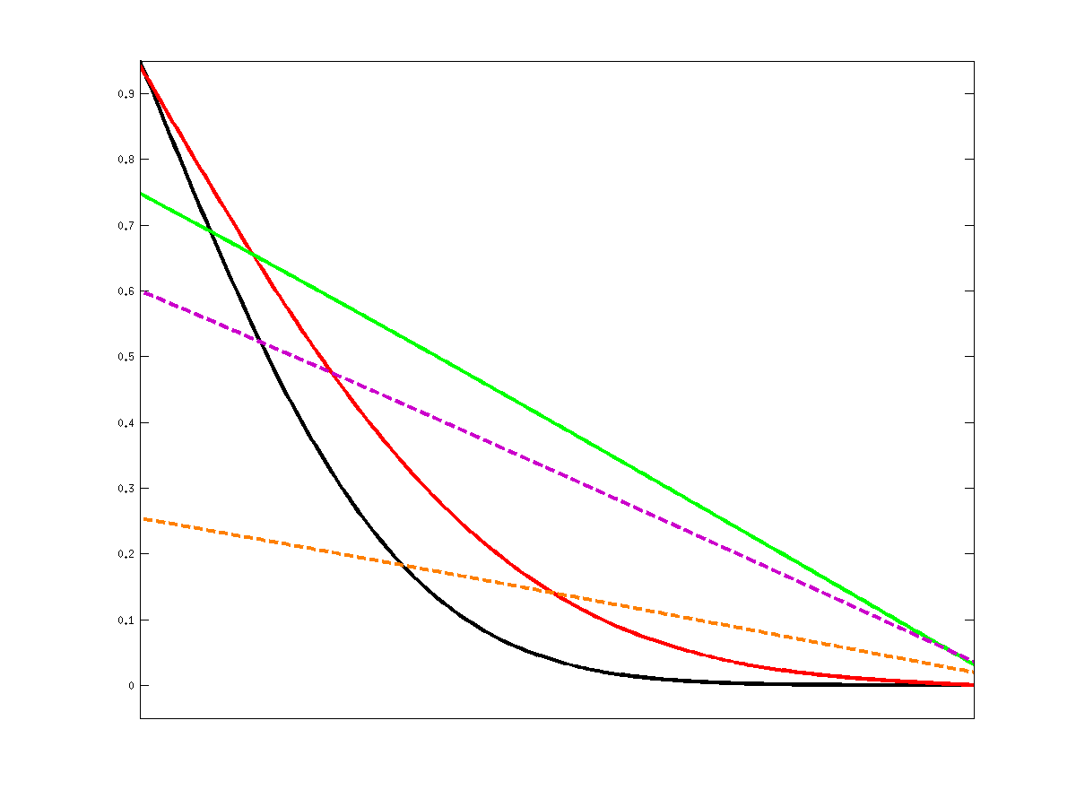
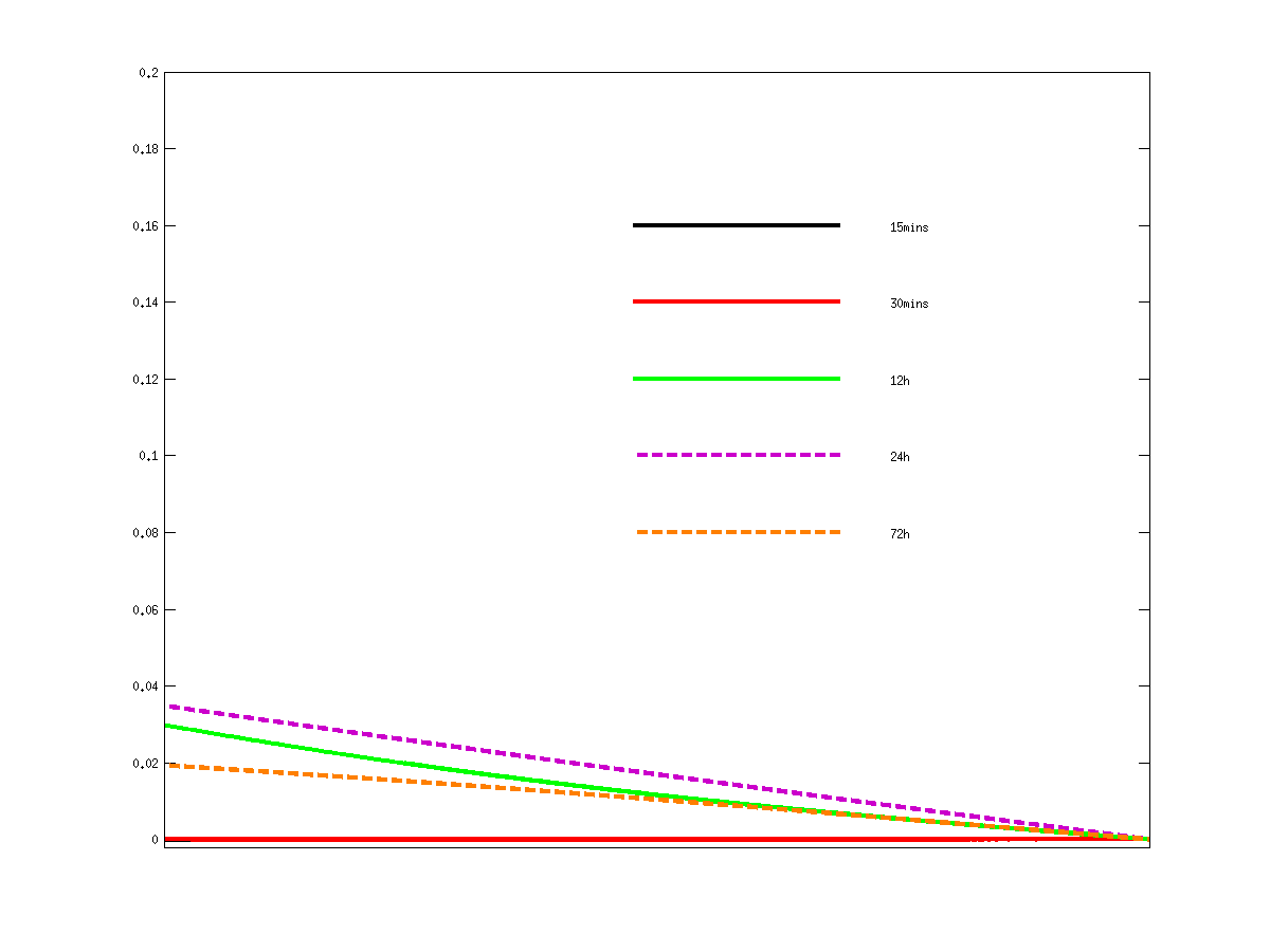
$\Delta\Psi=1V$
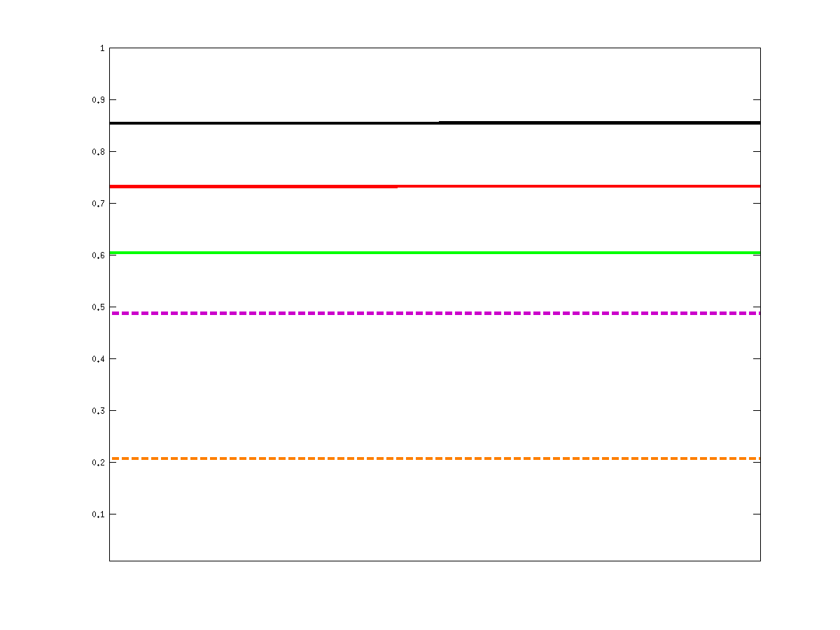
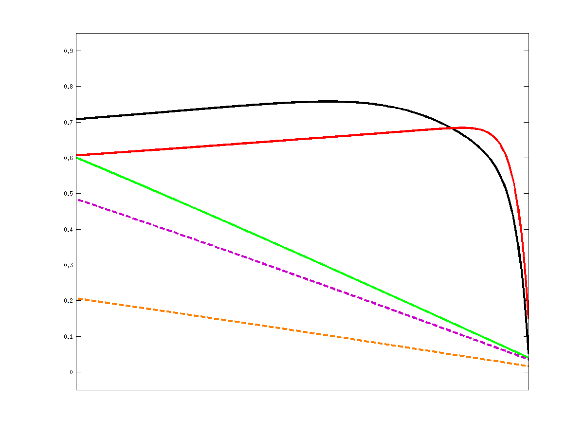
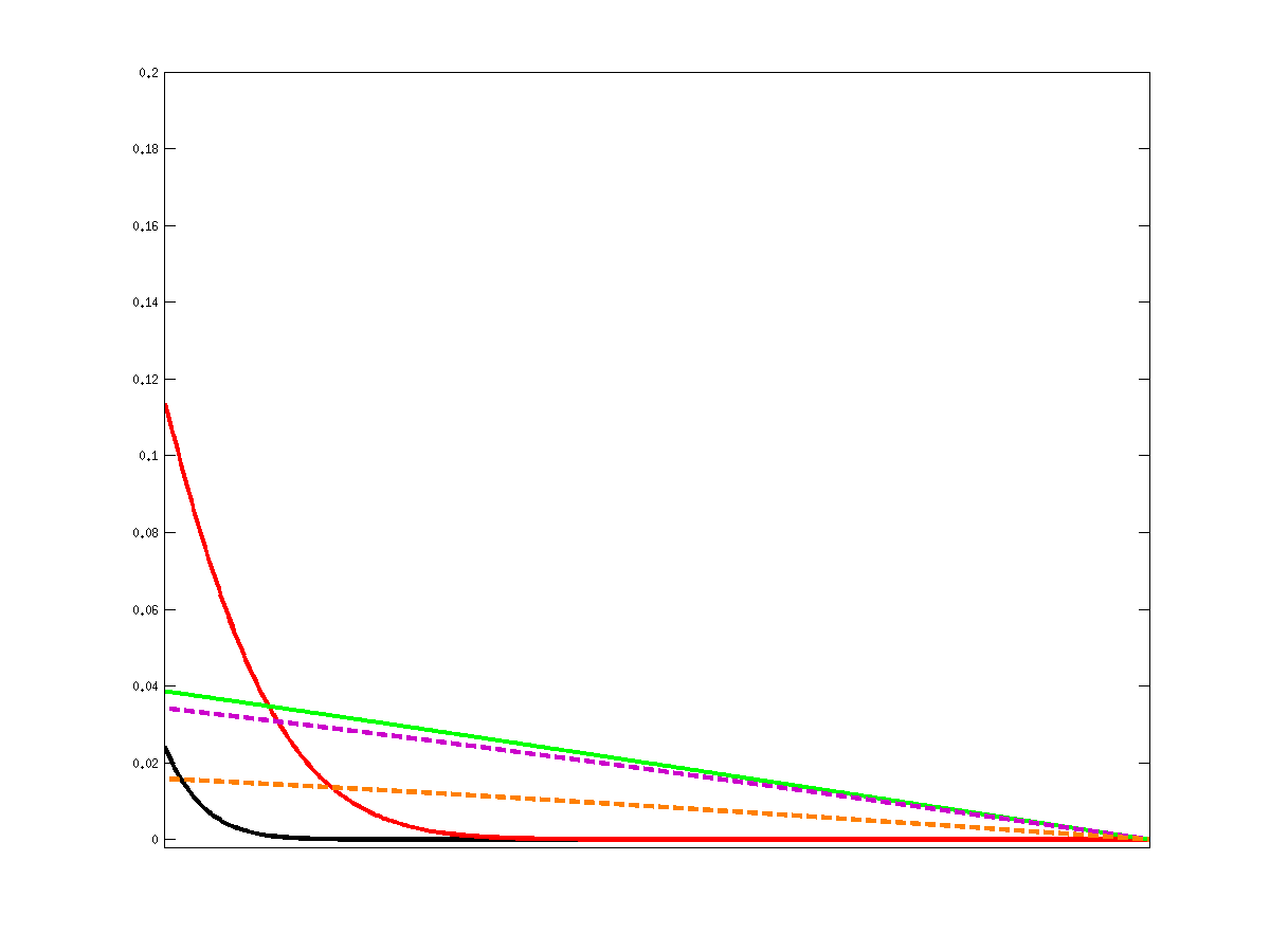
$\Delta\Psi=10V$

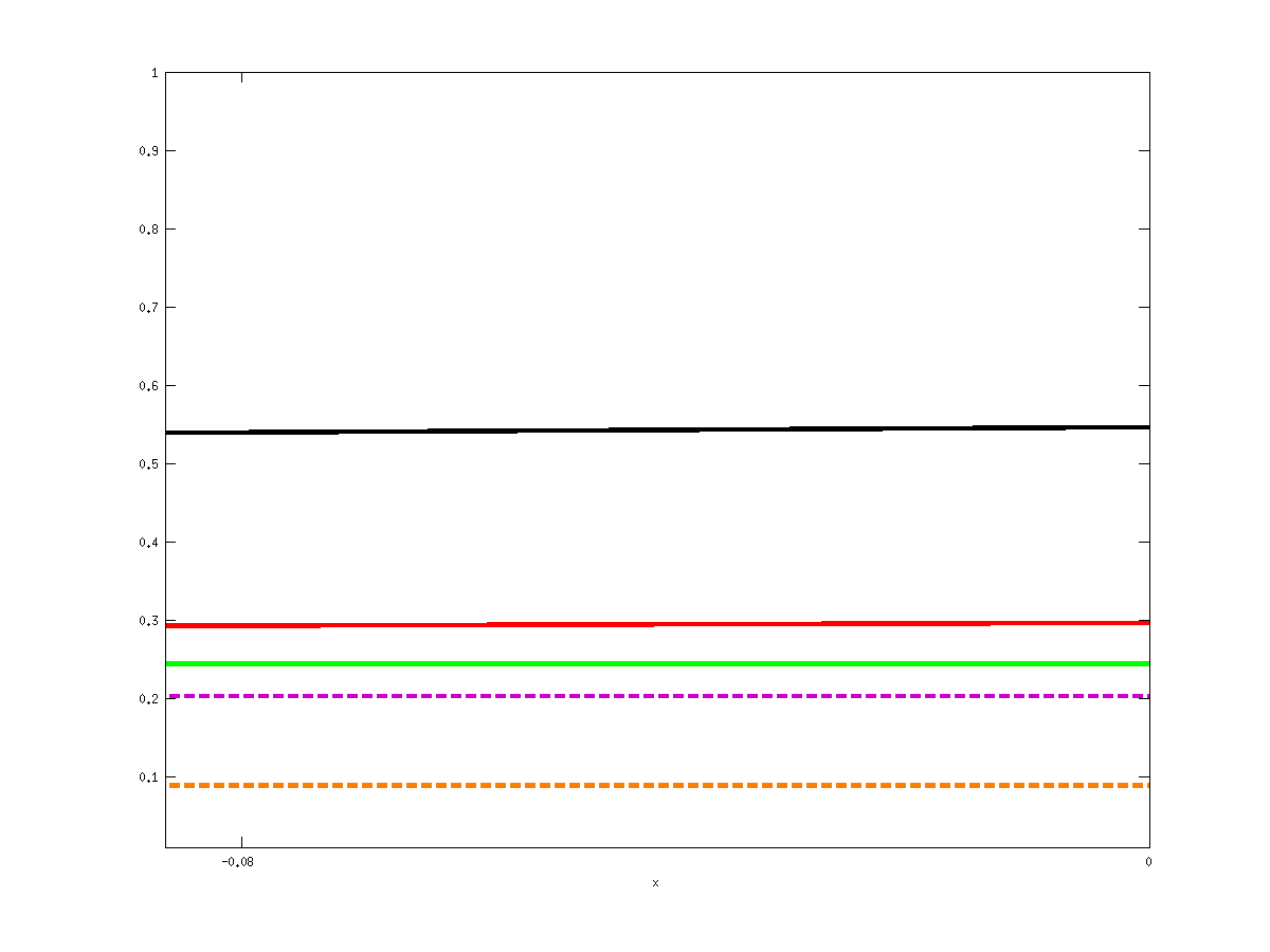
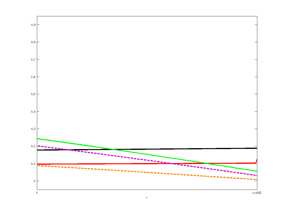
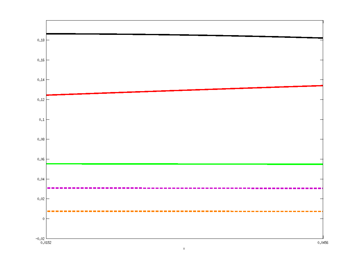
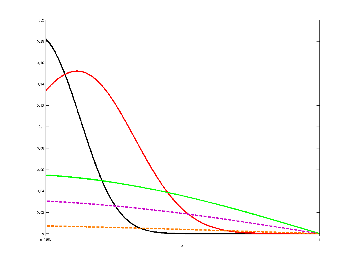
Figure 5: Profiles of concentration in all layers at five times (continuous lines during current administration, dashed lines after suspension), for three differences of potential. The effect of iontophoresis is to enhance penetration in the stratum corneum, and for higher voltage, even in the deeper layers (simulations based on a uniform mesh size $h_{0}=h_{1}=h_{2}=h_{3}=2\cdot 10^{-3}$, current switched off after 30min).

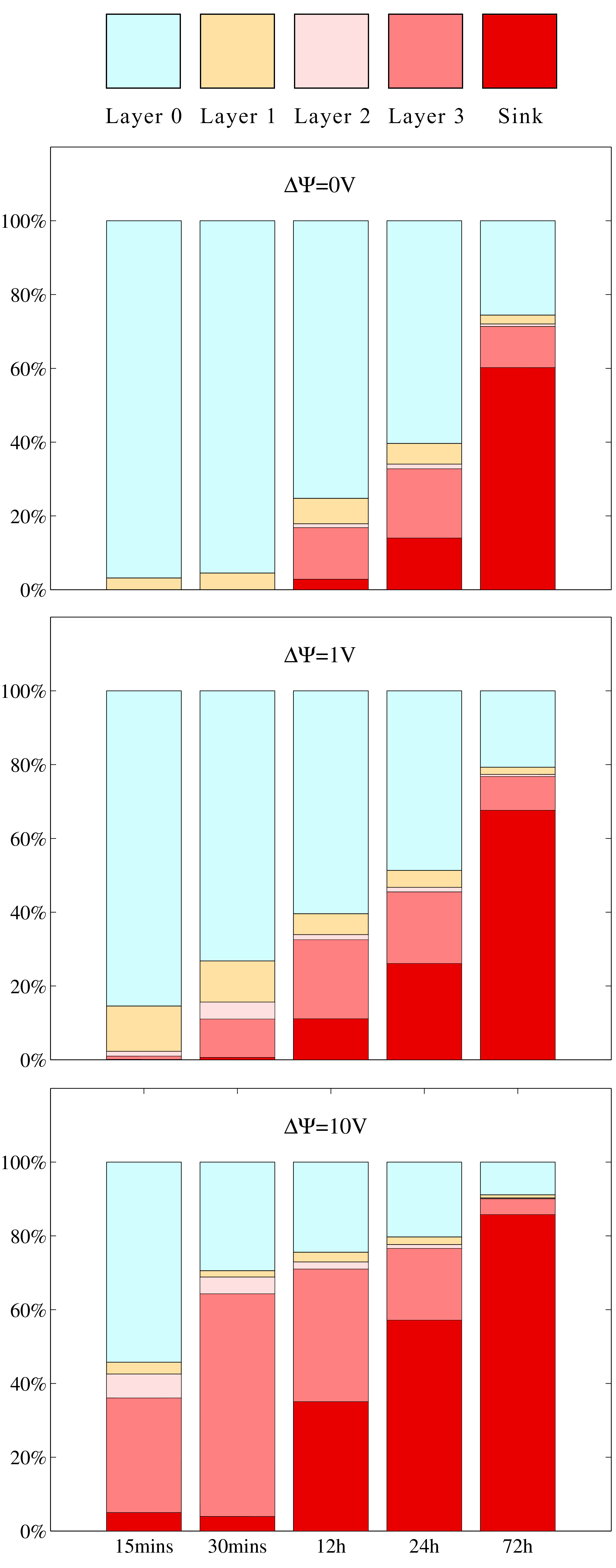
Figure 6: Distribution of mass in all layers (including the vehicle (layer 0) and the sink) at five times, for three differences of potential. The heights of the rectangles indicate the percentage of mass retained in each layer. A higher current accelerates depletion of the vehicle and enhances drug delivery in stratum corneum and in the deeper skin’s layers. At later times most of drug results absorbed at the systemic level (current switched off after 30min).

References

- [1] M. Prausnitz, S. Mitragori, R. Langer, Current status and future potential of transdermal drug delivery, Nature Reviews, Drug Discovery, 3, 115-124, 2004.
- [2] H. Trommer, R. Neubert, Overcoming the stratum corneum: the modulation of skin penetration, Skin Pharmacology and Physiology, 19, 106–121, 2006.
- [3] M. Prausnitz, R. Langer, Transdermal drug delivery, Nature Biotech., 26, 1261–1268, 2008.
- [4] P. F. Millington, R. Wilkinson, Skin, Camb. Univ. Press., 2009.
- [5] Z. Pang, C. Han, Review on transdermal drug delivery systems, J. of Pharm. Drug Devel., 2(4), 2014.
- [6] O. Perumal, S. Murthy, Y. Kalia, Tuning theory in practice: the development of modern transdermal drug delivery systems and future trends, Skin Pharm. and Physiol., 26, 331–342, 2013.
- [7] M.R. Prausnitz, The effects of electric current applied to skin: a review for transdermal drug delivery, Adv. Drug Deliv. Rev, 18, 395–425, 1996.
- [8] S. Becker, B. Zorec, D. Miklavc̆ic̆, N. Pavs̆elj, Transdermal transport pathway creation: electroporation pulse order, Math. Biosci., 257, 60–68, 2014.
- [9] K. Ita, Transdermal iontophoretic drug delivery: advances and challenges, J. Drug Targ., online, 2015.
- [10] I. Power, Fentanyl HCl iontophoretic transdermal system (ITS): clinical application of iontophoretic technology in the management of acute postoperative pain, British Journal of Anaesthesia, 98, 4–11, 2007.
- [11] J. Byrne, M. Jajja, A. O’Neill, L. Bickford et al., Local iontophoretic administration of cytotoxic therapies to solid tumors, Science Transl. Med., 7, 273, 2015.
- [12] M. Komuro, K. Suzuki, M. Kanebako, T. Kawahara, T. Otoi, K. Kitazato, T. Inagi, K. Makino, M. Toi, H. Terada, Novel iontophoretic administration method for local therapy of breast cancer, J. Control. Rel., 168, 298–306, 2013.
- [13] T. Gratieri, Y. Kalia, Mathematical models to describe iontophoretic transport in vitro and in vivo and the effect of current application on the skin barrier, Adv. Drug Deliv. Rev., 65, 315-329, 2013.
- [14] R. Pignatello, M. Frest, G. Puglisi, Transdermal drug delivery by iontophoresis. I. Fundamentals and theoretical aspects, Journal of Applied Cosmetology, 14, 59–72, 1996.
- [15] U.F. Pliquett, C.A. Gusbeth, J.C. Weaver, Non-linearity of molecular transport through human skin due to electric stimulus, J. Control. Rel., 68, 373–386, 2000.
- [16] Y.N. Kalia, A. Naik, J. Garrison, R. H. Guy, Iontophoretic drug delivery, Adv. Drug Deliv. Rev. 56, 619–658, 2004.
- [17] S. Barbeiro, J.A. Ferreira, Coupled vehicle-skin models for drug release, Comp. Meth. in Appl. Mech. Eng, 198, 2078–2086, 2009.
- [18] G. Pontrelli and F. de Monte, A two-phase two-layer model for transdermal drug delivery and percutaneous absorption, Math. Biosci., 257(2014) 96–103.
- [19] L. Simon, A.N. Weltner, Y. Wang, B. Michniak, A parametric study of iontophoretic transdermal drug-delivery systems, J. Membr. Sci., 278, 124–132, 2006.
- [20] T. Jaskari, M. Vuorio, K. Kontturi, A. Urtti, J. Manzanares, J. Hirvonen, Controlled transdermal iontophoresis by ion-exchange fiber, J. of Contr. Rel., 67, 179-190, 2000.
- [21] K. Tojo, Mathematical model of intophoretic transdermal drug delivery, J. of Chem. Engin. of Japan, 22, 512–518, 1989.
- [22] M. Pikal, Transport mechanisms in iontophoresis.I. A theoretical model for the effect of electroosmotic flow on flux enhancement in transdermal iontophoresis, Pharm. Res., 7, 118–126, 1990.
- [23] L. Simon, J. Ospina, K. Ita, Prediction of in-vivo iontophoretic drug release data from in-vitro experiments – insights from modeling, Math. Biosci., 270, 106–114, 2015.
- [24] G. Pontrelli, F. de Monte, A multi-layer porous wall model for coronary drug-eluting stents, Int. J. Heat Mass Transf., 53, pp. 3629-3637, 2010.
- [25] R.I. Hickson, S.I Barry, G.N. Mercer, H.S. Sidhu, Finite difference schemes for multilayer diffusion, Math. Comp. Modell., 54, 210–220, 2011.
- [26] S. Becker, Transport modeling of skin electroporation and the thermal behavior of the stratum corneum, Int. J. Thermal Sci., 54, 48–61, 2012.