Spin noise of electrons and holes in (In,Ga)As quantum dots: experiment and theory

Abstract

The spin fluctuations of electron and hole doped self-assembled quantum dot ensembles are measured optically in the low-intensity limit of a probe laser in absence and presence of longitudinal or transverse static magnetic fields. The experimental results are modeled by two complementary approaches based either on semiclassical or quantum mechanical descriptions. This allows us to characterize the hyperfine interaction of electron and hole spins with the surrounding bath of nuclei on time scales covering several orders of magnitude. Our results demonstrate (i) the intrinsic precession of the electron spin fluctuations around the effective nuclear Overhauser field caused by the host lattice nuclear spins, (ii) the comparably long time scales for electron and hole spin decoherence, as well as (iii) the dramatic enhancement of the spin lifetimes induced by a longitudinal magnetic field due to the decoupling of nuclear and charge carrier spins.

I Introduction

Since the beginning of the 21st century, the spectroscopy of spin noise aleksandrov81 has emerged as a competitive tool to study spin dynamics in close to thermal equilibrium conditions. The rapid development of this technique has started with detailed investigations of the spin fluctuations in atomic gases in 2004 sac2004 , and then moved to studies of spin noise in semiconductor systems, such as bulk crystals  oe2005 ; sac2009 ; hh2013 ; oest:nsn or nanostructures gm2005 ; sp2014 , because this class of materials may be the building blocks of future spin-based devices. For many applications, self-assembled semiconductor quantum dots (QDs) have been considered, because QDs can be grown epitaxially and implemented into established semiconductor environment nhb1998 . The direct band gap in combination with a giant optical dipole moment allows for spin control operations that can be performed at a terahertz rate or even faster, see, e.g., ag2006 ; ag2006-1 ; glazov:review . To that end, it is mandatory for such applications to have detailed knowledge on the interactions of the involved carrier spins and the resulting dynamics. The spin dynamics of the confined spins of single electrons and holes are mostly determined by the interaction with the surrounding nuclei in the dot, which are theoretically treated usually by the central spin model (CSM).

First experimental investigations on the spin noise of singly-charged QDs were undertaken by Crooker et al. sac2010 . Further studies on such QDs included, for example, the observation of the hole spin decoupling from the surrounding nuclei on the fluctuation level yl2012 . Another achievement was related with the investigation of hole spin noise correlations probed by two beams in a two-colour optical spin noise technique, making it possible to reveal the homogeneous lifetime of the optical transition in the dot, despite the inevitable inhomogeneous broadening of the QD ensemble ly2014 . However, until now the objects of investigation of the spin noise in quantum dot ensembles were, to the best of our knowledge, resident hole spins only. If at all, electrons were additionally excited by a weak non-resonant pump laser, by which the spin fluctuations of the optically excited electron spins became observable sac2010 .

In contrast to the lack of comprehensive experimental investigations of the electron spin noise in $n$-doped quantum dots, theoretical treatments do already exist. Two complementary approaches, based on a semiclassical treatment utilizing the Bloch equations and averaging over the static nuclear spin fluctuations mg2012 , and a fully quantum mechanical approach that is based on the Chebyshev polynomial technique jh2014-1 , lead to almost identical predictions of spin noise spectra jh2014 .

This work aims at a detailed experimental and theoretical investigation of resident electron and hole spin fluctuations in QD ensembles. We present experimental results on these fluctuations in absence of external fields, where the electron spin precession around Overhauser field fluctuations is revealed. We also demonstrate comparable time scales for long-term spin decoherence in $n$- and $p$-type QDs. This result, being unexpected within the simple CSM, is explained by the inclusion of nuclear quadrupole interactions sinitsyn:quad ; jh2015 .

Further, we study the behaviour of the spin noise under application of transverse and longitudinal static fields. We demonstrate that, like in the case of hole spins yl2012 , the electron spins also undergo decoupling from the nuclear spins. This effect takes place at somewhat stronger longitudinal fields, demonstrating a stronger coupling to the surrounding bath of nuclei. Additionally, we are able to trace the redistribution of the spin noise power between the nuclei-induced carrier spin precession and the quasi-static contributions at zero magnetic field.

The paper is organized as follows: Sec. II introduces the theoretical approaches to calculate the spin noise; the description of samples and setup is presented in Sec. III. Section IV presents the experimental results and their discussion in relation to the theoretical predictions. Conclusions are given in Sec. V.

II Theory

In optical spin noise spectroscopy, spin fluctuations are monitored as noise in the Faraday or Kerr rotation of a continuous-wave (cw) linearly polarized laser beam. The fluctuation angles $\vartheta_{F}$ (Faraday effect, transmission geometry) and $\vartheta_{K}$ (Kerr effect, reflection geometry) are proportional to the spontaneous fluctuations of the charge carrier spins. The autocorrelation functions of the spin signals are proportional to the correlation functions of electron and hole spin-$z$ components, $S_{e,z}(t)$ and $S_{h,z}(t)$, with the $z\parallel[001]$ axis being the direction of the probe beam propagation coinciding with the quantum dot growth axis mg2012 .

We consider an ensemble of electronically isolated quantum dots (QDs) in an external static magnetic field $\bm{B}$. Each QD can be charged either with an electron or a heavy hole. As a result, it is sufficient to calculate the spin fluctuation of a charge carrier within a dot and afterwards average over the quantum dot distribution. Since the QDs are independent of each other, the cross-correlations between the spins in different QDs are negligible. Further, no correlation between electron and hole spins appears, see Refs. noise-excitons ; ly2014 for details.

Hence, we are interested in the frequency spectra of the electron and hole spin fluctuations defined as mg2012 ; noise-excitons :

$$(S_{{\mu},z}^{2})_{\omega}=\int\limits_{-\infty}^{\infty}\left\langle\{\hat{S}_{\mu,z}(\tau),\hat{S}_{\mu,z}(0)\}_{s}\right\rangle{\rm{e}}^{{\rm i}\omega\tau}\mathrm{d}\tau.$$ (1)

Here $\mu=e$ for electrons and $\mu=h$ for holes, $\hat{S}_{\mu,\alpha}$ is the quantum-mechanical operator of the Cartesian component $\alpha=x,y,z$ of the carrier spin, the angular brackets denote the quantum mechanical and statistical averages, and $\{\hat{A},\hat{B}\}_{s}=(\hat{A}\hat{B}+\hat{B}\hat{A})/2$ stands for the symmetrized product of the operators. In accordance with the general theory ll5_eng the spectrum is an even function of $\omega$. As a result, for a QD ensemble one obtains the following expression for the Faraday rotation fluctuation spectrum:

$$(\vartheta_{F}^{2})_{\omega}=\mathcal{A}N_{e}(S_{e,z})^{2}_{\omega}+\mathcal{B}N_{h}(S_{h,z})^{2},$$ (2)

where $\mathcal{A}$ and $\mathcal{B}$ are constants which depend on the details of the studied sample, the radiation propagation geometry and the probe frequency mg2012 ; noise-excitons ; vz2013 . Furthermore, $N_{e}$ and $N_{h}$ are the numbers of negatively and positively charged QDs within the probe laser spot, respectively.

The Hamiltonian of a single QD is given by

$${\cal H}^{\mu}=\hbar\left(\bm{\hat{\Omega}}_{N}^{\mu}+\bm{\Omega}_{B}^{\mu}\right)\cdot{\bm{\hat{S}}}^{\mu}+{\cal H}_{N}^{\mu}.$$ (3)

Here

$$\bm{\Omega}_{B}^{{\mu}}=\frac{\mu_{B}}{\hbar}\left(g_{{\mu}}^{\parallel}B_{z}\bm{e}_{z}+g_{{\mu}}^{\perp}B_{x}\bm{e}_{x}\right),$$ (4)

is the frequency of the carrier spin precession about the external magnetic field applied in the $(xz)$ plane, $\bm{B}=(B_{x},0,B_{z})$, $\bm{e}_{\alpha}$ denotes the unit vector along the $\alpha$-axis, and $g_{{\mu}}^{\parallel}$ and $g_{{\mu}}^{\perp}$ are the longitudinal and transverse components of the $g$-factor tensor. For electrons the $g$-factor is nearly isotropic in the QDs studied here, $g_{e}^{\parallel}\approx g_{e}^{\perp}$, while for heavy holes $|g_{h}^{\perp}|\ll|g_{h}^{\parallel}|$ as a rule kiselev ; mar99 ; gH_perp_2007 . We also do not consider any in-plane anisotropies of the carrier $g$-factors.

The operator $\bm{\hat{\Omega}}_{N}^{\mu}$ in the Hamiltonian (3) describes the hyperfine coupling between the charge carrier and nuclear spins,

$$\bm{\hat{\Omega}}_{N}^{\mu}=\sum_{k=1}^{N_{n}}A_{k}^{\mu}\left[\hat{I}^{(k)}_{z}\bm{e}_{z}+\frac{1}{\lambda_{\mu}}\left(\hat{I}^{(k)}_{x}\bm{e}_{x}+\hat{I}^{(k)}_{y}\bm{e}_{y}\right)\right].$$ (5)

The summation in Eq. (5) runs through the large number of host lattice nuclei in the QD ($N_{n}\sim 10^{5}$), $\hat{\bm{I}}_{\alpha}^{(k)}$ are the spin operators of the $k^{\rm th}$ nucleus, $A_{k}^{\mu}$ denotes the hyperfine coupling constants proportional to the probability to find an electron (hole) at a given nucleus, and $\lambda$ is the anisotropy parameter. In particular, $\lambda_{e}=1$ for electrons and $\lambda_{h}\gg 1$ (typically $\lambda_{h}\sim 10$) for heavy holes grynch ; fischer ; test ; chekh . We note that the pronounced anisotropies of both the Zeeman effect and the hyperfine interaction for heavy holes results from the $p$-type character of its Bloch functions as compared with the $s$-type character of the electron Bloch functions.

The last term in Eq. (3) denotes the Hamiltonian for the nuclear spin system. Due to the smallness of the nuclear gyromagnetic ratios, the effect of the external magnetic field on the nuclei can be disregarded dyakonov_book . However, in III-V QDs the spins of all nuclear isotopes exceed $1/2$, which makes the quadrupolar splittings of the nuclear spin states due to strain and electric fields important dzhioev ; sinitsyn:quad ; kuznetsova . When neglecting the relatively weak nuclear spin-spin interactions, which can be important for nuclear spin dephasing, one can recast the Hamiltonian of the nuclear spin system as Fleisher ; dyakonov_book ; jh2015

$${\cal H}_{N}^{\mu} =\sum_{k=1}^{N}q_{k}\left\{\left(\hat{\vec{I}}_{z}^{(k)}\cdot\vec{n}^{(k)}_{z}\right)^{2}-\frac{I^{(k)}(I^{(k)}+1)}{3}\right.$$

$$+\left.\frac{\eta}{3}\left[\left(\hat{\vec{I}}_{x}^{(k)}\cdot\vec{n}^{(k)}_{x}\right)^{2}-(\hat{\vec{I}}_{y}^{(k)}\cdot\vec{n}_{y}^{(k)})^{2}\right]\right\}.$$ (6)

The quadrupolar axis of the $k$-th nucleus generated by the growth induced strain bulutay is given by $\vec{n}_{z}^{(k)}$, and the additional vectors $\vec{n}^{(k)}_{x/y}$ are chosen such that they complete an orthonormal basis with $\vec{n}_{z}^{(k)}$. Furthermore, $q_{k}$ are the quadrupole splitting strengths and $\eta$ denotes the parameter describing the in-plane anisotropy. Note that $I^{(k)}=3/2$ for the ⁶⁹Ga, ⁷¹Ga and ⁷⁵As isotopes, while $I^{(k)}=9/2$ for the ¹¹⁵In isotope. The latter is relevant for (In,Ga)As QDs as studied here.

Given the Hamiltonian (3), one can, in principle, evaluate the spin dynamics and the spin noise in QDs by making use of the fact that, in Eq. (1), the spin-spin correlation function can be expressed as ll3_eng ; jh2014 ; jh2014-1

$$S_{\mu}(\tau)=\left\langle\{\hat{S}_{\mu,z}(\tau)\hat{S}_{\mu,z}(0)\}_{s}\right\rangle\\ =\mathrm{T}r\left[\hat{\varrho}_{0}\left\{\exp{(\mathrm{i}\mathcal{H}^{\mu}\tau)}\hat{S}_{\mu,z}\exp{(-\mathrm{i}\mathcal{H}^{\mu}\tau)},\hat{S}_{\mu,z}\right\}_{s}\right],$$ (7)

with $\varrho_{0}$ being the equilibrium density operator. Due to the huge number of involved nuclei, however, this problem is hardly tractable even numerically. On the other hand, the electron and nuclear spin systems possess drastically different time-scales of evolution merkulov02 ; dyakonov_book . Therefore, certain simplifications and model approaches are usually engaged, which provide complementary information on spin noise. These approaches, their areas of validity and the corresponding results are briefly summarized below. We note already at this point, that each model results in a characteristic set of parameters when applied for describing the recorded experimental data. Once this parameter set is fixed for a particular configuration, it is held constant then and used consistently also when applying the specific model to other configurations. These parameter sets are given in Tab. 1.

II.1 Semiclassical approach

In the framework of the semiclassical approach developed in Ref. mg2012 , the spin dynamics of the charge carriers and nuclei in Eq. (7) are decoupled. Moreover, one neglects the dynamics of the nuclear spins. In this case, the electron or hole spin simply precesses around the static effective field with the frequency

$$\bm{\Omega}_{\mu}=\bm{\Omega}_{B}^{\mu}+\bm{\Omega}_{N}^{\mu},$$ (8)

where $\bm{\Omega}_{B}^{\mu}$ is given by Eq. (4), and $\bm{\Omega}_{N}^{\mu}$ is the effective frequency of the precession in the field of the frozen nuclear fluctuations. The latter obey a Gaussian distribution

$${\cal F}_{\mu}(\bm{\Omega}_{N})=\frac{\lambda_{\mu}^{2}}{\left(\sqrt{\pi}\delta_{\mu}\right)^{3}}\exp\left(-\frac{\Omega_{N,z}^{2}}{\delta_{\mu}^{2}}-\frac{\Omega_{N,x}^{2}+\Omega_{N,y}^{2}}{\lambda_{\mu}^{-2}\delta_{\mu}^{2}}\right).$$ (9)

Here the parameter $\delta_{\mu}$ determines the dispersion of the nuclear fields acting on the charge carrier. The superscript $\mu$ in $\bm{\Omega}_{N}^{\mu}$ has been omitted to shorten the notations.

This distribution is isotropic for electrons and anisotropic for heavy holes. From Eq. (5) one can deduce that merkulov02

$$\delta_{\mu}^{2}=\frac{2}{3}\sum_{k=1}^{N}I^{(k)}\left(I^{(k)}+1\right){(A_{k}^{\mu})}^{2}.$$ (10)

As a result, the individual charge carrier spin noise spectrum reads mg2012 :

$$(S_{{\mu},z}^{2})_{\omega}=\frac{\tau_{s}^{\mu}}{2}\int\mathrm{d}\bm{\Omega}_{{N}}^{{\mu}}{\cal F}_{\mu}(\bm{\Omega}_{{N}}^{{\mu}})\left\{\frac{\cos^{2}\theta}{1+{(}\omega{\tau_{s}^{\mu}}{)}^{2}}\right.\\ +\left.\frac{\sin^{2}{\theta}\left[1+(\omega^{2}+\Omega_{{\mu}}^{2}){\tau_{s}^{\mu}}^{2}\right]}{\left[1+(\omega-\Omega_{{\mu}})^{2}{\tau_{s}^{\mu}}^{2}\right]\left[1+(\omega+\Omega_{{\mu}})^{2}{\tau_{s}^{\mu}}^{2}\right]}\right\},$$ (11)

where $\Omega_{\mu}=|\bm{\Omega}_{\mu}|$, $\theta$ is the angle between $\bm{\Omega}_{\mu}$ and the $z$-axis, and $\tau_{s}^{\mu}$ is the phenomenological spin relaxation time unrelated to the hyperfine interaction, with $\tau_{s}^{\mu}\gg 1/\delta_{\mu}$ as a rule. In QD ensembles one has to average Eq. (11) over the distributions of both the $g$-factors and the parameters $\delta_{\mu}$ as well as $\lambda_{\mu}$ characterizing the hyperfine interaction, which are caused by the spread of QD sizes, shapes and compositions mg2012 ; jh2014 .

The spin noise spectrum described by Eq. (11) demonstrates two peaks at $\omega\geqslant 0$ in general mg2012 . The peak at positive frequencies is related with the spin precession. At sufficiently small fields ($\Omega_{B}^{\mu}\ll\delta_{\mu}$) its position is determined by the characteristic frequency of spin precession in the field of nuclear spin fluctuations, $\sim\delta_{\mu}$, whereas at high fields ($\Omega_{B}^{\mu}\gg\delta_{\mu}$) it is determined by the Larmor frequency $\Omega_{B}^{\mu}$ of the spin precession about the external field. The shape of the precession peak is determined by the distribution function of the random nuclear fluctuations.

The peak at $\omega=0$ in the noise spectrum is caused by the spin components conserved during precession merkulov02 ; mg2012 . In the semiclassical model outlined above this peak obeys a Lorentzian shape with the half width at half maximum (HWHM) being $\tau_{s}^{\mu}$. In fact, the semiclassical treatment with frozen nuclear spins fails to accurately describe the low-frequency behavior of the spin noise, since at low frequencies $\omega\ll\delta_{\mu}$ the nuclear dynamics becomes important. Generally, to describe the features of the spin noise spectrum at low frequencies, a quantum mechanical treatment as described in Sec. II.2 is needed. Before explaining this treatment in detail we briefly address some situations in which the semiclassical approach can be used.

Basically, the semiclassical treatment can be applied to study the spin noise at low frequencies $\omega\ll\delta_{\mu}$ if the electron (hole) feedback on the nuclear spin dynamics can be neglected. Hence, the temporal evolution of electron (hole) and nuclear fluctuations are decoupled in Eq. (7). However, the dynamics of the nuclear spins can be included into consideration also. In this situation, the electron spin precesses, in addition to the static external field, in a time-dependent nuclear field $\bm{\Omega}_{N}^{\mu}(t)$. This can be realized in a semiclassical treatment if the electron or the hole leaves its site of localization before nuclear spin precession takes place, i.e. due to hopping to a neighbouring empty QD or due to excitation to the wetting layer and consequent localization in another dot Glazov_hopping ; oest:nsn . Then the nuclear fields can be treated as Gaussian random functions with correlation time $\tau_{c}$, and analytical expressions for the spin noise spectrum can be derived, as shown in Ref. Glazov_hopping . Another regime where the semiclassical approach can be still employed is the case of strong quadrupolar splittings of the nuclear spin states, $|q_{k}|\gg|A_{k}^{\mu}|$ sinitsyn:quad . In this case one can find all temporal correlations of the nuclear fields, i.e. second order, $\langle\hat{\Omega}_{N,\alpha}^{\mu}(\tau)\hat{\Omega}_{N,\beta}^{\mu}(0)\rangle$, and higher order correlators, from the quadrupolar Hamiltonian (6) and then evaluate the electron (hole) spin noise spectra semiclassically from the Bloch equations for the electron spin dynamics in a time-dependent magnetic field. Provided that the correlation time $\tau_{c}$ is finite but long enough, $\tau_{c}\gg\delta_{\mu}$, the spin noise spectrum is described by Eq. (11) with some “effective” spin relaxation $\tau_{s}^{\mu}$, which may be magnetic field dependent. Particularly, at $B=0$ one has $\tau_{s}^{\mu}\sim\tau_{c}$ Glazov_hopping .

II.2 Quantum mechanical approach

The inaccurate description of the zero-frequency peak in the semiclassical approach can be avoided using the quantum mechanical definition of the spin correlation functions, Eq. (7), which we evaluate by applying the Chebyshev polynomial expansion technique (CET). It was originally developed as a numerical tool to calculate the exact time evolution $\exp{(-\mathrm{i}\mathcal{H}^{\mu}\tau)}|\psi\rangle$ of an arbitrary, originally pure state $|\psi\rangle$ in a well defined time interval $\tau$ TalEzer-Kosloff-84 ; Dobrovitski2003 . As recently demonstrated jh2014 ; jh2014-1 ; jh2015 , it can also be applied to evaluate correlation functions as $(S_{\mu,z}^{2})_{\omega}$ by using the quantum typicality of random quantum states Fehske-RMP2006 . The spin noise spectrum due to precession of electrons in the Overhauser field at zero external magnetic field, calculated by this quantum mechanical approach agrees well with the semiclassical result, Eq. (11), and is only determined by the second moment $\delta_{\mu}$ of the distribution function for the $A_{k}^{\mu}$, i. e. Eq. (10), and, if applied, by the external magnetic field jh2014 .

The zero-frequency peak or more precisely the low-frequency spin noise peak in the noise spectrum is governed by the interplay of the electron or hole feedback on the nuclear spin dynamics, the non-uniformity of the hyperfine interaction merkulov02 ; Khaetskii and the nuclear quadrupolar couplings sinitsyn:quad ; jh2015 . This interplay between the parameters $A_{k}^{\mu}$, $\lambda_{\mu}$, $q_{k}$, $\vec{n}^{(k)}$ and $\eta$ of the Hamiltonian (3) has significant impact on the shape of the spin noise spectrum at small frequencies. A detailed discussion on the choice of the hyperfine coupling constants $A_{k}^{\mu}$ used in the CET can be found in Ref. jh2014-1 . The parameters associated with the quadrupolar interaction are derived from recent microscopic studies of the electric field gradients in (In,Ga)As quantum dots bulutay assuming an In concentration of $\approx 40\,\%$. Although we only can include a small amount, $N\approx 10$, of spin-$3/2$ nuclei in the quantum mechanical simulation, we generate the coupling constants $q_{k}$ and the orientation vectors $\vec{n}_{k}$ from a distribution function reproducing the average values found in the microscopic study by C. Bulutay bulutay . The average deviation angle $\theta_{z}$ between the orientation vectors $\vec{n}_{k}$ is set to $\approx 25^{\circ}$. For coupling constants $q_{k}=\alpha x_{k}$, the random variable $x_{k}$ is drawn from a uniform probability distribution in the interval $x_{k}\in[0.5:1]$, and the magnitude $\alpha$ is determined by the ratio

$$Q_{r}=\frac{\sum_{k}q_{k}}{\sum_{k}A_{k}}$$ (12)

that will be set to a fixed value. In order to mimic larger amounts of nuclear spins, we have averaged over 50 different configurations of $A_{k}$ and $q_{k}$ distributions with a fixed $\delta_{\mu}$ and $Q_{r}$.

So far, we have only discussed the modeling of a single (In,Ga)As QD by the CET. Since the experimental measurements are performed on an ensemble of QDs, the averaging over the variations of the hyperfine field parameters should be implemented as noted in Sec. II.1. To that end, we have assumed that the radius of the QDs, which determines the parameters $A_{k}^{\mu}$ and the $g$-factors, is varying within the QD ensemble. For details concerning this averaging procedure see Ref. jh2014-1 .

III Samples and setup

We study $p$- and $n$-doped ensembles of self-assembled QDs. Both samples have 20-layers of MBE-grown (In,Ga)As/GaAs QDs separated by 60 nm GaAs barriers with a QD density of 10¹⁰ cm^-2 per layer. The $p$-doped sample was annealed for 30 s at 960 ^∘C, and the $n$-doped at 945 ^∘C, shifting the emission spectra of the samples to the sensitivity range of silicon photodetectors and reducing the inhomogeneity of the QD ensemble. Although the $p$-doped QDs were not intentionally doped, the sample has a background level of $p$-type doping due to residual carbon impurities sac2010 . The $n$-type sample doping was obtained by incorporating $\delta$-sheets of Si-dopants 20 nm below each QD layer, with the dopant density roughly equal to the QD density ag2006 . The samples are mounted on the cold finger of a liquid Helium flow cryostat, and cooled down to a temperature of 5 K.

Figure 1 shows low excitation photoluminescence (PL) spectra (solid curves) for the $n$-type sample, panel (a), and for the $p$-type sample, panel (b), demonstrating mostly emission from the QD ground state transitions. The PL has its maximum at 1.398 eV (887 nm) for the $n$-type QDs, and at 1.381 eV (898 nm) for the $p$-type QDs.

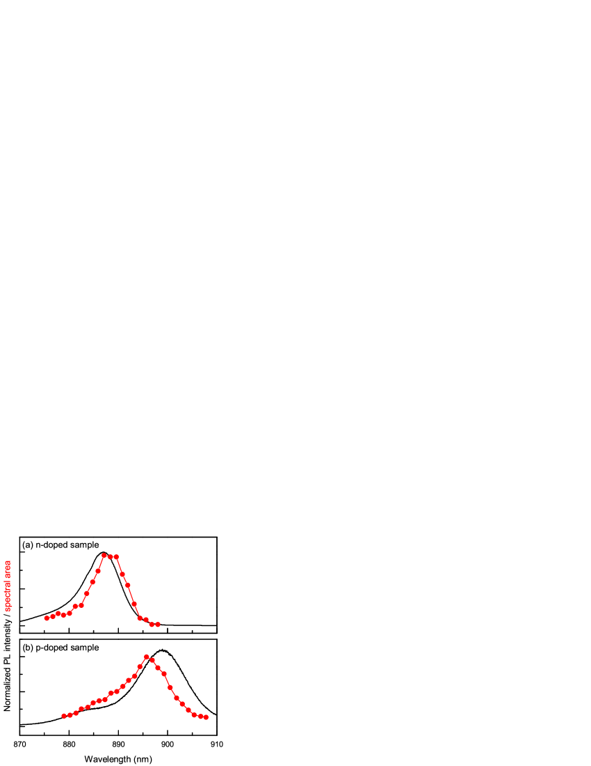
Figure 1: (a) Low excitation PL and spin noise power, i.e. area under the SNS, as functions of the probe wavelength for the $n$-doped QD sample; (b) the same for the $p$-doped sample. The slight red shift of the spin noise compared to the PL for the n-doped sample may result from a concentration of singly charged dots on the low energy side, while towards higher energies the dots become increasingly uncharged. The blue shift in case of the p-doped sample, on the other hand, may result from a double charging of the low energy dots with a pair of holes forming a spin zero singlet state. Towards the high energy side single resident hole spin charging occurs in the dots, resulting in an increase of spin noise. This increased p-doping level is confirmed by the increased intensity of emission from excited states compared to the n-doped sample.

The linearly polarized probe light is taken from a tunable continuous wave (cw) Titanium-Sapphire ring laser emitting a single frequency laser line with a linewidth of < 10 MHz. The laser is then guided through a single mode optical fiber for spatial mode shaping ($\text{TEM}_{00}$). After a Glan-Taylor polarizer providing a linear extinction ratio of 10⁵, the beam is transmitted through the sample with a large area focus of 100 micrometers diameter, in order to minimize optical excitation effects in the QD ensemble yl2012 ; sp1 .

Detection of the Faraday rotation noise is done with a standard polarimeter, consisting of a Wollaston prism and a broadband optical balanced detector. Two different detectors are used to study slower and faster dynamics: one has a bandwidth of 40 kHz $\div$ 650 MHz (New Focus 1607-AC) requiring optical powers of typically a few milliwatts (fast detector), while the other one (Femto HCA-S) covers a bandwidth of DC $\div$ 100 MHz, requiring powers of a few hundreds of microwatts (slow detector). The output of the detectors is amplified and low-pass filtered at variable cutoff frequencies to avoid undersampling, and then sent to the input of a digitizer. The digitizer incorporates field programmable gate array (FPGA) technology for real time computation of the Fast Fourier Transform (FFT) of the digitized voltage samples. The maximum bandwidth is limited at 1 GHz, providing 16384 spectral lines at a spectral resolution of 61.04 kHz. If necessary, the bandwidth can be reduced down to 200 MHz with a resolution of 12.21 kHz. For even higher resolution as required, e.g., in the case of zero and longitudinal magnetic field measurements, spectra could be also acquired with a PCIe digitizer card installed in a computer, in combination with multicore FFT processing and averaging. In this work, the signal accumulation times varied between 1 minute and 30 minutes, depending on the overall noise signal amplitude.

Figure 1 shows, in addition to the PL spectra discussed above, the integrated spin noise power, i.e. the area under the spin noise power density spectrum (SNS), $\int_{0}^{\infty}d\omega(\vartheta_{F}^{2})_{\omega}$, as function of the probe wavelength for both samples. The spin noise power nearly follows the PL line, with maxima at 889 nm for the $n$-type sample and at 896 nm for the $p$-type sample. This is the typical behaviour for inhomogeneously broadened ensembles vz2013 . Thus the laser is tuned into the absorption band to provide measurable noise signal.

Using electromagnets we are able to apply magnetic fields, in the longitudinal direction (Faraday geometry, along the growth direction of the sample) up to $B_{z,max}$ = 120 mT and in the transverse direction (Voigt geometry) up to $B_{x,max}$ = 350 mT. In order to remove the spin-independent contribution to $(\vartheta_{F}^{2})_{\omega}$ from the overall photon shot noise and the intrinsic electronic noise, the spin noise measurements were interleaved between two magnetic fields: one measurement with the desired strength and direction, and the other one applied in the Voigt geometry at $B_{x}\geqslant$ 250 mT for shifting the precession peak out of the detectable bandwidth. Subtraction of both spectra then yields the pure spin noise contribution. In order to account for the frequency dependent sensitivity of the detectors, the noise power spectra were additionally normalized by the photon shot noise power spectra measured without the sample, with the laser radiation shone directly onto the detectors.

IV Results and Discussions

In this section we present the experimental data for the spin noise measurements in zero and finite transversal or longitudinal magnetic fields. Furthermore we provide the results of the simulations using the two theoretical approaches and discuss their limitations and advantages.

Note that for convenient comparison with the experiment we present characteristic frequencies of the two models, such as $\delta_{e}$ and $\delta_{h}$, as well as Larmor frequencies and simulated spin noise spectra, in units of MHz, i.e. in units of an ordinary frequency, rather than by an angular frequency as used in the models.

IV.1 Spin noise at zero magnetic field

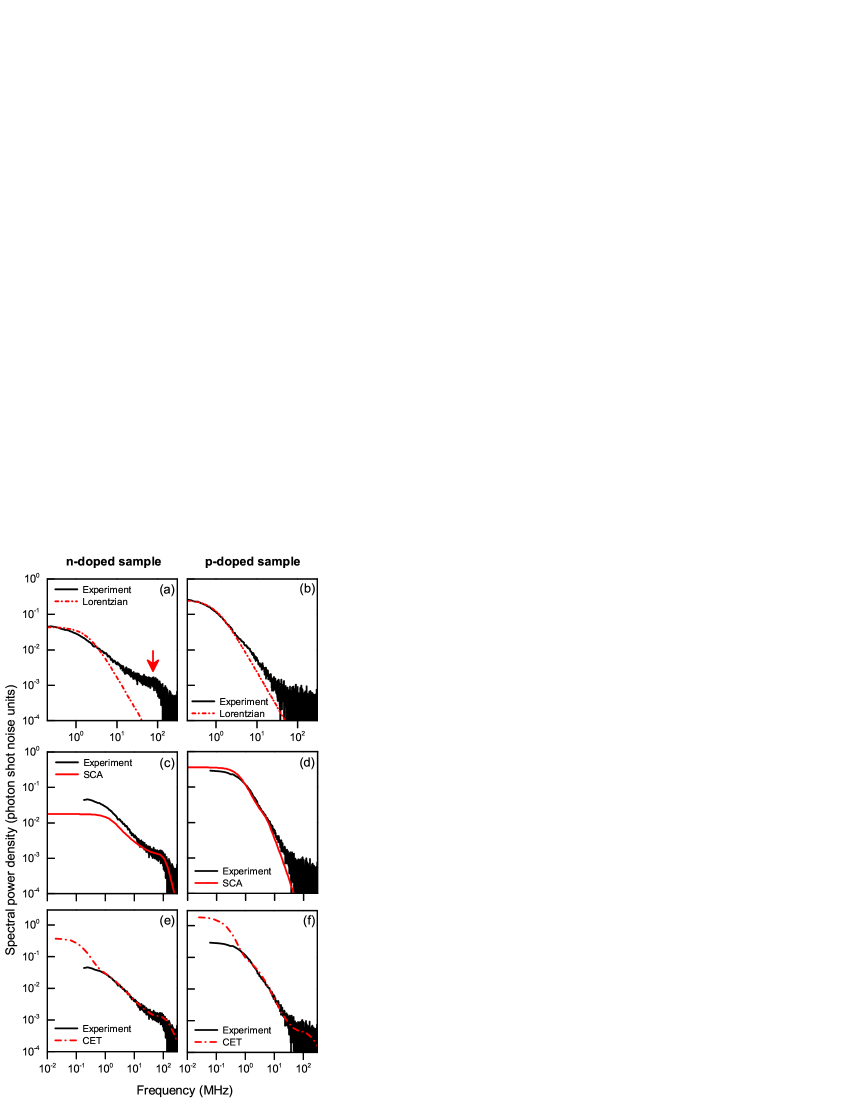
Figure 2: SNS measured on the (a) $n$-doped and the (b) $p$-doped QD samples at zero external magnetic field using a probe power of 4 mW (50 W/cm²) with the fast detector. The red arrow in panel (a) indicates the feature related with the precession of electron spins due to the hyperfine coupling to the nuclei. Panels (c) and (d) show additionally fits (red curve) to the experimental data with the semiclassical model using the parameters $\delta_{e}=70$ MHz, $\tau_{s}^{e}=5$ ns, $\delta_{h}=40$ MHz, $\lambda_{h}=10$, $\tau_{s}^{h}=80$ ns (c) and $\tau_{s}^{h}=240$ ns (d). The spectra are calculated using Eqs. (2) and (11) with $\mathcal{A}N_{e}/(\mathcal{B}N_{h})=4$ for panel (c), and Eq. (11) for (d). The dash-dotted red curves in panels (e) and (f) indicate fits obtained with the CET. The CET results are calculated assuming $\lambda_{h}=5$, $\delta_{e}=$ 110 MHz and $\delta_{h}=$ 16 MHz. The electron fraction for the $n$-doped sample is set to $80\,\%$, and to $15\,\%$ for the $p$-doped sample. For the ensemble averaging a Gaussian distribution of the QD radius $L_{0}$ with a relative standard deviation $\Delta L_{0}/L_{0}=0.2$ is assumed. The ratio $Q_{r}$ is set to $0.6$ for electrons and to $6$ for holes since $A^{e}_{k}\approx 10A_{k}^{h}$. All further parameters are chosen as discussed in section II.2.

Figure 2 compares the spin noise spectra for $n$- and $p$-doped QDs, left and right column of panels, respectively, measured at zero external magnetic field. For these experiments we used the fast detector and the FPGA module to cover a broad frequency range.

As shown in Fig. 2(b), the spin noise in the $p$-doped sample consists of a single peak centered around zero frequency. In the chosen log-log scale representation we find that the curve closely follows a Lorentzian in the frequency domain (shown additionally by the dash-dotted line), which corresponds to an exponential decay in time yl2012 . The spin noise spectrum of the $n$-doped sample reveals, in addition to the zero-frequency peak, a pronounced “shoulder” (termed in the following as precession peak or Overhauser peak) at a frequency of $\sim 100$ MHz, as highlighted by the red arrow in Fig. 2(a). This peak is related to the magnetic field caused by the intrinsic nuclear fluctuations, that act on the electrons as a constant (frozen) magnetic field pointing along a random direction. The electron spin components parallel to the frozen nuclear field contribute to the zero-frequency peak in the signal with $1/3$ of the full spin polarization. The other $2/3$ precess around the nuclear field and are thus seen as the precession peak glazov:review . The absence of such a shoulder in the hole spin ensemble signal is a direct indication of the anisotropic nature of the hole-nuclear interaction mg2012 .

The relative amplitude of the precession peak and the zero-frequency peak is influenced by several factors: (i) finite correlation time of the electron in a quantum dot which might be caused, i.e., by the probe-assisted transfer of the electrons into other QDs, providing a redistribution of the spin noise power of the precession peak towards the zero-frequency peak Glazov_hopping , or (ii) presence of positively charged QDs in the nominally $n$-doped sample, which would increase the relative weight of the zero-frequency peak. In particular, the latter can be tested by applying a transverse magnetic field, as will be shown in the Sec. IV.3. It should be foreclosed at this point, that by applying this method we were able to evidence a percentage of about 20 $\%$ of such non-intentionally $p$-doped QDs, which is mostly due to impurities in the MBE machine. However, this value slightly varies with the point at which the sample is probed by the laser. Thus, to reproduce the data in the semiclassical model, we assume that the ratio of electron and hole contributions to the measured SNS is $\mathcal{A}N_{e}/(\mathcal{B}N_{h})=4$, see Eq. (2). The corresponding fit results for the $n$-doped sample are presented in Fig. 2(c), from which we can determine $\delta_{e}\approx 70$ MHz and $\tau_{s}^{e}=5$ ns, which is consistent with estimations based on the hyperfine coupling constants, Eq. 10. For the hole fraction in the same sample best agreement was achieved with $\delta_{h}=40$ MHz, $\lambda_{h}=10$ and $\tau_{s}^{h}=80$ ns.

The best agreement with the experimental data using the semiclassical model for the $p$-doped sample, see the red curve in Fig. 2(d), is obtained by using the parameters $\delta_{h}=40$ MHz and $\lambda_{h}=10$ in Eq. (5), as well as $\tau_{s}^{h}=240$ ns in Eq. (11) (note that the curve is practically insensitive to a particular value of $\delta_{h}$ provided that $\delta_{h}/\lambda_{h}<5$ MHz)

The panels (e) and (f) of Fig. 2 show a direct comparison between the experimental data and the numerical results obtained via the CET approach. The spin noise function obtained via the CET is highly sensitive to the choice of the model parameters introduced in Sec. II.2. For electron spins, panel (e), the agreement between theory and experiment in the numerically accessible regime is excellent. The pronounced deviation at small frequencies stems from the finite frequency resolution of the CET above $0.79\,\text{MHz}$ for the parameters used here.

The agreement between theory and experiment is less striking for the hole doped sample, where the theoretically determined gradient of the spin noise function in the intermediate frequency regime $0.79\,\text{MHz}<\nu<6\,\text{MHz}$ does not reproduce the experiment exactly. We attribute that discrepancy to the small amount of nuclei in the CET simulations limiting the low frequency spectrum of the Hamiltonian (3). The obtained agreement between experiment and theory is still remarkably good within the finite size limitations of the CET and states the validity of the applied model. All important parameters obtained from describing the experimental data using the two models are summarized in Table 1.

Table 1: SCA and CET parameters determined from the zero magnetic field data which are consistently used also subsequently in describing the data in magnetic field.

	SCA	CET
$\delta_{e}$ (MHz)	70	110
$\delta_{h}$ (MHz)	40	16
$\lambda_{h}$	10	5

IV.2 Long-time spin dephasing at zero field

As a nearly non-perturbative method of measurement, spin noise should be able to unveil the intrinsic spin lifetimes in the studied systems. However, the inhomogeneously broadened QD ensembles require the probe energy to be within the PL-emission band. Therefore, one has to pay special attention to the applied laser power and use the limit of lowest possible laser intensities to minimize excitation effects. As could be shown by Yan Li et al. for hole spins in a very similar sample, for the used large 100 $\mu$m laser spot and used probe powers in the range of 0.1 mW, the QD spin noise shows only a weakly increasing linewidth of the zero-frequency peak with increasing probe power yl2012 ; sp1 . This shows, that probe induced effects are still present, but are minimized. A linear fit of the linewidth power dependence should thus allow us to obtain a rather accurate value of the intrinsic spin relaxation time by extrapolating the fit to zero probe power. This method was recently proven to give reliable results for the electron spin relaxation times in pump-probe studies prb2015_on_T1 .

In our experiments, the zero-frequency peak in the spin noise of the $n$- and $p$-doped sample is measured using the slow 100 MHz detector. Its output is filtered for the frequency band from 0.01 MHz to 32 MHz and then sent through a high frequency amplifier. The probe laser powers range from 0.1 mW to 0.6 mW. Since especially the lineshape of the SNS from the $n$-doped QDs deviates from Lorentzian (see above), we use a general definition of the linewidth, namely the geometrical half width at half maximum (HWHM) of the zero-frequency peak spectrum, denoted as $\Gamma$, see also Ref. yl2012 .

The effective linewidths extracted from our experimental data are depicted in Fig. 3. We observe a weak increase of the linewidths with laser power in both samples. However, the changes are much larger for the $n$-doped QDs. This partly originates from the much smaller spectral amplitudes of the zero-frequency peak as compared to the $p$-doped QDs, for which the complete spin noise power is concentrated in the zero-frequency peak.

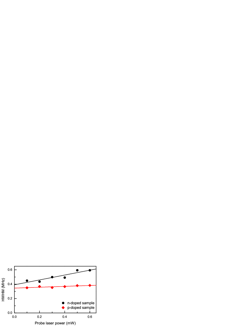
Figure 3: Dependence of the HWHM of the zero-frequency spin noise peak on probe laser power. The data exhibit a weak linear increase with power in both cases, whereupon for the $n$-doped sample the increase is a factor 2.5 stronger. The larger error is caused by a much smaller spectral amplitude compared to that of the $p$-doped sample. We determine the effective intrinsic spin lifetime in both samples by using the point of intersection of the linear fits with the vertical axis at zero laser power.

From linear fits to the power dependences we obtain the following intrinsic linewidths: the $p$-doped sample obeys $\Gamma=(0.35\pm 0.01)$ MHz, whereas $\Gamma=(0.39\pm 0.03)$ MHz for the $n$-doped sample. The linear increase of the linewidth is steeper for the n-doped dots: it grows by $40\%$ as the probe power is increased from 0.1 mW to 0.6 mW. For hole spins we observe an increase of only $10\%$ within the same range of laser power. This difference shall be studied in greater detail in future, here we point out only some related aspects. First, as has been already mentioned above, there is a finite fraction of $p$-doped QDs in the intentionally $n$-doped sample, which amounts to about 20 %. Since at zero external field $2/3$ of the electron spin noise is concentrated in the precession peak and only $1/3$ contributes to the zero-frequency peak, holes then may contribute up to 40 % to the spin noise of the zero-frequency peak, while the remaining 60 % stems from electrons. Thus, there is a significant hole contribution that may influence spectral shape and amplitude of the low-frequency SNS from the $n$-doped sample. Second, both samples are measured under exactly the same probing conditions, especially with the same large laser spot of 100 $\mu$m that evidently produces only a weak perturbation of the spin system. We prove this assumption by additionally looking at the FR noise amplitude, which is the square root of the FR noise power, obtained by integration of the SNS from 0.012 MHz to 32 MHz. Taking the dependence of the FR noise amplitude on the probe laser power, we obtain an exponent of $\approx 0.85$ for both samples by fitting the dependence with a power law. This value is quite close to unity, suggesting that the measurements were carried out close to thermal equilibrium, i.e., close to the non-perturbative regime sp1 . As an example of the opposite case, Ref. rd2012 showes signatures of strong optical perturbation, demonstrating the hole spin noise in a QD microcavity with the measurements carried out using $10^{3}\div 10^{4}$ times larger probe intensity than in our case. The linewidth then is increased by a factor of 3, i.e. by 200 % under a threefold increase of laser power. This additionally corroborates that our measurements are performed largely non-perturbatively.

Using the well-known relation $\tau_{s}=(2\pi\Gamma)^{-1}$ we derive the effective spin lifetimes. We obtain $\tau_{s}^{p}$ = 0.46 $\mu$s for the $p$-doped sample, and $\tau_{s}^{n}$ = 0.41 $\mu$s for the $n$-doped sample. These values are close to the known result of $\tau_{s}^{h}$ = 0.4 $\mu$s that was obtained in the Refs. yl2012 ; sp1 . At first glance it is quite surprising that electrons and holes have similar relaxation times, as they show a strong difference in the nuclear interaction strength. Otherwise, similar values for the spin decoherence time $T_{2}$ of QD electron and hole spins in magnetic field were revealed by the mode-locking technique applied to similar $n$- and $p$-doped heterostructures prb87Varwig . As we will explain in the following, our observation of comparable timescales is related to the presence of additional quadrupolar interactions of the nuclei with electric field gradients in the dots, Eq. (6).

Without ${\cal H}_{N}^{\mu}$, the characteristic time scale for the electron spin noise is given by $T^{*}_{e}\propto 1/\delta_{e}$, and the one for hole spins by $T^{*}_{h}\propto\lambda_{h}/\delta_{h}$ determined by the fluctuations of the Overhauser field (10). While $T^{*}_{e}\approx 1-2$ ns is found in the typical QD ensembles as investigated here, the $p$-wave nature of the hole-wave function reduces the hyperfine couplings $A_{k}^{h}$ by a factor of 10 compared to the electron spins Fermi1930 ; Fischer2008 ; testelin . The decay of $S_{h,z}$ is additionally suppressed by the anisotropy parameter $\lambda_{h}\approx 10$, accounting for the anisotropic dipole-dipole coupling of hole spins to the nuclear spins Fermi1930 ; Fischer2008 ; testelin , so that $T^{*}_{h}\approx 100T^{*}_{e}$.

Including a realistic modeling bulutay of the coupling between the nuclei’s quadrupole moments and the electric field gradients (EFGs) in the QDs via ${\cal H}_{N}^{\mu}$ is sufficient to explain the observed mismatch between the experiments and the prediction of the CSM, see also Ref. jh2015 . This can be intuitively understood: adding an additional source of decoherence (i.e. the quadrupole interaction) to the CSM Hamiltonian results in a decrease of the coherence time of the considered electron/hole spins.

Without ${\cal H}_{N}^{\mu}$, the total spin component in $z$-direction,

$$\hat{J}_{z}^{\rm tot} = \hat{S}_{\mu,z}+\sum_{k}\hat{I}_{z}^{(k)},$$ (13)

is a conserved operator in the CSM provided that $\bm{\Omega}_{B}^{{\mu}}=0$ or $\bm{\Omega}_{B}^{{\mu}}\parallel z$, implying that each individual nucleus maintains its state until the next spin-flip process occurs, always involving a combined carrier and nuclear spin flip.

Adding ${\cal H}_{N}^{\mu}$ breaks this conservation law for $\hat{J}_{z}^{\rm tot}$ in the CSM by allowing spin-flips in the nuclear spin bath without involving the electronic spin, and defines an additional long-time scale set by the coupling strength ${\cal H}_{N}^{\mu}$. Its effect onto the spin-noise function can be investigated in fourth order perturbation theory HackmannPhD2015 for fixed nuclear easy-axis vectors $\vec{n}^{(k)}_{z}=\vec{e}_{z}$: a term linear in $q_{k}$ and cubic in $A_{k}^{\mu}$ accelerates the decay of $S_{\mu,z}$ but a $q_{k}^{2}$ term decelerates the spin decay. We note that the influence of ${\cal H}_{N}^{\mu}$ onto the decay of the electronic spin is indirect and only occurs in combination with the hyperfine interaction. Its effect is non-universal and cannot be casted into a simple decay time or energy scale as defined by the fluctuation of the Overhauser field (10). The reason is related to its two opposite limits. For $A_{k}>q_{k}$, typically relevant for the experiment, ${\cal H}_{N}^{\mu}$ provides additional nuclear spin-flip processes leading to an additional spin decay at long time scales set by $Q_{r}$, Eq. (12), as outlined above. For the opposite limit, $A_{k}\ll q_{k}$, the nuclear system must be diagonalized first, providing a set of two time-reversal doublets as the new eigenbasis for each nuclear spin energetically separated by $2q_{k}\sqrt{1+\eta^{2}4/3}$. Then the coupling to the electron/hole spin is treated perturbatively, and the rigidity of the nuclear system can suppress additional dephasing for $\eta\to 0$ HackmannPhD2015 ; Wu2015 .

Since the $\vec{n}^{(k)}_{z}$ have different strain induced orientations at each nuclei in a real QD, their angular distribution bulutay and the in-plane anisotropy $\eta$, however, provide an additional source of randomness and, hence, spin dephasing even for stronger hyperfine coupling due to the misalignment of the local nuclear easy-axis and the growth orientation, defining the global $z$-axis.

Crucial for the understanding of the comparable long-time spin decay of electron spins and hole spins is the fact that ${\cal H}_{N}^{\mu}$ is caused by the growth induced strain in the QDs, and its energy scale is consequently independent of the QD doping. This additional source of decoherence counteracts the lifetime enhancement of a factor $10\lambda_{h}$ as predicted within the CSM for hole spins. The quantum mechanical CET predicts jh2015 that the long-term lifetime is of the same order of magnitude for $n$-type and $p$-type QDs grown under identical growth conditions, as demonstrated in Fig. 2(e) and (f).

At values $Q_{r}\approx 6$ as used in Fig. 2(f), the nuclear quadrupole electric couplings become the limiting factor of the coherence time in zero magnetic field.

On a semiclassical level, the influence of the additional quadrupolar couplings can be understood by investigating the equation of motion of a single nuclear spin in the Hamiltonian (3) coupled to a fictitious static carrier spin. Within the CSM only, the nuclear spin would precess around this central spin with a Larmor frequency proportional to the individual $A_{k}^{\mu}$. This leads to slow dynamics of the Overhauser field merkulov02 and a long-time carrier spin decay described by a power law CoishLoss2004 ; jh2014-1 with some logarithmic corrections governing the low frequency part of the spin-noise spectra. Adding the quadrupolar couplings ${\cal H}_{N}^{\mu}$ has two effects on the nuclear spin dynamics: firstly it enhances the nuclear Larmor frequency, and, secondly, the breaking of the total spin conservation law translates into a change of an effective precession axis which is not longer determined by the carrier spin direction only. Both effects yields to an addition dephasing of the Overhauser field and consequently to a dephasing of the non-decaying fraction of the spin-correlation function uhrig2014 on a time scale dominated by the quadrupolar coupling strength.

IV.3 Spin noise in transverse magnetic fields

A magnetic field applied perpendicular to the probe beam propagation direction, $\bm{B}\parallel x$ (Voigt geometry), induces spin precession and shifts the corresponding noise peak along the frequency axis to the Larmor frequency $\Omega_{B}^{\mu}$. We have carried out measurements for electron and hole spins up to field strengths of $B_{x}=80$ mT, using the fast 650 MHz photodetector with a probe power of 4 mW. The experimental results are presented in Fig. 4 panel (a) for the $p$-type sample and panel (b) for the $n$-type sample.

We start the analysis with the data on the $p$-type sample, shown in panel (a). At $B_{x}\neq 0$ the SNS consists of two peaks: the first one remains centered at $\omega=0$, but its amplitude decreases with increasing magnetic field, and the second one appears at $\omega\neq 0$, shifting with the field towards higher frequencies, in agreement with our expectations, see Sec. II.1, because the transverse magnetic field suppresses the role of the nuclear field fluctuations, therefore reducing the zero-peak contribution. The experimental data are adequately described by the semiclassical model, Eq. (11), using the following values of fit parameters: transverse hole $g$-factor $g_{h}^{\perp}=0.16$, measured from the linear shift of the second peak maximum with magnetic field, $g$-factor spread of $\approx 37$ %, measured from the broadening of the peak, and $\tau_{s}^{h}\approx 16$ ns for $B_{x}\geqslant 20$ mT, see the solid curves in Fig. 4(a) for results. To achieve better agreement between experiment and theory at $B_{x}=0$ the curve centered at zero frequency is calculated with a longer spin relaxation $\tau_{s}^{h,0}\approx 240$ ns. This extension of the spin relaxation time by the magnetic field is beyond the scope of the semiclassical model and demonstrates its limitations.

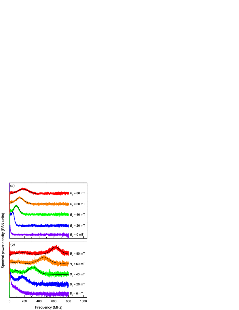
Figure 4: (a) SNS measured on the $p$-doped QD sample in the transverse magnetic fields indicated in the legend. The acronym "PSN" means "photon shot noise". Fits with the semiclassical model are shown by the solid lines at $B_{x}$ = 40 mT and 80 mT. The heavy hole $g$-factor is $g_{h}^{\perp}=0.16$ with a spread of 37%. Other parameters of calculations are the same as for Fig. 2(d) except for $\tau_{s}^{h}=16$ ns at $B_{x}\geq 20$ mT. The dashed line at $B_{x}$ = 60 mT indicates a fit with the CET model, for which a Gaussian hole $g$-factor spread with a relative standard deviation of $\Delta g/g=0.15$ has been assumed; (b) SNS measured in the $n$-doped QD sample at the same transverse magnetic fields, showing also signatures of hole doped QDs in the ensmble. Fits with the semiclassical model are again depicted by solid lines, with parameters of the hole spin noise being the same as in panel (a). Electron $g$-factor is $g_{e}^{\perp}=0.55$ with a spread of 7% and the other parameters are the same as for Fig. 2(c). The fit at $B_{x}$ = 60 mT uses again the CET approach, with the $g$-factor being the same as for the SCA approach. All other CET parameters except the hole $g$-factor spread are the same as in Fig. 2.

To illustrate further the validity of the semiclassical model at non-zero fields and to analyze the interplay of the nuclear spin fluctuations and the external magnetic field in more detail, we plot the ratio of the area under the zero-frequency SNS peak to the area under the whole SNS for an extended range of field strengths up to $B_{x}$ = 120 mT, see Fig. 5. The area of the zero-frequency peak was extracted by fitting the SNS by a linear combination of a Gaussian function centered at $\omega\neq 0$ and two Lorentzians centered at $\omega=0$ with different widths. The Gaussian function is needed to account for the non-zero frequency spin precession peak and the two Lorentzians reflecting exponential decays in time are needed to reproduce rather accurately the shape of the zero-frequency component whose precise calculation is beyond the scope of the semiclassical model. The Gaussian is characteristic for a behavior determined by an inhomogeneous distribution such as the $g$-factor variations mg2012 . Figure 5 demonstrates good agreement between theory and experiment.

Next we turn to the SNS of the $n$-type QD sample in transverse magnetic field, shown in Fig. 4(b). Here, at $B_{x}\neq 0$ one can see two features in the SNS appearing at non-zero frequencies. One of them correlates with the hole Larmor precession, Fig. 4(a), while the other one has much higher frequency and can be attributed to the electrons. As mentioned above, the ratio of the areas under these two peaks is slightly sensitive to the particular point of the sample that is probed by the laser.

This observation supports our conjecture that $n$- and $p$-doped quantum dots coexist in the nominally $n$-type sample, see Sec. IV.1. Hence, as in Sec. IV.1, to describe the experimental data within the semiclassical model we take into account contributions of electron and hole spins to the measured SNS. The particular data in Fig. 4(b) are well described by Eqs. (2) and (11), see solid curves in Fig. 4(b), calculated using a fraction of positively charged QDs, $\mathcal{A}N_{e}/(\mathcal{B}N_{h})\approx 4$. Other fit parameters are chosen as follows: $g_{e}^{\perp}=0.55$, its spread is about $7$ %, and $\tau_{s}^{e}=5$ ns, taken independent on $B_{x}$. We note that such a short value of $\tau_{s}^{e}$ is introduced into the semiclassical model to approximate the relatively broad zero-frequency contribution in the SNS. An analysis of the “intrinsic” electron spin relaxation time is presented below in Sec. IV.4.

In Fig. 4 we demonstrate the agreement between the experimental results and the CET for transversal external fields. The CET parameters are set to those of the zero-field calculation used in Fig. 2. The comparison between the experimental results and the CET data (dashed lines) for $B=60\,\text{mT}$ serves as a proof of principle assuring comparable results for the remainder experimental data. For the $p$-type samples, the electron-spin contribution to the spectrum is negligible, and the CET reproduces the obtained hole-spin spectrum at all frequency ranges in Fig. 4(a).

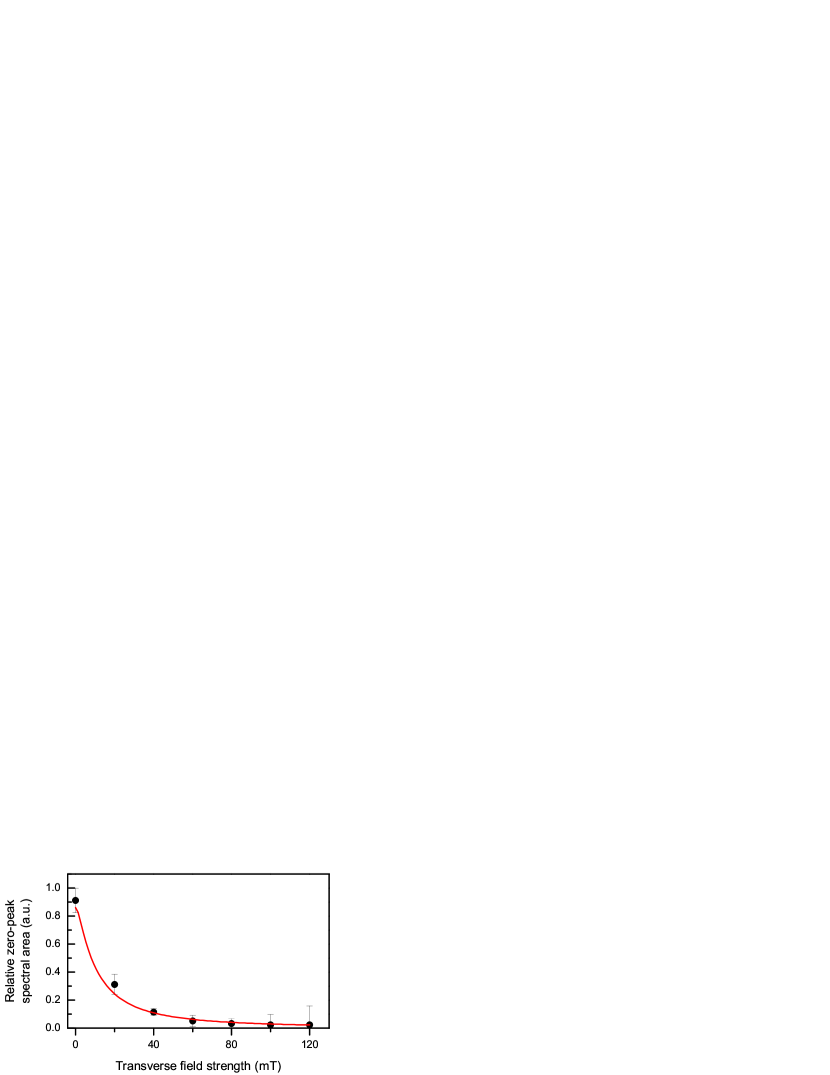
Figure 5: Analysis of the relative spectral area of the zero-frequency peak as a function of transverse magnetic field calculated for the $p$-doped sample using the semiclassical approach. Points are obtained by fitting the experimental data, see text for details. The solid curve is calculated using Eq. (11) with the same set of parameters as Fig. 4(a).

As noted above, the SNS of $n$-type samples shows a shallow low-frequency feature tracing perfectly the spin-noise peak of the $p$-type samples with increasing magnetic field. Due to the $\sim 20\,\%$ admixture of holes to the $n$-doped spectrum, the hole SNS provides an additional finite low-frequency contribution around the hole Larmor frequency that is accurately reproduced by the CET approach as shown in Fig. 4(b). As previously demonstrated mg2012 ; jh2014-1 , the width of the spin precession peak is mainly governed by the parameter $\delta_{\mu}$ at small and moderate fields, while at higher fields it is controlled additionally by the $g$-factor spread; the peak shape is approximately Gaussian for $\Omega_{B}\gg\delta_{\mu}$.

The transversal magnetic field reduces the non-decaying fraction of the spin-correlation function responsible for the zero-frequency $\delta$-peak in the spin-noise spectrum. Consequently spectral weight is transferred to finite frequencies to fulfil the spectral sum rule mg2012 ; jh2014-1 ; oest:nsn , which describes the conservation of a total number of fluctuating spins. This is clearly visible in the $p$-type spectra shown in Fig. 4(a). Such a suppression is also found in $n$-type samples.

Synopsis of the transverse-field results shows that the data in Figs. 4 and 5 can be well described by both models, the semiclassical and the quantum-mechanical one.

IV.4 Spin noise in longitudinal magnetic fields

Under application of a magnetic field along the light propagation axis the role of transverse fluctuations of the Overhauser field diminishes. This leads to: (i) suppression of the precession peak, and (ii) modification of the zero-frequency peak amplitude and shape. As noted above, the total area under the noise spectrum remains constant and does not depend on magnetic field due to conservation of the number of spins in the probed volume.

In this section we focus on the zero-frequency peak. This allows/requires (i) usage of the highly sensitive slow detector with low probe laser powers to minimize optical excitation effects and (ii) detailed monitoring of zero-frequency peak modifications because of higher spectral resolution. In particular, we filtered the detector output voltage for the frequency band between 0.009 MHz and 17.5 MHz.

The suppression of the precession peak in the $n$-doped sample then becomes indirectly observable by changes of the integral spectral area of the zero-frequency peak, as for higher longitudinal fields the spins become stabilized and redistributed in frequency into the zero-peak component.

Figure 6 shows the low-frequency SNS of the $n$-type sample, panel (a), and of the $p$-type sample, panel (b), measured at 0.2 mW probe laser power for different values of the longitudinal magnetic field. It was our aim to measure both samples under comparable probing conditions with the lowest possible laser power. The chosen low probe laser power is dictated by the small noise amplitude in the selected frequency range for the $n$-doped sample at zero external field, because the nuclear field distributes 2/3 of the total spectral weight of the electron spin noise into the Overhauser precession peak (not shown).

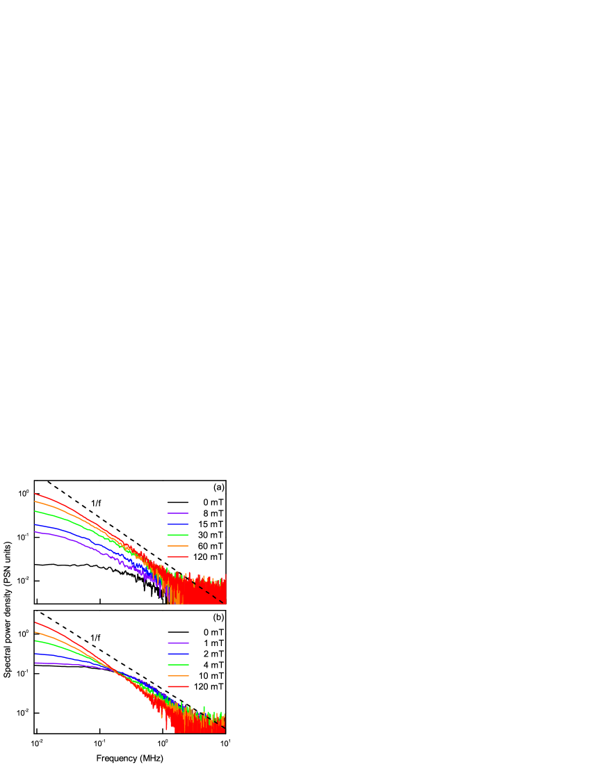
Figure 6: SNS measured on the (a) $n$-doped and (b) $p$-doped QD ensemble at different longitudinal magnetic fields using a probe laser power of 0.2 mW, see legend for the field strengths. The black dashed lines illustrate the $1/f$-asymptotics.

The experimental data clearly demonstrate the enhancement of the zero-frequency peak with increasing magnetic field. The spectra of both samples transform towards a $1/f$ behaviour of the SNS at sufficiently high field strengths, as reported previously for a $p$-doped sample yl2012 . This indicates a crossover to a $1/\ln{t}$ spin decay in time, which is especially noteworthy for the $n$-doped sample, since the longitudinal field redistributes electron spin fluctuations from the Overhauser precession peak into the zero-frequency peak (see below), such that at the maximum applied field strength the electron spin contribution to the zero-frequency peak clearly dominates, despite the finite admixture from $p$-doped QDs. Thus, the crossover to $1/f$-noise can be termed a general property of carrier spins in QDs, regardless of the type of resident carrier charge.

To obtain deeper insight into the complex dynamics of interacting electron and nuclear spins we extract again the effective spin relaxation times $\tau_{s}$ from the half-width at half-maximum (HWHM) of the zero-frequency SNS component, see Fig. 7(a). Since the shape of the zero-frequency feature strongly deviates from a Lorentzian, especially for sufficiently high magnetic fields where $1/f$ behavior dominates, such procedure only gives effective timescales for the spin relaxation, as explained above in Sec. IV.2.

The red dimonds in Fig. 7(a) show the effective relaxation times $\tau_{s}^{p}$ for the $p$-doped QD sample. It abruptly increases with increasing magnetic field up to $\sim 10$ mT, from $\sim 0.4$ $\mu$s (consistent with the measurements shown in Secs. IV.1, IV.3) to 5.3 $\mu$s. The longitudinal field overwhelms the anisotropic nonzero hyperfine field experienced by the hole through the hole-nuclear coupling, and thus suppresses the hole spin dephasing due to hyperfine interaction. For the magnetic field range from 20 mT to 120 mT, $\tau_{s}^{p}$ slowly increases further up to about $6.5$ $\mu$s, showing signatures of saturation at the highest field strengths. We ascribe this behaviour to a small fraction of non-intentionally $n$-doped QDs in this sample. Notably, the width of the dip in the magnetic field dependence of the electron spin lifetime around zero field should be considerably larger than that for holes. This is because the hyperfine field acting on the electron spin is stronger. Hence, a larger external magnetic field is needed to overcome the hyperfine field. This assumption is supported by the spin lifetime behaviour $\tau_{s}^{n}(B_{z})$ observed for the $n$-doped sample, see black dots in Fig. 7(a). The broad component is significantly more pronounced than in the $p$-doped sample. The narrow dip for fields $|B_{z}|\lesssim 10$ mT is ascribed to the presence of $p$-doped QDs in the $n$-type sample. The broad, electron-induced component demonstrates a further increase in the effective electron spin lifetime to 5.6 $\mu$s, showing also pronounced signatures of saturation at $|B_{z}|=120$ mT.

Additionally, with increasing magnetic field strength, the 2/3 of total spectral weight of electron spin noise contained at zero external field in the precession peak become continuously redistributed into the zero-frequency peak. In order to demonstrate this behaviour, we made use of two facts: (i) a simple measure for the spectral weight of the spin noise is provided by the area under the SNS, which in turn can be obtained from an integration, $\int_{\omega_{1}}^{\omega_{2}}d\omega\left(\vartheta_{F}^{2}\right)_{\omega}$; (ii) for the analysis of the redistribution, it is sufficient to monitor the increase of the spectral area under the zero-frequency peak. Thus, we performed the integration of the SNS in the frequency range depcited in Fig. 6, i.e. from 0.009 MHz to 10 MHz.

For our $n$-doped sample we finally obtain a dependence of the zero-frequency peak area on $B_{z}$ as depicted by the black dots in Fig. 7(b). The continuous redistribution of the spectral weight of the electron spin noise is clearly seen, whereupon saturation occurs for $|B_{z}|\geqslant$ 80 mT. In principle, the observed behaviour can be explained with the total longitudinal field overcoming the transverse components of the nuclear hyperfine field that is isotropic in the n-doped QD ensemble, such that finally an anisotropic total magnetic field acts on these QDs, shuffling all spectral weight of the electron spin noise into the zero-frequency peak, as is the case for hole spins mg2012 . However, the total increase of the zero-frequency peak area in the $n$-doped sample amounts to a factor of $\sim$2.3 only, instead of the expected factor of $3$ mg2012 . This is in line with the presence of $p$-doped QDs, and the spectral cutoff at the smallest frequencies ($f<0.009$ MHz).

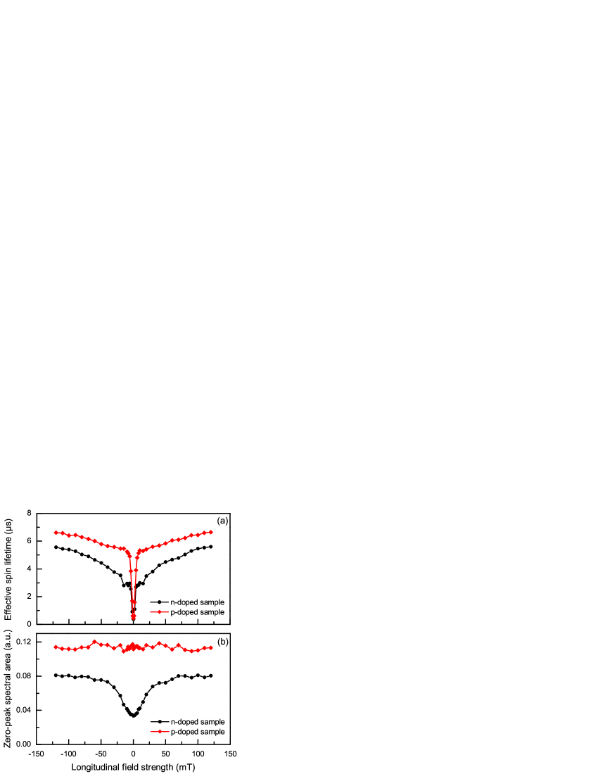
Figure 7: Dependence of (a) the effective spin lifetime inferred from the HWHM of the zero-frequency peak SNS, and (b) the area under the zero-frequency peak SNS of both QD samples on longitudinal field strength. Each sample shows some characteristic features of a fraction of QDs in each ensemble being doped non-intentionally with the other type of carrier spin, respectively. This is due to impurities incorporated during the growth process.

To complete the discussion of the experimental observations, we address the dependence of the spin noise amplitude of the $p$-doped sample on the longitudinal field strength, see the red diamonds in Fig. 7(b). The absence of any pronounced dependence on $B_{z}$ indicates that the amount of $n$-type quantum dots in this sample is rather small. Indeed, for $\lesssim 10$ % of $n$-type dots their contribution to the zero-frequency peak amplitude can hardly be resolved within our experimental accuracy.

Summarizing the experimental findings, we note that in sufficiently strong magnetic fields (which suppress the frozen nuclear fields) both types of carrier spins (i) demonstrate quite similar effective spin lifetimes, and (ii) show a trend towards a $1/\ln{(t)}$ spin decay manifesting itself as a $1/f$ behavior of the zero-frequency peak SNS.

The semiclassical model outlined in Sec. II.1 provides an increase of $\tau_{s}^{h}$ with increasing longitudinal magnetic field if a finite value of the correlation time $\tau_{c}$ is taken into account. However, our estimations show that such an increase should be observed at larger fields than observed, $B_{z}\sim 20$ mT for the parameters extracted from the fits in Sec. IV.3. Hence, such an abrupt increase as well as the weak increase of the hole spin relaxation time at $\Omega_{B}^{\mu}>\delta_{\mu}$ should be analyzed in terms of the interconnected hole and nuclear spin dynamics yl2012 , quadrupolar splittings sinitsyn:quad and, possibly, taking into account other spin relaxation mechanisms unrelated to the hyperfine interaction Khaetskii1 . On the other hand, the semiclassical model provides a reasonable description of the redistribution of the spectral weight of electron spin noise into the zero-frequency peak under longitudinal magnetic fields: taking the value of $\delta_{e}=70$ MHz from the fitting of the zero-field SNS, Fig. 2(c), as well as 20 % of $p$-doped QDs, $AN_{e}/(\mathcal{B}N_{h})=4$, we obtain the red solid curve in Fig. 8 without any additional fitting parameters, giving fair accord with the measured data. Note, that the value of the electron spin lifetime $\tau_{s}^{e}$ only weakly affects the dependence of the zero-frequency peak area on the longitudinal magnetic field.

Within the CSM, the suppression of the electron spin decoherence in a longitudinal field $\bm{B}\parallel z$ with field strength $B_{z}=|\bm{B}|$ leads to a rapid increase of the long-time limit $S_{\infty}(b)=\lim_{\tau\to\infty}S_{e}(\tau)$ of the spin correlation function $S_{e}(\tau)$ defined in Eq. (7). $S_{\infty}(b)$ is proportional to the spectral weight of the zero-frequency peak contribution, and its dependency on the dimensionless magnetic field $b=\Omega_{B}^{e}T_{e}^{*}$, with $\Omega_{B}^{e}$ denoting the frequency of the Larmor precession induced by the longitudinal field ($\bm{\Omega}_{B}^{e}\parallel z$), is given by the interpolation formula

$$S_{\infty}(b) = S_{e}(0)-\frac{S_{e}(0)-S_{\infty}(b=0)}{1+b^{2}}$$ (14)

for the $n$-type QDs HackmannPhD2015 , with $S_{e}(0)=1/4$ being the initial value of the spin-correlation function (1) at time $t=0$, and $T_{e}^{*}\propto 1/\delta_{e}$ denoting the characteristic timescale of the electron spin fluctuations (see above). Note, that Eq. (14) holds in the SCA as well with an accuracy higher than $4\leavevmode\nobreak\ \%$.

Within the quantum mechanical approach jh2014-1 to the CSM it was found that (i) the spectral weight of the spin precession peak rapidly decays as $\propto b^{2}$ HackmannPhD2015 , (ii) the low-frequency spectral weight ($1/\tau_{s}^{e}\ll\omega\ll\delta_{e}$) is strongly reduced as well as (iii) collapsing into the zero-frequency peak jh2014-1 ; HackmannPhD2015 leading to Eq. (14) for longitudinal magnetic fields.

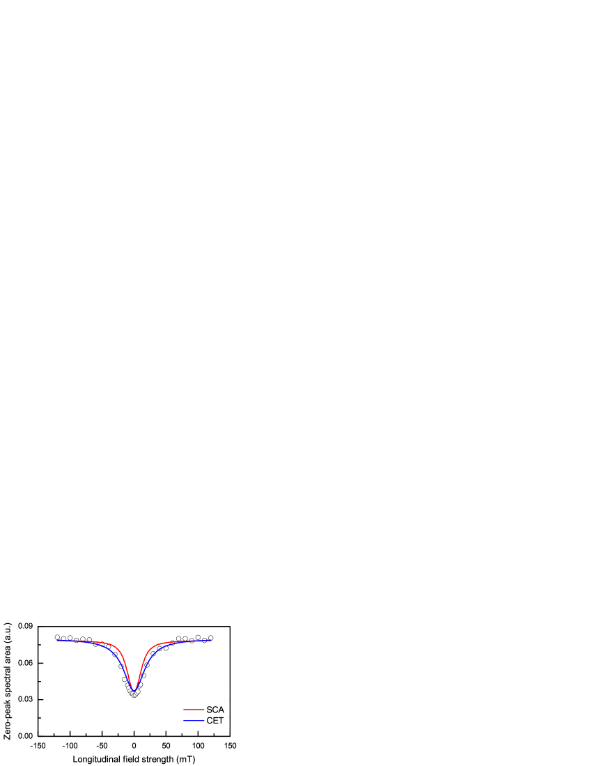
Figure 8: The red line shows a fit to the data shown in Fig. 7(b) using the semiclassical approach with $\delta_{e}=70$ MHz and $AN_{e}/(\mathcal{B}N_{h})=4$ as obtained from the zero-field and transverse-field SNS. The blue line shows $S_{\infty}(b)$ obtained from Eq. (14), under particular consideration of Eq. (15), and with parameters $\delta_{e}$ = 110 MHz and $S_{e}(0)/S_{\infty}(b=0)$ = 2.14 consistent with the CET calculations added to Fig. 2, as well as $S_{e}(0)$ = 0.08.

The SNS shown in Fig. 6 suggests that the high energy parts of the spectrum are not solemnly transferred to the zero-frequency $\delta$-peak as predicted by the CSM, but are distributed over some finite low-frequency range obeying $1/f$ behaviour as shown in Fig. 6. This experimental observation supports the claim that a simple CSM is insufficient to explain the observed SNS, and additional terms in the Hamiltonian are needed for the proper description of low-frequency parts of the SNS.

As mentioned, the $n$-type and $p$-type QDs show similar low-frequency features in the SNS spectrum, leading to the estimated long-time scales in Fig. 7(a) that are quite comparable for both spin species and only weakly field dependent once $\Omega_{B}^{e}T_{e}^{*}\gg 1$. Therefore, the mechanism governing the low-frequency part of the spectrum must be the same for both types of QDs and nearly independent of the longitudinal magnetic field. This serves as a piece of evidence that the nuclear quadrupolar couplings, Eq. (6) and Refs. sinitsyn:quad ; jh2015 provide this mechanism: The quadrupolar splittings defined by the Hamiltonian ${\cal H}_{N}^{\mu}$ are induced during the growth process bulutay and are independent of doping. Moreover, since the nuclear magnetic moment is about 2000 times smaller than the Bohr magneton, the nuclear system remains almost unaffected by the comparably weak longitudinal magnetic fields applied in our experiments.

Replacing the non-decaying fraction of the spin-correlation function uhrig2014 by the integral over the low-frequency part of the spectrum yields the same functional dependence of this signal area on the longitudinal magnetic field as in Eq. (14) for $n$-type QDs. In fact, identifying $S_{\infty}(b)$ with the zero-frequency peak area in the SNS and setting $S_{\infty}(b=0)=S(0)/3$ using the SCA estimate  merkulov02 precisely describes the increase of the zero-frequency peak area as function of the magnetic field, where $S_{e}(0)$ takes the role of a prefactor fixed by the experiment. For the particular case of admixture from non-intentionally $p$-doped QDs as observed in our studies, Eq. (14) should also remain suitable. Then the parameters $S_{\infty}(b=0)$ as well as $S_{e}(0)$ include the same (field-independent) contributions from hole spins, respectively, such that the field-dependent part describes the redistribution of electron spin noise from the Overhauser peak into the zero-frequency peak, regardless of the amount of $p$-doped QDs in the sample.

In order to find out whether the expression in Eq. (14) is sufficient to describe the data depicted in Fig. 7(b) under utilization of the CET parameters derived from the zero-field and transverse-field measurements ($\delta_{e}$ = 110 MHz, $\sim$20 % of hole doped QDs), we firstly derived a relation for the dimensionless magnetic field $b$ that contains both $\delta_{e}$ and $B_{z}$. Therein, we put $\Omega_{B}^{e}=\hbar^{-1}g_{e}^{\parallel}\mu_{B}B_{z}$. Furthermore, by taking $\Omega_{N}^{e}$ to denote the Larmor frequency of the precession peak in the zero-field SNS, we can adopt (i) $\Omega_{N}^{e}\approx\left(\sqrt{2}T_{e}^{*}\right)^{-1}$ as a major CET result jh2014 , and (ii) $\Omega_{N}^{e}=\delta_{e}$ from the SCA mg2012 , to obtain $T_{e}^{*}=\left(\sqrt{2}\delta_{e}\right)^{-1}$. In combination, the relation

$$b=\frac{g_{e}^{\parallel}\mu_{B}}{\hbar\sqrt{2}\delta_{e}}B_{z}$$ (15)

is yielded, which we then included into Eq. (14). Next, we accounted for 20 % of $p$-doped QDs by incorporating the ratio $S_{e}(0)/S_{\infty}(b=0)=2.14$, but left $S_{e}(0)$ as a free parameter to optimize the fit between experiment and theory. Finally, $g_{e}^{\parallel}\approx g_{e}^{\perp}=0.55$ is included. Under all aforementioned preconditions, we obtained the best agreement for $S_{e}(0)=0.08$. The corresponding plot is depicted by the blue curve in Fig. 8. As can be derived from this plot, the CET is well suited to describe our data. Especially, the good consistency of the model parameters obtained previously from the zero-field and the transverse-field measurements deserves particular attention.

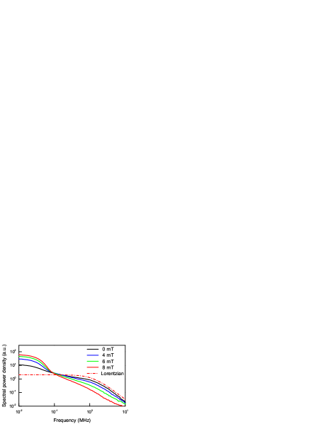
Figure 9: (color online) SNS of a hole doped QD calculated with the CET for $\lambda_{h}=4$ and $Q_{r}=1$ in a varying longitudinal external field $\bm{B}\parallel z$, and for $\delta_{h}=9.7$ MHz. For the $B=0$ spectrum we supplemented a Lorentzian (dash-dotted line) with a half width at half maximum of $\Gamma=1.25\,\text{MHz}$.

With this specific conclusion we turn the analysis to the $p$-type QDs. The situation here is considerably different from the $n$-type QDs: due to the significant anisotropy factor $\lambda_{h}$, the spin decay is suppressed in the CSM: the Gaussian peak from the Overhauser field fluctuation is shifted to lower frequencies approximately by a factor of $10$ testelin compared to $n$-type QDs and, therefore, merges with the rest of the low frequency spectrum, as was also shown in Fig. 11 of Ref. jh2014-1 . In addition, its area is reduced due to the suppression of the spin decay via the hyperfine coupling. To this end, the depicted frequency range in Fig. 6(a) contains almost the complete spin noise, and, consequently, the area remains constant within the experimental restrictions as reported in Fig. 7(b) and in accordance with the spectral sum rule.

For a detailed comparison between the experiment and the CET approach for the full Hamiltonian (3), the frequency resolution for the SNS must be matched. Since we have typically used a fixed number of Chebyshev polynomials $N_{c}=6000$, and the energy spectrum of the Hamiltonian (3) increases with increasing magnetic field, the lowest accessible frequency in the CET approach also increases with the applied magnetic field. Therefore, the CET has very reliable access to the high-frequency part of the spectrum above 1 MHz, while that part on the experimental side is unfortunately already disappearing in the detector noise. On the other hand, the CET approach lacks the necessary low-frequency resolution for $f<$ 1 MHz with increasing longitudinal magnetic field, where the crossover to a $1/f$-type spin decay has been detected in experiment as reported above.

Nevertheless, such a crossover has also been found in a longitudinal magnetic field when applying the CET approach to the full Hamiltonian (3) for $p$-typed QDs. For the results presented in Fig. 9, however, we have used slightly different parameters than in Fig. 2 enabling us to reach lower frequencies. Setting aside the increased experimental noise, the qualitative and quantitative agreement remains remarkable between theory and experiment: (i) with increasing magnetic field, the spectral weight is reduced above 0.1 MHz and transferred to frequencies below 0.1 MHz so that the SNS approaches the $1/f$ asymptotic in the depicted interval, and (ii) all spectra cross each other at about $f\approx$ 0.1 - 0.15 MHz. Due to the incompatibility of the experimental and theoretical frequency resolution in longitudinal magnetic fields we provide Fig. 9 as a proof of principle only and leave a more detailed parameter fit of the Hamiltonian (3) to the experimental data depicted in Fig. 6 to the next generation of high power computers.

V Conclusion

We have applied spin noise spectroscopy to measure the spin lifetimes of QD electrons and holes in zero and finite magnetic fields. Both types of charge carriers demonstrate a similar change of the SNS shape in longitudinal magnetic field, from about Lorentzian to $1/f$ dependence, as they become stabilized along the field. Our findings demonstrate that the spin noise in longitudinal fields allows for a clear separation of electron and hole spin contributions in QD ensembles and, correspondingly, the determination of their spin lifetimes due to the difference of their interaction strength with the nuclear spin fluctuations. Transverse magnetic fields allow one to define the fractions of electron and hole spin subensembles within a given sample.

The experimental data have been discussed in the framework of two complementary theoretical approaches: the Chebyshev polynomial expansion technique (CET) which provides a fully quantum treatment of the spin noise problem and the semi-classical approximation (SCA) which is based on the separation of the electron and nuclear spin dynamics. The applicability of these approaches is evaluated for the different studied experimental configurations. Comparison of the experimental data with the modeling shows that the CET approach is a powerful method to describe the spectral SNS shape in the intermediate and high frequency ranges. The limitations of this method are given only by the computational power that apply in our case to frequencies below 0.1 MHz. An additional advantage of the CET is given by the rigorous inclusion of quadrupolar splittings of the nuclei which provides a quantitative explanation of the similar long-time/low-frequency spin dynamics for both types of carriers. On the other hand, the SCA enables one to elaborate an intuitive and consistent qualitative picture of the spin dynamics and spin fluctuations. This approach has its limitations at very low frequencies to describe the shape of the zero-frequency peak. However, it gives a good qualitative description of the overall spin noise spectra using simplified assumptions and a high quantitative precision for the high frequency part of the spectra. This method can serve to estimate the parameters of the hyperfine interaction and the $g$-factors of electrons and holes from the experimental data which then can serve as input into a more advanced quantum mechanical approach.

- (1) E. B. Aleksandrov and V. S. Zapasskii, Magnetic resonance in the Faraday-rotation noise spectrum, JETP 81, 54 (1981).
- (2) S. A. Crooker, D. G. Rickel, A. V. Balatsky and D. L. Smith, Spectroscopy of spontaneous spin noise as a probe of spin dynamics and magnetic resonance, Nature 431, 49-52 (2004)
- (3) S. A. Crooker, L. Cheng and D. L. Smith, Spin noise of conduction electrons in n-type bulk GaAs, Physical Review B 79, 035208 (2009)
- (4) M. Oestreich, M. Römer, R. J. Haug and D. Hägele, Spin Noise Spectroscopy in GaAs, Physical Review Letters 95, 216603 (2005)
- (5) H. Horn, A. Balocchi, X. Marie, A. Bakin, A. Waag, M. Oestreich and J. Hübner, Spin noise spectroscopy of donor-bound electrons in ZnO, Physical Review B 87, 045312 (2013)
- (6) F. Berski, J. Hübner, M. Oestreich, A. Ludwig, A. D. Wieck, and M. Glazov, Interplay of Electron and Nuclear Spin Noise in n-Type GaAs, Physical Review Letters 115, 176601 (2015).
- (7) G. M. Müller, M. Römer, D. Schuh, W. Wegscheider, J. Hübner and M. Oestreich, Spin Noise Spectroscopy in GaAs (110) Quantum Wells: Access to Intrinsic Spin Lifetimes and Equilibrium Electron Dynamics, Physical Review Letters 101, 206601 (2008)
- (8) S. V. Poltavtsev, I. I. Rhyzov, M. M. Glazov, G. G. Kozlov, V. S. Zapasskii, A. V. Kavokin, P. G. Lagoudakis, D. S. Smirnov and E. L. Ivchenko, Spin noise spectroscopy of a single quantum well microcavity, Physical Review B 89, 081304(R) (2014)
- (9) N. H. Bonadeo, J. Erland, D. Gammon, D. Park, D. S. Katzer and D. G. Steel, Coherent Optical Control of the Quantum State of a Single Quantum Dot, Science 282, 1473-1476 (1998)
- (10) A. Greilich, R. Oulton, E. A. Zhukov, I. A. Yugova, D. R. Yakovlev, M. Bayer, A. Shabaev, Al. L. Efros, I. A. Merkulov, V. Stavarache, D. Reuter and A. D. Wieck, Optical Control of Spin Coherence in Singly Charged (In,Ga)As/GaAs Quantum Dots, Physical Review Letters 96, 227401 (2006)
- (11) A. Greilich, D. R. Yakovlev, A. Shabaev, Al. L. Efros, I. A. Yugova, R. Oulton, V. Stavarache, D. Reuter, A. D. Wieck and M. Bayer, Mode Locking of Electron Spin Coherences in Singly Charged Quantum Dots, Science 313, 341 (2006)
- (12) M.M. Glazov, Coherent spin dynamics of electrons and excitons in nanostructures (a review), Physics of the Solid State 54, 1 (2012).
- (13) S. A. Crooker, J. Brandt, C. Sandforth, A. Greilich, D. R. Yakovlev, D. Reuter, A. D. Wieck and M. Bayer, Spin Noise of Electrons and Holes in Self-Assembled Quantum Dots, Physical Review Letters 104, 036601 (2010)
- (14) Yan Li, N. Sinitsyn, D. L. Smith, D. Reuter, A. D. Wieck, D. R. Yakovlev, M. Bayer and S. A. Crooker, Intrinsic Spin Fluctuations Reveal the Dynamical Response Function of Holes Coupled to Nuclear Spin Baths in (In,Ga)As Quantum Dots, Physical Review Letters 108, 186603 (2012)
- (15) Luyi Yang, P. Glasenapp, A. Greilich, D. Reuter, A. D. Wieck, D. R. Yakovlev, M. Bayer, and S. A. Crooker, Two-colour spin noise spectroscopy and fluctuation correlations reveal homogeneous linewidths within quantum-dot ensembles, Nature Communications 5, 4949 (2014)
- (16) M. M. Glazov and E. L. Ivchenko, Spin noise in quantum dot ensembles, Physical Review B 86, 115308 (2012)
- (17) J. Hackmann and F. B. Anders Spin noise in the anisotropic central spin model, Physical Review B 89, 045317 (2014)
- (18) J. Hackmann, D. S. Smirnov, M. M. Glazov and F. B. Anders, Spin noise in a quantum dot ensemble: From a quantum mechanical to a semi-classical description, Physica Status Solidi (b) 251, 1270-1275 (2014)
- (19) N. A. Sinitsyn, Yan Li, S. A. Crooker, A. Saxena, and D. L. Smith, Role of nuclear quadrupole coupling on decoherence and relaxation of central spins in quantum dots, Physical Review Letters 109, 166605 (2012).
- (20) J. Hackmann, P. Glasenapp, A. Greilich, M. Bayer and F. B. Anders, Influence of the Nuclear Electric Quadrupolar Interaction on the Coherence Time of Hole and Electron Spins Confined in Semiconductor Quantum Dots, Physical Review Letters 115, 207401 (2015)
- (21) H. Tal-Ezer and R. Kosloff, An accurate and efficient scheme for propagating the time dependent Schrödinger equation, Journal of Chemical Physics 81, 3967 (1984).
- (22) V. V. Dobrovitski and H. A. De Raedt, Efficient scheme for numerical simulations of the spin-bath decoherence, Physical Review E 67, 056702 (2003).
- (23) F. Heisterkamp, E. A. Zhukov, A. Greilich, D. R. Yakovlev, V. L. Korenev, A. Pawlis, and M. Bayer, Longitudinal and transverse spin dynamics of donor-bound electrons in fluorine-doped ZnSe: Spin inertia versus Hanle effect, Physical Review B 91, 235432 (2015)
- (24) J. Hackmann, Spin dynamics in doped semiconductor quantum dots, PhD thesis, Technische Universität Dortmund (2015).
- (25) G. S. Uhrig, J. Hackmann, D. Stanek, J. Stolze, and F. B. Anders, Conservation laws protect dynamic spin correlations from decay: Limited role of integrability in the central spin model, Physical Review B 90, 060301 (2014).
- (26) A. Weiße, G. Wellein, A. Alvermann, and H. Fehske, The kernel polynomial method, Reviews of Modern Physics 78, 275 (2006).
- (27) S. Varwig, A. René, A. Greilich, D. R. Yakovlev, D. Reuter, A. D. Wieck, and M. Bayer, Temperature dependence of hole spin coherence in (In,Ga)As quantum dots measured by mode-locking and echo techniques, Physical Review B 87, 115307 (2013).
- (28) D. S. Smirnov and M. M. Glazov, Exciton spin noise in quantum wells, Physical Review B 90, 085303 (2014)
- (29) L. D. Landau and E. M. Lifshitz, Statistical Physics, Part 1 (Butterworth-Heinemann, Oxford, 2000)
- (30) V. S. Zapasskii, A. Greilich, S. A. Crooker, Yan Li, G. G. Kozlov, D. R. Yakovlev, D. Reuter, A. D. Wieck and M. Bayer Optical Spectroscopy of Spin Noise, Physical Review Letters 110, 176601 (2013)
- (31) E. L. Ivchenko and A. A. Kiselev, Electron factor of quantum wells and superlattices, Sov. Phys. Semicond. 26, 827 (1992).
- (32) X. Marie, T. Amand, P. Le Jeune, M. Paillard, P. Renucci, L. E. Golub, V. D. Dymnikov, and E. L. Ivchenko, Hole spin quantum beats in quantum-well structures, Physical Review B 60, 5811 (1999).
- (33) I. Toft and R. T. Phillips, Hole factors in GaAs quantum dots from the angular dependence of the spin fine structure, Physical Review B 76, 033301 (2007).
- (34) E. I. Gryncharova, V. I. Perel, Relaxation of nuclear spins interacting with holes in semiconductors, Sov. Phys. Semicond. 11, 997 (1977).
- (35) J. Fischer, W. A. Coish, D. V. Bulaev, and D. Loss, Spin decoherence of a heavy hole coupled to nuclear spins in a quantum dot, Physical Review B 78, 155329 (2008).
- (36) B. Eble, C. Testelin, P. Desfonds, F. Bernardot, A. Balocchi, T. Amand, A. Miard, A. Lemaître, X. Marie, and M. Chamarro, Hole-nuclear spin interaction in quantum dots, Physical Review Letters 102, 146601 (2009).
- (37) E. A. Chekhovich, M. M. Glazov, A. B. Krysa, M. Hopkinson, P. Senellart, A. Lemaître, M. S. Skolnick, and A. I. Tartakovskii, Element-sensitive measurement of the hole-nuclear spin interaction in quantum dots, Nature Physics 9, 74 (2013).
- (38) M. I. Dyakonov (ed.), Spin Physics in Semiconductors (Springer, Berlin, 2008)
- (39) R. I. Dzhioev and V. L. Korenev, Stabilization of the electron-nuclear spin orientation in quantum dots by the nuclear quadrupole interaction, Physical Review Letters 99, 037401 (2007).
- (40) W. A. Coish and D. Loss, Phys. Rev. B 70, 195340 (2004).
- (41) M. S. Kuznetsova, K. Flisinski, I. Ya. Gerlovin, M. Yu. Petrov, I. V. Ignatiev, S. Yu. Verbin, D. R. Yakovlev, D. Reuter, A. D. Wieck, and M. Bayer, Nuclear magnetic resonances in (In,Ga)As/GaAs quantum dots studied by resonant optical pumping, Physical Review B 89, 125304 (2014).
- (42) V. G. Fleisher and I. A. Merkulov, Ch. 5 in “Optical Orientation”, Eds. F. Meier and B. P. Zakharchenya, North Holland, Amsterdam (1984).
- (43) L.D. Landau and E.M. Lifshitz, Quantum Mechanics: Non-Relativistic Theory, Butterworth-Heinemann, Oxford, UK (1977).
- (44) I. A. Merkulov, A. L. Efros, and M. Rosen, Electron spin relaxation by nuclei in semiconductor quantum dots, Physical Review B 65, 205309 (2002)
- (45) M. M. Glazov, Spin noise of localized electrons: Interplay of hopping and hyperfine interaction, Physical Review B 91, 195301 (2015)
- (46) A. V. Khaetskii, D. Loss, and L. Glazman, Electron spin decoherence in quantum dots due to interaction with nuclei, Physical Review Letters 88, 186802 (2002).
- (47) K. A. Al-Hassanieh, V. V. Dobrovitski, E. Dagotto, and B. N. Harmon, Numerical modeling of the central spin problem using the spin-coherent-state representation, Physical Review Letters 97, 037204 (2006).
- (48) L. Cywinski, V. V. Dobrovitski, and S. Das Sarma, Spin echo decay at low magnetic fields in a nuclear spin bath, Physical Review B 82, 035315 (2010).
- (49) Supplemental material to reference yl2012 (2012)
- (50) R. Dahbashi, J. Hübner, F. Berski, J. Wiegand, X. Marie, K. Pierz, H. W. Schumacher and M. Oestreich, Measurement of heavy-hole spin dephasing in (InGa)As quantum dots, Applied Physics Letters 100, 031906 (2012)
- (51) C. Bulutay, Quadrupolar spectra of nuclear spins in strained quantum dots, Physical Review B 85, 115313 (2012).
- (52) E. Fermi, Über die magnetischen Momente der Atomkerne, Zeitschrift für Physik 60, 320 (1930).
- (53) J. Fischer, W. A. Coish, D. V. Bulaev, and D. Loss, Spin decoherence of a heavy hole coupled to nuclear spins in a quantum dot, Physical Review B 78, 155329 (2008).
- (54) C. Testelin, F. Bernadot, B. Eble and M. Chamarro, Hole-spin dephasing time associated with hyperfine interaction in quantum dots, Physical Review B 79, 195440 (2009).
- (55) A. V. Khaetskii and Y. V. Nazarov, Spin-flip transitions between Zeeman sublevels in semiconductor quantum dots, Physical Review B 64, 125316 (2001).
- (56) N. Wu, N. Froehling, X. Xing, J. Hackmann, A. Nanduri, F. B. Anders and H. Rabitz, Decoherence of a single spin coupled to an interacting spin bath, arXiv:1507.04514 (submitted to Physical Review B)