Eigenvectors of random matrices: A survey

Abstract.

Eigenvectors of large matrices (and graphs) play an essential role in combinatorics and theoretical computer science. The goal of this survey is to provide an up-to-date account on properties of eigenvectors when the matrix (or graph) is random.

1. Introduction

Eigenvectors of large matrices (and graphs) play an essential role in combinatorics and theoretical computer science. For instance, many properties of a graph can be deduced or estimated from its eigenvectors. In recent years, many algorithms have been developed which take advantage of this relationship to study various problems including spectral clustering [67, 84], spectral partitioning [49, 59], PageRank [56], and community detection [51, 52].

The goal of this survey is to study basic properties of eigenvectors when the matrix (or graph) is random. As this survey is written with combinatorics/theoretical computer science readers in mind, we try to formalize the results in forms which are closest to their interest and give references for further extensions. Some of the results presented in this paper are new with proofs included, while many others have appeared in very recent papers.

We focus on the following models of random matrices.

Definition 1.1 (Wigner matrix).

Let $\xi,\zeta$ be real random variables with mean zero. We say $W$ is a Wigner matrix of size $n$ with atom variables $\xi,\zeta$ if $W=(w_{ij})_{i,j=1}^{n}$ is a random real symmetric $n\times n$ matrix that satisfies the following conditions.

• (independence) $\{w_{ij}:1\leq i\leq j\leq n\}$ is a collection of independent random variables.

• (off-diagonal entries) $\{w_{ij}:1\leq i<j\leq n\}$ is a collection of independent and identically distributed (iid) copies of $\xi$.

• (diagonal entries) $\{w_{ii}:1\leq i\leq n\}$ is a collection of iid copies of $\zeta$.

If $\xi$ and $\zeta$ have the same distribution, we say $W$ is a Wigner matrix with atom variable $\xi$. In this case, $W$ is a real symmetric matrix whose entries on and above the diagonal are iid copies of $\xi$.

One can similarly define complex Hermitian Wigner matrices whose off-diagonal entries are complex-valued random variables. For the purposes of this survey, we focus on real symmetric Wigner matrices.

Throughout the paper, we consider various assumptions on the atom variables $\xi$ and $\zeta$. We will always assume that $\xi$ is non-degenerate, namely that there is no value $c$ such that $\mathbb{P}(\xi=c)=1$.

Definition 1.2 ($K$-bounded).

A random variable $\xi$ is $K$-bounded if $|\xi|\leq K$ almost surely. For combinatorial applications, the entries usually take on values $\{0,\pm 1\}$ and are $1$-bounded. In general, we allow $K$ to depend on $n$.

Occasionally, we will assume the atom variable $\xi$ is symmetric. Recall that a random variable $\xi$ is symmetric if $\xi$ and $-\xi$ have the same distribution. The Rademacher random variable, which take the values $\pm 1$ with equal probability is an example of a symmetric random variable.

Definition 1.3 (Sub-exponential).

A random variable $\xi$ is called sub-exponential with exponent $\alpha>0$ if there exists a constant $\beta>0$ such that

(1) $$\mathbb{P}(|\xi|>t)\leq\beta\exp(-t^{\alpha}/\beta)\quad\text{for all }t>0.$$

If $\alpha=2$, then $\xi$ is called sub-gaussian, and $1/\beta$ is the sub-gaussian moment of $\xi$.

The prototypical example of a Wigner real symmetric matrix is the Gaussian orthogonal ensemble (GOE). The GOE is defined as a Wigner random matrix with atom variables $\xi,\zeta$, where $\xi$ is a standard normal random variable and $\zeta$ is a normal random variable with mean zero and variance $2$. The GOE is widely-studied in random matrix theory and mathematical physics. However, due to its continuous nature, the GOE has little use in combinatorial applications.

A case of principal interest in combinatorial applications is when both $\xi$ and $\zeta$ are Bernoulli random variables. Let $0<p<1$, and take $\xi$ to be the random variable

(2) $$\xi:=\left\{\begin{array}[]{ll}1-p,&\text{ with probability }p,\\ -p,&\text{ with probability }1-p.\end{array}\right.$$

In particular, $\xi$ has mean zero by construction. Let $B_{n}(p)$ denote the $n\times n$ Wigner matrix with atom variable $\xi$ (i.e. the entries on and above the diagonal are iid copies of $\xi$). We refer to $B_{n}(p)$ as a symmetric Bernoulli matrix (with parameter $p$). The most interesting case is when $p=1/2$. In this case, $2B_{n}(p)$ is the random symmetric Rademacher matrix, whose entries are $\pm 1$ with probability $1/2$.

In applications, one often considers the adjacency matrix of a random graph. We let $G(n,p)$ denote the Erdös–Rényi random graph on $n$ vertices with edge density $p$. That is, $G(n,p)$ is a simple graph on $n$ vertices such that each edge $\{i,j\}$ is in $G(n,p)$ with probability $p$, independent of other edges. We let $A_{n}(p)$ be the zero-one adjacency matrix of $G(n,p)$. $A_{n}(p)$ is not a Wigner matrix since its entries do not have mean zero.

For the sake of simplicity, we will sometimes consider random graphs with loops (thus the diagonals of the adjacency matrix are also random). Let $\tilde{G}(n,p)$ denote the Erdös–Rényi random graph with loops on $n$ vertices with edge density $p$. That is, $\tilde{G}(n,p)$ is a graph on $n$ vertices such that each edge $\{i,j\}$ (including the case when $i=j$) is in $\tilde{G}(n,p)$ with probability $p$, independent of other edges. We let $\tilde{A}_{n}(p)$ denote the zero-one adjacency matrix of $\tilde{G}(n,p)$. Technically, $\tilde{A}_{n}(p)$ is not a Wigner random matrix because its entries do not have mean zero. However, we can view $\tilde{A}_{n}(p)$ as a low rank deterministic perturbation of a Wigner matrix. That is, we can write $\tilde{A}_{n}(p)$ as

$$\tilde{A}_{n}(p)=p\mathbf{J}_{n}+B_{n}(p),$$

where $\mathbf{J}_{n}$ is the all-ones matrix. We also observe that $A_{n}(p)$ can be formed from $\tilde{A}_{n}(p)$ by replacing the diagonal entries with zeros. In this note, we focus on the case when $p$ is a constant, independent of the dimension $n$, but will also give references to the case when $p$ decays with $n$.

For an $n\times n$ Hermitian matrix $M$, we let $\lambda_{1}(M)\leq\cdots\leq\lambda_{n}(M)$ denote the ordered eigenvalues of $M$ (counted with multiplicity) with corresponding unit eigenvectors $v_{1}(M),\ldots,v_{n}(M)$. It is important to notice that the eigenvectors of $M$ are not uniquely determined. In general, we let $v_{1}(M),\ldots,v_{n}(M)$ denote any orthonormal basis of eigenvectors of $M$ such that

$$Mv_{i}(M)=\lambda_{i}(M)v_{i}(M),\quad 1\leq i\leq n.$$

On the other hand, it is well known that if the spectrum of $M$ is simple (i.e. all eigenvalues have multiplicity one) then the unit eigenvectors $v_{1}(M),\ldots,v_{n}(M)$ are determined uniquely up to phase. In this case, to avoid ambiguity, we always assume that the eigenvectors are taken so that their first non-zero coordinate is positive. Theorem 1.4 below shows that, with high probability, the eigenvalues of many matrices under discussion are simple and the coordinates of all eigenvectors are non-zero.

Theorem 1.4 ([80]).

Let $W$ be an $n\times n$ Wigner matrix with atom variables $\xi,\zeta$.

• If $\xi$ is non-degenerate, then, for every $\alpha>0$, there exists $C>0$ (depending on $\alpha$ and $\xi$) such that the spectrum of $W$ is simple with probability at least $1-Cn^{-\alpha}$.

• Moreover, if $\xi$ and $\zeta$ are sub-gaussian, then, for every $\alpha>0$, there exists $C>0$ (depending on $\alpha$ and $\xi$) such that every coordinate of every eigenvector of $W$ is non-zero with probability at least $1-Cn^{-\alpha}$.

In addition, the conclusions above also hold for the matrices $A_{n}(p)$ and $\tilde{A}_{n}(p)$ when $p\in(0,1)$ is fixed, independent of $n$.

Remark 1.5.

In many cases, the bound $1-Cn^{-\alpha}$ appearing in Theorem 1.4 can be improved to $1-C\exp(n^{-c})$ for some constants $C,c>0$ (see [53]).

Consequently, in many theorems we can assume that the spectrum is simple and the eigenvectors are uniquely defined (using the convention that the first coordinate is positive).

1.1. Overview and outline

Although this survey examines several models of random matrices, we mostly focus on Wigner matrices, specifically Wigner matrices whose atom variables have light tails (e.g. sub-exponential atom variables). In this case, the main message we would like to communicate is that an eigenvector of a Wigner matrix behaves like a random vector uniformly distributed on the unit sphere. While this concept is natural and intuitive, it is usually non-trivial to prove quantitatively. We present several estimates to quantify this statement from different aspects. In particular, we address

• the joint distribution of many coordinates (Section 3),

• the largest coordinate, i.e. the $\ell^{\infty}$-norm (Section 4),

• the smallest coordinate (Section 4),

• the $\ell^{p}$-norm (Section 5),

• the amount of mass on a subset of coordinates (Section 5).

For comparison, we also discuss other models of random matrices, such as heavy-tailed and band random matrices, whose eigenvectors do not behave like random vectors uniformly distributed on the unit sphere.

The paper is organized as follows. In Section 2, we present results for the eigenvectors of a matrix drawn from the GOE (defined above). This is the “ideal” situation, where the eigenvectors are indeed uniformly distributed on the unit sphere, thanks to the rotational invariance of the ensemble. Next, in Section 3, we discuss universality results which give a direct comparison between eigenvectors of general Wigner matrices with those of the GOE. In Section 4, we present bounds on the largest coordinate (i.e. the $\ell^{\infty}$-norm) and smallest coordinate of eigenvectors of Wigner matrices. Section 5 gives more information about the mass distribution on the coordinates of an eigenvector, such as the magnitude of the smallest coordinates, or the amount of mass one can have on any subset of coordinates of linear size. In Section 6, we present results for deterministic perturbations of Wigner matrices. In particular, this section contains results for the adjacency matrices $A_{n}(p)$ and $\tilde{A}_{n}(p)$. In Section 7, we change direction and review two ensembles of random matrices whose eigenvectors do not behave like random vectors uniformly distributed on the unit sphere. In Section 8 and Section 9, we discuss results concerning some other models of random matrices, which have not been mentioned in the introduction, such as random non-symmetric matrices or the adjacency matrix of a random regular graph. In the remaining sections, we represent proofs of the new results mentioned in the previous sections. The appendix contains a number of technical lemmas.

1.2. Notation

The spectrum of an $n\times n$ real symmetric matrix $M$ is the multiset $\{\lambda_{1}(M),\ldots,\lambda_{n}(M)\}$. We use the phrase bulk of the spectrum to refer to the eigenvalues $\lambda_{i}(M)$ with $\varepsilon n\leq i\leq(1-\varepsilon)n$, where $\varepsilon$ is a small positive constant. The remaining eigenvalues form the edge of the spectrum.

For a vector $v=(v_{i})_{i=1}^{n}\in\mathbb{R}^{n}$, we let

$$\|v\|_{\ell^{p}}:=\left(\sum_{i=1}^{n}|v_{i}|^{p}\right)^{1/p}$$

denote the $\ell^{p}$-norm of $v$. We let $\|v\|:=\|v\|_{\ell^{2}}$ be the Euclidean norm of $v$. For $S\subset[n]:=\{1,\ldots,n\}$, we denote

$$\|v\|_{S}:=\left(\sum_{i\in S}|v_{i}|^{2}\right)^{1/2}.$$

It follows that $\|v\|_{[n]}=\|v\|$. Let

$$\|v\|_{\ell^{\infty}}:=\max_{1\leq i\leq n}|v_{i}|$$

denote the $\ell^{\infty}$-norm of $v$. We introduce the notation

(3) $$\|v\|_{\min}:=\min_{1\leq i\leq n}|v_{i}|$$

to denote the minimal coordinate (in magnitude) of $v$; notice that this is not a norm. For two vectors $u,v\in\mathbb{R}^{n}$, we let $u\cdot v=u^{\mathrm{T}}v$ be the dot product between $u$ and $v$. $S^{n-1}$ is the unit sphere in $\mathbb{R}^{n}$.

For an $m\times n$ matrix $M$ with real entries, we let $\|M\|$ denote the spectral norm of $M$:

$$\|M\|:=\max_{v\in S^{n-1}}\|Mv\|.$$

We let $E^{c}$ denote the complement of the event $E$. For a set $S$, $|S|$ is the cardinality of $S$. For two random variables (or vectors) $\xi$ and $\zeta$, we write $\xi\sim\zeta$ if $\xi$ and $\zeta$ have the same distribution. We let $N(\mu,\sigma^{2})$ denote the normal distribution with mean $\mu$ and variance $\sigma^{2}$. In particular, $\xi\sim N(0,1)$ means $\xi$ is a standard normal random variable. In addition, $|N(0,1)|$ is the distribution which arises when one take the absolute value of a standard normal random variable.

We use asymptotic notation under the assumption that $n$ tends to infinity. We write $X=o(Y)$ if $|X|\leq c_{n}Y$ for some $c_{n}$ which converges to zero as $n\to\infty$. In particular, $o(1)$ denotes a term which tends to zero as $n$ tends to infinity.

2. A toy case: The Gaussian orthogonal ensemble

The GOE (defined above) is a special example of a Wigner matrix, enjoying the property that it is invariant under orthogonal transformations. By the spectral theorem, any $n\times n$ real symmetric matrix $M$ can be decomposed as $M=UDU^{\mathrm{T}}$, where $U$ is an orthogonal matrix whose columns are the eigenvectors of $M$ and $D$ is a diagonal matrix whose entries are the eigenvalues of $M$. However, if $M$ is drawn from the GOE, the property of being invariant under orthogonal transformations implies that $U$ and $D$ are independent. It follows from [1, Section 2.5.1] that the eigenvectors $v_{1}(M),\ldots,v_{n}(M)$ are uniformly distributed on

$$S^{n-1}_{+}:=\{x=(x_{1},\ldots,x_{n})\in S^{n-1}:x_{1}>0\},$$

and $(v_{1}(M),\ldots,v_{n}(M))$ is distributed like a sample of Haar measure on the orthogonal group $O(n)$, with each column multiplied by a norm one scalar so that the columns all belong to $S_{+}^{n-1}$. Additionally, the eigenvalues $(\lambda_{1}(M),\ldots,\lambda_{n}(M))$ have joint density

$$p_{n}(\lambda_{1},\ldots,\lambda_{n}):=\left\{\begin{array}[]{ll}\frac{1}{Z_{n}}\prod_{1\leq i<j\leq n}|\lambda_{i}-\lambda_{j}|\prod_{i=1}^{n}e^{-\lambda_{i}^{2}/4},&\text{ if }\lambda_{1}\leq\cdots\leq\lambda_{n},\\ 0,&\text{ otherwise}.\end{array}\right.$$

where $Z_{n}$ is a normalization constant. We refer the interested reader to [1, Section 2.5.1] for a further discussion of these results as well as additional references.

In the following statements, we gather information about a unit eigenvector $v$ of a $n\times n$ matrix drawn from the GOE. As discussed above, this is equivalent to studying a random vector $v$ uniformly distributed on $S^{n-1}_{+}$. In fact, since all of the properties discussed below are invariant under scaling by a norm one scalar, we state all of the results in this section for a unit vector $v$ uniformly distributed over the unit sphere $S^{n-1}$ of $\mathbb{R}^{n}$.

Theorem 2.1 (Smallest and largest coordinates).

Let $v$ be a random vector uniformly distributed on the unit sphere $S^{n-1}$. Then, for any $C>1$, with probability at least $1-2n^{1-C}-\exp\left(-\frac{(C-1)^{2}}{4C^{2}}n\right)$,

(4) $$\|v\|_{\ell^{\infty}}\leq\sqrt{\frac{2C^{3}\log n}{n}}.$$

In addition, for $n\geq 2$, any $0\leq c<1$, and any $a>1$,

(5) $$\|v\|_{\min}\geq\frac{c}{a}\frac{1}{n^{3/2}}$$

with probability at least $\exp\left(-2c\right)-\exp\left(-\frac{a^{2}-\sqrt{2a^{2}-1}}{2}n\right)$.

Next, we obtain the order of the $\ell^{p}$-norm of such a vector.

Theorem 2.2 ($\ell^{p}$-norm).

Let $v$ be a random vector uniformly distributed on the unit sphere $S^{n-1}$. Then, for any $p\geq 1$, there exists $c_{p}>0$, such that almost surely

$$\|v\|_{\ell^{p}}^{p}=n^{1-p/2}c_{p}+o(n^{1-p/2}).$$

We now consider the distribution of mass over the coordinates of such a vector. Recall that the beta distribution with shape parameters $\alpha,\beta>0$ is the continuous probability distribution supported on the interval $[0,1]$ with probability density function

$$f(x;\alpha,\beta):=\left\{\begin{array}[]{ll}\frac{1}{B(\alpha,\beta)}x^{\alpha-1}(1-x)^{\beta-1},&\text{if }0\leq x\leq 1\\ 0,&\text{otherwise},\end{array}\right.$$

where $B(\alpha,\beta)$ is the normalization constant. A random variable $\xi$ beta-distributed with shape parameters $\alpha,\beta>0$ will be denoted by $\xi\sim\mathrm{Beta}(\alpha,\beta)$.

Theorem 2.3 (Distribution of mass).

Let $S$ be a proper nonempty subset of $[n]$, and let $v$ be a random vector uniformly distributed on the unit sphere $S^{n-1}$. Then $\|v\|_{S}^{2}$ is distributed according to the beta distribution

$$\|v\|_{S}^{2}\sim\mathrm{Beta}\left(\frac{|S|}{2},\frac{n-|S|}{2}\right).$$

In particular, this implies that $\|v\|_{S}^{2}$ has mean $\frac{|S|}{n}$ and variance $\frac{|S|(n-|S|)}{n^{2}(n/2+1)}$.

As a corollary of Theorem 2.3, we obtain the following central limit theorem.

Theorem 2.4 (Central limit theorem).

Fix $\delta\in(0,1)$. For each $n\geq 2$, let $S_{n}\subset[n]$ with $|S_{n}|=\lfloor\delta n\rfloor$, and let $v_{n}$ be a random vector uniformly distributed on the unit sphere $S^{n-1}$. Then

$$\sqrt{\frac{n^{3}}{2|S_{n}|(n-|S_{n}|)}}\left(\|v_{n}\|^{2}_{S_{n}}-\frac{|S_{n}|}{n}\right)\longrightarrow N(0,1)$$

in distribution as $n\to\infty$.

We also have the following concentration inequality.

Theorem 2.5 (Concentration).

Let $S\subset[n]$, and let $v$ be a random vector uniformly distributed on the unit sphere $S^{n-1}$. Then, for any $t>0$,

$$\left|\|v\|_{S}^{2}-\frac{|S|}{n}\right|\leq\frac{8}{n}\left(\sqrt{nt}+t\right)$$

with probability at least $1-\exp(-cn)-4\exp(-t)$, where $c>0$ is an absolute constant.

Remark 2.6.

The proof of Theorem 2.5 actually reveals that, for any $t>0$,

$$\left|\|v\|_{S}^{2}-\frac{|S|}{n}\right|\leq\frac{4}{n}\left(\sqrt{|S|t}+t\right)+4\frac{|S|}{n^{2}}\left(\sqrt{nt}+t\right)$$

with probability at least $1-\exp(-cn)-4\exp(-t)$.

We now consider the maximum and minimum order statistics

$$\max_{S\subset[n]:|S|=\lfloor\delta n\rfloor}\|v\|_{S}\quad\text{ and }\quad\min_{S\subset[n]:|S|=\lfloor\delta n\rfloor}\|v\|_{S}$$

for some $0<\delta<1$. Recall that the $\chi^{2}$-distribution with $k$ degrees of freedom is the distribution of a sum of the squares of $k$ independent standard normal random variables. Let $F$ be the cumulative distribution function of the $\chi^{2}$-distribution with one degree of freedom. Following the notation in [18], let $Q$ denote the quantile function of $F$. That is,

(6) $$Q(s):=\inf\{x\in\mathbb{R}:F(x)\geq s\},\quad 0<s\leq 1,\quad Q(0):=\lim_{s\searrow 0}Q(s).$$

Define

(7) $$H(s):=-Q(1-s),\quad 0\leq s<1.$$

Theorem 2.7 (Extreme order statistics).

For each $n\geq 1$, let $v_{n}$ be a random vector uniformly distributed on the unit sphere $S^{n-1}$. Then, for any fixed $0<\delta<1$,

$$\max_{S\subset[n]:|S|=\lfloor\delta n\rfloor}\|v_{n}\|_{S}^{2}\longrightarrow-\int_{0}^{\delta}H(u)~{}du$$

and

$$\min_{S\subset[n]:|S|=\lfloor\delta n\rfloor}\|v_{n}\|_{S}^{2}\longrightarrow-\int_{1-\delta}^{1}H(u)~{}du$$

in probability as $n\to\infty$.

Remark 2.8.

The integrals on the right-hand side involving $H$ can be rewritten in terms of the standard normal distribution. Indeed, from (32) and integration by parts, we find

$$-\int_{0}^{\delta}H(u)~{}du =2\int_{\Phi^{-1}(1-\frac{\delta}{2})}^{\infty}x^{2}\Phi^{\prime}(x)\,dx$$

$$={\delta}+\sqrt{\frac{2}{\pi}}\Phi^{-1}\left(1-\frac{\delta}{2}\right)\exp\left(-\frac{1}{2}\left[\Phi^{-1}\left(1-\frac{\delta}{2}\right)\right]^{2}\right),$$

where $\Phi(x)$ is the cumulative distribution function of the standard normal distribution. We also get

$$-\int_{1-\delta}^{1}H(u)~{}du =1+\int_{0}^{1-\delta}H(u)~{}du$$

$$=\delta-\sqrt{\frac{2}{\pi}}\Phi^{-1}\left(\frac{1+\delta}{2}\right)\exp\left(-\frac{1}{2}\left[\Phi^{-1}\left(\frac{1+\delta}{2}\right)\right]^{2}\right).$$

Remark 2.9.

Using the expressions in Remark 2.8, one can show that, as $\delta$ tends to zero,

$$-\int_{0}^{\delta}H(u)~{}du=\Theta\left(\delta\log(\delta^{-1})\right)$$

and

$$-\int_{1-\delta}^{1}H(u)~{}du=\Theta(\delta^{3}).$$

In other words, Theorem 2.7 implies that the smallest $\delta n$ coordinates of an eigenvector contribute only $\Theta(\delta^{3})$ fraction of the mass.

Figure 1 depicts numerical simulations of the distribution of $\max_{S\subset[n]:|S|=\lfloor\delta n\rfloor}\|v_{n}\|_{S}^{2}$ when $n=600$. The simulation shows that $\max_{S\subset[n]:|S|=\lfloor\delta n\rfloor}\|v_{n}\|_{S}^{2}$ is highly concentrated at the value $g(\delta):=-\int_{0}^{\delta}H(u)~{}du$ as indicated in Theorem 2.7. Indeed, numerical calculations show

$$g(1/4)\approx 0.7236069618,\quad g(1/3)\approx 0.8167557098,$$

$$g(1/2)\approx 0.9286740823,\quad g(3/5)\approx 0.9646603703.$$

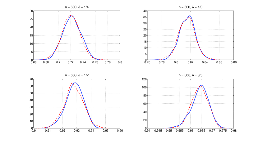
Figure 1. The probability density function of the distribution of $\max_{S\subset[n]:|S|=\lfloor\delta n\rfloor}\|v\|_{S}^{2}$ when $n=600$, based on $500$ samples. The blue curve is for $v$, a unit eigenvector of a matrix drawn from the GOE, while the red dashed curve corresponds to a unit eigenvector of a random symmetric Bernoulli matrix.

Our next result shows that these extreme order statistics concentrate around their expectation, even for relatively small values of $n$.

Theorem 2.10 (Concentration of the extreme order statistic).

Let $v$ be a random vector uniformly distributed on the unit sphere $S^{n-1}$. Then, for any $1\leq m\leq n$ and every $t\geq 0$,

(8) $$\mathbb{P}\Big{(}\Big{|}\max_{S\subset[n]:|S|=m}\|v\|_{S}-\mathbb{E}\max_{S\subset[n]:|S|=m}\|v\|_{S}\Big{|}>t\Big{)}\leq C\exp(-cnt^{2})$$

and

(9) $$\mathbb{P}\Big{(}\Big{|}\min_{S\subset[n]:|S|=m}\|v\|_{S}-\mathbb{E}\min_{S\subset[n]:|S|=m}\|v\|_{S}\Big{|}>t\Big{)}\leq C\exp(-cnt^{2})$$

where $C,c>0$ are absolute constants.

We prove these results in Section 10.

3. Direct comparison theorems

In many cases, one can compare the eigenvectors of a Wigner matrix directly to those of the GOE. In the random matrix theory literature, such results are often referred to as universality results.

Let $W$ be a Wigner matrix with atom variables $\xi,\zeta$. We will require that $\xi$ and $\zeta$ satisfy a few moment conditions. In particular, we say $\xi,\zeta$ are from the class $\mathcal{M}_{4}$ if

• $\xi$ and $\zeta$ are sub-exponential random variables,

• $\mathbb{E}(\xi)=\mathbb{E}(\zeta)=\mathbb{E}(\xi^{3})=0$, and

• $\mathbb{E}(\xi^{2})=1,\mathbb{E}(\xi^{4})=3,\mathbb{E}(\zeta^{2})=2$.

These conditions imply that the first four moments of the off-diagonal entries of $W$ match those of the GOE, and the first 2 moments of the diagonal entries of $W$ match those of the GOE.

Let $\{X_{n}\}_{n\geq 1}$ and $\{Y_{n}\}_{n\geq 1}$ be two sequences of real random variables. In order to show that they have (asymptotically) the same distribution, it suffices to show that

$$\mathbb{P}(X_{n}\leq t)-\mathbb{P}(Y_{n}\leq t)=o(1)$$

for all $t$. Notice that

$$\mathbb{P}(X_{n}\leq t)=\mathbb{E}f_{t}(X_{n}),$$

where $f_{t}(X_{n})$ is the indicator function of the event $\{X_{n}\leq t\}$. In practice, it is useful to smoothen $f_{t}$ a little bit to obtain a function with bounded derivatives, at the cost of an extra error term. We are going to use this strategy in the next few theorems, which allow us to compare $X_{n}$ with $Y_{n}$ by bounding $\mathbb{E}F(X_{n})-\mathbb{E}F(Y_{n})$ for a large set of test functions $F$.

One of the first universality results for eigenvectors is the following result.

Theorem 3.1 (Eigenvector coefficients of Wigner matrices, [78]).

Given $C>0$ and random variables $\xi,\zeta$ from the class $\mathcal{M}_{4}$, there are constants $\delta,C_{0}>0$ such that the following statement holds. Let $W$ be an $n\times n$ Wigner matrix with atom variables $\xi,\zeta$ and with unit eigenvectors $v_{1},\ldots,v_{n}$. Let $v_{i}(j)$ denote the $j$th entry of $v_{i}$. For $1\leq i,j\leq n$, let $Z_{i,j}$ be independent random variables with $Z_{i,j}\sim N(0,1)$ for $j>1$ and $Z_{i,1}\sim|N(0,1)|$. Let $1\leq k\leq n^{\delta}$, and let $1\leq i_{1}<\ldots<i_{k}\leq n$ and $1\leq j_{1}<\ldots<j_{k}\leq n$ be indices. Then

(10) $$\left|\mathbb{E}F\left((\sqrt{n}v_{i_{a}}(j_{b}))_{1\leq a,b\leq k}\right)-\mathbb{E}F\left((Z_{i_{a},j_{b}})_{1\leq a,b\leq k}\right)\right|\leq C_{0}n^{-\delta}$$

whenever $F:\mathbb{R}^{k^{2}}\to\mathbb{R}$ is a smooth function obeying the bounds

$$|F(x)|\leq C$$

and

$$|\nabla^{j}F(x)|\leq Cn^{\delta}$$

for all $x\in\mathbb{R}^{k^{2}}$ and $0\leq j\leq 5$.

Theorem 3.1 is essentially the first part of [78, Theorem 7]. The original theorem has $o(1)$ on the right-hand side of (10), but one can obtain the better bound $C_{0}n^{-\delta}$ using the same proof. The essence of this theorem is that any set of at most $n^{\delta}$ coordinates (which may come from different eigenvectors) behaves like a set of iid Gaussian random variables. Because of our normalization, requiring the first non-zero coordinate of the eigenvectors of $W$ to be positive, we cannot expect this coordinate to be close to a normal random variable. However, Theorem 3.1 shows that it is close in distribution to the absolute value of a standard normal random variable. Similar results were also obtained in [44] for the case when $k=O(1)$.

Another way to show that an eigenvector $v$ behaves like a random vector $u$ uniformly distributed on the unit sphere is to fix a unit vector $a$, and compare the distribution of the inner product $v\cdot a$ with $u\cdot a$. It is easy to show that $u\cdot a$ satisfies the central limit theorem. Namely, if $u_{n}$ is a random vector uniformly distributed on the unit sphere $S^{n-1}$ and $\{a_{n}\}$ is a sequence of unit vectors with $a_{n}\in S^{n-1}$, then

$$\sqrt{n}u_{n}\cdot a_{n}\longrightarrow N(0,1)$$

in distribution as $n\to\infty$. We refer the reader to [40] and [78, Proposition 25] for details and a proof of this statement. The following is a consequence of [78, Theorem 13].

Theorem 3.2 (Theorem 13 from [78]).

Let $\xi,\zeta$ be random variables from the class $\mathcal{M}_{4}$, and assume $\xi$ is a symmetric random variable. For each $n\geq 1$, let $W_{n}$ be an $n\times n$ Wigner matrix with atom variables $\xi,\zeta$. Let $\{a_{n}\}$ be a sequence of unit vectors with $a_{n}\in S^{n-1}$ such that $\lim_{n\to\infty}\|a_{n}\|_{\ell^{\infty}}=0$, and let $\{i_{n}\}$ be a sequence of indices with $i_{n}\in[n]$. Then

$$\sqrt{n}v_{i_{n}}(W_{n})\cdot a_{n}\longrightarrow N(0,1)$$

in distribution as $n\to\infty$.

In a recent paper [14], it was showed that one can remove the assumption that $\xi,\zeta$ are from the class $\mathcal{M}_{4}$, with an extra restriction on the index $i_{n}$.

Theorem 3.3 (Theorem 1.2 from [14]).

Let $\xi,\zeta$ be sub-exponetial random variables with mean zero, and assume $\xi$ has unit variance. For each $n\geq 1$, let $W_{n}$ be an $n\times n$ Wigner matrix with atom variables $\xi,\zeta$. In addition, let $\{a_{n}\}$ be a sequence of unit vectors with $a_{n}\in S^{n-1}$. Then there exists $\tilde{\delta}>0$ such that, for any fixed integer $m\geq 1$ and any

$$I_{n}\subset T_{n}:=\left([1,n^{1/4}]\cup[n^{1-\tilde{\delta}},n-n^{1-\tilde{\delta}}]\cup[n-n^{1/4},n]\right)\cap\mathbb{N}$$

with $|I_{n}|=m$,

$$\sqrt{n}(|a_{n}\cdot v_{i}(W_{n})|)_{i\in I_{n}}\longrightarrow(|Z_{i}|)_{i=1}^{m}$$

in distribution as $n\to\infty$, where $Z_{1},\ldots,Z_{m}$ are iid standard normal random variables.

One immediately obtains the following corollary

Corollary 3.4 (Corollary 1.3 from [14]).

Let $W_{n}$, $\tilde{\delta}$, and $T_{n}$ be as in Theorem 3.3. For each $n\geq 1$, let $i_{n}\in T_{n}$, and let $v_{i_{n}}^{(n)}(j)$ be the $j$th coordinate of $v_{i_{n}}(W_{n})$. Assume $l$ is a fixed positive integer. Then, for any $J_{n}\subset[n]$ with $|J_{n}|=l$,

$$\sqrt{n}\left(\left|v_{i_{n}}^{(n)}(j)\right|\right)_{j\in J_{n}}\longrightarrow(|Z_{j}|)_{j=1}^{l}$$

in distribution as $n\to\infty$, where $Z_{1},\ldots,Z_{l}$ are iid standard normal random variables.

Remark 3.5.

Both Theorem 3.3 and Corollary 3.4 hold for more general ensembles of random matrices than Wigner matrices. Indeed, the results in [14] hold for so-called generalized Wigner matrices, where the entries above the diagonal are only required to be independent, not necessarily identically distributed; see [14, Definition 1.1] for details.

4. Extremal coordinates

In this section, we investigate the largest and smallest coordinates (in absolute value) of an eigenvector of a Wigner matrix.

4.1. The largest coordinate

In view of Theorem 2.1, it is natural to conjecture that, for any eigenvector $v_{j}$,

(11) $$\|v_{j}\|_{\ell^{\infty}}=O\left(\sqrt{\frac{\log n}{n}}\right)$$

with high probability. The first breakthrough was made in [30, Theorem 5.1], which provides a bound of the form $\frac{\log^{O(1)}n}{\sqrt{n}}$ for a large proportion of eigenvectors $v_{j}$, under some technical conditions on the distribution of the entries. This result was extended to all eigenvectors under a weaker assumption in [74, 75], and many newer papers [22, 26, 29, 30, 31, 32, 33, 34, 35, 36, 37, 79, 85] give further strengthening and generalizations. In particular, the optimal bound in (11) was recently obtained in [85].

Theorem 4.1 (Optimal upper bound; Theorem 6.1 from [85]).

Let $\xi$ be a sub-gaussian random variable with mean zero and unit variance. Then, for any $C_{1}>0$ and any $0<\varepsilon<1$, there exists a constant $C_{2}>0$ such that the following holds. Let $W$ be an $n\times n$ Wigner matrix with atom variable $\xi$.

• (Bulk case) For any $\varepsilon n\leq i\leq(1-\varepsilon)n$,

  $$\|v_{i}(W)\|_{\ell^{\infty}}\leq C_{2}\sqrt{\frac{\log n}{n}}$$

  with probability at least $1-n^{-C_{1}}$.

• (Edge case) For $1\leq i\leq\varepsilon n$ or $(1-\varepsilon)n\leq i\leq n$,

  $$\|v_{i}(W)\|_{\ell^{\infty}}\leq C_{2}\frac{\log n}{\sqrt{n}}$$

  with probability at least $1-n^{-C_{1}}$.

Remark 4.2.

Theorem 4.1 was proved in [85] under the stronger assumption that $\xi$ is $K$-bounded for some constant $K$. One can easily obtain the more general result here by observing that [85, Lemma 1.2] holds under the sub-gaussian assumption, as a special case of a recent result, [64, Theorem 2.1]. The rest of the proof remains unchanged.

Using Theorem 3.1, one can derive a matching lower bound.

Theorem 4.3 (Matching lower bound).

Let $\xi,\zeta$ be random variables from the class $\mathcal{M}_{4}$. Then there exists a constant $c>0$ such that the following holds. Let $W$ be an $n\times n$ Wigner matrix with atom variables $\xi,\zeta$. For any $1\leq i\leq n$,

$$\|v_{i}(W)\|_{\ell^{\infty}}\geq c\sqrt{\frac{\log n}{n}}$$

with probability $1-o(1)$.

Open question. Prove the optimal bound in (11) for all eigenvectors (including the edge case). Open question. Is the limiting distribution of $\|v_{i}\|_{\ell^{\infty}}$ universal, or does it depend on the atom variables $\xi$ and $\zeta$?

One can deduce a slightly-weaker version of Theorem 4.1 when the entries are only assumed to be sub-exponential with exponent $0<\alpha<2$ by applying [85, Theorem 6.1] and a truncation argument. We apply such an argument in Section 12 to obtain the following corollary.

Corollary 4.4.

Let $\xi$ be a symmetric sub-exponential random variable with exponent $\alpha>0$. Assume further that $\xi$ has unit variance. Then, for any $C_{1}$ and $0<\varepsilon<1$, there is a constant $C_{2}$ such that the following holds. Let $W$ be an $n\times n$ Wigner matrix with atom variable $\xi$.

• (Bulk case) For any $\varepsilon n\leq i\leq(1-\varepsilon)n$,

  $$\|v_{i}(W)\|_{\ell^{\infty}}\leq C_{2}\sqrt{\frac{\log^{1+2/\alpha}n}{n}}$$

  with probability at least $1-n^{-C_{1}}$.

• (Edge case) For $1\leq i\leq\varepsilon n$ or $(1-\varepsilon)n\leq i\leq n$,

  $$\|v_{i}(W)\|_{\ell^{\infty}}\leq C_{2}\frac{\log^{1+2/\alpha}n}{\sqrt{n}}$$

  with probability at least $1-n^{-C_{1}}$.

Corollary 4.4 falls short of the optimal bound in (11); it remains an open question to obtain the optimal bound when the entries are not sub-gaussian.

Next, we discuss a generalization. Notice that $\|v\|_{\ell^{\infty}}=\max_{1\leq i\leq n}|v\cdot e_{i}|$, where $e_{1},\ldots,e_{n}$ are the standard basis vectors. What happens if we consider the inner product $v\cdot u$, for any fixed unit vector $u$? The theorems in the previous section show that, under certain technical assumptions, $\sqrt{n}v\cdot u$ is approximately Gaussian, which implies that $|v\cdot u|$ is typically of order $n^{-1/2}$. The following result gives a strong deviation bound.

Theorem 4.5 (Isotropic delocalization, Theorem 2.16 from [11]).

Let $\xi$ and $\zeta$ be zero-mean sub-exponential random variables, and assume that $\xi$ has unit variance. Let $W$ be an $n\times n$ Wigner matrix with atom variables $\xi,\zeta$. Then, for any $C_{1}>0$ and $0<\varepsilon<1/2$, there exists $C_{2}>0$ (depending only on $C_{1},\varepsilon$, $\xi$, and $\zeta$) such that

$$\sup_{1\leq i\leq n}|v_{i}\cdot u|\leq\frac{n^{\varepsilon}}{\sqrt{n}},$$

for any fixed unit vector $u\in S^{n-1}$, with probability at least $1-C_{2}n^{-C_{1}}$.

Remark 4.6.

Theorem 4.5 and the results in [11] actually hold for a larger class of so-called generalized Wigner matrices whose entries have bounded moments; see [11, Section 2.2] for details.

4.2. The smallest coordinate

We now turn our attention to the smallest coordinate of a given eigenvector. To this end, we recall the definition of $\|\cdot\|_{\min}$ given in (3).

Theorem 4.7 (Individual coordinates: Lower bound).

Let $\xi,\zeta$ be sub-gaussian random variables with mean zero, and assume $\xi$ has unit variance. Let $W$ be an $n\times n$ Wigner matrix with atom variables $\xi,\zeta$. Let $v_{1},\ldots,v_{n}$ denote the unit eigenvectors of $W$, and let $v_{i}(j)$ denote the $j$th coordinate of $v_{i}$. Then there exist constants $C,c,c_{0},c_{1}>0$ (depending only on $\xi,\zeta$) such that, for any $n^{-c_{0}}<\alpha<c_{0}$ and $\delta\geq n^{-c_{0}/\alpha}$,

$$\sup_{1\leq i,j\leq n}\mathbb{P}\left(|v_{i}(j)|\leq\frac{\delta}{\sqrt{n}(\log n)^{c_{1}}}\right)\leq C\frac{\delta}{\sqrt{\alpha}}+C\exp(-c\log^{2}n).$$

By the union bound, we immediately obtain the following corollary.

Corollary 4.8.

Let $\xi,\zeta$ be sub-gaussian random variables with mean zero, and assume $\xi$ has unit variance. Let $W$ be an $n\times n$ Wigner matrix with atom variables $\xi,\zeta$. Let $v_{1},\ldots,v_{n}$ denote the unit eigenvectors of $W$, and let $v_{i}(j)$ denote the $j$th coordinate of $v_{i}$. Then there exist constants $C,c,c_{0},c_{1}>0$ (depending only on $\xi,\zeta$) such that, for any $n^{-c_{0}}<\alpha<c_{0}$ and $\delta\geq n^{-c_{0}/\alpha}$,

$$\sup_{1\leq i\leq n}\mathbb{P}\left(\|v_{i}(W)\|_{\min}\leq\frac{\delta}{n^{3/2}(\log n)^{c_{1}}}\right)\leq C\frac{\delta}{\sqrt{\alpha}}+C\exp(-c\log^{2}n).$$

In particular, Corollary 4.8 implies that, with high probability,

$$\|v_{i}(W)\|_{\min}=\Omega\left(\frac{1}{n^{3/2}(\log n)^{c_{1}}}\right).$$

In view of Theorem 2.1, this is optimal up to logarithmic factors.

Open question. Is the limiting distribution of $\|v_{j}(W)\|_{\min}$ universal, or does it depend on the atom variables $\xi$ and $\zeta$?

We prove Corollary 4.4 and Theorem 4.7 in Section 12.

5. No-gaps delocalization

The results in the previous section address how much mass can be contained in a single coordinate. We next turn to similar estimates for the amount of mass contained on a number of coordinates. In particular, the following results assert that any subset of coordinates of linear size must contain a non-negligible fraction of the vector’s $\ell^{2}$-norm. Following Rudelson and Vershynin [65], we refer to this phenomenon as no-gaps delocalization.

Using Corollary 3.4, we obtain the following analogue of Theorem 2.7. Recall the function $H$ defined in (7).

Theorem 5.1.

Let $W_{n}$, $\tilde{\delta}$, and $T_{n}$ be as in Theorem 3.3. For each $n$, let $k_{n}\in T_{n}$. Let $v_{k_{n}}$ be a unit eigenvector of $W_{n}$ corresponding to $\lambda_{k_{n}}(Y_{n})$. Then, for any fixed $0<\delta<1$,

$$\max_{S\subset[n]:|S|=\lfloor\delta n\rfloor}\|v_{k_{n}}\|_{S}^{2}\longrightarrow-\int_{0}^{\delta}H(u)\,du$$

and

$$\min_{S\subset[n]:|S|=\lfloor\delta n\rfloor}\|v_{k_{n}}\|_{S}^{2}\longrightarrow-\int_{1-\delta}^{1}H(u)\,du$$

in probability as $n\to\infty$, where $H$ is defined in (7).

We prove Theorem 5.1 in Section 13. The integrals in the right-hand side involving $H$ can be expressed in a number of different ways; see Remarks 2.8 and 2.9 for details. In particular, Remark 2.9 shows that, for $\delta$ sufficiently small, the first integral is $\Theta(\delta\log(\delta^{-1}))$ and the second is $\Theta(\delta^{3})$.

While this survey was written, Rudelson and Vershynin posted the following theorem, which addresses the lower bound for more general models of random matrices. Their proof is more involved and very different from that of Theorem 5.1.

Theorem 5.2 (Theorem 1.5 from [65]).

Let $\xi$ be a real random variable which satisfies

$$\sup_{u\in\mathbb{R}}\mathbb{P}(|\xi-u|\leq 1)\leq 1-p\quad\text{and}\quad\mathbb{P}(|\xi|>K)\leq p/2$$

for some $K,p>0$. Let $W$ be an $n\times n$ Wigner matrix with atom variable $\xi$. Let $\kappa\geq 1$ be such that the event $\mathcal{B}_{\kappa}:=\{\|W\|\leq\kappa\sqrt{n}\}$ holds with probability at least $1/2$. Let $\delta\geq 1/n$ and $t\geq c_{1}\delta^{-7/6}n^{-1/6}+e^{-c_{2}/\sqrt{\delta}}$. Then, conditionally on $\mathcal{B}_{\kappa}$, the following holds with probability at least $1-(c_{3}t)^{\delta n}$: every eigenvector $v$ of $W$ satisfies

$$\min_{S\subset[n]:|S|\geq\delta n}\|v\|_{S}\geq(\delta t)^{6}.$$

Here, the constants $c_{1},c_{2},c_{3}>0$ depend on $p$, $K$, and $\kappa$.

Remark 5.3.

The results in [65] hold for even more general ensembles of random matrices than what is stated above; see [65, Assumption 1.1] for details. For many atom variables $\xi,\zeta$, the spectral norm $\|W\|$ is strongly concentrated (see Lemma 11.3 or [73, Corollary 2.3.6] for examples), so the event $\mathcal{B}_{\kappa}$ holds with high probability, provided $\kappa$ is sufficiently large.

Compared to Theorem 5.1, the estimate in Theorem 5.2 is not optimal. On the other hand, the probability bound in Theorem 5.2 is stronger and thus the estimate is more applicable. It would be desirable to have a common strengthening of these two theorems. This can be done by achieving an extension of Theorem 2.10.

Open question. Extend Theorem 2.10 to eigenvectors of Wigner matrices with non-gaussian entries.

We conclude this section with the following corollary, which is comparable to Theorem 2.2.

Corollary 5.4 ($\ell^{p}$-norm).

Let $\xi$, $\zeta$ be real sub-gaussian random variables with mean zero, and assume $\xi$ has unit variance. Let $W$ be an $n\times n$ Wigner matrix with atom variables $\xi$, $\zeta$. Then, for any $1\leq p\leq 2$, there exist constants $C,c,C_{0},c_{0}>0$ (depending only on $p$ and the sub-gaussian moments of $\xi$ and $\zeta$) such that

$$c_{0}n^{1/p-1/2}\leq\min_{1\leq j\leq n}\|v_{j}(W)\|_{\ell^{p}}\leq\max_{1\leq j\leq n}\|v_{j}(W)\|_{\ell^{p}}\leq C_{0}n^{1/p-1/2}$$

with probability at least $1-C\exp(-cn)$.

One-sided bounds for $\|v_{j}(W)\|_{\ell^{p}}$ were previously obtained in [30]. We give a proof of Corollary 5.4 in Section 13.

6. Random symmetric matrices with non-zero mean

In this section, we consider random symmetric matrices with nonzero mean, which includes the adjacency matrices $A_{n}(p)$ and $\tilde{A}_{n}(p)$. In view of Definition 1.1, we do not refer to these matrices as Wigner matrices. However, such random symmetric matrices can be written as deterministic perturbations of Wigner matrices, and we will often take advantage of this fact.

It has been observed that the unit eigenvector corresponding to the largest eigenvalue of the adjacency matrix $A_{n}(p)$ looks like the normalized all-ones vector $\frac{1}{\sqrt{n}}\mathbf{1}_{n}$, since the degree of the vertices are approximately the same (assuming $p\gg\log n/n$). For the rest of the spectrum, we expect the corresponding eigenvectors to be uniformly distributed on the unit sphere in $\mathbb{R}^{n}$.

6.1. The largest eigenvector

The following result describes the unit eigenvector corresponding to the largest eigenvalue of $A_{n}(p)$

Theorem 6.1 (Theorem 1 from [50]).

Let $A_{n}(p)$ be the adjacency matrix of the random graph $G(n,p)$. Let $v_{n}$ be a unit eigenvector corresponding to the largest eigenvalue of $A_{n}(p)$. For $p\geq\frac{\log^{6}n}{n}$,

$$\left\|v_{n}-\frac{1}{\sqrt{n}}\mathbf{1}_{n}\right\|_{\ell^{\infty}}\leq C\frac{\log n}{\log(np)}\frac{1}{\sqrt{n}}\sqrt{\frac{\log n}{np}}$$

with probability $1-o(1)$, for some constant $C>0$.

6.2. Extremal coordinates

Recall that $\tilde{G}(n,p)$ is the Erdös–Rényi random graph with loops on $n$ vertices and edge density $p$. We have the following analogue of Theorem 4.1.

Theorem 6.2 (Theorem 2.16 from [26]).

Let $\tilde{A}_{n}(p)$ be the adjacency matrix of the random graph $\tilde{G}(n,p)$, and let $\tilde{v}_{i}$ be the unit eigenvector corresponding to the $i$th smallest eigenvalue. Fix $1+\varepsilon_{0}\leq\alpha\leq C_{0}\log\log n$ for some constants $\varepsilon_{0},C_{0}>0$. Assume $c^{\prime}\geq p\geq(\log n)^{6\alpha}/n$ for some constant $c^{\prime}$. Then there exist constants $C,c>0$ (depending on $\varepsilon_{0}$, $C_{0}$, and $c^{\prime}$) such that

$$\max_{1\leq i\leq n-1}\|\tilde{v}_{i}\|_{\ell^{\infty}}\leq\frac{(\log n)^{4\alpha}}{\sqrt{n}}$$

and

$$\left\|\tilde{v}_{n}-\frac{1}{\sqrt{n}}\mathbf{1}_{n}\right\|_{\ell^{\infty}}\leq C\frac{(\log n)^{\alpha}}{\sqrt{n}}\sqrt{\frac{1}{np}}$$

with probability at least $1-C\exp(-c(\log n)^{\alpha})$.

An upper bound for the $\ell^{\infty}$-norm of the form $\frac{\log^{C}n}{\sqrt{n}}$ was originally proven in [81] for fixed values of $p$. Theorem 6.2 above is an extension which applies to a wider range of values of $p$. More generally, the results in [26] also apply to perturbed Wigner matrices.

Theorem 6.3 (Theorem 2.16 from [26]).

Let $\xi$ be a sub-exponential random variable with mean zero and unit variance. Let $W$ be the $n\times n$ Wigner matrix with atom variable $\xi$. Fix $\mu\in\mathbb{R}$, and consider the matrix $M:=W+\mu\mathbf{J}$, where $\mathbf{J}$ is the all-ones matrix. Fix $1+\varepsilon_{0}\leq\alpha\leq C_{0}\log\log n$ for some constants $\varepsilon_{0},C_{0}>0$. Then there exists $C,c>0$ (depending on $\varepsilon_{0},C_{0}$, $\xi$, and $\mu$) such that

$$\max_{1\leq i\leq n-1}\|v_{i}(M)\|_{\ell^{\infty}}\leq\frac{(\log n)^{4\alpha}}{\sqrt{n}}$$

and

$$\left\|v_{n}(M)-\frac{1}{\sqrt{n}}\mathbf{1}_{n}\right\|_{\ell^{\infty}}\leq C\frac{(\log n)^{\alpha}}{n}$$

with probability at least $1-C\exp(-c(\log n)^{\alpha})$.

We next consider the smallest coordinates of each eigenvector of the adjacency matrix $A_{n}(p)$. We prove the following analogue of Theorem 4.7

Theorem 6.4 (Individual coordinates: Lower bound).

Let $A_{n}(p)$ be the adjacency matrix of the random graph $G(n,p)$ for some fixed value of $p\in(0,1)$. Let $v_{1},\ldots,v_{n}$ be the unit eigenvectors of $A_{n}(p)$, and let $v_{i}(j)$ denote the $j$th coordinate of $v_{i}$. Then, for any $\alpha>0$, there exist constants $C,c_{1}>0$ (depending on $p,\alpha$) such that, for any $\delta>n^{-\alpha}$,

$$\sup_{1\leq i\leq n-1}\sup_{1\leq j\leq n}\mathbb{P}\left(|v_{i}(j)|\leq\frac{\delta}{\sqrt{n}(\log n)^{c_{1}}}\right)\leq Cn^{o(1)}\delta+o(1).$$

Here, the rate of convergence to zero implicit in the $o(1)$ terms depends on $p,\alpha$.

Notice that Theorem 6.4 does not address the eigenvector corresponding to the largest eigenvalue of $A_{n}(p$). Bounds for this eigenvector can easily be obtained using Theorem 6.1 and are left as an exercise.

6.3. No-gaps delocalization

In [20], the following result is developed as a tool in the authors’ study of nodal domain for the eigenvectors of $G(n,p)$.

Theorem 6.5 (Theorem 3.1 from [20]).

Let $A_{n}(p)$ be the adjacency matrix of the random graph $G(n,p)$, and let $v_{i}$ be the unit eigenvector corresponding to the $i$th smallest eigenvalue. For every $p\in(0,1)$ and every $\varepsilon>0$, there exist $C,c,\eta>0$ (depending on $\varepsilon$ and $p$) such that, for every fixed subset $S\subset[n]$ of size $|S|\geq(\frac{1}{2}+\varepsilon)n$,

$$\min_{1\leq i\leq n-1}\|v_{i}\|_{S}\geq\eta$$

with probability at least $1-C\exp(-cn)$.

Theorem 6.5 is not nearly as strong as Theorem 5.2 in Section 5, which holds for all subsets $S\subset[n]$ of specified size. However, the results from [65] do not apply directly to the adjacency matrix $A_{n}(p)$. In particular, Theorem 5.2 only applies when the spectral norm of the matrix is $O(\sqrt{n})$ with high probability. However, the largest eigenvalue of $A_{n}(p)$ is of order $\Theta(n)$.

We conclude this section by discussing some variations which do not require the spectral norm to be $O(\sqrt{n})$. Specifically, we consider eigenvectors of matrices of the form $M:=W+J$, where $W$ is a Wigner matrix and $J$ is a real symmetric deterministic low-rank matrix. When $W$ is drawn from the GOE, it suffices to consider the case that $J$ is diagonal (since $W$ is invariant under conjugation by orthogonal matrices). Thus, we begin with the case when $J$ is diagonal.

Theorem 6.6 (Diagonal low-rank perturbations).

Let $\xi$, $\zeta$ be real sub-gaussian random variables with mean zero, and assume $\xi$ has unit variance. Let $W$ be an $n\times n$ Wigner matrix with atom variables $\xi$, $\zeta$; let $J$ be $n\times n$ deterministic, diagonal real symmetric matrix with rank $k$. Let $M:=W+J$, and consider $\lambda_{j}(M)\in[\lambda_{1}(W),\lambda_{n}(W)]$ and its corresponding unit eigenvector $v_{j}(M)$. For any constant $\delta\in(0,1)$ and any fixed set $S\subset[n]$ with size $|S|=\lfloor\delta n\rfloor$, there exist constants $C,c>0$ and $0<\eta_{1}\leq\eta_{2}<1$ (depending only on $\delta$, $k$, and the sub-gaussian moments of $\xi$ and $\zeta$) such that

$$\eta_{2}\geq\|v_{j}(M)\|_{S}\geq\eta_{1}$$

with probability at least $1-C\exp\left(-c(\log n)^{c\log\log n}\right)$.

Theorem 6.6 does not handle the eigenvectors corresponding to the extreme eigenvalues of $M$ due to the condition $\lambda_{j}(M)\in[\lambda_{1}(W),\lambda_{n}(W)]$. In particular, it is possible for the eigenvectors corresponding to the largest and smallest eigenvalues to be localized for certain choices of the diagonal matrix $J$. A localized eigenvector is an eigenvector whose mass in concentrated on only a few coordinates. We present an example of this phenomenon in the following theorem.

Theorem 6.7.

Let $\xi$, $\zeta$ be real sub-gaussian random variables with mean zero and unit variance. Then there exist constants $C,c>0$ such that the following holds. Let $W$ be an $n\times n$ Wigner matrix with atom variables $\xi$, $\zeta$. Let $J=\sqrt{n}\theta e_{k}e_{k}^{\mathrm{T}}$ for some $\theta>C$ and $1\leq k\leq n$, where $e_{1},\ldots,e_{n}$ is the standard basis of $\mathbb{R}^{n}$. Set $M:=W+J$. Then

$$|v_{n}(M)\cdot e_{k}|^{2}\geq 1-\frac{C^{2}}{\theta^{2}}$$

with probability at least $1-C\exp(-cn)$.

Specifically, Theorem 6.7 implies that for $\theta$ large enough (say, $\theta=\Omega(\log n)$), most of the mass of the eigenvector $v_{n}(M)$ is concentrated on the $k$th coordinate. This is in contrast to Theorem 6.6, which shows that, with high probability, the other eigenvectors cannot concentrate on a single coordinate. Theorem 6.7 is part of a large collection of results concerning the extreme eigenvalues and eigenvectors of perturbed random matrices. We refer the reader to [5, 9, 45, 55, 58, 60] and references therein for many other results.

Theorem 6.7 follows as a simple corollary of a slightly-modified version of the Davis–Kahan $\sin\theta$ Theorem (see, for instance, [55, Theorem 4]) and a bound on the spectral norm of a Wigner matrix (Lemma 11.3); we leave the details as an exercise.

Theorems 6.6 and 6.7 both deal with diagonal perturbations. For more general perturbations, we have the following result.

Theorem 6.8 (General low-rank perturbations).

Let $\xi$, $\zeta$ be real sub-gaussian random variables with mean zero, and assume $\xi$ has unit variance. Let $W$ be an $n\times n$ Wigner matrix with atom variables $\xi$, $\zeta$; let $J$ be $n\times n$ deterministic real symmetric matrix with rank $k$. Let $\varepsilon_{1},\varepsilon_{0}>0$. Let $M:=W+J$, and consider $\lambda_{j}(M)$ such that $\varepsilon_{1}n\leq j\leq(1-\varepsilon_{1})n$ and its corresponding unit eigenvector $v_{j}(M)$. For any constant $\delta\in(0,1)$ and any fixed set $S\subset[n]$ with size $|S|=\lfloor\delta n\rfloor$, there exist constants $C,c>0$ and $0<\eta<1$ (depending only on $\delta$, $k$, $\varepsilon_{0}$, $\varepsilon_{1}$, and the sub-gaussian moments of $\xi$ and $\zeta$) such that

$$\mathbb{P}\left(\frac{1}{n^{1-\varepsilon_{0}}}\leq\|v_{j}(M)\|_{S}\leq\eta\right)\leq C\exp\left(-c(\log n)^{c\log\log n}\right).$$

Remark 6.9.

Theorem 6.8 shows that, with high probability, either $\|v_{j}(M)\|_{S}\geq\eta$ or $\|v_{j}(M)\|_{S}\leq\frac{1}{n^{1-\varepsilon_{0}}}$. Based on the previous results, we do not expect the later case to be a likely event. However, it appears additional structural information about $J$ (for instance, that $J$ is diagonal as in Theorem 6.6) is required to eliminate this possibility. See the proof of Theorem 6.8 for additional details.

In the case when $J$ has rank one, we have the following.

Theorem 6.10 (Rank one perturbations).

Let $\xi$, $\zeta$ be real sub-gaussian random variables with mean zero and unit variance, and fix $\varepsilon_{1}>0$. Then there exist constants $C,c>0$ such that the following holds. Let $W$ be an $n\times n$ Wigner matrix with atom variables $\xi$, $\zeta$. Suppose $J=\theta uu^{\mathrm{T}}$, where $\theta\in\mathbb{R}$ and $u\in\mathbb{R}^{n}$ is a unit vector. Set $M:=W+J$. Then, for any integer $j$ with $\varepsilon_{1}n\leq j\leq(1-\varepsilon_{1})n$,

$$|v_{j}(M)\cdot u|\leq\frac{C(\log n)^{c\log\log n}}{|\theta|}$$

with probability $1-o(1)$.

When $\theta:=\mu n$ and $u:=n^{-1/2}\mathbf{1}_{n}$, $J$ becomes the matrix in which every entry takes the value $\mu$. In this case, the entries of $W+J$ have mean $\mu$ instead of mean zero. Thus, applying Theorem 6.10, we immediately obtain the following corollary.

Corollary 6.11 (Wigner matrices with non-zero mean).

Let $\xi$, $\zeta$ be real sub-gaussian random variables with mean zero and unit variance, and fix $\varepsilon_{1}>0$. Then there exist constants $C,c>0$ such that the following holds. Let $\mu\in\mathbb{R}$ with $\mu\neq 0$. Let $W$ be an $n\times n$ Wigner matrix with atom variables $\xi$, $\zeta$. Set $M:=W+\mu\mathbf{J}$, where $\mathbf{J}$ is the all-ones matrix. Then, for any integer $j$ with $\varepsilon_{1}n\leq j\leq(1-\varepsilon_{1})n$,

$$|v_{j}(M)\cdot\mathbf{1}_{n}|\leq\frac{C(\log n)^{c\log\log n}}{|\mu|\sqrt{n}}$$

with probability $1-o(1)$.

We prove Theorems 6.4, 6.6, 6.8 and 6.10 in Section 14.

7. Localized eigenvectors: Heavy-tailed and band random matrices

As we saw in Theorem 6.7, the eigenvectors corresponding to the extreme eigenvalues of a perturbed Wigner matrix can be localized, meaning that most of the mass is contained on only a few coordinates. For instance, in Theorem 6.7, most of the mass was contained on a single coordinate. We now discuss a similar phenomenon for heavy-tailed and band random matrices.

7.1. Heavy-tailed random matrices

Most of the results from the previous sections required the atom variables $\xi$, $\zeta$ to be sub-exponential or sub-gaussian. In particular, these conditions imply that $\xi$ and $\zeta$ have finite moments of all orders. In other words, the atom variables have very light tails. We now consider the case when the atom variables have heavy tails, such as when $\xi$ and $\zeta$ have only one or even zero finite moments. In this case, the eigenvectors corresponding to the largest eigenvalues behave very differently than predicted by the results above.

Theorem 7.1 (Theorem 1.1 from [8]).

Let $\xi$ be a real random variable satisfying

$$\mathbb{P}(|\xi|\geq x)=L(x)x^{-\alpha}$$

for all $x>0$, where $0<\alpha<2$ and $L:(0,\infty)\to(0,\infty)$ is a slowly varying function, i.e., for all $t>0$,

$$\lim_{x\to\infty}\frac{L(tx)}{L(x)}=1.$$

For each $n\geq 1$, let $W_{n}$ be an $n\times n$ Wigner matrix with atom variable $\xi$. Fix an integer $k\geq 0$. Then, for every fixed $\varepsilon>0$,

$$\|v_{n-k}(W_{n})\|_{\ell^{\infty}}\geq\frac{1}{\sqrt{2}}-\varepsilon$$

with probability $1-o(1)$. In addition,

$$\min_{S\subset[n]:|S|=n-2}\|v_{n-k}(W_{n})\|_{S}\longrightarrow 0$$

in probability as $n\to\infty$.

Remark 7.2.

Theorem 7.1 also holds when $2\leq\alpha<4$ provided the atom variable $\xi$ is symmetric; see [8, Theorem 1.1] for details.

Theorem 7.1 shows that the eigenvectors corresponding to the largest eigenvalues of $W_{n}$ are concentrated on at most two coordinates. This is considerably different than the cases discussed above when $\xi$ has light tails.

Let us try to explain this phenomenon based on the tail behavior of $\xi$. It is well known that the largest entry of an $n\times n$ Wigner matrix with sub-gaussian entries is $O(\sqrt{\log n})$ with high probability. However, when the tails are heavy, the maximum entry of $W_{n}$ can be significantly larger. It was observed by Soshnikov [68, 69] that, in this case, the largest eigenvalues behave like the largest entries of the matrix. Intuitively, the eigenvector corresponding to the largest eigenvalue of $W_{n}$ should localize on the coordinates which match the largest entry. Since $W_{n}$ is symmetric, the largest entry can appear at most twice. Hence, we expect this eigenvector to be concentrated on at most two coordinates. This heuristic has led to a number of results regarding the eigenvalues and eigenvectors of heavy-tailed Wigner matrices; we refer the reader to [3, 7, 8, 12, 13, 17, 68, 69] and references therein for further details and additional results.

7.2. Random band matrices

The standard basis elements $e_{1},\ldots,e_{n}$ of $\mathbb{R}^{n}$ are always eigenvectors of an $n\times n$ diagonal matrix. In other words, the eigenvectors of a diagonal matrix are localized. Band matrices generalize diagonal matrices by only allowing the entries on and near the diagonal to be non-zero while requiring the other entries, away from the diagonal, to be zero.

We can form random band matrices from Wigner matrices. Indeed, let $W$ be an $n\times n$ Wigner matrix with atom variables $\xi$, $\zeta$. For simplicity, let us assume that $\xi$ and $\zeta$ are sub-gaussian random variables. We can form an $n\times n$ random band matrix $T$ from $W$ with band width $L\geq 1$ by replacing the $(i,j)$-entry of $W$ by zero if and only if $|i-j|\geq L$. Hence, the $(i,j)$-entry of $T$ is just the $(i,j)$-entry of $W$ when $|i-j|<L$. A random band matrix with width $n$ is a Wigner matrix, and a random band matrix with band width $1$ is a diagonal matrix. Thus, we expect a transition in the eigenvector behavior when the band width $L$ interpolates between $1$ and $n$. Indeed, it is conjectured that for $L$ significantly smaller than $\sqrt{n}$, the eigenvectors will be localized (with localization length on the order of $L^{2}$). On the other hand, for $L$ sufficiently larger than $\sqrt{n}$, it is expected that the eigenvectors of $T$ behave more like the eigenvectors of $W$. Some partial results in this direction have been established in [23, 24, 27, 66].

While random band matrices can be constructed from Wigner matrices, they are, in general, not Wigner matrices, and we will not focus on them here. We refer the interested reader to [8, 23, 24, 27, 66, 70] and references therein for results concerning the spectral properties of random band matrices. In the discussion above, we have focused on the case when the atom variables $\xi$ and $\zeta$ are sub-gaussian. However, Theorem 7.1 can be extended to random band matrices constructed from heavy-tailed Wigner matrices; see [8] for details.

8. Singular vectors and eigenvectors of non-Hermitian matrices

In this section, we consider the singular vectors and eigenvectors of non-Hermitian random matrices.

Let $M$ be a $p\times n$ matrix with real entries. Recall that the singular values of $M$ are the square roots of the eigenvalues of $MM^{\mathrm{T}}$. The left singular vectors are the eigenvectors of $MM^{\mathrm{T}}$, and the right singular vectors are the eigenvectors of $M^{\mathrm{T}}M$. Following our previously introduced notation, we will write

$$\sqrt{\lambda_{1}(MM^{\mathrm{T}})},\ldots,\sqrt{\lambda_{p}(MM^{\mathrm{T}})}$$

to denote the singular values and

$$v_{1}(MM^{\mathrm{T}}),\ldots,v_{p}(MM^{\mathrm{T}})$$

to denote the left singular vectors of $M$.

Let $M=M_{p,n}=(\zeta_{ij})_{1\leq i\leq p,1\leq j\leq n}$ be a random matrix (more specifically, a sequence of random matrices) whose entries are independent real random variables with mean zero and unit variance. Assume $\lim_{n\to\infty}p/n=y$ for some $y\in(0,1]$. The delocalization properties of the singular vectors of $M_{p,n}$ have been explored in [16, 57, 77, 85, 86]. The optimal bound of $O(\sqrt{\log n/n})$ for the $\ell^{\infty}$-norm was obtained recently in [85].

Theorem 8.1 (Delocalization of singular vectors, Theorem B.3 from [85]).

Let $\zeta$ be a sub-gaussian random variable with mean zero and unit variance. Then, for any $C_{1}>0$ and any $0<\varepsilon<1$, there exists a constant $C_{2}>0$ such that the following holds. Assume the entries of $M_{p,n}=(\zeta_{ij})_{1\leq i\leq p,1\leq j\leq n}$ are iid copies of $\zeta$. Let $a:=(1-\sqrt{y})^{2}$ and $b:=(1+\sqrt{y})^{2}$.

• (Bulk case) For any $1\leq i\leq n$ such that $\frac{1}{n}\lambda_{i}(M_{p,n}M_{p,n}^{\mathrm{T}})\in[a+\varepsilon,b-\varepsilon]$, there is a corresponding left singular vector $v_{i}(M_{p,n}M_{p,n}^{\mathrm{T}})$ such that

  $$\|v_{i}(M_{p,n}M_{p,n}^{\mathrm{T}})\|_{\ell^{\infty}}\leq C_{2}\sqrt{\frac{\log n}{{n}}}$$

  with probability at least $1-n^{-C_{1}}$. The same also holds for right singular vectors.

• (Edge case) For any $1\leq i\leq n$ such that $\frac{1}{n}\lambda_{i}(M_{p,n}M_{p,n}^{\mathrm{T}})\in[a-\varepsilon,a+\varepsilon]\cup[b-\varepsilon,b+\varepsilon]$ if $a\neq 0$ and $\frac{1}{n}\lambda_{i}(M_{p,n}M_{p,n}^{\mathrm{T}})\in[4-\varepsilon,4]$ if $a=0$, there is a corresponding left singular vector $v_{i}(M_{n,p}M_{n,p}^{\mathrm{T}})$ such that

  $$\|v_{i}(M_{n,p}M_{n,p}^{\mathrm{T}})\|_{\ell^{\infty}}\leq C_{2}\frac{\log n}{\sqrt{n}}$$

  with probability at least $1-n^{-C_{1}}$. The same also holds for right singular vectors.

Similar to Theorem 4.1 this was first proved under the stronger assumption that the entries of the matrix are bounded, but one can obtain this version using the same argument as in Remark 4.2. The analogue of Theorem 8.1 for the eigenvectors of $M_{n,n}$ was recently proved in [63], using a completely different method.

Theorem 8.2 (Delocalization of eigenvectors; Theorem 1.1 from [63]).

Let $M=(\zeta_{ij})_{1\leq i,j\leq n}$ be an $n\times n$ random matrix whose entries are independent real random variables with mean zero, variance at least one, and

$$\sup_{p\geq 1}p^{-1/2}(\mathbb{E}|\zeta_{ij}|^{p})^{1/p}\leq K$$

for all $1\leq i,j\leq n$. Then, for any $t\geq 2$, with probability at least $1-n^{1-t}$, all unit eigenvectors $v$ of $M$ satisfy

$$\|v\|_{\ell^{\infty}}\leq\frac{Ct^{3/2}\log^{9/2}n}{\sqrt{n}},$$

where $C$ depends only on $K$.

Remark 8.3.

The above result holds for more general matrix ensembles, e.g. random matrices with independent sub-exponential entries; see [63, Corollary 1.5] for details.

9. Random regular graphs

We now turn to the eigenvectors of the adjacency matrix of random regular graphs. Recall that a regular graph is a simple graph where each vertex has the same degree, and a $d$-regular graph is a regular graph with vertices of degree $d$. It is well-known that a $d$-regular graph on $n$ vertices exists if and only if $n\geq d+1$ and $nd$ is even. Let $G_{n,d}$ denote a random $d$-regular graph chosen uniformly from all $d$-regular graphs on $n$ vertices. It is easy to see that the adjacency matrix of $G_{n,d}$ has a trivial eigenvector $\frac{1}{\sqrt{n}}\mathbf{1}_{n}$ corresponding to the eigenvalue $d$. Further, it has been conjectured that every non-trivial unit eigenvector behaves like a uniform vector on the unit sphere.

In the combinatorics/computer science literature, the most interesting case to consider is when $d$ is a constant. This also seems to be the most difficult case to study. In this case, the strongest delocalization result known to the authors is the following, which is a corollary of [15, Theorem 1]

Theorem 9.1 (Theorem 1 from [15]).

Let $d$ be fixed and $\varepsilon>0$. Then there is a constant $\delta>0$ (depending on $d$ and $\varepsilon$) such that the following holds. With probability $1-o(1)$, for any unit eigenvector $v$ of the adjacency matrix of $G_{n,d}$, any subset $S\subset[n]$ satisfying

$$\|v\|_{S}^{2}>\varepsilon$$

must be of size $|S|\geq n^{\delta}.$

From [21], one has the following result for the eigenvectors in the case when $d$ grows slowly with the vertex size $n$.

Theorem 9.2 (Theorem 3 from [21]).

Fix $\delta>0$. Let $d:=d_{n}=(\log n)^{\gamma}$ for $\gamma>0$. Let $\eta_{n}:=(r_{n}-r_{n}^{-1})/2$ where $r_{n}:=\exp(d_{n}^{-\alpha})$ for some $0<\alpha<\min(1,\gamma^{-1})$. Let $T_{n}\subset[n]$ be a deterministic set of size $L_{n}=o(\eta_{n}^{-1})$. Let $\Omega_{n}$ be the event that some unit eigenvector $v$ of the adjacency matrix of $G_{n,d}$ satisfies $\|v\|_{T_{n}}^{2}\geq 1-\delta$. Then, for all sufficiently large $n$,

$$\mathbb{P}(\Omega_{n}^{c})\geq e^{-L_{n}\eta_{n}/d_{n}}\left(1-o(d_{n}^{-1})\right)=1-o(d_{n}^{-1}).$$

Finally, let us mention the following recent result from [6], which provides a near optimal bound when $d$ grows sufficiently fast with $n$.

Theorem 9.3 (Corollary 1.2 from [6]).

There exist constants $C,C^{\prime}>0$ such that the following holds. Let $C^{-1}\log^{4}n\leq d\leq Cn^{2/3}\log^{-4/3}n$. Then any unit eigenvector $v$ of the adjacency matrix of $G_{n,d}$ satisfies

$$\|v\|_{\ell^{\infty}}\leq C^{\prime}\frac{\log^{2}n}{\sqrt{n}}$$

with probability at least $1-\exp(-2\log^{2}n\cdot\log\log n)$.

Remark 9.4.

More generally, the results in [6] hold for other models of random regular graphs besides the uniform model $G_{n,d}$ discussed here; see [6, Section 1.2] for details.

10. Proofs for the Gaussian orthogonal ensemble

In order to prove the results in Section 2, we will need the following characterization of a unit vector uniformly distributed on the unit sphere $S^{n-1}$.

Lemma 10.1.

Let $v$ be a random vector uniformly distributed on the unit sphere $S^{n-1}$. Then $v$ has the same distribution as

$$\left(\frac{\xi_{1}}{\sqrt{\sum_{j=1}^{n}\xi_{j}^{2}}},\ldots,\frac{\xi_{n}}{\sqrt{\sum_{j=1}^{n}\xi_{j}^{2}}}\right)$$

where $\xi_{1},\ldots,\xi_{n}$ are iid standard normal random variables.

Proof.

The claim follows from the fact that the Gaussian vector $(\xi_{k})_{k=1}^{n}$ is rotationally invariant. We refer the reader to [43] for further details and other interesting results regarding entries of uniformly distributed unit vectors, and, more generally, results concerning entries of orthogonal matrices distributed according to Haar measure. ∎

We now prove Theorem 2.1. In order to do so, we will need the following result from [46].

Lemma 10.2 (Lemma 1 from [46]).

Suppose $X$ is a $\chi^{2}$-distributed with $k$ degrees of freedom. Then, for all $t>0$,

$$\mathbb{P}(X-k\geq 2\sqrt{kt}+2t)\leq\exp(-t)$$

and

$$\mathbb{P}(k-X\geq 2\sqrt{kt})\leq\exp(-t).$$

Proof of Theorem 2.1.

In view of Lemma 10.1, it suffices to assume that

$$v:=\left(\frac{\xi_{1}}{\sqrt{\sum_{j=1}^{n}\xi_{j}^{2}}},\ldots,\frac{\xi_{n}}{\sqrt{\sum_{j=1}^{n}\xi_{j}^{2}}}\right),$$

where $\xi_{1},\ldots,\xi_{n}$ are iid standard normal random variables.

We first verify (4). Let $C>1$ and $c_{1}=1/C<1$. Define the events

$$\Omega_{1}:=\left\{\sqrt{\sum_{j=1}^{n}\xi_{j}^{2}}\geq c_{1}\sqrt{n}\right\}$$

and

$$\Omega_{2}:=\left\{\max_{1\leq i\leq n}|\xi_{i}|\leq\sqrt{2C\log n}\right\}.$$

In order to verify (4), it suffices to show $\Omega_{1}\cap\Omega_{2}$ holds with probability at least $1-2n^{1-C}-\exp(-\frac{(C-1)^{2}}{4C^{2}}n)$.

As $\sum_{j=1}^{n}\xi_{j}^{2}$ is $\chi^{2}$-distributed with $n$ degrees of freedom, Lemma 10.2 implies that

$$\mathbb{P}(\Omega_{1}^{c})=\mathbb{P}\left(\sum_{j=1}^{n}\xi_{j}^{2}<c_{1}^{2}n\right)\leq\exp\left(-\frac{(1-c_{1}^{2})^{2}}{4}n\right)\leq\exp\left(-\frac{(1-c_{1})^{2}}{4}n\right).$$

Since $\xi_{1}$ is a standard normal random variable, it follows that, for every $t\geq 0$,

(12) $$\mathbb{P}\left(|\xi_{1}|>t\right)\leq 2e^{-t^{2}/2};$$

this bound can be deduced from the exponential Markov inequality; see also [83, Section 5.2.3]. Thus, from (12), we have

$$\mathbb{P}\left(\Omega_{2}^{c}\right)\leq n\mathbb{P}(|\xi_{1}|>\sqrt{2C\log n})\leq 2n\exp\left(-C\log n\right)=2n^{1-C}.$$

Combining the bounds above yields

$$\mathbb{P}(\Omega_{1}^{c}\cup\Omega_{2}^{c})\leq\exp\left(-\frac{(1-c_{1})^{2}}{4}n\right)+2n^{1-C}$$

and the proof of (4) is complete.

We now verify (5). Let $0\leq c<1$ and $a>1$. Define the events

$$\Omega_{3}:=\left\{\sqrt{\sum_{j=1}^{n}\xi_{j}^{2}}\leq a\sqrt{n}\right\}$$

and

$$\Omega_{4}:=\left\{\min_{1\leq i\leq n}|\xi_{i}|\geq\frac{c}{n}\right\}.$$

It suffices to show that $\Omega_{3}\cap\Omega_{4}$ holds with probability at least

$$\exp\left(-2c\right)-\exp\left(-\frac{a^{2}-\sqrt{2a^{2}-1}}{2}n\right).$$

From Lemma 10.2, we again find

(13) $$\mathbb{P}(\Omega_{3}^{c})\leq\exp\left(-\frac{(\sqrt{2a^{2}-1}-1)^{2}}{4}n\right)=\exp\left(-\frac{a^{2}-\sqrt{2a^{2}-1}}{2}n\right).$$

Since $\xi_{1}$ is a standard normal random variable, we have

$$\mathbb{P}\left(|\xi_{1}|\leq\frac{c}{n}\right)=\frac{2}{\sqrt{2\pi}}\int_{0}^{cn^{-1}}e^{-t^{2}/2}dt\leq\int_{0}^{cn^{-1}}dt=\frac{c}{n}.$$

Hence, we obtain

$$\mathbb{P}\left(\Omega_{4}\right) =\left(1-\mathbb{P}\left(|\xi_{1}|<\frac{c}{n}\right)\right)^{n}$$

$$\geq\left(1-\frac{c}{n}\right)^{n}$$

$$=\exp\left(n\log\left(1-\frac{c}{n}\right)\right).$$

By expanding the Taylor series for $\log(1-x)$, it follows that

$$\log\left(1-\frac{c}{n}\right)\geq-\frac{c}{n}-\frac{c^{2}}{n^{2}}\frac{1}{1-\frac{c}{n}},$$

and hence

(14) $$\mathbb{P}(\Omega_{4})\geq\exp(-c)\exp\left(-\frac{c^{2}}{n-c}\right)\geq\exp(-2c),$$

for $n\geq 2$.

Since

$$\mathbb{P}(\Omega_{3}\cap\Omega_{4})\geq 1-\mathbb{P}(\Omega_{3}^{c})-\mathbb{P}(\Omega_{4}^{c})=\mathbb{P}(\Omega_{4})-\mathbb{P}(\Omega_{3}^{c}),$$

we apply (13) and (14) to conclude that

$$\mathbb{P}(\Omega_{3}\cap\Omega_{4})\geq\exp(-2c)-\exp\left(-\frac{a^{2}-\sqrt{2a^{2}-1}}{2}n\right),$$

as desired. ∎

We now prove Theorem 2.2 using Lemma 10.1 and the law of large numbers.

Proof of Theorem 2.2.

In view of Lemma 10.1, it suffices to assume that

$$v:=\left(\frac{\xi_{1}}{\sqrt{\sum_{j=1}^{n}\xi_{j}^{2}}},\ldots,\frac{\xi_{n}}{\sqrt{\sum_{j=1}^{n}\xi_{j}^{2}}}\right),$$

where $\xi_{1},\ldots,\xi_{n}$ are iid standard normal random variables.

Fix $p\geq 1$, and define $c_{p}:=\mathbb{E}|\xi_{1}|^{p}$. Then

$$\frac{n^{p/2}}{n}\|v\|_{\ell^{p}}^{p}-c_{p} =\left(\left(\frac{n}{\sum_{j=1}^{n}|\xi_{j}|^{2}}\right)^{p/2}-1\right)\frac{1}{n}\sum_{i=1}^{n}|\xi_{i}|^{p}+\frac{1}{n}\sum_{i=1}^{n}\left(|\xi_{i}|^{p}-c_{p}\right).$$

By the law of large numbers, it follows that almost surely

$$\lim_{n\to\infty}\frac{1}{n}\sum_{i=1}^{n}|\xi_{i}|^{p}=c_{p}\quad\text{and}\quad\lim_{n\to\infty}\frac{1}{n}\sum_{j=1}^{n}|\xi_{j}|^{2}=1.$$

Hence, we conclude that almost surely

$$\lim_{n\to\infty}\left|\frac{n^{p/2}}{n}\|v\|_{\ell^{p}}^{p}-c_{p}\right|=0,$$

and the claim follows. ∎

Let $S\subset[n]$. It follows from Lemma 10.1 that $\|v\|_{S}^{2}$ has the same distribution as

(15) $$\frac{\sum_{i=1}^{|S|}\xi_{i}^{2}}{\sum_{j=1}^{n}\xi_{j}^{2}},$$

where $\xi_{1},\ldots,\xi_{n}$ are iid standard normal random variables. In particular, we observe that, for any $1\leq k\leq n$, $\sum_{j=1}^{k}\xi_{j}^{2}$ is $\chi^{2}$-distributed with $k$ degrees of freedom. Thus, the random variable in (15) can be expressed as $\frac{X}{X+W}$ where $X$ and $W$ are independent $\chi^{2}$-distributed random variables with $|S|$ and $n-|S|$ degrees of freedom respectively. Theorem 2.3 follows from computing the distribution of this ratio; see [71] for details.

Theorem 2.4 is an immediate consequence of Theorem 2.3 and the following lemma.

Lemma 10.3.

Let $(\alpha_{n})_{n=1}^{\infty}$ and $(\beta_{n})_{n=1}^{\infty}$ be sequences of positive integers which satisfy

1. $\alpha_{n}\to\infty$ and $\beta_{n}\to\infty$ as $n\to\infty$,

2. $\frac{\alpha_{n}}{\alpha_{n}+\beta_{n}}$ converges to a limit in $[0,1]$ as $n\to\infty$.

For each $n\geq 1$, let $X_{n}\sim\mathrm{Beta}\left(\frac{\alpha_{n}}{2},\frac{\beta_{n}}{2}\right)$. Then

$$\sqrt{\frac{(\alpha_{n}+\beta_{n})^{3}}{2\alpha_{n}\beta_{n}}}\left(X_{n}-\frac{\alpha_{n}}{\alpha_{n}+\beta_{n}}\right)\longrightarrow N(0,1)$$

in distribution as $n\to\infty$.

We present the proof of Lemma 10.3 in Appendix A. We now prove Theorem 2.5.

Proof of Theorem 2.5.

Let $m:=|S|$. In view of Lemma 10.1, it suffices to bound

$$\left|\frac{\sum_{i=1}^{m}\xi_{i}^{2}}{\sum_{j=1}^{n}\xi_{j}^{2}}-\frac{m}{n}\right|,$$

where $\xi_{1},\ldots,\xi_{n}$ are iid standard normal random variables. Fix $t>0$, and define the events

$$\Omega_{1} :=\left\{\sum_{j=1}^{n}\xi_{j}^{2}\geq\frac{n}{2}\right\},$$

$$\Omega_{2} :=\left\{\left|\sum_{j=1}^{n}\xi_{j}^{2}-n\right|\leq 2\sqrt{nt}+2t\right\},$$

$$\Omega_{3} :=\left\{\left|\sum_{i=1}^{m}\xi_{i}^{2}-m\right|\leq 2\sqrt{mt}+2t\right\}.$$

By the union bound and Lemma 10.2, we have

$$\mathbb{P}(\Omega_{1}^{c}\cup\Omega_{2}^{c}\cup\Omega_{3}^{c})\leq\exp(-cn)+4\exp(-t)$$

for some absolute constant $c>0$.

On the event $\Omega_{1}\cap\Omega_{2}\cap\Omega_{3}$, we observe that

$$\left|\frac{\sum_{i=1}^{m}\xi_{i}^{2}}{\sum_{j=1}^{n}\xi_{j}^{2}}-\frac{m}{n}\right| \leq\frac{\left|\sum_{i=1}^{m}\xi_{i}^{2}-m\right|}{\sum_{j=1}^{n}\xi_{j}^{2}}+\left|\frac{m}{\sum_{j=1}^{n}\xi_{j}^{2}}-\frac{m}{n}\right|$$

$$\leq\frac{2}{n}\left|\sum_{i=1}^{m}\xi_{i}^{2}-m\right|+\frac{m}{n}\left|\frac{n}{\sum_{j=1}^{n}\xi_{j}^{2}}-1\right|$$

$$\leq\frac{2}{n}\left(2\sqrt{mt}+2t\right)+2\frac{m}{n^{2}}\left|n-\sum_{j=1}^{n}\xi_{j}^{2}\right|$$

$$\leq\frac{4}{n}\left(\sqrt{mt}+t\right)+4\frac{m}{n^{2}}\left(\sqrt{nt}+t\right).$$

Since $m\leq n$, the claim follows. ∎

We conclude this section with the proofs of Theorems 2.7 and 2.10.

Proof of Theorem 2.7.

In view of Lemma 10.1, it suffices to consider the vector

$$v_{n}:=\frac{1}{\sqrt{\sum_{j=1}^{n}\xi_{j}^{2}}}\left(\xi_{1},\ldots,\xi_{n}\right),$$

where $\xi_{1},\xi_{2},\ldots$ are iid standard normal random variables. Thus, $\xi_{1}^{2},\xi_{2}^{2},\ldots$ are iid $\chi^{2}$-distributed random variables with one degree of freedom. Recall that $F$ is the cumulative distribution function of $\xi_{1}^{2}$, $Q$ is the quantile function of $F$ defined in (6), and $H$ is defined in (7).

Let $\xi_{(n,1)}^{2}\leq\cdots\leq\xi_{(n,n)}^{2}$ denote the order statistics based on the sample $\xi_{1}^{2},\ldots,\xi_{n}^{2}$. Let $m_{n}:=\lfloor\delta n\rfloor$. Define

$$S_{n,m_{n}}:=\sum_{i=1}^{m_{n}}\xi_{(n,n-m_{n}+i)}^{2}$$

to be the partial sum of the largest $m_{n}$ entries, and set

$$S_{n}:=\sum_{i=1}^{n}\xi_{i}^{2}.$$

We observe that

(16) $$\max_{S\subset[n]:|S|=m_{n}}\|v_{n}\|_{S}^{2}=\frac{S_{n,m_{n}}}{S_{n}}.$$

Since $F$ is a special case of the gamma distribution, it follows from [19, Theorem 1.1.8] and [18, Corollary 2] that

(17) $$\frac{S_{n,m_{n}}-\mu_{n}}{\sqrt{n}a_{n}}\longrightarrow N(0,1)$$

in distribution as $n\to\infty$, where

$$\mu_{n}:=-n\int_{1/n}^{m_{n}/n}H(u)~{}du-H\left(\frac{1}{n}\right)$$

and

$$a_{n}:=\left(\int_{1/n}^{m_{n}/n}\int_{1/n}^{m_{n}/n}(\min(u,v)-uv)~{}dH(u)dH(v)\right)^{1/2}.$$

Since

$$\lim_{x\to\infty}\frac{1-F(x)}{\sqrt{\frac{2}{\pi}}x^{-1/2}\exp(-x/2)}=1,$$

we apply [72, Proposition 1] to obtain that $H(\frac{1}{n})\leq C\log n$ for some constant $C>0$. Thus, we have

$$\lim_{n\to\infty}\frac{\mu_{n}}{n}=-\int_{0}^{\delta}H(u)~{}du$$

and

$$\lim_{n\to\infty}a_{n}=\left(\int_{0}^{\delta}\int_{0}^{\delta}(\min(u,v)-uv)~{}dH(u)dH(v)\right)^{1/2}.$$

From (17), we conclude that

$$\frac{S_{n,m_{n}}}{n}\longrightarrow-\int_{0}^{\delta}H(u)~{}du$$

in probability as $n\to\infty$.

On the other hand, by the law of large numbers, we have

$$\frac{S_{n}}{n}\longrightarrow 1$$

in probability as $n\to\infty$. Thus, by Slutsky’s theorem (see Theorem 11.4 in [41, Chapter 5]) and (16), we have

$$\max_{S\subset[n]:|S|=m_{n}}\|v_{n}\|_{S}^{2}=\frac{S_{n,m_{n}}}{n}\cdot\frac{n}{S_{n}}\longrightarrow-\int_{0}^{\delta}H(u)~{}du$$

in probability as $n\to\infty$.

For the minimum, we note that

$$\min_{S\subset[n]:|S|=m_{n}}\|v_{n}\|_{S}^{2}=1-\max_{T\subset[n]:|T|=n-m_{n}}\|v_{n}\|_{T}^{2},$$

and hence

$$1-\max_{T\subset[n]:|T|=n-m_{n}}\|v_{n}\|_{T}^{2}\longrightarrow 1+\int_{0}^{1-\delta}H(u)~{}du=-\int_{1-\delta}^{1}H(u)~{}du$$

in probability as $n\to\infty$. Here, we used the fact that $\int_{0}^{1}Q(s)~{}ds=-\int_{0}^{1}H(u)~{}du=1$. ∎

Proof of Theorem 2.10.

We first observe that it suffices to prove (8). Indeed, (9) follows immediately from (8) by applying the identity

$$\max_{S\subset[n]:|S|=m}\|v\|_{S}+\min_{S\subset[n]:|S|=n-m}\|v\|_{S}=1.$$

Let $1\leq m\leq n$, and define the function $F:\mathbb{R}^{n}\to\mathbb{R}$ by

$$F(X):=\max_{S\subset[n]:|S|=m}\|X\|_{S}.$$

Clearly, $|F(v)-\mathbb{E}F(v)|\leq 2\|v\|=2$. Thus, it suffices to show

$$\mathbb{P}\left(|F(v)-\mathbb{E}F(v)|>t\right)\leq C\exp(-ct^{2}n)$$

for all $t\in[0,2]$ (as opposed to all $t\geq 0$). In addition, by taking the absolute constant $C$ sufficiently large, it suffices to prove

(18) $$\mathbb{P}\left(|F(v)-\mathbb{E}F(v)|>t\right)\leq C\exp(-ct^{2}n)$$

for all $t\in\left(24n^{-1/2},2\right]$.

Clearly, $F$ is $1$-Lipschitz. Thus, by Lévy’s lemma (see, for example, [48, Theorem 14.3.2]), we have, for all $0\leq t\leq 1$,

(19) $$\mathbb{P}\left(|F(v)-\mathbb{M}F(v)|>t\right)\leq 4\exp\left(-t^{2}n/2\right).$$

Here $\mathbb{M}F(v)$ denotes the median of the random variable $F(v)$. In addition, [48, Proposition 14.3.3] implies that

(20) $$|\mathbb{M}F(v)-\mathbb{E}F(v)|\leq\frac{12}{\sqrt{n}}.$$

We will use (20) to replace the median appearing in (19) with expectation. Indeed, assume $24n^{-1/2}<t\leq 2$. Then, from (20), we have

$$\mathbb{P}\left(|F(v)-\mathbb{E}F(v)|>t\right) \leq\mathbb{P}\left(|F(v)-\mathbb{M}F(v)|>t-|\mathbb{E}F(v)-\mathbb{M}F(v)|\right)$$

$$\leq\mathbb{P}\left(|F(v)-\mathbb{M}F(v)|>\frac{t}{2}\right).$$

The bound in (18) now follows by applying (19). ∎

11. Tools required for the remaining proofs

We now turn our attention to the remaining proofs. In order to better organize the arguments, we start by collecting a variety of deterministic and probabilistic tools we will require in subsequent sections.

11.1. Tools from linear algebra

The Courant–Fisher minimax characterization of the eigenvalues (see, for instance, [10, Chapter III]) states that

$$\lambda_{i}(M)=\min_{V}\max_{u\in V}u^{\ast}Mu,$$

where $M$ is a Hermitian $n\times n$ matrix, $V$ ranges over $i$-dimensional subspaces of $\mathbb{C}^{n}$, and u ranges over unit vectors in $V$.

From this one can obtain Cauchy’s interlacing inequalities:

(21) $$\lambda_{i}(M_{n})\leq\lambda_{i}(M_{n-1})\leq\lambda_{i+1}(M_{n})$$

for all $i<n$, where $M_{n}$ is an $n\times n$ Hermitian matrix and $M_{n-1}$ is the top $(n-1)\times(n-1)$ minor. One also has the following more precise version of the Cauchy interlacing inequality.

Lemma 11.1 (Interlacing identity; Lemma 40 from [75]).

Let

$$M_{n}=\begin{pmatrix}M_{n-1}&X\\ X^{\ast}&m_{nn}\end{pmatrix}$$

be an $n\times n$ Hermitian matrix, where $M_{n-1}$ is the upper-left $(n-1)\times(n-1)$ minor of $M_{n}$, $X\in\mathbb{C}^{n-1}$, and $m_{nn}\in\mathbb{R}$. Suppose that $X$ is not orthogonal to any of the unit eigenvectors $v_{j}(M_{n-1})$ of $M_{n-1}$. Then we have

(22) $$\sum_{j=1}^{n-1}\frac{|v_{j}(M_{n-1})^{\ast}X|^{2}}{\lambda_{j}(M_{n-1})-\lambda_{i}(M_{n})}=m_{nn}-\lambda_{i}(M_{n})$$

for every $1\leq i\leq n$.

The following lemma is needed when one wants to consider the coordinates of an eigenvector.

Lemma 11.2 ([30]; Lemma 41 from [75]).

Let

$$M_{n}=\begin{pmatrix}M_{n-1}&X\\ X^{\ast}&m_{nn}\end{pmatrix}$$

be an $n\times n$ Hermitian matrix, where $M_{n-1}$ is the upper-left $(n-1)\times(n-1)$ minor of $M_{n}$, $X\in\mathbb{C}^{n-1}$, and $m_{nn}\in\mathbb{R}$. Let $\begin{pmatrix}v\\ x\end{pmatrix}$ be a unit eigenvector of $\lambda_{i}(M_{n})$, where $v\in\mathbb{C}^{n-1}$ and $x\in\mathbb{C}$. Suppose that none of the eigenvalues of $M_{n-1}$ are equal to $\lambda_{i}(M_{n})$. Then

$$|x|^{2}=\frac{1}{1+\sum_{j=1}^{n-1}(\lambda_{j}(M_{n-1})-\lambda_{i}(M_{n}))^{-2}|v_{j}(M_{n-1})^{\ast}X|^{2}},$$

where $v_{j}(M_{n-1})$ is a unit eigenvector corresponding to the eigenvalue $\lambda_{j}(M_{n-1})$.

11.2. Spectral norm

We will make use of the following bound for the spectral norm of a Wigner matrix with sub-gaussian entries.

Lemma 11.3 (Spectral norm of a Wigner matrix; Lemma 5 from [54]).

Let $\xi$, $\zeta$ be real sub-gaussian random variables with mean zero, and assume $\xi$ has unit variance. Let $W$ be an $n\times n$ Wigner random matrix with atom variables $\xi$, $\zeta$. Then there exists constants $C_{0},c_{0}>0$ (depending only on the sub-gaussian moments of $\xi$ and $\zeta$) such that $\|W\|\leq C_{0}\sqrt{n}$ with probability at least $1-C_{0}\exp(-c_{0}n)$.

11.3. Local semicircle law

While Wigner’s semicircle law (see, for example, [4, Theorem 2.5]) describes the global behavior of the eigenvalues of a Wigner matrix, the local semicircle law describes the fine-scale behavior of the eigenvalues. Many authors have proved versions of the local semicircle law under varying assumptions; we refer the reader to [22, 25, 26, 28, 29, 30, 31, 32, 33, 34, 35, 36, 37, 47, 74, 75, 76, 79] and references therein.

The local semicircle law stated below was proved by Lee and Yin in [47]. We let $\rho_{\mathrm{sc}}$ denote the density of the semicircle distribution defined by

(23) $$\rho_{\mathrm{sc}}(x):=\left\{\begin{array}[]{ll}\frac{1}{2\pi}\sqrt{4-x^{2}},&|x|\leq 2,\\ 0,&|x|>2.\end{array}\right.$$

Theorem 11.4 (Theorem 3.6 from [47]).

Let $\xi$, $\zeta$ be real sub-gaussian random variables with mean zero, and assume $\xi$ has unit variance. Let $W$ be an $n\times n$ Wigner matrix with atom variables $\xi$, $\zeta$. Let $N_{I}$ be the number of eigenvalues of $\frac{1}{\sqrt{n}}W$ in the interval $I$. Then, there exist constants $C,c,c^{\prime}>0$ (depending on the sub-gaussian moments of $\xi$ and $\zeta$) such that, for any interval $I\subset\mathbb{R}$,

$$\mathbb{P}\left(\left|N_{I}-n\int_{I}\rho_{\mathrm{sc}}(x)dx\right|\geq(\log n)^{c^{\prime}\log\log n}\right)\leq C\exp\left(-c(\log n)^{c\log\log n}\right).$$

It will occasionally be useful to avoid the $(\log n)^{c^{\prime}\log\log n}$ term present in Theorem 11.4 in favor of a bound of the form $(\log n)^{c^{\prime}}$. In these cases, the following result will be useful.

Theorem 11.5.

Let $\xi$, $\zeta$ be real sub-gaussian random variables with mean zero, and assume $\xi$ has unit variance. Let $W$ be an $n\times n$ Wigner matrix with atom variables $\xi$, $\zeta$. Let $N_{I}$ be the number of eigenvalues of $\frac{1}{\sqrt{n}}W$ in the interval $I$. Then, there exist constants $C,c,c^{\prime}>0$ (depending on the sub-gaussian moments of $\xi$ and $\zeta$) such that, for any interval $I\subset\mathbb{R}$,

$$\mathbb{P}\left(N_{I}\geq(1.1)n\int_{I}\rho_{\mathrm{sc}}(x)dx+(\log n)^{c^{\prime}}\right)\leq C\exp\left(-c\log^{2}n\right).$$

Remark 11.6.

The constant $1.1$ appearing in Theorem 11.5 can be replaced by any absolute constant larger than one.

Theorem 11.5 follows from the arguments in [75, 85] (see [75, Proposition 66] for details).

11.4. Smallest singular value

We will need the following result concerning the least singular value of a rectangular random matrix with iid entries. For an $N\times n$ matrix $M$, we let $\sigma_{1}(M)\geq\cdots\geq\sigma_{n}(M)$ denote the ordered eigenvalues of $\sqrt{M^{\ast}M}$. (Note that the non-zero eigenvalues of $\sqrt{MM^{\ast}}$ are the same as the non-zero eigenvalues of $\sqrt{M^{\ast}M}$.) In particular, $\sigma_{1}(M)=\|M\|$, and $\sigma_{n}(M)$ is called the smallest singular value of $M$. We refer the interested reader to [62] for a wonderful survey on the non-asymptotic theory of extreme singular values of random matrices with independent entires.

Theorem 11.7 (Theorem 1.1 from [61]).

Let $B$ be an $N\times n$ random matrix, $N\geq n$, whose elements are independent copies of a mean zero sub-gaussian random variable $\xi$ with unit variance. Then, for every $\varepsilon>0$,

$$\mathbb{P}\left(\sigma_{n}(B)\leq\varepsilon\left(\sqrt{N}-\sqrt{n-1}\right)\right)\leq(C\varepsilon)^{N-n+1}+e^{-cN},$$

where $C,c>0$ depend only on the sub-gaussian moment of $\xi$.

Similar bounds for the smallest singular value were also obtained by Vershynin [82] under the assumption that $\xi$ has $4+\varepsilon$ finite moments instead of the sub-gaussian assumption above. We also refer the reader to [83] for bounds on the extreme singular values of random matrices with heavy-tailed rows.

11.5. Projection lemma

We will also need the following bound, which follows from the Hanson–Wright inequality (see, for example, [64, Theorem 1.1]).

Lemma 11.8 (Projection lemma).

Let $\xi$ be a sub-gaussian random variable with mean zero and unit variance. Let $B$ be a $n\times m$ random matrix whose entries are iid copies of $\xi$. Let $H$ be a subspace of $\mathbb{R}^{n}$ of dimension $d$, and let $P_{H}$ denote the orthogonal projection onto $H$. Then there exist constants $C,c>0$ (depending only on the sub-gaussian moment of $\xi$) such that, for any unit vector $y\in\mathbb{R}^{m}$ and every $t\geq 0$,

$$\mathbb{P}\left(\left|\|P_{H}By\|^{2}-d\right|>t\right)\leq C\exp\left(-c\min\left\{\frac{t^{2}}{d},t\right\}\right).$$

Proof.

Let $B_{1},\ldots,B_{m}$ denote the columns of $B$, and set $y=(y_{i})_{i=1}^{m}$. Since $P_{H}$ is an orthogonal projection, we write $P_{H}=\sum_{i=1}^{d}u_{i}u_{i}^{\mathrm{T}}$, where $\{u_{1},\ldots,u_{d}\}$ is an orthonormal basis of $H$.

Let $X$ denote the $mn$-vector with iid entries given by

$$X:=\begin{pmatrix}B_{1}\\ \vdots\\ B_{m}\end{pmatrix}.$$

Define the $mn\times mn$ matrix $\mathcal{P}:=\sum_{i=1}^{d}w_{i}w_{i}^{\mathrm{T}}$, where

$$w_{i}:=\begin{pmatrix}y_{1}u_{i}\\ \vdots\\ y_{m}u_{i}\end{pmatrix}.$$

It follows, from the definitions above, that $X^{\mathrm{T}}\mathcal{P}X=\|P_{H}By\|^{2}$. Moreover, since $\{w_{1},\ldots,w_{d}\}$ is an orthonormal set, $\mathcal{P}$ is an orthogonal projection. Thus, $\|\mathcal{P}\|=1$ and

$$\operatorname{tr}\mathcal{P}=\|\mathcal{P}\|^{2}_{2}=\operatorname{rank}(\mathcal{P})=d.$$

Since the entries of $X$ are iid copies of $\xi$, we find that

$$\mathbb{E}X^{\mathrm{T}}\mathcal{P}X=\operatorname{tr}\mathcal{P}=d.$$

So, by the Hanson–Wright inequality (see, for example, [64, Theorem 1.1]), we obtain, for all $t\geq 0$,

$$\mathbb{P}\left(\left|X^{\mathrm{T}}\mathcal{P}X-d\right|>t\right)\leq C\exp\left(-c\min\left\{\frac{t^{2}}{d},t\right\}\right),$$

where $C,c>0$ depends only on the sub-gaussian moment of $\xi$. ∎

In the case when $B$ is an $n\times 1$ matrix (i.e. a vector) and $y=1$, we immediately obtain the following corollary.

Corollary 11.9.

Let $\xi$ be a sub-gaussian random variable with mean zero and unit variance. Let $X$ be a vector in $\mathbb{R}^{n}$ whose entries are iid copies of $\xi$. Let $H$ be a subspace of $\mathbb{R}^{n}$ of dimension $d$, and let $P_{H}$ denote the orthogonal projection onto $H$. Then there exist constants $C,c>0$ (depending only on the sub-gaussian moment of $\xi$) such that, for every $t\geq 0$,

$$\mathbb{P}\left(\left|\|P_{H}X\|^{2}-d\right|>t\right)\leq C\exp\left(-c\min\left\{\frac{t^{2}}{d},t\right\}\right).$$

11.6. Deterministic tools and the equation $Ax=By$

We now consider the equation $Ax=By$, where $x$ and $y$ are vectors, $A$ is a rectangular matrix, and $B$ is a Hermitian matrix. If $\|x\|$ is small, then $\|Ax\|=\|By\|$ is also relatively small. Intuitively, then, it must be the case that the vector $y$ is essentially supported on the eigenvectors of $B$ corresponding to small eigenvalues. In the following lemmata, we quantify the structure of $y$ in terms of $\|A\|$ and the spectral decomposition of $B$. Similar results were implicitly used in [2].

Lemma 11.10.

Let $A$ be a $r\times m$ matrix and $B$ be a Hermitian $r\times r$ matrix. Let $\varepsilon,\tau>0$. Let $x$ and $y$ be vectors with $\|x\|\leq\varepsilon\tau$ and $By=Ax$. Then $y=v+q$, where $v$ and $q$ are orthogonal, $\|q\|\leq\varepsilon$, and

$$v\in\operatorname{Span}\{v_{i}(B):|\lambda_{i}(B)|\leq\tau\|A\|\}.$$

In many cases, the norm of $A$ will be too large for the above lemma to be useful. However, if we can write $A$ as a sum of two parts, one with small norm and one with low rank, we can still obtain essentially the same conclusion using the following lemma.

Lemma 11.11.

Let $A$ and $J$ be $r\times m$ matrices with $\|A\|\leq\kappa$, and let $B$ be a Hermitian $r\times r$ matrix. Let $\varepsilon,\tau>0$. Let $x$ and $y$ be vectors with $\|x\|\leq\varepsilon\tau$, $\|y\|\leq 1$, and $By=(A+J)x$. Then

1. there exists a non-negative real number $\eta$ (depending only on $B,\kappa,\tau,\varepsilon$) such that $B-\eta I$ is invertible,

2. the vector $y$ can be decomposed as $y=v+q$, where $\|q\|\leq\varepsilon$,

   $$v\in V:=\operatorname{Span}\left\{\{v_{i}(B):|\lambda_{i}(B)|\leq\tau\kappa\}\cup\operatorname{range}\left((B-\eta I)^{-1}J\right)\right\},$$

   and

   (24) $$\dim(V)\leq|\{1\leq i\leq r:|\lambda_{i}(B)|\leq\tau\kappa\}|+\operatorname{rank}(J).$$

Remark 11.12.

One can similarly prove versions of Lemmas 11.10 and 11.11 when $B$ is not Hermitian. In this case, one must rely on the singular value decomposition of $B$ instead of the spectral theorem. In particular, the set $V$ appearing in the statement of Lemma 11.11 will need to be defined in terms of the singular values and singular vectors of $B-\eta I$.

We prove Lemmas 11.10 and 11.11 in Appendix B.

12. Proofs of results concerning extremal coordinates

This section is devoted to the proofs of Corollary 4.4 and Theorem 4.7.

12.1. Proof of Corollary 4.4

The desired bound will follow from [85, Theorem 6.1] and a simple truncation argument. Let $W$ be the Wigner matrix from Corollary 4.4 with sub-exponential atom variable $\xi$. Then, there exist $\alpha,\beta>0$ such that

(25) $$\mathbb{P}(|\xi|>t)\leq\beta\exp(-t^{\alpha}/\beta)$$

for all $t>0$. In addition, since $\xi$ is symmetric, it follows that $\xi$ has mean zero. Let $C_{1}>0$ be given, and take $C>0$ to be a large constant to be chosen later. Define

$$\tilde{\xi}:=\xi\mathbf{1}_{\{|\xi|\leq C\log^{1/\alpha}n\}},$$

where $\mathbf{1}_{{E}}$ is the indicator function of the event $E$. Since $\xi$ is symmetric it follows that $\tilde{\xi}$ has mean zero. Similarly, we define the matrix $\tilde{W}=(\tilde{w}_{ij})_{i,j=1}^{n}$ by

$$\tilde{w}_{ij}:=w_{ij}\mathbf{1}_{\{|w_{ij}|\leq C\log^{1/\alpha}n\}}.$$

It follows that $\tilde{W}$ is an $n\times n$ Wigner matrix with atom variable $\tilde{\xi}$. Moreover, $\tilde{\xi}$ has mean zero and is $(C\log^{1/\alpha}n)$-bounded. Thus, [85, Theorem 6.1] can be applied to $\tilde{W}$, and we obtain the desired conclusion for $\tilde{W}$. It remains to show that the same conclusion also holds for $W$. From (25), we have

$$\mathbb{P}(W\neq\tilde{W}) \leq\sum_{i\leq j}\mathbb{P}(w_{ij}\neq\tilde{w}_{ij})$$

$$\leq n^{2}\mathbb{P}(|\xi|>C\log^{1/\alpha}n)$$

$$\leq\beta n^{2}\exp\left(-\frac{C^{\alpha}}{\beta}\log n\right)$$

$$\leq\beta n^{-C_{1}}$$

by taking $C$ sufficiently large. Therefore, on the event where $\tilde{W}=W$, we obtain the desired conclusion, and the proof is complete.

12.2. Proof of Theorem 4.7

We will need the following result from [53].

Theorem 12.1 ([53]).

Let $W_{n}$ be the $n\times n$ Wigner matrix from Theorem 4.7. Let

$$W_{n}=\begin{bmatrix}W_{n-1}&X\\ X^{\mathrm{T}}&w_{nn}\end{bmatrix},$$

where $W_{n-1}$ is the upper-left $(n-1)\times(n-1)$ minor of $W_{n}$, $X\in\mathbb{R}^{n-1}$, and $w_{nn}\in\mathbb{R}$. Then there exist constants $C,c,c_{0}>0$ such that, for any $n^{-c_{0}}<\alpha<c_{0}$ and $\delta\geq n^{-c_{0}/\alpha}$,

$$\sup_{1\leq i\leq n-1}\mathbb{P}\left(\lambda_{i}(W_{n-1})-\lambda_{i}(W_{n})\leq\frac{\delta}{\sqrt{n}}\right)\leq C\frac{\delta}{\sqrt{\alpha}}+C\exp(-c\log^{2}n)$$

and

$$\sup_{2\leq i\leq n}\mathbb{P}\left(\lambda_{i}(W_{n})-\lambda_{i-1}(W_{n-1})\leq\frac{\delta}{\sqrt{n}}\right)\leq C\frac{\delta}{\sqrt{\alpha}}+C\exp(-c\log^{2}n).$$

Moreover,

(26) $$\inf_{1\leq j\leq n-1}|v_{j}(W_{n-1})^{\mathrm{T}}X|>0$$

with probability at least $1-C\exp(-c\log^{2}n)$.

Remark 12.2.

The bound in (26) implies that $X$ is not orthogonal to $v_{j}(W_{n-1})$ for any $1\leq j\leq n-1$. By [54, Lemma 3], this implies that none of the eigenvalues of $W_{n}$ coincide with an eigenvalue of $W_{n-1}$. In other words, the interlacing described in (21) is strict.

Theorem 12.1 follows from [53, Theorems 4.1 and 4.3] and the arguments given in [53, Section 4]. We will also need the following technical lemma.

Lemma 12.3.

Let $W_{n}$ be the $n\times n$ Wigner matrix from Theorem 4.7. Let

$$W_{n}=\begin{bmatrix}W_{n-1}&X\\ X^{\mathrm{T}}&w_{nn}\end{bmatrix},$$

where $W_{n-1}$ is the upper-left $(n-1)\times(n-1)$ minor of $W_{n}$, $X\in\mathbb{R}^{n-1}$, and $w_{nn}\in\mathbb{R}$. Let $\kappa>0$. Then there exist constants $C,c,c_{1}>0$ such that, for any $1\leq i\leq n$ and any $e^{-n^{\kappa}}<\delta<1$,

(27) $$\sum_{j=1}^{n-1}\frac{|v_{j}(W_{n-1})^{\mathrm{T}}X|^{2}}{|\lambda_{j}(W_{n-1})-\lambda_{i}(W_{n})|^{2}}\leq\frac{(\log n)^{c_{1}}}{25}\left[\frac{1}{m_{i}^{2}}+\frac{n}{\delta^{2}}\right]$$

with probability at least $1-C\exp(-c\log^{2}n)$, where

$$m_{i}:=\min_{1\leq j\leq n-1}|\lambda_{j}(W_{n-1})-\lambda_{i}(W_{n})|.$$

Proof.

Fix $1\leq i\leq n$ and $e^{-n^{\kappa}}<\delta<1$. Define the event $\Omega$ to be the intersection of the events

(28) $$\bigcap_{j=1}^{n-1}\left\{0<|v_{j}(W_{n-1})^{\mathrm{T}}X|^{2}\leq\frac{1}{1000}\log^{2}n\right\}$$

and

(29) $$\left\{\|W_{n}\|\leq C_{0}\sqrt{n}\right\}$$

for some constant $C_{0}$ to be chosen later.

We claim that, for $C_{0}$ sufficiently large,

(30) $$\mathbb{P}(\Omega^{c})\leq C\exp(-c\log^{2}n)$$

for some constants $C,c>0$. To see this, note that $|v_{j}(W_{n-1})^{\mathrm{T}}X|$ is the length of the projection of the vector $X$ onto the one-dimensional subspace spanned by $v_{j}(W_{n-1})$. Hence, by Corollary 11.9, the union bound, and (26), it follows that the event in (28) holds with probability at least $1-C\exp(-c\log^{2}n)$. In addition, the event in (29) can be dealt with by taking $C_{0}$ sufficiently large and applying Lemma 11.3. Combining the estimates above yields the bound in (30).

It now suffices to show that, conditionally on $\Omega$, the bound in (27) holds with probability at least $1-C^{\prime}\exp(-c^{\prime}\log^{2}n)$. As Remark 12.2 implies, on $\Omega$, the eigenvalues of $W_{n-1}$ strictly interlace with the eigenvalues of $W_{n}$, and hence the terms

$$\sum_{j=1}^{n-1}\frac{|v_{j}(W_{n-1})^{\mathrm{T}}X|^{2}}{|\lambda_{j}(W_{n-1})-\lambda_{i}(W_{n})|^{2}}$$

and $m_{i}^{-2}$ are well-defined. Moreover, on $\Omega$, we have

$$\sum_{j=1}^{n-1}\frac{|v_{j}(W_{n-1})^{\mathrm{T}}X|^{2}}{|\lambda_{j}(W_{n-1})-\lambda_{i}(W_{n})|^{2}}\leq\frac{\log^{2}n}{1000}\sum_{j=1}^{n-1}\frac{1}{|\lambda_{j}(W_{n-1})-\lambda_{i}(W_{n})|^{2}}.$$

Hence, conditionally on $\Omega$, it suffices to show that

$$\sum_{j=1}^{n-1}\frac{1}{|\lambda_{j}(W_{n-1})-\lambda_{i}(W_{n})|^{2}}\leq 10(\log n)^{c_{1}}\left[\frac{1}{m_{i}^{2}}+\frac{n}{\delta^{2}}\right]$$

with probability at least $1-C^{\prime}\exp(-c^{\prime}\log^{2}n)$.

Define the sets

$$T:=\left\{1\leq j\leq n-1:|\lambda_{j}(W_{n-1})-\lambda_{i}(W_{n})|<\frac{\delta}{\sqrt{n}}\right\}$$

and

$$T_{l}:=\left\{1\leq j\leq n-1:2^{l}\frac{\delta}{\sqrt{n}}\leq|\lambda_{j}(W_{n-1})-\lambda_{i}(W_{n})|<2^{l+1}\frac{\delta}{\sqrt{n}}\right\}$$

for $l=0,1,\ldots,L$, where $L$ is the smallest integer such that $2^{L}\frac{\delta}{\sqrt{n}}\geq 2C_{0}\sqrt{n}$. In particular, as $\delta>e^{-n^{\kappa}}$, we obtain $L=O(n^{-\kappa})$. On the event $\Omega$, it follows that every index $1\leq j\leq n-1$ is contained in either $T$ or $\cup_{l=0}^{L}T_{l}$. By Theorem 11.5 and the union bound, there exists $C^{\prime},c^{\prime},c_{1}>0$ such that

$$|T|\leq(\log n)^{c_{1}}$$

and

$$|T_{l}|\leq 4(2^{l})+(\log n)^{c_{1}},\quad l=0,\ldots,L$$

with probability at least $1-C^{\prime}\exp(-c^{\prime}\log^{2}n)$. Hence, on this same event, we conclude that

$$\sum_{j=1}^{n-1}\frac{1}{|\lambda_{j}(W_{n-1})-\lambda_{i}(W_{n})|^{2}} \leq\sum_{j\in T}\frac{1}{|\lambda_{j}(W_{n-1})-\lambda_{i}(W_{n})|^{2}}$$

$$\qquad\qquad\qquad+\sum_{l=0}^{L}\sum_{j\in T_{l}}\frac{1}{|\lambda_{j}(W_{n-1})-\lambda_{i}(W_{n})|^{2}}$$

$$\leq\frac{|T|}{m_{i}^{2}}+\frac{n}{\delta^{2}}\sum_{l=0}^{L}\frac{|T_{l}|}{2^{2l}}$$

$$\leq\frac{(\log n)^{c_{1}}}{m_{i}^{2}}+\frac{10n(\log n)^{c_{1}}}{\delta^{2}}$$

for $n$ sufficiently large. The proof of the lemma is complete. ∎

With Theorem 12.1 and Lemma 12.3 in hand, we are now ready to prove Theorem 4.7.

Proof of Theorem 4.7.

Let $W_{n}$ be the $n\times n$ Wigner matrix with atom variables $\xi,\zeta$. We will bound the $j$th coordinate of the unit eigenvector $v_{i}$ in magnitude from below. By symmetry, it suffices to consider the case when $j=n$. For this reason, we decompose $W_{n}$ as

$$W_{n}=\begin{bmatrix}W_{n-1}&X\\ X^{\mathrm{T}}&w_{nn}\end{bmatrix},$$

where $W_{n-1}$ is the upper-left $(n-1)\times(n-1)$ minor of $W_{n}$, $X\in\mathbb{R}^{n-1}$, and $w_{nn}\in\mathbb{R}$.

Let $c_{0}$ be as in Theorem 12.1, and assume $n^{-c_{0}}<\alpha<c_{0}$ and $1>\delta\geq n^{-c_{0}/\alpha}$ as the claim is trivial when $\delta\geq 1$. Define the event $\Omega$ to be the intersection of the events

$$\left\{\inf_{1\leq j\leq n-1}|v_{j}(W_{n-1})^{\mathrm{T}}X|>0\right\}\bigcap\left\{m_{i}>\frac{\delta}{\sqrt{n}}\right\}$$

and

$$\left\{\sum_{j=1}^{n-1}\frac{|v_{j}(W_{n-1})^{\mathrm{T}}X|^{2}}{|\lambda_{j}(W_{n-1})-\lambda_{i}(W_{n})|^{2}}\leq\frac{(\log n)^{c_{1}}}{25}\left[\frac{1}{m_{i}^{2}}+\frac{n}{\delta^{2}}\right]\right\},$$

where

$$m_{i}:=\min_{1\leq j\leq n-1}|\lambda_{j}(W_{n-1})-\lambda_{i}(W_{n})|$$

and $c_{1}$ is the constant from Lemma 12.3. If $m_{i}\leq\frac{\delta}{\sqrt{n}}$, then, by Cauchy’s interlacing inequalities (21), this implies that either

$$|\lambda_{i}(W_{n-1})-\lambda_{i}(W_{n})|\leq\frac{\delta}{\sqrt{n}}$$

or

$$|\lambda_{i-1}(W_{n-1})-\lambda_{i}(W_{n})|\leq\frac{\delta}{\sqrt{n}}.$$

(Here, the first possibility can only occur if $i<n$, and the second possibility can only occur if $i>1$.) Therefore, it follows from Theorem 12.1 and Lemma 12.3 that, there exists $C^{\prime},c^{\prime}>0$ such that $\Omega$ holds with probability at least $1-C^{\prime}\frac{\delta}{\sqrt{\alpha}}-C^{\prime}\exp(-c^{\prime}\log^{2}n)$.

Let $c_{2}:=c_{1}/2$. Then

$$\mathbb{P}\left(|v_{i}(n)|\leq\frac{\delta}{\sqrt{n}(\log n)^{c_{2}}}\right)\leq\mathbb{P}(\Omega^{c})+\mathbb{P}\left(\left\{|v_{i}(n)|\leq\frac{\delta}{\sqrt{n}(\log n)^{c_{2}}}\right\}\bigcap\Omega\right).$$

Hence, to complete the proof, we will show that the event

(31) $$\left\{|v_{i}(n)|\leq\frac{\delta}{\sqrt{n}(\log n)^{c_{2}}}\right\}\bigcap\Omega$$

is empty.

Fix a realization in this event. As Remark 12.2 implies, the eigenvalues of $W_{n-1}$ strictly interlace with the eigenvalues of $W_{n}$. Hence, we apply Lemma 11.2 and obtain

$$\frac{1}{1+\sum_{j=1}^{n-1}\frac{|v_{j}(W_{n-1})^{\mathrm{T}}X|^{2}}{|\lambda_{j}(W_{n-1})-\lambda_{i}(W_{n})|^{2}}}=|v_{i}(n)|^{2}\leq\frac{\delta^{2}}{n(\log n)^{2c_{2}}}.$$

This implies, for $n$ sufficiently large, that

$$\frac{n(\log n)^{2c_{2}}}{2\delta^{2}}\leq\sum_{j=1}^{n-1}\frac{|v_{j}(W_{n-1})^{\mathrm{T}}X|^{2}}{|\lambda_{j}(W_{n-1})-\lambda_{i}(W_{n})|^{2}}.$$

On the other hand, by definition of $\Omega$, we have

$$\sum_{j=1}^{n-1}\frac{|v_{j}(W_{n-1})^{\mathrm{T}}X|^{2}}{|\lambda_{j}(W_{n-1})-\lambda_{i}(W_{n})|^{2}}\leq\frac{2(\log n)^{c_{1}}}{25}\frac{n}{\delta^{2}},$$

and thus

$$\frac{n(\log n)^{2c_{2}}}{2\delta^{2}}\leq\frac{2(\log n)^{c_{1}}}{25}\frac{n}{\delta^{2}}.$$

This is a contradiction since $2c_{2}=c_{1}$. We conclude that the event in (31) is empty, and the proof is complete. ∎

Remark 12.4.

In the special case that one considers only $v_{1}(W_{n})$ or $v_{n}(W_{n})$, a simpler argument is possible by applying Lemma 11.1. Indeed, in this case, one can exploit the fact that the terms $\lambda_{j}(M_{n-1})-\lambda_{i}(M_{n})$ appearing in the denominator of (22) are always of the same sign due to the eigenvalue interlacing inequalities (21). However, this argument does not appear to generalize to any other eigenvectors.

13. Proofs of no-gaps delocalization results

This section is devoted to the proofs of Theorem 5.1 and Corollary 5.4.

13.1. Proof for Theorem 5.1

We begin with a few reductions. Let $\varepsilon>0$. By definition of convergence in probability, it suffices to show

$$\left|\max_{S\subset[n]:|S|=\lfloor\delta n\rfloor}\|v_{k_{n}}\|_{S}^{2}+\int_{0}^{\delta}H(u)\,du\right|\leq\varepsilon$$

and

$$\left|\min_{S\subset[n]:|S|=\lfloor\delta n\rfloor}\|v_{k_{n}}\|_{S}^{2}+\int_{1-\delta}^{1}H(u)\,du\right|\leq\varepsilon$$

with probability $1-o(1)$.

Let $Z$ be a standard normal distribution with cumulative distribution function $\Phi(x)$. Let $F(x)$ be the cumulative distribution function of $Z^{2}$, which has the $\chi^{2}$-distribution with $1$ degree of freedom. Hence,

$$F(x)=\mathbb{P}(Z^{2}\leq x)=2\Phi(\sqrt{x})-1$$

for $x\geq 0$. By setting $x=\sqrt{F^{-1}(u)}$ in the following integrals, we observe that

$$-\int_{1-\delta}^{1}H(u)\,du=\int_{0}^{\delta}F^{-1}(u)\,du=2\int_{0}^{\Phi^{-1}(\frac{1+\delta}{2})}x^{2}\Phi^{\prime}(x)\,dx$$

and

(32) $$-\int_{0}^{\delta}H(u)\,du=\int_{1-\delta}^{1}F^{-1}(u)\,du=2\int_{\Phi^{-1}(1-\frac{\delta}{2})}^{\infty}x^{2}\Phi^{\prime}(x)\,dx.$$

Thus, it suffices to show

(33) $$\left|\max_{S\subset[n]:|S|=\lfloor\delta n\rfloor}\|v_{k_{n}}\|_{S}^{2}-2\int_{\Phi^{-1}(1-\frac{\delta}{2})}^{\infty}x^{2}\Phi^{\prime}(x)\,dx\right|\leq\varepsilon$$

and

(34) $$\left|\min_{S\subset[n]:|S|=\lfloor\delta n\rfloor}\|v_{k_{n}}\|_{S}^{2}-2\int_{0}^{\Phi^{-1}(\frac{1+\delta}{2})}x^{2}\Phi^{\prime}(x)\,dx\right|\leq\varepsilon$$

with probability $1-o(1)$, where $\Phi$ is the cumulative distribution function of the standard normal distribution.

We now turn our attention to proving (33) and (34). In fact, (33) follows from (34) by applying the identity

$$\max_{S\subset[n]:|S|=\lfloor\delta n\rfloor}\|v_{k_{n}}\|_{S}^{2}+\min_{S\subset[n]:|S|=\lfloor\delta n\rfloor}\|v_{k_{n}}\|_{S^{c}}^{2}=1$$

and using the fact that $2\int_{0}^{\infty}x^{2}\Phi^{\prime}(x)\,dx=1$. (Alternatively, one can prove (33) by repeating the arguments below.) Thus, it remains to verify (34).

Let $\delta\in(0,1)$. For notational convenience, let $v$ denote the unit eigenvector under consideration, and let $v(j)$ denote its $j$th coordinate. Let $c>0$ be a (small) constant to be chosen later. For each $k\in\mathbb{N}$, define

$$N(c,k):=\sum_{j=1}^{n}\mathbf{1}_{\{c(k-1)\leq\sqrt{n}|v(j)|<ck\}}$$

to be the number of coordinates of $\sqrt{n}v$ with magnitude in the interval $[c(k-1),ck)$.

Let $Z$ be a standard normal random variable. Define

$$f(c,k):=n\mathbb{P}(c(k-1)\leq|Z|<ck).$$

Since $\Phi$ is the cumulative distribution function of $Z$, it follows that

$$f(c,k)=2n\left(\Phi(ck)-\Phi(c(k-1))\right).$$

From Corollary 3.4, it follows that, for each $1\leq j\leq n$,

$$\mathbb{P}(c(k-1)\leq\sqrt{n}|v(j)|<ck)=\mathbb{P}(c(k-1)\leq|Z|<ck)(1+o(1)).$$

We now claim that this identity holds uniformly for all $1\leq j\leq n$. This does not follow from the formulation of Corollary 3.4, but instead follows from the second part of [14, Corollary 1.3], which gives a uniform bound on the convergence of moments. Indeed, uniform rates of convergence follow by combining the uniform convergence of moments with the identity

$$\left|e^{itX}-\sum_{l=0}^{s-1}\frac{(it)^{l}X^{l}}{l!}\right|\leq\frac{|t|^{s}|X|^{s}}{s!}$$

and the inequality from [38, page 538]. Therefore, we obtain that

$$\mathbb{E}N(c,k)=(1+o(1))f(c,k).$$

In addition, by a similar argument, it follows that

$$\operatorname{Var}(N(c,k))=o(n^{2}).$$

By Chebyshev’s inequality, we have that, for any $\varepsilon>0$,

$$\mathbb{P}\left(|N(c,k)-\mathbb{E}N(c,k)|\geq\varepsilon f(c,k)\right)\leq\frac{\operatorname{Var}(N(c,k))}{\varepsilon^{2}f(c,k)^{2}}.$$

We note that $f(c,k)\geq c^{\prime}n$ for some constant $c^{\prime}>0$ depending on $c$ and $k$. Hence, we conclude that

(35) $$N(c,k)=(1+o(1))f(c,k)$$

with probability $1-o(1)$.

We will return to (35) in a moment. We now approximate the distribution of $\min_{S\subset[n]:|S|=\lfloor\delta n\rfloor}\|v\|_{S}^{2}$. We will first need to determine the value of $c$ from above and another parameter $k_{0}$. Take $c>0$ and $k_{0}\in\mathbb{N}$ such that

(36) $$2c\left[\Phi^{-1}\left(\frac{1+\delta}{2}\right)\right]^{2}<\frac{\varepsilon}{2}$$

and

(37) $$ck_{0}=\Phi^{-1}\left(\frac{1+\delta}{2}\right).$$

Such choices are always possible by taking $c>0$ sufficiently small such that (36) holds, and then (by possibly decreasing $c$ if necessary) choosing $k_{0}\in\mathbb{N}$ which satisfies (37).

There are several important implications of these choices. First,

(38) $$2\sum_{k=1}^{k_{0}}\left(\Phi(ck)-\Phi((c(k-1))\right)=2\left(\Phi(ck_{0})-\Phi(0)\right)=\delta.$$

Second, we have

(39) $$\left|2\sum_{k=1}^{k_{0}}c^{2}(k-1)^{2}\left(\Phi(ck)-\Phi(c(k-1))\right)-2\int_{0}^{\Phi^{-1}(\frac{1+\delta}{2})}x^{2}\Phi^{\prime}(x)\,dx\right|$$

$$\qquad\qquad=2\left|\sum_{k=1}^{k_{0}}\left[c^{2}(k-1)^{2}\left(\Phi(ck)-\Phi(c(k-1))\right)-\int_{c(k-1)}^{ck}x^{2}\Phi^{\prime}(x)\,dx\right]\right|$$

$$\qquad\qquad=2\left|\sum_{k=1}^{k_{0}}\left[(c^{2}(k-1)^{2}-c^{2}k^{2})\Phi(ck)+2\int_{c(k-1)}^{ck}x\Phi(x)\,dx\right]\right|$$

$$\qquad\qquad=4\left|\sum_{k=1}^{k_{0}}\int_{c(k-1)}^{ck}x\left(\Phi(x)-\Phi(ck)\right)\,dx\right|$$

$$\qquad\qquad\leq 2c\left[\Phi^{-1}\left(\frac{1+\delta}{2}\right)\right]^{2}$$

$$\qquad\qquad<\frac{\varepsilon}{2}$$

by integration by parts and (36). Here the first inequality follows from the mean value theorem and the bound $0\leq\Phi^{\prime}(x)\leq 1$. By a similar argument, we obtain

(40) $$\left|2\sum_{k=1}^{k_{0}}c^{2}k^{2}\left(\Phi(ck)-\Phi(c(k-1))\right)-2\int_{0}^{\Phi^{-1}(\frac{1+\delta}{2})}x^{2}\Phi^{\prime}(x)\,dx\right|<\frac{\varepsilon}{2}.$$

From (35), we have that for any $1\leq k\leq k_{0}+1$,

(41) $$N(c,k)=(1+o(1))f(c,k)=2n(1+o(1))\left(\Phi(ck)-\Phi(c(k-1))\right)$$

with probability $1-o(1)$. In view of (38), we have

$$\sum_{k=1}^{k_{0}}f(c,k)=\delta n.$$

Thus, by the union bound, we obtain that, with probability $1-o(1)$,

$$\sum_{k=1}^{k_{0}}N(c,k)=(1+o(1))\delta n=\lfloor\delta n\rfloor+o(n).$$

We observe that

$$\sum_{k=1}^{k_{0}}c^{2}(k-1)^{2}N(c,k)\leq n\min_{S\subset[n]:|S|=\sum_{k=1}^{k_{0}}N(c,k)}\|v\|_{S}^{2}\leq\sum_{k=1}^{k_{0}}c^{2}k^{2}N(c,k)$$

by definition of $N(c,k)$. Thus, with probability $1-o(1)$, there exists a sequence $(\varepsilon_{n})_{n\geq 1}$ with $\varepsilon_{n}\searrow 0$ such that

$$\sum_{k=1}^{k_{0}} c^{2}(k-1)^{2}N(c,k)-\varepsilon_{n}c^{2}k_{0}^{2}N(c,k_{0})$$

$$\leq n\min_{S\subset[n]:|S|=\lfloor\delta n\rfloor}\|v\|_{S}^{2}\leq\sum_{k=1}^{k_{0}}c^{2}k^{2}N(c,k)+\varepsilon_{n}c^{2}(k_{0}+1)^{2}N(c,k_{0}+1).$$

Applying (41), we find that

$$2\sum_{k=1}^{k_{0}} c^{2}(k-1)^{2}(\Phi(ck)-\Phi(c(k-1)))(1+o(1))$$

$$\leq\min_{S\subset[n]:|S|=\lfloor\delta n\rfloor}\|v\|_{S}^{2}\leq 2\sum_{k=1}^{k_{0}}c^{2}k^{2}(\Phi(ck)-\Phi(c(k-1)))(1+o(1))$$

with probability $1-o(1)$. Therefore, by (39) and (40), we conclude that

$$\left|\min_{S\subset[n]:|S|=\lfloor\delta n\rfloor}\|v\|_{S}^{2}-2\int_{0}^{\Phi^{-1}(\frac{1+\delta}{2})}x^{2}\Phi^{\prime}(x)\,dx\right|\leq\varepsilon$$

with probability $1-o(1)$, and the proof is complete.

13.2. Proof of Corollary 5.4

Before proving Corollary 5.4, we will need to establish the following bound.

Theorem 13.1 (Sub-gaussian entries: Lower bound).

Let $\xi$, $\zeta$ be real sub-gaussian random variables with mean zero, and assume $\xi$ has unit variance. Let $W$ be an $n\times n$ Wigner matrix with atom variables $\xi$, $\zeta$. Then there exist constants $C,c>0$ and $0<\eta,\delta<1$ (depending only on the sub-gaussian moments of $\xi$ and $\zeta$) such that

$$\min_{1\leq j\leq n}\min_{S\subset[n]:|S|\geq\delta n}\|v_{j}(W)\|_{S}\geq\eta$$

with probability at least $1-C\exp(-cn)$.

Theorem 13.1 follows directly from Theorem 5.2. However, Theorem 5.2 is much stronger than anything we need here. Additionally, the proof of Theorem 5.2 is long and complicated, and we do not touch on it in this survey. Instead, we provide a separate proof of Theorem 13.1 using the uniform bounds below.

Theorem 13.2 (Uniform upper bound).

Let $\xi,\zeta$ be real random variables, and let $W$ be an $n\times n$ Wigner matrix with atom variables $\xi$, $\zeta$. Take $1\leq m<n$. Then, for any $0<\eta<1$ and $K>0$,

$$\mathbb{P} \left(\exists j\in[n]\text{ and }S\subset[n]\text{ with }|S|=m\text{ such that }\|v_{j}(W)\|_{S}^{2}\geq\eta\right)$$

$$\qquad\qquad\qquad\leq\mathbb{P}\left(\|W\|>K\sqrt{n}\right)+n\binom{n}{m}\mathbb{P}\left(\frac{1}{n}\sigma^{2}_{m}(B)\leq\frac{4(1-\eta)K^{2}}{\eta}\right),$$

where $B$ is a $(n-m)\times m$ matrix whose entries are iid copies of $\xi$.

Proof.

We first observe that, by changing $\eta$ to $1-\eta$, it suffices to show

$$\mathbb{P} \left(\exists j\in[n]\text{ and }S\subset[n]\text{ with }|S|=m\text{ such that }\|v_{j}(W)\|_{S}^{2}\geq 1-\eta\right)$$

$$\qquad\qquad\qquad\leq\mathbb{P}\left(\|W\|>K\sqrt{n}\right)+n\binom{n}{m}\mathbb{P}\left(\frac{1}{n}\sigma^{2}_{m}(B)\leq\frac{4\eta K^{2}}{1-\eta}\right).$$

For notational convenience, let $\lambda_{1}\leq\cdots\leq\lambda_{n}$ denote the eigenvalues of $W$ with corresponding unit eigenvectors $v_{1},\ldots v_{n}$. Define the event

$$\Omega_{n,m}(\eta):=\left\{\exists j\in[n]\text{ and }S\subset[n]\text{ with }|S|=m\text{ such that }\|v_{j}\|_{S}^{2}\geq 1-\eta\right\}.$$

Then

(42) $$\mathbb{P}(\Omega_{n,m}(\eta))\leq\mathbb{P}\left(\Omega_{n,m}(\eta)\cap\{\|W\|\leq K\sqrt{n}\}\right)+\mathbb{P}\left(\|W\|>K\sqrt{n}\right).$$

By the union bound and symmetry, we have

$$\mathbb{P} \left(\Omega_{n,m}(\eta)\cap\{\|W\|\leq K\sqrt{n}\}\right)$$

$$\leq\sum_{j=1}^{n}\mathbb{P}\left(\exists S\subset[n]\text{ with }|S|=m\text{ such that }\|v_{j}\|_{S^{c}}^{2}\leq\eta\text{ and }\|W\|\leq K\sqrt{n}\right)$$

$$\leq\binom{n}{m}\sum_{j=1}^{n}\mathbb{P}\left(\sum_{k=m+1}^{n}|v_{j}(k)|^{2}\leq\eta\text{ and }\|W\|\leq K\sqrt{n}\right),$$

where $v_{j}(k)$ denotes the $k$th entry of the unit vector $v_{j}$.

Write

$$W=\begin{pmatrix}A&B^{\mathrm{T}}\\ B&D\end{pmatrix},$$

where $A$ is a $m\times m$ matrix, $B$ is a $(n-m)\times m$ matrix, and $D$ is a $(n-m)\times(n-m)$ matrix. In particular, the entries of $B$ are iid copies of $\xi$. Decompose

$$v_{j}=\begin{pmatrix}x_{j}\\ y_{j}\end{pmatrix},$$

where $x_{j}$ is a $m$-vector and $y_{j}$ is a $(n-m)$-vector. Then the eigenvalue equation $Wv_{j}=\lambda_{j}v_{j}$ implies that $Bx_{j}+Dy_{j}=\lambda_{j}y_{j}$. Therefore, on the event where $\|y_{j}\|^{2}\leq\eta$ and $\|W\|\leq K\sqrt{n}$, we have

$$\|Bx_{j}\|^{2}=\|\lambda_{j}y_{j}-Dy_{j}\|^{2}\leq 2\|y_{j}\|^{2}\left(|\lambda_{j}|^{2}+\|D\|^{2}\right)\leq 4\eta K^{2}n.$$

Here we used the fact that the spectral norm of a matrix is not less than that of any sub-matrix. Since $\|x_{j}\|^{2}+\|y_{j}\|^{2}=1$, we find that

$$(1-\eta)\sigma_{m}^{2}(B)\leq\|Bx_{j}\|^{2}.$$

Combining the bounds above, we conclude that

$$\mathbb{P}\left(\Omega_{n,m}(\eta)\cap\{\|W\|\leq K\sqrt{n}\}\right) \leq\binom{n}{m}\sum_{j=1}^{n}\mathbb{P}\left(\|y_{j}\|^{2}\leq\eta\text{ and }\|W\|\leq K\sqrt{n}\right)$$

$$\leq\binom{n}{m}\sum_{j=1}^{n}\mathbb{P}\left((1-\eta)\sigma_{m}^{2}(B)\leq 4\eta K^{2}n\right)$$

$$\leq n\binom{n}{m}\mathbb{P}\left(\frac{1}{n}\sigma_{m}^{2}(B)\leq\frac{4\eta K^{2}}{1-\eta}\right).$$

The proof is now complete by combining the bound above with (42). ∎

Theorem 13.3 (Uniform lower bound).

Let $\xi,\zeta$ be real random variables, and let $W$ be an $n\times n$ Wigner matrix with atom variables $\xi$, $\zeta$. Take $1\leq m<n$. Then, for any $0<\eta<1$ and $K>0$,

$$\mathbb{P} \left(\exists j\in[n]\text{ and }S\subset[n]\text{ with }|S|=m\text{ such that }\|v_{j}(W)\|_{S}^{2}\leq\eta\right)$$

$$\qquad\qquad\qquad\leq\mathbb{P}\left(\|W\|>K\sqrt{n}\right)+n\binom{n}{m}\mathbb{P}\left(\frac{1}{n}\sigma^{2}_{n-m}(B)\leq\frac{4\eta K^{2}}{1-\eta}\right),$$

where $B$ is a $m\times(n-m)$ matrix whose entries are iid copies of $\xi$.

Proof.

From the relation

$$\|v_{j}(W)\|_{S}^{2}+\|v_{j}(W)\|_{S^{c}}^{2}=1,$$

we find that

$$\mathbb{P} \left(\exists j\in[n]\text{ and }S\subset[n]\text{ with }|S|=m\text{ such that }\|v_{j}(W)\|_{S}^{2}\leq\eta\right)$$

$$=\mathbb{P}\left(\exists j\in[n]\text{ and }S\subset[n]\text{ with }|S|=n-m\text{ such that }\|v_{j}(W)\|_{S}^{2}\geq 1-\eta\right).$$

Therefore, Theorem 13.3 follows immediately from Theorem 13.2. ∎

Before proving Theorem 13.1, we prove the following upper bound.

Theorem 13.4 (Sub-gaussian entries: Upper bound).

Let $\xi$, $\zeta$ be sub-gaussian random variables with mean zero, and assume $\xi$ has unit variance. Let $W$ be an $n\times n$ Wigner matrix with atom variables $\xi$, $\zeta$. Then there exist constants $C,c>0$ and $0<\eta,\delta<1$ (depending only on the sub-gaussian moments of $\xi$ and $\zeta$) such that

$$\max_{1\leq j\leq n}\max_{S\subset[n]:|S|\leq\delta n}\|v_{j}(W)\|_{S}\leq\eta$$

with probability at least $1-C\exp(-cn)$.

Proof.

We observe that it suffices to show

$$\max_{1\leq j\leq n}\max_{S\subset[n]:|S|=\lfloor\delta n\rfloor}\|v_{j}(W)\|_{S}\leq\eta$$

with probability at least $1-Cn\exp(-cn)$. Moreover, in view of Theorem 13.2 and Lemma 11.3, it suffices to show there exists $0<\eta,\delta<1$ such that

$$n\binom{n}{\lfloor\delta n\rfloor}\mathbb{P}\left(\frac{1}{n}\sigma_{\lfloor\delta n\rfloor}^{2}(B)\leq\frac{4C_{0}^{2}(1-\eta)}{\eta}\right)\leq Cn\exp(-cn),$$

where $B$ is a $(n-\lfloor\delta n\rfloor)\times\lfloor\delta n\rfloor$ matrix whose entries are iid copies of $\xi$.

Fix $0<c_{0}<1$. Let $c>0$ be the corresponding constant from Theorem 11.7 which depends only on the sub-gaussian moment of $\xi$. Let $0<\delta<1/2$ be such that

$$\sqrt{n-\lfloor\delta n\rfloor}-\sqrt{\lfloor\delta n\rfloor-1} \geq c_{0}\sqrt{n},$$

$$n-2\lfloor\delta n\rfloor+1 \geq c_{0}n,$$

and

(43) $$\delta\log\left(\frac{2e}{\delta}\right)\leq c_{0}\frac{c}{2}.$$

We observe that such a choice is always possible since $\delta^{\prime}\log(1/\delta^{\prime})\to 0$ as $\delta^{\prime}\downarrow 0$. Set $m:=\lfloor\delta n\rfloor$.

By Theorem 11.7 and our choice of $\delta$, there exists $c_{1}>0$ (depending on $c_{0}$, $c$, and the sub-gaussian moments of $\xi$) such that

$$\mathbb{P}\left(\sigma^{2}_{m}(B)\leq c_{1}n\right)\leq 2\exp(-c_{0}cn).$$

Taking $0<\eta<1$ sufficiently close to $1$ (so that $\frac{4C_{0}^{2}(1-\eta)}{\eta}<c_{1}$), we obtain

$$n\binom{n}{m}\mathbb{P}\left(\frac{1}{n}\sigma_{m}^{2}(B)\leq\frac{4C_{0}^{2}(1-\eta)}{\eta}\right) \leq 2n\binom{n}{m}\exp(-c_{0}cn)$$

$$\leq 2n\left(\frac{ne}{m}\right)^{m}\exp(-c_{0}cn)$$

$$\leq 2n\exp\left(m\log\left(\frac{ne}{m}\right)-c_{0}cn\right).$$

The claim now follows since

$$m\log\left(\frac{ne}{m}\right)\leq\delta n\log\left(\frac{2e}{\delta}\right)\leq c_{0}\frac{c}{2}n$$

by (43) for $n$ sufficiently large. ∎

Using Theorem 13.4, we immediately obtain the proof of Theorem 13.1.

Proof of Theorem 13.1.

Theorem 13.1 follows immediately from Theorem 13.4 and the relation

$$\min_{1\leq j\leq n}\min_{\begin{subarray}{c}S\subset[n]\\ |S|\geq m\end{subarray}}\|v_{j}(W)\|_{S}^{2}+\max_{1\leq j\leq n}\max_{\begin{subarray}{c}S\subset[n]\\ |S|\leq n-m\end{subarray}}\|v_{j}(W)\|_{S}^{2}=1.$$

We also note that one can prove Theorem 13.1 directly by applying Theorem 13.3. ∎

We now present the proof of Corollary 5.4. Indeed, Corollary 5.4 follows immediately from Theorem 13.1, Theorem 13.4, and the two lemmas below.

Lemma 13.5 (Uniform lower bound implies upper bound on the $\ell^{p}$-norm).

Let $v$ be a unit vector in $\mathbb{R}^{n}$, and let $1\leq m\leq n$. If

$$\min_{S\subset[n]:|S|=m}\|v\|_{S}^{2}\geq\eta,$$

then, for any $1\leq p\leq 2$,

$$\|v\|_{\ell^{p}}^{p}\leq\left\lceil\frac{n}{n-m}\right\rceil\frac{1-\eta}{\eta^{1-p/2}}m^{1-p/2}.$$

Proof.

Let $S\subset[n]$ be the subset which minimizes $\|v\|_{S}^{2}$ given the constraint $|S|=m$. In particular, $S$ contains the $m$-smallest coordinates of $v=(v_{i})_{i=1}^{n}$ in absolute value. Let $l$ be such that

$$|v_{l}|=\max\{|v_{j}|:j\in S\}.$$

Then

$$|S||v_{l}|^{2}\geq\sum_{j\in S}|v_{j}|^{2}\geq\eta$$

by assumption. Hence, we obtain

$$|v_{l}|^{2}\geq\frac{\eta}{|S|}.$$

Therefore, we conclude that, for $1\leq p\leq 2$,

$$1-\eta\geq\sum_{j\in S^{c}}|v_{j}|^{2}\geq|v_{l}|^{2-p}\sum_{j\in S^{c}}|v_{j}|^{p}\geq\left(\frac{\eta}{|S|}\right)^{1-p/2}\sum_{j\in S^{c}}|v_{j}|^{p}.$$

Since $|S|=m$, and $S$ was the minimizer, we have

$$\max_{T\subset[n]:|T|=n-m}\sum_{j\in T}|v_{j}|^{p}\leq\frac{1-\eta}{\eta^{1-p/2}}m^{1-p/2}.$$

Let $T_{1},\ldots,T_{k_{0}}$ be a partition of $[n]$ such that $|T_{k}|\leq n-m$ for $1\leq k\leq k_{0}$, and $k_{0}\leq\left\lceil\frac{n}{n-m}\right\rceil$. We then find that

$$\sum_{j=1}^{n}|v_{j}|^{p}=\sum_{k=1}^{k_{0}}\sum_{j\in T_{k}}|v_{j}|^{p}\leq\left\lceil\frac{n}{n-m}\right\rceil\frac{1-\eta}{\eta^{1-p/2}}m^{1-p/2},$$

and the proof is complete. ∎

Lemma 13.6 (Uniform upper bound implies lower bound on the $\ell^{p}$-norm).

Let $v$ be a unit vector in $\mathbb{R}^{n}$, and let $1\leq m\leq n$. If

$$\max_{S\subset[n]:|S|=m}\|v\|_{S}^{2}\leq\eta,$$

then, for any $1\leq p\leq 2$,

$$\|v\|_{\ell^{p}}^{p}\geq\frac{1-\eta}{\eta^{1-p/2}}m^{1-p/2}.$$

Proof.

Let $S\subset[n]$ be the subset which maximizes $\|v\|_{S}^{2}$ given the constraint $|S|=m$. In particular, $S$ contains the $m$-largest coordinates of $v=(v_{i})_{i=1}^{n}$ in absolute value. Let $l$ be such that

$$|v_{l}|=\min\{|v_{j}|:j\in S\}.$$

Then

$$|S||v_{l}|^{2}\leq\sum_{j\in S}|v_{j}|^{2}\leq\eta$$

by assumption. Hence, we obtain

$$|v_{l}|^{2}\leq\frac{\eta}{|S|}.$$

Therefore, we conclude that, for $1\leq p\leq 2$,

$$1-\eta\leq\sum_{j\in S^{c}}|v_{j}|^{2}\leq|v_{l}|^{2-p}\sum_{j\in S^{c}}|v_{j}|^{p}\leq\left(\frac{\eta}{|S|}\right)^{1-p/2}\sum_{j=1}^{n}|v_{j}|^{p}.$$

Since $|S|=m$, the proof is complete. ∎

14. Proofs for random matrices with non-zero mean

This section is devoted to the proofs of Theorems 6.4, 6.6, 6.8 and 6.10.

14.1. Proof of Theorem 6.4

The proof of Theorem 6.4 is similar to the proof of Theorem 4.7. We begin with a result from [53].

Theorem 14.1 ([53]).

Let $A_{n}$ be the adjacency matrix of $G(n,p)$ for some fixed value of $p\in(0,1)$. Let

$$A_{n}=\begin{bmatrix}A_{n-1}&X\\ X^{\mathrm{T}}&0\end{bmatrix},$$

where $A_{n-1}$ is the upper-left $(n-1)\times(n-1)$ minor of $A_{n}$ and $X\in\{0,1\}^{n-1}$. Then, for any $\alpha>0$, there exists a constant $C$ (depending on $p,\alpha$) such that, for any $\delta>n^{-\alpha}$,

$$\sup_{1\leq i\leq n-1}\mathbb{P}\left(\lambda_{i}(A_{n-1})-\lambda_{i}(A_{n})\leq\frac{\delta}{\sqrt{n}}\right)\leq Cn^{o(1)}\delta+o(1)$$

and

$$\sup_{2\leq i\leq n}\mathbb{P}\left(\lambda_{i}(A_{n})-\lambda_{i-1}(A_{n-1})\leq\frac{\delta}{\sqrt{n}}\right)\leq Cn^{o(1)}\delta+o(1).$$

Moreover,

$$\inf_{1\leq j\leq n-1}|v_{j}(A_{n-1})^{\mathrm{T}}X|>0$$

with probability $1-o(1)$. Here, the rate of convergence to zero implicit in the $o(1)$ terms depends on $p$ and $\alpha$.

Theorem 14.1 follows from [53, Theorem 2.7] and the arguments given in [53, Section 7] and [80]. We will also need the following version of Theorem 11.5 generalized to the adjacency matrix $A_{n}(p)$.

Lemma 14.2.

Let $A_{n}(p)$ be the adjacency matrix of $G(n,p)$ for some fixed value of $p\in(0,1)$. Let $N_{I}$ denote the number of eigenvalues of $\frac{1}{\sqrt{np(1-p)}}A_{n}(p)$ in the interval $I$. Then there exist constants $C,c,c^{\prime}>0$ (depending on $p$) such that, for any interval $I\subset\mathbb{R}$,

$$\mathbb{P}\left(N_{I}\geq\frac{(1.1)}{\pi}n|I|+(\log n)^{c^{\prime}}\right)\leq C\exp(-c\log^{2}n),$$

where $|I|$ denotes the length of $I$.

Proof.

We observe that $A_{n}(p)$ has the same distribution as $W_{n}+p(\mathbf{J}_{n}-I_{n})$, where $W_{n}$ is the Wigner matrix whose diagonal entries are zero and whose upper-triangular entries are iid copies of the random variable defined in (2), $\mathbf{J}_{n}$ is the all-ones matrix, and $I_{n}$ is the identity matrix. Thus, it suffices to prove the result for $W_{n}+p(\mathbf{J}_{n}-I_{n})$. Accordingly, redefine $N_{I}$ to be the number of eigenvalues of $\frac{1}{\sqrt{np(1-p)}}(W_{n}+p(\mathbf{J}_{n}-I_{n}))$ in the interval $I$.

For $\gamma\in\mathbb{R}$ and any interval $I$, we let $I+\gamma$ denote the interval $I$ shifted to the right by $\gamma$ units. Clearly, both $I$ and $I+\gamma$ have the same length, i.e. $|I|=|I+\gamma|$. Set $\gamma:=p/\sqrt{np(1-p)}$, and let $I\subset\mathbb{R}$ be any interval. It follows from Theorem 11.5 that the number of eigenvalues of $\frac{1}{\sqrt{np(1-p)}}W_{n}$ in the interval $I+\gamma$ is at most

$$(1.1)n\int_{I+\gamma}\rho_{\mathrm{sc}}(x)dx+(\log n)^{c^{\prime}}\leq\frac{1.1}{\pi}n|I|+(\log n)^{c^{\prime}}$$

with probability at least $1-C\exp(-c\log^{2}n)$. The inequality above follows from bounding the semicircle density $\rho_{\mathrm{sc}}$ by $\frac{1}{\pi}$ (and the fact that the intervals $I$ and $I+\gamma$ have the same length). The normalization factor $\sqrt{p(1-p)}$ ensures the entries of the matrix have unit variance as required by Theorem 11.5.

Since $\mathbf{J}_{n}$ is rank one, it follows from eigenvalue interlacing (see, for instance, [10, Exercise III.2.4]) that the number of eigenvalues of $\frac{1}{\sqrt{np(1-p)}}(W_{n}+p\mathbf{J}_{n})$ in the interval $I+\gamma$ is at most

$$\frac{1.1}{\pi}n|I|+(\log n)^{c^{\prime}}+1\leq\frac{1.1}{\pi}n|I|+(\log n)^{c^{\prime}+1}$$

for $n$ sufficiently large. Subtracting $\gamma I_{n}$ from a matrix only shifts the eigenvalues of the matrix by $\gamma$. Hence, we conclude that

$$N_{I}\leq\frac{1.1}{\pi}n|I|+(\log n)^{c^{\prime}+1}$$

with probability at least $1-C\exp(-c\log^{2}n)$. ∎

We will also need the following technical lemma.

Lemma 14.3.

Let $A_{n}$ be the adjacency matrix of $G(n,p)$ for some fixed value of $p\in(0,1)$. Let

$$A_{n}=\begin{bmatrix}A_{n-1}&X\\ X^{\mathrm{T}}&0\end{bmatrix},$$

where $A_{n-1}$ is the upper-left $(n-1)\times(n-1)$ minor of $A_{n}$ and $X\in\{0,1\}^{n-1}$. Let $\kappa>0$. Then there exists a constant $c_{1}>0$ such that, for any $1\leq i\leq n-1$ and any $e^{-n^{\kappa}}<\delta<1$,

(44) $$\sum_{j=1}^{n-1}\frac{|v_{j}(A_{n-1})^{\mathrm{T}}X|^{2}}{|\lambda_{j}(A_{n-1})-\lambda_{i}(A_{n})|^{2}}\leq\frac{(\log n)^{c_{1}}}{25}\left[\frac{1}{m_{i}^{2}}+\frac{n}{\delta^{2}}\right]$$

with probability $1-o(1)$, where

$$m_{i}:=\min_{1\leq j\leq n-1}|\lambda_{j}(A_{n-1})-\lambda_{i}(A_{n})|.$$

Here, the rate of convergence to zero implicit in the $o(1)$ term depends on $p$ and $\kappa$.

Proof.

Fix $1\leq i\leq n-1$ and $e^{-n^{\kappa}}<\delta<1$. Define the event $\Omega$ to be the intersection of the events

(45) $$\bigcap_{j=1}^{n-2} \left\{|v_{j}(A_{n-1})^{\mathrm{T}}X|^{2}\leq\frac{p(1-p)}{1000}\log^{2}n\right\},$$

(46) $$\left\{\inf_{1\leq j\leq n-1}|v_{j}(A_{n-1})^{\mathrm{T}}X|^{2}>0\right\},$$

and

(47) $$\left\{\|A_{n}\|\leq 10np\right\}.$$

We claim that

(48) $$\mathbb{P}(\Omega)=1-o(1).$$

Note that the event in (47) can be shown to hold with probability $1-o(1)$ by combining the bounds in [39] with Hoeffding’s inequality. Additionally, the event in (46) holds with probability $1-o(1)$ by Theorem 14.1. We now consider the events in (45). For $1\leq j\leq n-2$, by the Cauchy–Schwarz inequality, we obtain

$$|v_{j}(A_{n-1})^{\mathrm{T}}X| \leq|v_{j}(A_{n-1})^{\mathrm{T}}(X-p\mathbf{1})|+|v_{j}(A_{n-1})^{\mathrm{T}}(p\mathbf{1}-pn^{1/2}v_{n-1}(A_{n-1}))|$$

$$\leq|v_{j}(A_{n-1})^{\mathrm{T}}(X-p\mathbf{1})|+pn^{1/2}\|n^{-1/2}\mathbf{1}-v_{n-1}(A_{n-1})\|$$

$$\leq|v_{j}(A_{n-1})^{\mathrm{T}}(X-p\mathbf{1})|+pn\|n^{-1/2}\mathbf{1}-v_{n-1}(A_{n-1})\|_{\ell^{\infty}}$$

since $v_{j}(A_{n-1})$ is orthogonal to $v_{n-1}(A_{n-1})$. By Theorem 6.1, it follows that

$$pn\|n^{-1/2}\mathbf{1}-v_{n-1}(A_{n-1})\|_{\ell^{\infty}}\leq C_{0}\sqrt{\log n}$$

with probability $1-o(1)$. We now observe that the vector $X-p\mathbf{1}$ has mean zero and $|v_{j}(A_{n-1})^{\mathrm{T}}(X-p\mathbf{1})|$ is the length of the projection of the vector $X-p\mathbf{1}$ onto the one-dimensional subspace spanned by $v_{j}(A_{n-1})$. Hence, by Corollary 11.9 and the union bound, it follows that

$$\sup_{1\leq j\leq n-2}|v_{j}(A_{n-1})^{\mathrm{T}}(X-p\mathbf{1})|^{2}\leq\frac{p(1-p)}{1000^{2}}\log^{2}n$$

with probability $1-o(1)$. Combining the estimates above yields the bound in (48).

It now suffices to show that, conditionally on $\Omega$, the bound in (44) holds with probability $1-o(1)$. It follows (see Remark 12.2 for details) that, on $\Omega$, the eigenvalues of $A_{n-1}$ strictly interlace with the eigenvalues of $A_{n}$, and hence the terms

$$\sum_{j=1}^{n-1}\frac{|v_{j}(A_{n-1})^{\mathrm{T}}X|^{2}}{|\lambda_{j}(A_{n-1})-\lambda_{i}(A_{n})|^{2}}$$

and $m_{i}^{-2}$ are well-defined.

It follows from the results in [39] that

$$|\lambda_{n-1}(A_{n-1})-\lambda_{i}(A_{n})|\geq\frac{1}{100}np$$

with probability $1-o(1)$. Hence, we obtain

$$\frac{|v_{n-1}(A_{n-1})^{\mathrm{T}}X|^{2}}{|\lambda_{n-1}(A_{n-1})-\lambda_{i}(A_{n})|^{2}}\leq\frac{100^{2}\|X\|^{2}}{n^{2}p^{2}}\leq\frac{100^{2}}{np^{2}}.$$

Thus, on $\Omega$, we have

$$\sum_{j=1}^{n-1}\frac{|v_{j}(A_{n-1})^{\mathrm{T}}X|^{2}}{|\lambda_{j}(A_{n-1})-\lambda_{i}(A_{n})|^{2}}\leq\frac{p(1-p)}{1000}\log^{2}n\sum_{j=1}^{n-2}\frac{1}{|\lambda_{j}(W_{n-1})-\lambda_{i}(W_{n})|^{2}}+\frac{100^{2}}{np^{2}}$$

with probability $1-o(1)$. Therefore, conditionally on $\Omega$, it suffices to show that

$$\sum_{j=1}^{n-2}\frac{1}{|\lambda_{j}(A_{n-1})-\lambda_{i}(A_{n})|^{2}}\leq\frac{10}{p(1-p)}(\log n)^{c_{1}}\left[\frac{1}{m_{i}^{2}}+\frac{n}{\delta^{2}}\right]$$

with probability $1-o(1)$.

Define the sets

$$T:=\left\{1\leq j\leq n-2:\frac{|\lambda_{j}(A_{n-1})-\lambda_{i}(A_{n})|}{\sqrt{p(1-p)}}<\frac{\delta}{\sqrt{n}}\right\}$$

and

$$T_{l}:=\left\{1\leq j\leq n-2:2^{l}\frac{\delta}{\sqrt{n}}\leq\frac{|\lambda_{j}(A_{n-1})-\lambda_{i}(A_{n})|}{\sqrt{p(1-p)}}<2^{l+1}\frac{\delta}{\sqrt{n}}\right\}$$

for $l=0,1,\ldots,L$, where $L$ is the smallest integer such that $2^{L}\sqrt{p(1-p)}\frac{\delta}{\sqrt{n}}\geq 20np$. In particular, as $\delta>e^{-n^{\kappa}}$, we obtain $L=O(n^{-\kappa})$. On the event $\Omega$, it follows that every index $1\leq j\leq n-2$ is contained in either $T$ or $\cup_{l=0}^{L}T_{l}$. By Lemma 14.2 and the union bound, there exists $C,c,c_{1}>0$ such that

$$|T|\leq(\log n)^{c_{1}}$$

and

$$|T_{l}|\leq 4(2^{l})+(\log n)^{c_{1}},\quad l=0,\ldots,L$$

with probability at least $1-C\exp(-c\log^{2}n)$. Hence, on this same event, we conclude that

$$\sum_{j=1}^{n-2}\frac{p(1-p)}{|\lambda_{j}(A_{n-1})-\lambda_{i}(A_{n})|^{2}} \leq\sum_{j\in T}\frac{p(1-p)}{|\lambda_{j}(A_{n-1})-\lambda_{i}(A_{n})|^{2}}$$

$$\qquad\qquad\qquad+\sum_{l=0}^{L}\sum_{j\in T_{l}}\frac{p(1-p)}{|\lambda_{j}(A_{n-1})-\lambda_{i}(A_{n})|^{2}}$$

$$\leq\frac{|T|}{m_{i}^{2}}+\frac{n}{\delta^{2}}\sum_{l=0}^{L}\frac{|T_{l}|}{2^{2l}}$$

$$\leq\frac{(\log n)^{c_{1}}}{m_{i}^{2}}+\frac{10n(\log n)^{c_{1}}}{\delta^{2}}$$

for $n$ sufficiently large. The proof of the lemma is complete. ∎

With Theorem 14.1 and Lemma 14.3 in hand, we are now ready to prove Theorem 6.4.

Proof of Theorem 6.4.

Let $A_{n}$ be the adjacency matrix of $G(n,p)$. We will bound the $j$th coordinate of the unit eigenvector $v_{i}$ in magnitude from below. By symmetry, it suffices to consider the case when $j=n$. For this reason, we decompose $A_{n}$ as

$$A_{n}=\begin{bmatrix}A_{n-1}&X\\ X^{\mathrm{T}}&0\end{bmatrix},$$

where $A_{n-1}$ is the upper-left $(n-1)\times(n-1)$ minor of $A_{n}$ and $X\in\{0,1\}^{n-1}$.

Let $1\leq i\leq n-1$. Let $\alpha>0$, and assume $1>\delta>n^{-\alpha}$ as the claim is trivial when $\delta\geq 1$. Define the event $\Omega$ to be the intersection of the events

$$\left\{\inf_{1\leq j\leq n-1}|v_{j}(A_{n-1})^{\mathrm{T}}X|>0\right\}\bigcap\left\{m_{i}>\frac{\delta}{\sqrt{n}}\right\}$$

and

$$\left\{\sum_{j=1}^{n-1}\frac{|v_{j}(A_{n-1})^{\mathrm{T}}X|^{2}}{|\lambda_{j}(A_{n-1})-\lambda_{i}(A_{n})|^{2}}\leq\frac{(\log n)^{c_{1}}}{25}\left[\frac{1}{m_{i}^{2}}+\frac{n}{\delta^{2}}\right]\right\},$$

where

$$m_{i}:=\min_{1\leq j\leq n-1}|\lambda_{j}(A_{n-1})-\lambda_{i}(A_{n})|$$

and $c_{1}$ is the constant from Lemma 14.3. If $m_{i}\leq\frac{\delta}{\sqrt{n}}$, then, by Cauchy’s interlacing inequalities (21), this implies that either

$$|\lambda_{i}(A_{n-1})-\lambda_{i}(A_{n})|\leq\frac{\delta}{\sqrt{n}}$$

or

$$|\lambda_{i-1}(A_{n-1})-\lambda_{i}(A_{n})|\leq\frac{\delta}{\sqrt{n}}.$$

(Here, the second possibility can only occur if $i>1$.) Therefore, it follows from Theorem 14.1 and Lemma 14.3 that, there exists $C>0$ such that $\Omega$ holds with probability at least $1-Cn^{o(1)}\delta-o(1)$.

Let $c_{2}:=c_{1}/2$. Then

$$\mathbb{P}\left(|v_{i}(n)|\leq\frac{\delta}{\sqrt{n}(\log n)^{c_{2}}}\right)\leq\mathbb{P}(\Omega^{c})+\mathbb{P}\left(\left\{|v_{i}(n)|\leq\frac{\delta}{\sqrt{n}(\log n)^{c_{2}}}\right\}\bigcap\Omega\right).$$

Hence, to complete the proof, we will show that the event

(49) $$\left\{|v_{i}(n)|\leq\frac{\delta}{\sqrt{n}(\log n)^{c_{2}}}\right\}\bigcap\Omega$$

is empty.

Fix a realization in this event. As discussed above (see Remark 12.2), on $\Omega$, the eigenvalues of $A_{n-1}$ strictly interlace with the eigenvalues of $A_{n}$. Hence, we apply Lemma 11.2 and obtain

$$\frac{1}{1+\sum_{j=1}^{n-1}\frac{|v_{j}(A_{n-1})^{\mathrm{T}}X|^{2}}{|\lambda_{j}(A_{n-1})-\lambda_{i}(A_{n})|^{2}}}=|v_{i}(n)|^{2}\leq\frac{\delta^{2}}{n(\log n)^{2c_{2}}}.$$

This implies, for $n$ sufficiently large, that

$$\frac{n(\log n)^{2c_{2}}}{2\delta^{2}}\leq\sum_{j=1}^{n-1}\frac{|v_{j}(A_{n-1})^{\mathrm{T}}X|^{2}}{|\lambda_{j}(A_{n-1})-\lambda_{i}(A_{n})|^{2}}.$$

On the other hand, by definition of $\Omega$, we have

$$\sum_{j=1}^{n-1}\frac{|v_{j}(A_{n-1})^{\mathrm{T}}X|^{2}}{|\lambda_{j}(A_{n-1})-\lambda_{i}(A_{n})|^{2}}\leq\frac{2(\log n)^{c_{1}}}{25}\frac{n}{\delta^{2}},$$

and thus

$$\frac{n(\log n)^{2c_{2}}}{2\delta^{2}}\leq\frac{2(\log n)^{c_{1}}}{25}\frac{n}{\delta^{2}}.$$

This is a contradiction since $2c_{2}=c_{1}$. We conclude that the event in (49) is empty, and the proof is complete. ∎

14.2. Proof of Theorem 6.6

To begin, we introduce $\varepsilon$-nets as a convenient way to discretize a compact set.

Definition 14.4 ($\varepsilon$-net).

Let $(X,d)$ be a metric space, and let $\varepsilon>0$. A subset $\mathcal{N}$ of $X$ is called an $\varepsilon$-net of $X$ if every point $x\in X$ can be approximated to within $\varepsilon$ by some point $y\in\mathcal{N}$. That is, for every $x\in X$ there exists $y\in\mathcal{N}$ so that $d(x,y)\leq\varepsilon$.

The following estimate for the maximum size of an $\varepsilon$-net of a sphere is well-known.

Lemma 14.5.

A unit sphere in $d$ dimensions admits an $\varepsilon$-net of size at most

$$\left(1+\frac{2}{\varepsilon}\right)^{d}.$$

Proof.

Let $S$ be the unit sphere in question. Let $\mathcal{N}$ be a maximal $\varepsilon$-separated subset of $S$. That is, $\|x-y\|\geq\varepsilon$ for all distinct $x,y\in\mathcal{N}$ and no subset of $S$ containing $\mathcal{N}$ has this property. Such a set can always be constructed by starting with an arbitrary point in $S$ and at each step selecting a point that is at least $\varepsilon$ distance away from those already selected. Since $S$ is compact, this procedure will terminate after a finite number of steps.

We now claim that $\mathcal{N}$ is an $\varepsilon$-net. Suppose to the contrary. Then there would exist $x\in S$ that is at least $\varepsilon$ from all points in $\mathcal{N}$. In other words, $\mathcal{N}\cup\{x\}$ would still be an $\varepsilon$-separated subset of $S$. This contradicts the maximal assumption above.

We now proceed by a volume argument. At each point of $\mathcal{N}$ we place a ball of radius $\varepsilon/2$. By the triangle inequality, it is easy to verify that all such balls are disjoint and lie in the ball of radius $1+\varepsilon/2$ centered at the origin. Comparing the volumes give

$$|\mathcal{N}|\leq\frac{(1+\varepsilon/2)^{d}}{(\varepsilon/2)^{d}}=\left(1+\frac{2}{\varepsilon}\right)^{d}.$$

∎

We will need the following lemmata in order to prove Theorem 6.6.

Lemma 14.6.

Let $\xi$, $\zeta$ be real sub-gaussian random variables with mean zero, and assume $\xi$ has unit variance. Let $W$ be an $n\times n$ Wigner matrix with atom variables $\xi$, $\zeta$. Let $\tau\geq\tau_{0}>0$ and $K>1$. Then there exists constants $C,c,c^{\prime}>0$ (depending only on $\tau_{0}$, $K$, and the sub-gaussian moments of $\xi$ and $\zeta$) such that

$$\sup_{\lambda\in[-K\sqrt{n},K\sqrt{n}]}\left|\left\{1\leq i\leq n:|\lambda_{i}(W)-\lambda|\leq\tau\sqrt{n}\right\}\right|\leq 4\tau n+2(\log n)^{c^{\prime}\log\log n}$$

with probability at least

$$1-C\exp\left(-c(\log n)^{c\log\log n}\right).$$

Proof.

The proof relies on Theorem 11.4. In particular, for any interval $I\subset\mathbb{R}$, Theorem 11.4 implies that

(50) $$\mathbb{P} \left(\left|N_{I}-n\int_{I}\rho_{\mathrm{sc}}(x)dx\right|\geq(\log n)^{c^{\prime}\log\log n}\right)\leq C\exp\left(-c(\log n)^{c\log\log n}\right),$$

where $N_{I}$ denotes the number of eigenvalues of $\frac{1}{\sqrt{n}}W$ in $I$. Here $C,c,c^{\prime}>0$ depend only on the sub-gaussian moments of $\xi$ and $\zeta$.

For each $\lambda\in\mathbb{R}$, let $I_{\lambda}$ be the interval

$$I_{\lambda}:=\left[\frac{\lambda}{\sqrt{n}}-\tau,\frac{\lambda}{\sqrt{n}}+\tau\right].$$

Thus, using the notation from above, the problem reduces to showing

$$\sup_{\lambda\in[-K\sqrt{n},K\sqrt{n}]}N_{I_{\lambda}}\leq 4\tau n+2(\log n)^{c^{\prime}\log\log n}$$

with sufficiently high probability.

Let $\mathcal{N}$ be a $n^{-1}$-net of the interval $[-100K\sqrt{n},100K\sqrt{n}]$. Then $|\mathcal{N}|\leq C^{\prime}n^{3/2}$, where $C^{\prime}>0$ depends only on $K$. In addition, a simple net argument reveals that

$$\sup_{\lambda\in[-K\sqrt{n},K\sqrt{n}]}N_{I_{\lambda}}\leq 2\sup_{\lambda\in\mathcal{N}}N_{I_{\lambda}}$$

for all $n\geq n_{0}$, where $n_{0}$ depends only on $\tau_{0}$. Thus, we have

$$\mathbb{P} \left(\sup_{\lambda\in[-K\sqrt{n},K\sqrt{n}]}N_{I_{\lambda}}>4\tau n+2(\log n)^{c^{\prime}\log\log n}\right)$$

$$\qquad\qquad\leq\mathbb{P}\left(\sup_{\lambda\in\mathcal{N}}N_{I_{\lambda}}>2\tau n+(\log n)^{c^{\prime}\log\log n}\right)$$

$$\qquad\qquad\leq\sum_{\lambda\in\mathcal{N}}\mathbb{P}\left(\left|N_{I_{\lambda}}-n\int_{I_{\lambda}}\rho_{\mathrm{sc}}(x)dx\right|>(\log n)^{c^{\prime}\log\log n}\right)$$

by the union bound. The claim now follows by applying (50). ∎

Remark 14.7.

If $J$ is a real symmetric matrix with rank $k$, then, by [10, Theorem III.2.1], it follows that

$$\left|\left\{1\leq i\leq n:|\lambda_{i}(W+J)-\lambda|\leq\tau\sqrt{n}\right\}\right|\leq\left|\left\{1\leq i\leq n:|\lambda_{i}(W)-\lambda|\leq\tau\sqrt{n}\right\}\right|+k.$$

Lemma 14.8.

Let $\xi$, $\zeta$ be real sub-gaussian random variables with mean zero, and assume $\xi$ has unit variance. Let $W$ be an $n\times n$ Wigner matrix with atom variables $\xi$, $\zeta$. Let $k$ be a non-negative integer. Let $J$ be a $n\times n$ deterministic real symmetric matrix with rank at most $k$. In addition, let $H$ be a subspace of $\mathbb{R}^{n}$, which may depend only on $W$, that satisfies $\dim(H)\leq k$ almost surely. Let $\tau_{1}\geq\tau\geq\tau_{0}>0$. For each $\lambda\in\mathbb{R}$, define the subspaces

$$V_{\lambda}:=\operatorname{Span}\left\{v_{i}(W+J):|\lambda_{i}(W+J)-\lambda|\leq\tau\sqrt{n}\right\}$$

and

$$H_{\lambda}:=\operatorname{Span}\left\{V_{\lambda}\cup H\right\}.$$

Then there exists constants $C,c,c^{\prime}>0$ (depending only on $\tau_{0}$, $\tau_{1}$, and the sub-gaussian moments of $\xi$ and $\zeta$) such that, with probability at least

$$1-C\exp\left(-c(\log n)^{c\log\log n}\right),$$

the following holds. For every $\varepsilon>0$, there exists a subset $\mathcal{N}$ of the unit sphere in $\mathbb{R}^{n}$ (depending only on $W$, $J$, and $\varepsilon$) such that

1. for every $\lambda\in\mathbb{R}$ and every unit vector $w\in H_{\lambda}$, there exists $w^{\prime}\in\mathcal{N}$ such that $|w-w^{\prime}|\leq\varepsilon$,

2. $|\mathcal{N}|\leq n^{2}\left(1+\frac{2}{\varepsilon}\right)^{4\tau n+2(\log n)^{c^{\prime}\log\log n}+2k}$.

Proof.

By Lemma 11.3, $\|W\|\leq C_{0}\sqrt{n}$ with probability at least $1-C_{0}\exp(-c_{0}n)$. On this event, there exists some constant $K>1$ (depending only on $C_{0}$ and $\tau_{1}$) such that if $|\lambda|\geq K\sqrt{n}$, then

$$\left|\left\{1\leq i\leq n:|\lambda_{i}(W)-\lambda|\leq\tau\sqrt{n}\right\}\right|=0.$$

Thus, by applying Lemma 14.6, we conclude that

$$\sup_{\lambda\in\mathbb{R}}\left|\left\{1\leq i\leq n:|\lambda_{i}(W)-\lambda|\leq\tau\sqrt{n}\right\}\right|\leq 4\tau n+2(\log n)^{c^{\prime}\log\log n}$$

with probability at least

$$1-C\exp\left(-c(\log n)^{c\log\log n}\right),$$

where $C,c,c^{\prime}>0$ depend only on $\tau_{0}$, $\tau_{1}$, and the sub-gaussian moments of $\xi$ and $\zeta$. In view of Remark 14.7, we have

(51) $$\sup_{\lambda\in\mathbb{R}}\dim(V_{\lambda})\leq 4\tau n+2(\log n)^{c^{\prime}\log\log n}+k$$

on the same event. For the remainder of the proof, we fix a realization in which $\dim(H)\leq k$ and the bound in (51) holds.

Observe that the collection $\{V_{\lambda}\}_{\lambda\in\mathbb{R}}$ contains at most $n^{2}$ distinct subspaces. This follows since each $V_{\lambda}$ has the form

$$V_{\lambda}=\operatorname{Span}\left\{v_{i}(W+J):a_{\lambda}\leq\lambda_{i}(W+J)\leq b_{\lambda}\right\}$$

for some $a_{\lambda},b_{\lambda}\in\mathbb{R}$. Let $V_{\lambda_{1}},\ldots,V_{\lambda_{N}}$ be the distinct subspaces, where $N\leq n^{2}$.

From (51), we have

$$\sup_{1\leq j\leq N}\dim(H_{\lambda_{j}})\leq 4\tau n+2(\log n)^{c^{\prime}\log\log n}+2k.$$

For each $1\leq j\leq N$, let $\mathcal{N}_{j}$ be an $\varepsilon$-net of the unit sphere in $H_{\lambda_{j}}$. In particular, by Lemma 14.5, we can choose $\mathcal{N}_{j}$ such that

$$|\mathcal{N}_{j}|\leq\left(1+\frac{2}{\varepsilon}\right)^{4\tau n+2(\log n)^{c^{\prime}\log\log n}+2k}.$$

Set $\mathcal{N}:=\cup_{j=1}^{N}\mathcal{N}_{j}$. Then, by construction,

$$|\mathcal{N}|\leq N\left(1+\frac{2}{\varepsilon}\right)^{4\tau n+2(\log n)^{c^{\prime}\log\log n}+2k}\leq n^{2}\left(1+\frac{2}{\varepsilon}\right)^{4\tau n+2(\log n)^{c^{\prime}\log\log n}+2k}.$$

It remains to show that $\mathcal{N}$ satisfies property (i). Let $w$ be a unit vector in $H_{\lambda}$ for some $\lambda\in\mathbb{R}$. Then $w\in H_{\lambda_{j}}$ for some $1\leq j\leq N$. Thus, there exists $w^{\prime}\in\mathcal{N}_{j}\subseteq\mathcal{N}$ such that $|w-w^{\prime}|\leq\varepsilon$, and the proof is complete. ∎

We now prove Theorem 6.6.

Proof of Theorem 6.6.

From the identity

$$\|v_{j}(W+J)\|_{S}^{2}+\|v_{j}(W+J)\|_{S^{c}}^{2}=1,$$

it suffices to prove the lower bound for $\|v_{j}(W+J)\|_{S}$. Let $m:=\lfloor\delta n\rfloor$ and $r:=n-m$. By symmetry, it suffices to consider the case when $S:=\{1,\ldots,m\}$.

We decompose $W+J$ as

$$M:=W+J=\begin{pmatrix}A&B\\ B^{\mathrm{T}}&D\end{pmatrix}+\begin{pmatrix}J_{A}&0\\ 0&J_{D}\end{pmatrix},$$

where $A$ and $J_{A}$ are $m\times m$ matrices, $D$ and $J_{D}$ are $r\times r$ matrices, and $B$ is a $m\times r$ matrix. In particular, $A$ is an $m$-dimensional Wigner matrix, $D$ is an $r$-dimensional Wigner matrix, and $B^{\mathrm{T}}$ is an $r\times m$ matrix whose entries are iid copies of $\xi$. In addition, $J_{A}$ and $J_{D}$ are diagonal matrices both having rank at most $k$.

Fix $1\leq j\leq n$ such that $\lambda_{j}(M)\in[\lambda_{1}(W),\lambda_{n}(W)]$, and write

$$v_{j}(M)=\begin{pmatrix}x_{j}\\ y_{j}\end{pmatrix},$$

where $x_{j}$ is an $m$-vector and $y_{j}$ is an $r$-vector. From the eigenvalue equation $Mv_{j}(M)=\lambda_{j}(M)v_{j}(M)$, we obtain

(52) $$Ax_{j}+By_{j}+J_{A}x_{j} =\lambda_{j}(M)x_{j}$$

(53) $$B^{\mathrm{T}}x_{j}+Dy_{j}+J_{D}y_{j} =\lambda_{j}(M)y_{j}.$$

In order to reach a contradiction, assume $\|x_{j}\|\leq\tau\varepsilon$ for some constants $0<\tau,\varepsilon<1$ (depending only on $\delta$, $k$, and the sub-gaussian moments of $\xi$ and $\zeta$) to be chosen later. Define the event

$$\Omega_{n,1}:=\{\|W\|\leq C_{0}\sqrt{n}\}.$$

In particular, on the event $\Omega_{n,1}$, $|\lambda_{j}(M)|\leq C_{0}\sqrt{n}$.

From (53), we find

$$(D+J_{D}-\lambda_{j}(M)I)y_{j}=-B^{\mathrm{T}}x_{j}.$$

Thus, on the event $\Omega_{n,1}$, Lemma 11.10 implies that $y_{j}=v_{j}+q_{j}$, where $v_{j}$, $q_{j}$ are orthogonal, $\|q_{j}\|\leq\varepsilon$, and

$$v_{j}\in V_{j}:=\operatorname{Span}\{v_{i}(D+J_{D}):|\lambda_{i}(D+J_{D})-\lambda_{j}(M)|\leq C_{0}\tau\sqrt{n}\}.$$

Let $0<c_{0}<1$ be a constant (depending only on $\delta$, $k$, and the sub-gaussian moments of $\xi$ and $\zeta$) to be chosen later. By Lemma 14.8, there exists a subset $\mathcal{N}$ of the unit sphere in $\mathbb{R}^{r}$ such that

1. for every unit vector $v\in V_{j}$ there exists $v^{\prime}\in\mathcal{N}$ such that $\|v-v^{\prime}\|\leq c_{0}$,

2. we have

   $$|\mathcal{N}|\leq n^{2}\left(1+\frac{2}{c_{0}}\right)^{12\tau(\sqrt{n}/\sqrt{r})n+2(\log n)^{c^{\prime}\log\log n}+2k},$$

3. $\mathcal{N}$ depends only on $D$, $J_{D}$, and $c_{0}$.

We now condition on the sub-matrix $D$ such that properties (i) and (ii) hold. By independence, this conditioning does not effect the matrices $A$ and $B$. Since $\mathcal{N}$ only depends on $D$, $J_{D}$, and $c_{0}$, we now treat $\mathcal{N}$ as a deterministic set.

Let $H:=\operatorname{range}(J_{A})^{\perp}$, and let $P_{H}$ denote the orthogonal projection onto $H$. Then, from (52), we have

$$2C_{0}\sqrt{n}\|x_{j}\|\geq\|(A-\lambda_{j}(M))x_{j}\|=\|By_{j}+J_{A}x_{j}\| \geq\|P_{H}By_{j}\|$$

$$\geq\|P_{H}Bv_{j}\|-C_{0}\varepsilon\sqrt{n}$$

$$\geq\|v_{j}\|\inf_{\begin{subarray}{c}v\in V_{j}\\ \|v\|=1\end{subarray}}\|P_{H}Bv\|-C_{0}\varepsilon\sqrt{n}$$

on the event $\Omega_{n,1}$. As $\|q_{j}\|^{2}+\|v_{j}\|^{2}=\|y_{j}\|^{2}=1-\|x_{j}\|^{2}$, we have

$$\|v_{j}\|^{2}\geq 1-\varepsilon^{2}\tau^{2}-\varepsilon^{2},$$

and hence, we conclude that

(54) $$2C_{0}\sqrt{n}\|x_{j}\|\geq\sqrt{1-\varepsilon^{2}\tau^{2}-\varepsilon^{2}}\inf_{\begin{subarray}{c}v\in V_{j}\\ \|v\|=1\end{subarray}}\|P_{H}Bv\|-C_{0}\varepsilon\sqrt{n}.$$

We now obtain a lower bound for

$$\inf_{\begin{subarray}{c}v\in V_{j}\\ \|v\|=1\end{subarray}}\|P_{H}Bv\|.$$

Indeed, Since $J_{A}$ has rank at most $k$, $\dim(H)\geq n-k$. Thus, by taking $c_{0}$ sufficiently small, we find that

$$\mathbb{P} \left(\inf_{\begin{subarray}{c}v\in V_{j}\\ \|v\|=1\end{subarray}}\|P_{H}Bv\|\leq\frac{1}{100}\sqrt{m-k}\right)$$

$$\qquad\leq\mathbb{P}\left(\inf_{v\in\mathcal{N}}\|P_{H}Bv\|\leq\frac{1}{100}\sqrt{m-k}+c_{0}\|B\|\right)$$

$$\qquad\leq\mathbb{P}\left(\left\{\inf_{v\in\mathcal{N}}\|P_{H}Bv\|\leq\frac{1}{100}\sqrt{m-k}+c_{0}\|B\|\right\}\cap\Omega_{n,1}\right)+\mathbb{P}\left(\Omega_{n,1}^{c}\right)$$

$$\qquad\leq\mathbb{P}\left(\inf_{v\in\mathcal{N}}\|P_{H}Bv\|\leq\frac{1}{100}\sqrt{m-k}+C_{0}c_{0}\sqrt{n}\right)+\mathbb{P}\left(\Omega_{n,1}^{c}\right)$$

$$\qquad\leq\mathbb{P}\left(\inf_{v\in\mathcal{N}}\|P_{H}Bv\|\leq\frac{1}{2}\sqrt{m-k}\right)+\mathbb{P}\left(\Omega_{n,1}^{c}\right)$$

$$\qquad\leq\sum_{v\in\mathcal{N}}\mathbb{P}\left(\|P_{H}Bv\|\leq\frac{1}{2}\sqrt{m-k}\right)+\mathbb{P}\left(\Omega_{n,1}^{c}\right).$$

Therefore, in view of Lemma 11.8, we obtain

$$\mathbb{P} \left(\inf_{\begin{subarray}{c}v\in V_{j}\\ \|v\|=1\end{subarray}}\|P_{H}Bv\|\leq\frac{1}{100}\sqrt{m-k}\right)$$

$$\leq 2n^{2}\left(1+\frac{2}{c_{0}}\right)^{12\tau(\sqrt{n}/\sqrt{r})n+2(\log n)^{c^{\prime}\log\log n}+2k}\exp(-c(m-k))+\mathbb{P}\left(\Omega_{n,1}^{c}\right),$$

where $c>0$ depends only on the sub-gaussian moment of $\xi$. Therefore, by taking $\tau$ sufficiently small and applying Lemma 11.3, we have

$$\inf_{\begin{subarray}{c}v\in V_{j}\\ \|v\|=1\end{subarray}}\|P_{H}Bv\|\geq\frac{1}{100}\sqrt{m-k}$$

with probability at least

$$1-C_{2}\exp\left(-c_{2}(\log n)^{c_{2}\log\log n}\right),$$

where $C_{2},c_{2}>0$ depend only on $\delta$, $k$, and the sub-gaussian moments of $\xi$ and $\zeta$.

On this event, (54) implies that

$$\varepsilon\tau\geq\|x_{j}\|\geq\frac{\sqrt{1-\varepsilon^{2}\tau^{2}-\varepsilon^{2}}}{200C_{0}}\sqrt{\frac{m-k}{n}}-\frac{\varepsilon}{2},$$

a contradiction for $\varepsilon$ sufficiently small. Therefore, on the same event, we conclude that $\|x_{j}\|\geq\varepsilon\tau$. ∎

14.3. Proof of Theorem 6.8

Unsurprisingly, the proof of Theorem 6.8 is very similar to the proof of Theorem 6.6.

Proof of Theorem 6.8.

Let $m:=\lfloor\delta n\rfloor$ and $r:=n-m$. By symmetry, it suffices to consider the case when $S:=\{1,\ldots,m\}$.

We decompose $W+J$ as

$$M:=W+J=\begin{pmatrix}A&B\\ B^{\mathrm{T}}&D\end{pmatrix}+\begin{pmatrix}J_{A}&J_{B}\\ J_{B}^{\mathrm{T}}&J_{D}\end{pmatrix},$$

where $A$ and $J_{A}$ are $m\times m$ matrices, $B$ and $J_{B}$ are $m\times r$ matrices, and $D$ and $J_{D}$ are $r\times r$ matrices. In particular, $A$ is an $m$-dimensional Wigner matrix, $D$ is an $r$-dimensional Wigner matrix, and $B^{\mathrm{T}}$ is an $r\times m$ matrix whose entries are iid copies of $\xi$.

Since the rank of any sub-matrix is not more than the rank of the original matrix (see, for example, [42, Section 0.4.5]), it follows that $J_{A}$, $J_{B}$, and $J_{D}$ all have rank at most $k$.

Fix $\varepsilon_{1}n\leq j\leq(1-\varepsilon_{1})n$. Then, by [10, Theorem III.2.1], for $n$ sufficiently large (in terms of $k$ and $\varepsilon_{1}$),

(55) $$\lambda_{j+k}(W)\leq\lambda_{j}(M)\leq\lambda_{j-k}(W).$$

Express $v_{j}(M)$ as

$$v_{j}(M)=\begin{pmatrix}x_{j}\\ y_{j}\end{pmatrix},$$

where $x_{j}$ is an $m$-vector and $y_{j}$ is an $r$-vector. From the eigenvalue equation $Mv_{j}(M)=\lambda_{j}(M)v_{j}(M)$, we obtain

(56) $$Ax_{j}+By_{j}+J_{A}x_{j}+J_{B}y_{j} =\lambda_{j}(M)x_{j}$$

(57) $$B^{\mathrm{T}}x_{j}+Dy_{j}+J_{B}^{\mathrm{T}}x_{j}+J_{D}y_{j} =\lambda_{j}(M)y_{j}.$$

In order to reach a contradiction, assume $\frac{1}{n^{1-\varepsilon_{0}}}\leq\|x_{j}\|\leq\tau\varepsilon$ for some constants $0<\tau,\varepsilon<1$ (depending only on $\delta$, $k$, $\varepsilon_{0}$, $\varepsilon_{1}$, and the sub-gaussian moments of $\xi$ and $\zeta$) to be chosen later. Define the event

$$\Omega_{n,1}:=\{\|W\|\leq C_{0}\sqrt{n}\}.$$

In particular, in view of (55), on the event $\Omega_{n,1}$, $|\lambda_{j}(M)|\leq C_{0}\sqrt{n}$.

Let $\gamma_{j}$ denote the classical location of the $j$th eigenvalue of a Wigner matrix. That is, $\gamma_{j}$ is defined by

$$n\int_{-\infty}^{\gamma_{j}}\rho_{\mathrm{sc}}(x)dx=j,$$

where $\rho_{\mathrm{sc}}$ is defined in (23). Let $\alpha>0$ be a small parameter (depending on $\varepsilon_{0}$) to be chosen later. From (55) and [47, Theorem 3.6], we conclude that the event

$$\Omega_{n,2}:=\left\{\left|\lambda_{j}(M)-\sqrt{n}\gamma_{j}\right|\leq\frac{n^{\alpha}}{n^{1/2}}\right\}$$

holds with probability at least $1-C\exp\left(-c(\log n)^{c\log\log n}\right)$, where $C,c>0$ depend on $\alpha$, $k$, and the sub-gaussian moments of $\xi$ and $\zeta$.

From (57), we obtain

$$(D+J_{D}-\lambda_{j}(M)I)y_{j}=-(B^{\mathrm{T}}+J_{B}^{\mathrm{T}})x_{j},$$

which we rewrite as

$$(D+J_{D}-\sqrt{n}\gamma_{j}I)y_{j}=-(B^{\mathrm{T}}+(\sqrt{n}\gamma_{j}-\lambda_{j}(M))Q_{j}+J_{B}^{\mathrm{T}})x_{j},$$

where $Q_{J}$ is the rank one matrix given by

$$Q_{j}:=\frac{y_{j}x_{j}^{\mathrm{T}}}{\|x_{j}\|^{2}}.$$

In particular, $Q_{j}x_{j}=y_{j}$. Since $\|x_{j}\|\geq\frac{1}{n^{1-\varepsilon_{0}}}$, we have

$$\|(\sqrt{n}\gamma_{j}-\lambda_{j}(M))Q_{j}\|\leq\frac{n^{\alpha}}{n^{1/2}}\frac{1}{\|x_{j}\|}\leq n^{1/2-\varepsilon_{0}/2}$$

on the event $\Omega_{n,2}$ by taking $\alpha$ sufficient small. Thus, on the event $\Omega_{n,1}\cap\Omega_{n,2}$, we have

$$\|B^{\mathrm{T}}+(\sqrt{n}\gamma_{j}-\lambda_{j}(M))Q_{j}\|\leq C_{0}\sqrt{n}+n^{1/2-\varepsilon_{0}/2}.$$

Thus, on the same event, we apply Lemma 11.11 and obtain the following.

1. There exists $\eta>0$ such that $D+J_{D}-(\sqrt{n}\gamma_{j}+\eta)I$ is invertible.

2. $y_{j}=v_{j}+q_{j}$, where $\|q_{j}\|\leq\varepsilon$, $v_{j}\in\operatorname{Span}\{V_{j}\cup H_{j}\}$,

   $$V_{j}:=\operatorname{Span}\left\{v_{i}(D+J_{D}):|\lambda_{i}(D+J_{D})-\sqrt{n}\gamma_{j}|\leq C_{0}\tau\sqrt{n}+\tau n^{1/2-\varepsilon_{0}/2}\right\}$$

   and

   $$H_{j}:=\operatorname{range}\left((D+J_{D}-(\sqrt{n}\gamma_{j}+\eta)I)^{-1}J_{B}^{\mathrm{T}}\right).$$

In particular, $V_{j}$ and $H_{j}$ depend only on $D$, and $H_{j}$ has dimension at most $k$.

We pause a moment to note the following. We introduced the classical location $\gamma_{j}$ so that the subspace $H_{j}$ depends only on $D$ and not on the entire matrix $W$. If we had not introduced $\gamma_{j}$, then $H_{j}$ would depend on $\lambda_{j}(M)$ (and hence on $W$). Since $H_{j}$ only depends on $D$, Lemma 14.8 is applicable, and the net $\mathcal{N}$, introduced below, also depends only on $D$.

Let $c_{0}>0$ be a constant (depending on $\delta$, $k$, and the sub-gaussian moments of $\xi$ and $\zeta$) to be chosen later. Then, by Lemma 14.8, there exists a subset $\mathcal{N}$ of the unit ball in $\mathbb{R}^{r}$ such that

1. for every unit vector $v\in\operatorname{Span}\{V_{j}\cup H_{j}\}$, there exists $v^{\prime}\in\mathcal{N}$ such that $\|v-v^{\prime}\|\leq c_{0}$,

2. we have

   $$|\mathcal{N}|\leq n^{2}\left(1+\frac{2}{c_{0}}\right)^{12\tau\frac{\sqrt{n}}{\sqrt{r}}n+4\tau\frac{\sqrt{n}}{\sqrt{r}n^{\varepsilon_{0}/2}}n+2(\log n)^{c^{\prime}\log\log n}+2k},$$

3. $\mathcal{N}$ depends only on $D$, $J_{D}$, $J_{B}^{\mathrm{T}}$, and $c_{0}$.

We now condition on the sub-matrix $D$ such that the first two properties hold. By independence, this conditioning does not effect the matrices $A$ and $B$. We now treat $\mathcal{N}$ as a deterministic set.

Returning to (56), on the event $\Omega_{n,1}$, we have

$$2C_{0}\sqrt{n}\|x_{j}\|\geq\|(A-\lambda_{j}(M)I)x_{j}\| =\|By_{j}+J_{B}y_{j}+J_{A}x_{j}\|$$

$$=\|By_{j}+J^{\prime}v_{j}(M)\|$$

$$\geq\|P_{H}By_{j}\|$$

$$\geq\|P_{H}Bv_{j}\|-C_{0}\varepsilon\sqrt{n},$$

where $J^{\prime}=\begin{pmatrix}J_{A}&J_{B}\end{pmatrix}$, $H=(\operatorname{range}J^{\prime})^{\perp}$, and $P_{H}$ is the orthogonal projection onto $H$. (Note that $H$ and $H_{j}$ are different subspaces.) Thus, we conclude that

(58) $$2C_{0}\sqrt{n}\|x_{j}\|\geq\left(\sqrt{1-\varepsilon^{2}\tau^{2}}-\varepsilon\right)\inf_{\begin{subarray}{c}v\in\operatorname{Span}\{V_{j}\cup H_{j}\}\\ \|v\|=1\end{subarray}}\|P_{H}Bv\|-C_{0}\varepsilon\sqrt{n}.$$

We now obtain a lower bound for

$$\inf_{\begin{subarray}{c}v\in\operatorname{Span}\{V_{j}\cup H_{j}\}\\ \|v\|=1\end{subarray}}\|P_{H}Bv\|$$

as in the proof of Theorem 6.6. Indeed, for $c_{0}$ sufficiently small, we find

$$\mathbb{P} \left(\inf_{\begin{subarray}{c}v\in\operatorname{Span}\{V_{j}\cup H_{j}\}\\ \|v\|=1\end{subarray}}\|P_{H}Bv\|\leq\frac{1}{100}\sqrt{m-k}\right)$$

$$\leq 2n^{2}\left(1+\frac{2}{c_{0}}\right)^{12\tau\frac{\sqrt{n}}{\sqrt{r}}n+4\tau\frac{\sqrt{n}}{\sqrt{r}n^{\varepsilon_{0}/2}}n+2(\log n)^{c^{\prime}\log\log n}+2k}\exp(-c(m-k))+\mathbb{P}\left(\Omega_{n,1}^{c}\right).$$

Therefore, from (58) and by taking $\tau$ sufficiently small, we find that

$$\varepsilon\tau\geq\|x_{j}\|\geq\frac{\sqrt{1-\varepsilon^{2}\tau^{2}}-\varepsilon}{200C_{0}}\sqrt{\frac{m-k}{n}}-\frac{\varepsilon}{2}$$

with probability at least $1-C_{2}\exp\left(-c_{2}(\log n)^{c_{2}\log\log n}\right)$. This is a contradiction for $\varepsilon$ sufficiently small. Thus, we conclude that, on the same event, either $\|x_{j}\|\geq\varepsilon\tau$ or $\|x_{j}\|\leq\frac{1}{n^{1-\varepsilon_{0}}}$. ∎

14.4. Proof of Theorem 6.10

In order to prove Theorem 6.10, we will apply Theorem 3.3.

Without loss of generality, we assume $\theta>0$. If $\theta<0$, one can consider $-W-J$ instead of $W+J$. Indeed, $-W$ is a Wigner matrix with atom variable $-\xi,-\zeta$. In addition, $-W-J$ and $W+J$ have the same eigenvectors while the eigenvalues only differ by sign.

Recall that $M:=W+J$. Beginning with the eigenvalue equation

$$Mv_{j}(M)=\lambda_{j}(M)v_{j}(M),$$

we multiply on the left by $v_{j}(W)^{\mathrm{T}}$ to obtain

$$\lambda_{j}(W)v_{j}(W)^{\mathrm{T}}v_{j}(M)+v_{j}(W)^{\mathrm{T}}Jv_{j}(M)=\lambda_{j}(M)v_{j}(W)^{\mathrm{T}}v_{j}(M).$$

Thus, we find that

$$|v_{j}(W)^{\mathrm{T}}Jv_{j}(M)|\leq|\lambda_{j}(M)-\lambda_{j}(W)|.$$

As $J$ has rank $1$, eigenvalue interlacing (see, for instance, [10, Exercise III.2.4]) implies that

$$|v_{j}(W)^{\mathrm{T}}Jv_{j}(M)|\leq\lambda_{j+1}(W)-\lambda_{j}(W).$$

Since $J=\theta uu^{\mathrm{T}}$, we conclude that

$$|v_{j}(W)\cdot u||v_{j}(M)\cdot u|\leq\frac{\lambda_{j+1}(W)-\lambda_{j}(W)}{\theta}.$$

We will bound $\lambda_{j+1}(W)-\lambda_{j}(W)$ above using the rigidity of eigenvalues estimate from [37]. Indeed, by [37, Theorem 2.2], it follows that

$$\lambda_{j+1}(W)-\lambda_{j}(W)\leq\frac{C(\log n)^{c\log\log n}}{\sqrt{n}}$$

with probability $1-o(1)$ for some constants $C,c>0$. Thus, we obtain that

$$\sqrt{n}|v_{j}(W)\cdot u||v_{j}(M)\cdot u|\leq\frac{C(\log n)^{c\log\log n}}{\theta}$$

with probability $1-o(1)$.

From Theorem 3.3, we have

$$\sqrt{n}|v_{j}(W)\cdot u|\geq\frac{1}{\log n}$$

with probability $1-o(1)$. Thus, we conclude that

$$|v_{j}(M)\cdot u|\leq\frac{C(\log n)^{(c+1)\log\log n}}{\theta}$$

with probability $1-o(1)$, and the proof is complete.

Appendix A Proof of Lemma 10.3

For each $n\geq 1$, let $V_{n}$ and $W_{n}$ be independent $\chi^{2}$-distribution random variables with $\alpha_{n}$ and $\beta_{n}$ degrees of freedom respectively. Then

$$\frac{V_{n}}{V_{n}+W_{n}}\sim\mathrm{Beta}\left(\frac{\alpha_{n}}{2},\frac{\beta_{n}}{2}\right).$$

This can be verified by computing the distribution of the ratio directly; see [71] for details.

Thus, in order to prove Lemma 10.3, it suffices to show that

(59) $$\sqrt{\frac{(\alpha_{n}+\beta_{n})^{3}}{2\alpha_{n}\beta_{n}}}\left(\frac{V_{n}}{V_{n}+W_{n}}-\frac{\alpha_{n}}{\alpha_{n}+\beta_{n}}\right)\longrightarrow N(0,1)$$

in distribution as $n\to\infty$.

We decompose the left-hand side of (59) as

$$\sqrt{\frac{(\alpha_{n}+\beta_{n})^{3}}{2\alpha_{n}\beta_{n}}} \left(\frac{V_{n}}{V_{n}+W_{n}}-\frac{\alpha_{n}}{\alpha_{n}+\beta_{n}}\right)$$

$$=\sqrt{\frac{\alpha_{n}+\beta_{n}}{2\alpha_{n}\beta_{n}}}\left(\frac{\beta_{n}V_{n}-\alpha_{n}W_{n}}{\alpha_{n}+\beta_{n}}\right)\frac{\alpha_{n}+\beta_{n}}{V_{n}+W_{n}}$$

$$=\sqrt{\frac{\alpha_{n}+\beta_{n}}{2\alpha_{n}\beta_{n}}}\left(\frac{\beta_{n}\sqrt{\alpha_{n}}\left(\frac{V_{n}-\alpha_{n}}{\sqrt{\alpha_{n}}}\right)-\alpha_{n}\sqrt{\beta_{n}}\left(\frac{W_{n}-\beta_{n}}{\sqrt{\beta_{n}}}\right)}{\alpha_{n}+\beta_{n}}\right)\frac{\alpha_{n}+\beta_{n}}{V_{n}+W_{n}}$$

$$=\left[\sqrt{\frac{\beta_{n}}{\alpha_{n}+\beta_{n}}}\left(\frac{V_{n}-\alpha_{n}}{\sqrt{2\alpha_{n}}}\right)-\sqrt{\frac{\alpha_{n}}{\alpha_{n}+\beta_{n}}}\left(\frac{W_{n}-\beta_{n}}{\sqrt{2\beta_{n}}}\right)\right]\frac{\alpha_{n}+\beta_{n}}{V_{n}+W_{n}}.$$

By definition of the $\chi^{2}$-distribution, $V_{n}$ has the same distribution as the sum of $\alpha_{n}$ independent squared standard normal random variables. Similarly, $W_{n}$ has the same distribution as the sum of $\beta_{n}$ independent squared standard normal random variables. Thus, by the central limit theorem,

$$\frac{V_{n}-\alpha_{n}}{\sqrt{2\alpha_{n}}}\longrightarrow N(0,1)\quad\text{and}\quad\frac{W_{n}-\beta_{n}}{\sqrt{2\beta_{n}}}\longrightarrow N(0,1)$$

in distribution as $n\to\infty$. Moreover, since $V_{n}$ and $W_{n}$ are independent, we conclude that

$$\sqrt{\frac{\beta_{n}}{\alpha_{n}+\beta_{n}}}\left(\frac{V_{n}-\alpha_{n}}{\sqrt{2\alpha_{n}}}\right)-\sqrt{\frac{\alpha_{n}}{\alpha_{n}+\beta_{n}}}\left(\frac{W_{n}-\beta_{n}}{\sqrt{2\beta_{n}}}\right)\longrightarrow N(0,1)$$

in distribution as $n\to\infty$. Here we used Slutsky’s theorem (see Theorem 11.4 in [41, Chapter 5]) since both

$$\sqrt{\frac{\beta_{n}}{\alpha_{n}+\beta_{n}}}\quad\text{and}\quad\sqrt{\frac{\alpha_{n}}{\alpha_{n}+\beta_{n}}}$$

converge to limits in $[0,1]$ by supposition.

Finally, by the law of large numbers, we observe that

$$\frac{\alpha_{n}+\beta_{n}}{V_{n}+W_{n}}\longrightarrow 1$$

almost surely as $n\to\infty$. Thus, by another application of Slutsky’s theorem, we conclude that

$$\left[\sqrt{\frac{\beta_{n}}{\alpha_{n}+\beta_{n}}}\left(\frac{V_{n}-\alpha_{n}}{\sqrt{2\alpha_{n}}}\right)-\sqrt{\frac{\alpha_{n}}{\alpha_{n}+\beta_{n}}}\left(\frac{W_{n}-\beta_{n}}{\sqrt{2\beta_{n}}}\right)\right]\frac{\alpha_{n}+\beta_{n}}{V_{n}+W_{n}}\longrightarrow N(0,1)$$

in distribution as $n\to\infty$, and the proof is complete.

Appendix B Proof of Lemmas 11.10 and 11.11

We now present the proof of Lemmas 11.10 and 11.11.

Proof of Lemma 11.10.

By the spectral theorem, the eigenvectors $v_{1}(B),\ldots,v_{r}(B)$ of $B$ form an orthonormal basis. Write $y=\sum_{i=1}^{r}\alpha_{i}v_{i}(B)$. Define

$$q:=\sum_{i:|\lambda_{i}(B)|>\tau\|A\|}\alpha_{i}v_{i}(B),$$

and set $v:=y-q$. Clearly, $v$ and $q$ are orthogonal. Moreover,

$$v\in\operatorname{Span}\{v_{i}(B):|\lambda_{i}(B)|\leq\tau\|A\|\}$$

by construction. It remains to show $\|q\|\leq\varepsilon$.

We now utilize the equation $By=Ax$. We first consider the case when $\|A\|=0$. In this case, $By=0$; in other words, $y$ is in the null space of $B$. Thus, the vector $q$ is zero, and the claim follows.

Assume $\|A\|>0$. Since $\|Ax\|\leq\|A\|\|x\|\leq\varepsilon\tau\|A\|$, we have $\|By\|\leq\varepsilon\tau\|A\|$. Thus, by the spectral theorem, we obtain

$$\|By\|^{2}=\sum_{i=1}^{r}\lambda_{i}^{2}(B)|\alpha_{i}|^{2}\leq\varepsilon^{2}\tau^{2}\|A\|^{2}.$$

By definition of $q$, this implies

$$\tau^{2}\|A\|^{2}\|q\|^{2}=\tau^{2}\|A\|^{2}\sum_{i:|\lambda_{i}(B)|>\tau\|A\|}|\alpha_{i}|^{2}\leq\sum_{i:|\lambda_{i}(B)|>\tau\|A\|}\lambda_{i}^{2}(B)|\alpha_{i}|^{2}\leq\varepsilon^{2}\tau^{2}\|A\|^{2}.$$

Therefore, we conclude that

$$\|q\|^{2}\leq\frac{\varepsilon^{2}\tau^{2}\|A\|^{2}}{\tau^{2}\|A\|^{2}}=\varepsilon^{2},$$

and the proof is complete. ∎

Proof of Lemma 11.11.

Let $\{\eta_{k}\}_{k=1}^{\infty}$ be a non-increasing sequence of non-negative real numbers such that $\lim_{k\to\infty}\eta_{k}=0$ and $B-\eta_{k}I$ is invertible for all $k\geq 1$. It is always possible to find such a sequence since $B$ has at most $r$ distinct eigenvalues.

Without loss of generality, we assume $0<\varepsilon<1$. Indeed, if $\varepsilon\geq 1$, part (ii) of the lemma follows by taking $q:=y$ and $v:=0$.

Define the value

(60) $$L:=\frac{\kappa\varepsilon\tau+\eta_{k}}{\varepsilon}$$

and the subspace

$$W:=\operatorname{Span}\{v_{i}(B):|\lambda_{i}(B)|\leq\tau\kappa\}.$$

We make two simple observations related to the subspace $W$.

• If $|\lambda_{i}(B)|\leq\tau\kappa$, then, by the triangle inequality,

  $$|\lambda_{i}(B)-\eta_{k}|\leq\tau\kappa+\eta_{k}\leq L.$$

  Here the last inequality follows from the fact that $0<\varepsilon<1$.

• If $|\lambda_{i}(B)-\eta_{k}|\leq L$, then

  $$|\lambda_{i}(B)|\leq L+\eta_{k}=\kappa\tau+\eta_{k}\left(1+\frac{1}{\varepsilon}\right).$$

From the two observations above, we conclude that, for all $k$ sufficiently large (i.e. $\eta_{k}$ sufficiently small),

$$\{1\leq i\leq r:|\lambda_{i}(B)|\leq\tau\kappa\}=\{1\leq i\leq r:|\lambda_{i}(B)-\eta_{k}|\leq L\}.$$

Fix $k$ sufficiently large so that the above equality holds. Then

(61) $$W=\operatorname{Span}\{v_{i}(B):|\lambda_{i}(B)-\eta_{k}|\leq L\}.$$

Let

$$V:=\operatorname{Span}\left\{W\cup\operatorname{range}\left((B-\eta_{k}I)^{-1}J\right)\right\}.$$

The bound in (24) follows from the fact that the rank of $(B-\eta_{k}I)^{-1}J$ is no larger than the rank of $J$ (see [42, Section 0.4]).

Since $B$ is Hermitian, we have

$$\lambda_{i}(B-\eta_{k}I)=\lambda_{i}(B)-\eta_{k},\quad v_{i}(B-\eta_{k}I)=v_{i}(B)$$

for all $1\leq i\leq r$. In particular, by the spectral theorem, we have

(62) $$(B-\eta_{k}I)^{-1}=\sum_{i=1}^{r}\frac{1}{\lambda_{i}(B)-\eta_{k}}v_{i}(B)v_{i}(B)^{\ast}.$$

We rewrite $By=(A+J)x$ as

$$(B-\eta_{k}I)y=Ax-\eta_{k}y+Jx,$$

and hence obtain

$$y=(B-\eta_{k}I)^{-1}(Ax-\eta_{k}y)+(B-\eta_{k}I)^{-1}Jx.$$

Decompose

$$Ax-\eta_{k}y=\sum_{i=1}^{r}\alpha_{i}v_{i}(B).$$

Then, by (62), we have

$$(B-\eta_{k}I)^{-1}(Ax-\eta_{k}y)=\sum_{i=1}^{r}\frac{1}{\lambda_{i}(B)-\eta_{k}}\alpha_{i}v_{i}(B)=q+w,$$

where

$$q:=\sum_{i:|\lambda_{i}(B)-\eta_{k}|>L}\frac{1}{\lambda_{i}(B)-\eta_{k}}\alpha_{i}v_{i}(B)$$

and

$$w:=\sum_{i:|\lambda_{i}(B)-\eta_{k}|\leq L}\frac{1}{\lambda_{i}(B)-\eta_{k}}\alpha_{i}v_{i}(B).$$

Set $v:=w+(B-\eta_{k}I)^{-1}Jx$. From (61), we find that $w\in W$, and hence $v\in V$. It remains to show $\|q\|\leq\varepsilon$.

By definition of $q$, we obtain

$$\|q\|^{2}=\sum_{i:|\lambda_{i}(B)-\eta_{k}|>L}\frac{1}{|\lambda_{i}(B)-\eta_{k}|^{2}}|\alpha_{i}|^{2}\leq\frac{1}{L^{2}}\|Ax-\eta_{k}y\|^{2}.$$

By supposition, we have $\|Ax-\eta_{k}y\|\leq\kappa\varepsilon\tau+\eta_{k}$. Thus, in view of (60), we conclude that

$$\|q\|^{2}\leq\frac{(\kappa\varepsilon\tau+\eta_{k})^{2}}{L^{2}}=\varepsilon^{2},$$

and the proof of the lemma is complete. ∎