Distribution of joint local and total size and of extension for avalanches in the Brownian force model

Abstract

The Brownian force model (BFM) is a mean-field model for the local velocities during avalanches in elastic interfaces of internal space dimension $d$, driven in a random medium. It is exactly solvable via a non-linear differential equation. We study avalanches following a kick, i.e. a step in the driving force. We first recall the calculation of the distributions of the global size (total swept area) and of the local jump size for an arbitrary kick amplitude. We extend this calculation to the joint density of local and global sizes within a single avalanche, in the limit of an infinitesimal kick. When the interface is driven by a single point we find new exponents $\tau_{0}=5/3$ and $\tau=7/4$, depending on whether the force or the displacement is imposed. We show that the extension of a “single avalanche” along one internal direction (i.e. the total length in $d=1$) is finite and we calculate its distribution, following either a local or a global kick. In all cases it exhibits a divergence $P(\ell)\sim\ell^{-3}$ at small $\ell$. Most of our results are tested in a numerical simulation in dimension $d=1$.

I Introduction

In many physical systems the motion is not smooth, but proceeds by avalanches. This jerky motion is correlated over a broad range of space and time scales. Examples are magnetic interfaces, fluid contact lines, crack fronts in fracture, strike-slip faults in geophysics and many more ZapperiCizeauDurinStanley1998 ; LeDoussalWieseMoulinetRolley2009 ; DSFisher1998 . These systems have been described using the model of an elastic interface slowly driven in a random medium. This model is important for avalanches, both conceptually and in applications BonamySantucciPonson2008 ; PapanikolaouBohnSommerDurinZapperiSethna2011 ; DahmenSethna1996 . The full model of an interface of internal dimension $d$, in presence of realistic short-ranged disorder is difficult to treat analytically, and requires methods such as the Functional Renormalization Group (FRG) NattermannStepanowTangLeschhorn1992 ; NarayanDSFisher1993a ; LeDoussalWiese2008c ; LeDoussalWiese2011b ; LeDoussalWiese2011a ; DobrinevskiLeDoussalWiese2011b ; LeDoussalWiese2012a ; DobrinevskiLeDoussalWiese2014a .

A simpler version of the model, the so-called Brownian force model (BFM) introduced in LeDoussalWiese2011b ; LeDoussalWiese2011a ; DobrinevskiLeDoussalWiese2011b ; LeDoussalWiese2012a is very interesting in several respects. First it is exactly solvable, and several avalanche observables have been calculated, as discussed below. Second, it was shown LeDoussalWiese2011a ; LeDoussalWiese2012a to be the appropriate mean-field theory for the space-time statistics of the velocity field in a single avalanche for $d$-dimensional interfaces close to the depinning transition for $d\geq d_{{\rm uc}}$ with $d_{{\rm uc}}=4$ for short ranged elasticity and $d_{{\rm uc}}=2$ for long-ranged elasticity. Remarkably, when considering the dynamics of the center of mass of the interface, it reproduces the results of the simpler ABBM model, a toy model for a single degree of freedom (particle), introduced long ago on a phenomenological basis to describe Barkhausen experiments (magnetic noise)AlessandroBeatriceBertottiMontorsi1990 ; AlessandroBeatriceBertottiMontorsi1990b and much studied since ZapperiCizeauDurinStanley1998 ; Colaiori2008 ; DobrinevskiLeDoussalWiese2011b . Last but not least, the BFM is the starting point for a calculation of avalanche observables beyond mean-field, using the FRG in a systematic expansion in $d_{\rm uc}-d$ LeDoussalWiese2011a ; LeDoussalWiese2012a .

The key property which makes the BFM (and the ABBM) model solvable is that the disorder is taken to be a Brownian random force landscape. Since it can be shown that under monotonous forward driving the interface always moves forward (Middleton’s theorem Middleton1992 ), the resulting equation of motion for the velocity field is Markovian, and amenable to exact methods.

Despite being exactly solvable, the explicit calculation of avalanche observables in the BFM requires solving a non-linear instanton equation and performing Laplace inversions, which is not always an easy task. Global avalanche properties, such as the probability distribution function (PDF) of global size $S$, of duration, and of velocity have been obtained for arbitrary driving. Detailed space time properties however are more difficult. In Ref. LeDoussalWiese2012a a finite wave-vector observable was calculated, demonstrating an asymetry in the temporal shape. Although the distribution of local avalanche sizes $S_{r}$ has been obtained in some instances, this is not the case for the distribution of the spatial extension $\ell$ of an avalanche, i.e. the range of points which move during an avalanche, an important observable accessible in experiments. Note that even the fact that an avalanche has a finite extent, instead of an exponentially decaying tail in its spatial extension is a non-trivial result, which up to now was only proven for very large avalanches in the BFM ThieryLeDoussalWiese2015 .

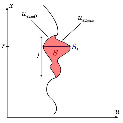
Figure 1: An avalanche in $d=1$.

The aim of this paper is to calculate further observables for the BFM which contain information about local properties, such as the joint density of global and local avalanches, and the distribution of extensions. We consider various protocols, where the interface is either driven uniformly in space or at a single point; in the latter case we identify new critical exponents. We study avalanches following a kick, i.e. a step in the driving force.

The article is structured as follows: In section II we recall the definition of the BFM and of the main avalanche observables, together with the general method to obtain them from the instanton equation. Section III starts by recalling the calculation of the distributions of the global size (total swept area) $S$ and of the local jump size $S_{r}$ of an avalanche, for an arbitrary kick amplitude. In Section III.3 we extend this calculation to the joint density $\rho(S_{r},S)$ of local and global size for single avalanches, i.e. in the limit of an infinitesimal kick. In Section IV we study the case of an interface driven at a single point. When the force at this point is imposed, we find a new exponent $\tau_{0}=5/3$ for the PDF of the local jump $S_{0}$ at that point. When the local displacement is imposed, we find a new exponent $\tau=7/4$ for the PDF of the global size $S$. In Section V we show that the extension $\ell$ of a single avalanche along one internal direction (i.e. the total length in $d=1$) is finite; we calculate its distribution, following either a local or a global kick. In all cases it exhibits a divergence $P(\ell)\sim\ell^{-3}$ at small $\ell$, with the same prefactor. All these exponents can be found in Table 1. Finally, in Section VI we study the position of the interface, which is a non-stationary process. We explain how the Larkin and BFM roughness exponents emerge from the dynamics. Most of our results are tested in a numerical simulation of the equation of motion in $d=1$.

Driving protocol	Observable	Exponent
any force kick	global size $S$	$\tau=3/2$
uniform force kick	local size $S_{0}$	$\tau_{0}=4/3$
uniform force kick	$S_{0}$ at fixed $S$	$\tau_{0}=2/3$
localized force kick	local size $S_{0}$	$\tau_{0}=5/3$
local displacement imposed	global size $S$	$\tau=7/4$
any force kick	extension $\ell$	$\kappa=3$

Table 1: Summary of small-scale exponents for different distributions in the Brownian-Force Model, depending on the observable and the driving protocol.

The technical parts of the calculations are presented in Appendices A to J, together with general material about Airy, Weierstrass and Elliptic functions. A short presentation of the numerical methods is also included.

Finally note a complementary recent study of the BFM, where the joint PDF of the local avalanche size at all points was obtained. From that, the spatial shape of an avalanche in the limit of large aspect ratio $S/\ell^{4}$ was derived ThieryLeDoussalWiese2015 .

II Avalanche observables of the BFM

II.1 The Brownian Force Model

In this paper, we study the Brownian Force Model (BFM) in space dimension $d$, defined as the stochastic differential equation (in the Ito sense) :

$$\eta\partial_{t}\dot{u}_{xt}=\nabla_{x}^{2}\dot{u}_{xt}+\sqrt{2\sigma\dot{u}_{xt}}\,\xi_{xt}+m^{2}(\dot{w}_{xt}-\dot{u}_{xt})\ .$$ (1)

This equation models the overdamped time evolution, with friction $\eta$, of the velocity field $\dot{u}_{xt}\geq 0$ of an interface with internal coordinate $x\in\mathbb{R}^{d}$; the space-time dependence is denoted by indices $\dot{u}(x,t)\equiv\dot{u}_{xt}$. It is the sum of three contributions:

• short-ranged elastic interactions,

• stochastic contributions from a disordered medium, where $\xi$ is a unit Gaussian white noise (both in $x$ and $t$) :

  $$\overline{\xi_{xt}\xi_{x^{\prime}t^{\prime}}}=\delta^{d}\!(x-x^{\prime})\,\delta(t-t^{\prime}),$$ (2)

• a confining quadratic potential of curvature $m$, centered at $w_{xt}$, acting as a driving.

The driving velocity is chosen positive, $\dot{w}_{xt}\geq 0$, a necessary condition for the model to be well defined, as it implies that $\dot{u}_{xt}\geq 0$ at all $t>0$ if $\dot{u}_{xt=0}\geq 0$.

Equation (1), taken here as a definition, can also be derived from the equation of motion of an elastic interface, parameterized by a position field (displacement field) $u_{xt}$ in a quenched random force field $F(u,x)$,

$$\eta\partial_{t}u_{xt}=\nabla_{x}^{2}u_{xt}+F\!\left(u_{xt},x\right)+m^{2}(w_{xt}-u_{xt})\ .$$ (3)

The random force field is a collection of independent one-sided Brownian motions in the $u$ direction with correlator

$$\overline{F(u,x)F(u^{\prime},x^{\prime})}=2\sigma\delta^{d}(x-x^{\prime})\min(u,u^{\prime})\ .$$ (4)

Taking the temporal derivative $\partial_{t}$ of Eq. (3), and assuming forward motion of the interface, one obtains Eq. (1) for the velocity variable $\partial_{t}u_{xt}\equiv\dot{u}_{xt}$ (we use indifferently $\partial_{t}$ or a dot to denote time derivatives). The fact that the equation for the velocity is Markovian even for a quenched disorder is remarkable and results from the properties of the Brownian motion.

Details of the correspondence are given in DobrinevskiLeDoussalWiese2011b ; LeDoussalWiese2012a where subtle aspects of the position theory, and its links to the mean-field theory of realistic models of interfaces in short-ranged disorder via the Functional Renormalisation Group (FRG) are discussed. In the last section of this paper we will mention some properties of the position theory of the Brownian force model.

II.2 Avalanches observables and scaling

The BFM (1) allows to study the statistics of avalanches as the dynamical response of the interface to a change in the driving. We consider solutions of (1) as a response to a driving of the form

$$\dot{w}_{xt}=\delta w_{x}~{}\delta(t)\,\,,\,\,\delta w_{x}\geq 0\,\,,\,\,\delta w=L^{-d}\int_{x}\delta w_{x}>0\ .$$ (5)

The initial condition is

$$\dot{u}_{xt=0}=0\ .$$ (6)

This solution describes an avalanche which starts at time $t=0$ and ends when $\dot{u}_{xt}=0$ for all $x$. The time at which the avalanche ends, also called avalanche duration, was studied in DobrinevskiPhD and its distribution given in various situations.

Within the description (3), i.e. in the position theory, it corresponds to an interface pinned, i.e. at rest in a metastable state at $t<0$, it is submitted at $t=0$ to a jump in the total applied force $m^{2}\delta w$. More precisely, the center of the confining potential jumps at $t=0$ from $w_{x}$ (where it was for $t<0$) to $w_{xt=0^{+}}=w_{x}+\delta w_{x}$ (where it stays for all $t>0$). As a consequence, the interface moves forward (since $\delta w_{x}\geq 0$) up to a new metastable state. This is represented in figure 1, where $u_{xt=0}$ is the initial metastable state and $u_{xt=\infty}$ is the new metastable state at the end of the avalanche. In fact, as we will see from the distribution of avalanche durations, the new metastable state is reached almost surely in a finite time. For details on these metastable states and the system’s preparation see DobrinevskiLeDoussalWiese2011b ; LeDoussalWiese2012a .

We now discuss the avalanche observables at the center of this paper. They can be computed from the solution of (1) given (5) and (6); they are represented in figure 1 for a more visual definition in the case $d=1$.

• Global size of the avalanche:

  $$S=\int_{x\in\mathbb{R}^{d}}\int_{0}^{\infty}\dot{u}_{tx}\,dt\ .$$ (7)

  This is the total area swept by the interface during the avalanche.

• Local size of the avalanche:

  $$S_{r}=m^{-1}\int_{x\in\{r\}\times\mathbb{R}^{d-1}}\int_{0}^{\infty}\dot{u}_{tx}\,dt\ .$$ (8)

  This is the size of the avalanche localized on a hyperplane, where one of the internal coordinates is $r$; the factor $m^{-1}$ allows to express $S$ and $S_{r}$ using the same units (see below). In $d=1$ this yields $S_{r}=m^{-1}\int_{0}^{\infty}\dot{u}_{tr}\,dt$, i.e. the transversal jump at the point $r$ of the interface. For $d>1$ the variable $r$ is still one-dimensional, and $S_{r}$ the total displacement in a hyperplane of the interface.

• Avalanche extension:

  For $d=1$, the extension (denoted $\ell$) of an avalanche is the lenght of the part of the interface which (strictly) moves during the avalanche. The generalisation to avalanches of a $d$-dimensional interface is done with the definition

  $$\ell=\int_{-\infty}^{\infty}dr~{}\theta(S_{r}>0)\ ,$$ (9)

  where $\theta$ is the Heaviside function. Note that even for a $d$-dimensional interface, the extension $\ell$ is a unidimensional observable (cf. figure 2).

Note that

$$S_{r}>0\ \Leftrightarrow\ {\rm Supp}\bigcap\{r\}\times\mathbb{R}^{d-1}\neq\emptyset$$ (10)

where ${\rm Supp}$ denotes all the points of the interface moving during an avalanche (i.e. its support).

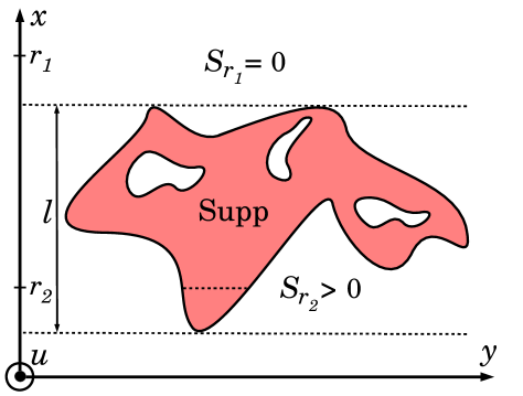
Figure 2: An avalanche in $d=2$; the transverse direction is orthogonal to the plane of the figure and the colored zone corresponds to the support of the avalanche.

We use natural scales (or units) to switch to dimensionless expressions, both for the (local and global) avalanche size $S_{m}$, as for the time $\tau_{m}$ expressed as

$$S_{m}=\frac{\sigma}{m^{4}}\ ,\qquad\tau_{m}=\frac{\eta}{m^{2}}\ .$$ (11)

The extension, a length in the internal direction of the interface, is expressed in units of $m^{-1}$. This is equivalent to setting $m=\sigma=\eta=1$. All expressions below, except explicit mention, are expressed in these units.

While $S_{m}$ is the large-size cutoff for avalanches, there is generically also a small-scale cutoff. As in the BFM the disorder is scale-invariant (by contrast with more realistic models with short-ranged smooth disorder), it is the increment in the driving $\delta w$ which sets the small-scale cutoff for the local and global size of avalanches. They scale as $\min(S)\sim\delta w^{2}$ (global size) and $\min(S_{r})\sim\delta w^{3}$ (local size).

Massless limit

There are cases of interest where the mass $m\to 0$. This can be defined from the equations of motion (1) and (3) with the changes

$$\begin{split}m^{2}(w_{xt}-u_{xt})&\to f_{xt}\\ m^{2}(\dot{w}_{xt}-\dot{u}_{xt})&\to\dot{f}_{xt}\ .\end{split}$$ (12)

In that case it is natural to consider driving with a given force $f_{xt}$, rather than by a parabola. The definition of the observables is the same except that the factor of $m^{-1}$ is not added in the definition (8). To bring $\sigma$ and $\eta$ to unity, we then define time in units of $\eta$ and displacements $u$ in units of $\sigma$. The results will still have an unfixed dimension of length. In some of them, the system size $L$ leads to dimensionless quantities (it also acts as a cutoff for large sizes, although we will not use this explicitly).

II.3 Generating functions and instanton equation

To compute the distribution of the observables presented above, we use a result from DobrinevskiLeDoussalWiese2011b ; LeDoussalWiese2012a which allows us to express the average over the disorder of generating functions (Laplace transforms) of $\dot{u}_{xt}$, solution of (1). In dimensionless units, this result reads

$$G[\lambda_{xt}]=\left\langle\exp\left(\int_{xt}\lambda_{xt}\dot{u}_{xt}\right)\right\rangle=e^{\int_{xt}\dot{w}_{xt}\tilde{u}_{xt}}\ .$$ (13)

Here $\langle\cdots\rangle$ denotes the average over disorder. $\tilde{u}$ is a solution of the differential equation (called instanton equation)

$$\partial_{x}^{2}\tilde{u}+\partial_{t}\tilde{u}-\tilde{u}+\tilde{u}^{2}=-\lambda_{xt}\ .$$ (14)

Since avalanche observables that we consider are integrals of the velocity field over all times (c.f. observable definitions above), the sources $\lambda_{xt}$ we need in (13) are time independent. Thus we only need to solve the space dependent, but time independent, instanton equation

$$\tilde{u}_{x}^{\prime\prime}-\tilde{u}_{x}+\tilde{u}^{2}_{x}=-\lambda_{x}\ .$$ (15)

The prime denotes derivative w.r.t $x$. In the massless case discussed above, the term $-\tilde{u}_{x}$ is absent, all other terms are identical.

The global avalanche size implies a uniform source in the instanton equation: $\lambda_{x}=\lambda$, while the local size implies a localized source $\lambda_{x}=\lambda\delta^{1}(x)$. To obtain information on the extension of avalanches, we need to consider a source localized at two different points in space, $\lambda_{x}=\lambda_{1}\delta(x-r_{1})+\lambda_{2}\delta(x-r_{2})$.

This instanton approach, which derives from the Martin-Siggia-Rose formulation of (1), allows us to compute exactly disorder averaged observables for any form of driving, by solving a “simple” ordinary differential equation, which depends on the observable we want to compute, i.e. on $\lambda_{xt}$, but not on the form of the driving $\dot{w}_{xt}$. For a derivation of (13) and (14) we refer to DobrinevskiLeDoussalWiese2011b .

III Distribution of avalanche size

III.1 Global size

As defined in (7) the global size of an avalanche is the total area swept by the interface. Its PDF was calculated in DobrinevskiLeDoussalWiese2011b ; LeDoussalWiese2011a ; LeDoussalWiese2012a and reads, in dimensionless units,

$$P_{\delta w}(S)=\frac{\delta\hat{w}}{2\sqrt{\pi}S^{\frac{3}{2}}}e^{-\frac{(S-\delta\hat{w})^{2}}{4S}}\ .$$ (16)

Here $\delta\hat{w}=L^{d}\delta w$. This result does not depend on the spatial form of the driving (it can be localized, uniform, or anything in between), as long as it is applied as a force on the interface. Driving by imposing a specific displacement at one point of the interface is another interesting case that leads to a different behavior, see Section IV.2.

We can test this against a direct numerical simulation of the equation of motion (1). There is excellent agreement over 5 decades, with no fitting parameter, see Fig. 3.

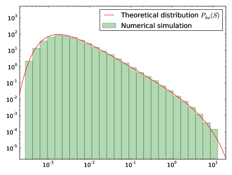
Figure 3: Green histogram : global avalanche-size distribution from a direct numerical simulation of a discretized version of Eq. (1) with parameters : $N=1024,m=0.01,df=m^{2}\delta w=1$ and $dt=0.05$. Red line : theoretical result given in Eq. (16). For details about the simulation see appendix H.

Avalanches have the property of infinite divisiblity, i.e. they are a Levy process. This can be written as an equality in distribution, i.e. for probabilities,

$$P_{\delta w_{1}}*P_{\delta w_{2}}\overset{d}{=}P_{\delta w_{1}+\delta w_{2}}\ .$$ (17)

It implies that we can extract from the probability distribution (16) the single avalanche density per unit $\delta w$ that we denote $\rho(S)$ and which is defined as

$$P_{\delta w}(S)\underset{\delta\hat{w}\ll 1}{\simeq}\delta w\,\rho(S)\ .$$ (18)

This avalanche density contains the same information as the full distribution (16); its expression is

$$\rho(S)=\frac{L^{d}}{2\sqrt{\pi}S^{\frac{3}{2}}}e^{-\frac{S}{4}}\sim S^{-\tau}\ .$$ (19)

It is proportional to the system volume since avalanches occur anywhere along the interface. It defines the avalanche exponent $\tau=\frac{3}{2}$ for the BFM. Due to the divergence when $S\rightarrow 0$ it is not normalizable (it is not a PDF), but as the interface follows on average the confining parabola, it has the following property

$$\int_{0}^{\infty}\!\!\!dS\,S\rho(S)=L^{d}\ .$$ (20)

In this picture, typical, i.e. almost all avalanches are of vanishing size, $S\approx 0$, or more precisely $S\leq\delta\hat{w}^{2}$, but moments of avalanches are dominated by non-typical large avalanches (of order $S_{m}$).

III.2 Local size

We now investigate the distribution of local size $S_{r}$ as defined in Eq. (8). We have to specify the form of the kick; we start with one uniform (in $x$): $\delta w_{x}=\delta w$ for all $x\in\mathbb{R}$. In this case the system is translationnaly invariant, and we can choose $r=0$, as any local size will have the same distribution.

The distribution of $S_{0}$ is obtained by solving Eq. $\eqref{instanton}$ with the source $\lambda_{x}=\lambda\delta(x)$, and then computing the inverse Laplace transform with respect to $\lambda$ of $G(\lambda)=\exp(\delta w\int_{x}\tilde{u}^{\lambda})$, where $\tilde{u}^{\lambda}$ is the instanton solution (depending on $\lambda$). This has been done in LeDoussalWiese2012a ; the final result is

$$\begin{split}\!\!P_{\delta w}(S_{0})&=\frac{2\times 3^{\frac{1}{3}}}{S_{0}^{\frac{4}{3}}}e^{6\delta\hat{w}}\delta\hat{w}\,\text{Ai}\!\left(\left(\frac{3}{S_{0}}\right)^{\!\frac{1}{3}}(S_{0}+2\delta\hat{w})\right)\\ &\simeq_{\delta\hat{w}\ll 1}\delta w\frac{2L^{d-1}}{\pi S_{0}}\text{K}_{\frac{1}{3}}\!\left(\frac{2S_{0}}{\sqrt{3}}\right)\ .\end{split}$$ (21)

Here $\delta\hat{w}=L^{d-1}\delta w$, Ai is the Airy function, and K the Bessel function. We use that $\text{Ai}(x)=\frac{1}{\pi}\sqrt{\frac{x}{3}}K_{1/3}(\frac{2}{3}x^{3/2})$ for $x>0$. This distribution has again the property of infinite divisibility, which is far from obvious on the final results but, can be checked numerically.

The small-$\delta w$ limit defines the density per unit $\delta w$ of the local sizes of a “single avalanche”, which is given by

$$\begin{split}\rho(S_{0})&=\frac{2L^{d-1}}{\pi S_{0}}\,\text{K}_{\frac{1}{3}}\!\!\left(\frac{2S_{0}}{\sqrt{3}}\right)\\ &\simeq_{S_{0}\ll 1}L^{d-1}\frac{\sqrt[6]{3}\,\Gamma(1/3)}{\pi{S_{0}}^{4/3}}\sim S_{0}^{-\tau_{\phi}}\ .\end{split}$$ (22)

Its small-size behavior defines the local size exponent $\tau_{\phi}=\frac{4}{3}$ for the BFM.

The distribution (21), or the density (22), can be compared to the results of direct numerical simulations of the BFM, and the agreement is very good over 7 decades, without any fitting parameter, c.f. Fig. 4.

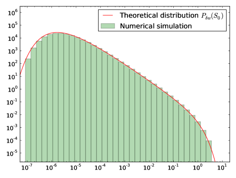
Figure 4: Green histogramm: Local avalanche-size distribution from a direct numerical simulation of a discretized version of (1)with parameters $N=1024,m=0.01,df=m^{2}\delta w=1$, and $dt=0.05$. Red line: the theoretical result given in Eq. (21). For details about the simulation see appendix H.

Another interesting property is that the tail of large local sizes behaves as $\rho(S_{0})\simeq_{S_{0}\gg 1}S_{0}^{-3/2}e^{-2S_{0}/\sqrt{3}}$, i.e. with the same power-law exponent in the pre-exponential factor as the global size.

III.3 Joint global and local size

We now extend these results with a new calculation of the joint density of local and global sizes. Consider $P_{\delta w}(S_{0},S)$, the joint PDF of local size $S_{0}$ and global size $S$, following a uniform kick $\delta w$. For arbitrary $\delta w$ it does not admit a simple explicit form (see Appendix D). We thus again consider the “single avalanche” limit $\delta w\rightarrow 0$. It defines the joint density $\rho(S,S_{0})$, via $P_{\delta w}(S_{0},S)\simeq\delta w\,\rho(S_{0},S)$, which we now calculate. Equivalently one can consider the conditional probability $P_{\delta w}(S_{0}|S)$ of the local size, given that the global size is $S$. In the limit $\delta w\to 0$ these two objects are related by

$$P_{0^{+}}\!(S_{0}|S)=\frac{\rho(S_{0},S)}{\rho(S)}\ ,$$ (23)

where $\rho(S)$ is given in Eq. (19); the two factors of $\delta w$ cancel. For simplicity we discuss the result for $P_{0^{+}}\!(S_{0}|S)$. While both $\rho(S)$ and $\rho(S_{0},S)$ are not probabilities, i.e. they cannot be normalized to one, we will show that the conditional probability $P_{0^{+}}\!(S_{0}|S)$ is well-defined, and normalized to unity.

A natural decomposition of this conditional PDF is

$$P_{0^{+}}\!(S_{0}|S)=\hat{P}_{0^{+}}\!(S_{0}|S)+\delta(S_{0})\left(1-\int_{u>0}\!\!\!\hat{P}_{0^{+}}\!(u|S)\right)\ .$$ (24)

The first term is the smooth part defined for $S_{0}>0$ which comes from the avalanches containing the point $r=0$. The second term arises from all avalanches which do not contain the point $r=0$. This term contains a substraction so that the total probability is normalized to unity, $\int_{S_{0}}P_{0^{+}}(S_{0}|S)=1$, as it should be.

The smooth part is calculated using the instanton-equation approach. The details are given Appendix D. The final result takes the scaling form

$$\hat{P}_{0^{+}}\!(S_{0}|S)=\frac{1}{L}{4\times 3^{2\over 3}\over S_{0}^{2\over 3}}e^{-\frac{2}{3}\alpha^{3}}\Big{[}\alpha\,\text{Ai}\big{(}\alpha^{2}\big{)}-\text{Ai}^{\prime}\big{(}\alpha^{2}\big{)}\Big{]}$$ (25)

with

$$\alpha:={3^{2\over 3}S_{0}^{4\over 3}\over S}\ .$$ (26)

The factor $1/L$ is natural since only a fraction of order $1/L$ of avalanches contains the point ${r=0}$. As written, this smooth part is not normalized. Its integral is equal to the probability $p$ that the point $S_{0}$ has moved (i.e. $S_{0}>0$) during an avalanche, for which we find

$$p:=\int_{0}^{\infty}\!\!\!dS_{0}\,\hat{P}_{0^{+}}(S_{0}|S)=\frac{S^{\frac{1}{4}}}{L}\frac{3\Gamma\!\left({1\over 4}\right)}{\sqrt{\pi}}\ .$$ (27)

The scaling of this probability with size shows that in a single avalanche only a finite portion of the interface is moving. If we assume statistical translational invariance we deduce that

$$p=\langle\ell\rangle_{S}/L\ ,$$ (28)

where $\ell$ is the extension defined in (9), and $\langle\ell\rangle_{S}$ its mean value conditioned to the global size $S$. Hence we deduce that

$$\langle\ell\rangle_{S}=\frac{3\Gamma\!\left({1\over 4}\right)}{\sqrt{\pi}}S^{\frac{1}{4}}\ .$$ (29)

In the following sections we will in fact calculate the PDF of the extension $\ell$.

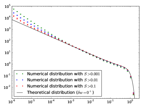
Figure 5: Distribution of $\alpha$, defined in Eq. (26), from numerical simulations ($N=1024,m=0.02,\delta w=10,dt=0.01$). This is compared to the theoretical prediction (33). Keeping only large-size avalanches, this converges (without any adjustable parameter) to the $\delta w=0^{+}$ result.

By dividing by $p$, we can now define a genuine normalized PDF for $S_{0}$, $\tilde{P}_{0^{+}}\!(S_{0}|S)$, conditioned to both $S$ and $S_{0}>0$, so that the decomposition (24) becomes

$$P_{0^{+}}\!(S_{0}|S)=p\,\tilde{P}_{0^{+}}\!(S_{0}|S)+\delta(S_{0})(1-p)\ .$$ (30)

Explicitly

$$\tilde{P}_{0^{+}}\!(S_{0}|S)=\frac{4\sqrt{\pi}e^{-\frac{2}{3}\alpha^{3}}}{3^{1\over 3}\Gamma\!\left(\frac{1}{4}\right)S_{0}^{2\over 3}S^{\frac{1}{4}}}\Big{[}\alpha\,\text{Ai}\big{(}\alpha^{2}\big{)}-\text{Ai}^{\prime}\big{(}\alpha^{2}\big{)}\Big{]}\ ,$$ (31)

with $\alpha$ defined in Eq. (26). It is now normalized to unity, $\int_{S_{0}>0}\tilde{P}_{0^{+}}(S_{0}|S)=1$. One sees that the typical local size scales as $S_{0}\sim S^{3/4}$. Computing the first moment we find its conditional average to be $\langle S_{0}\rangle_{S,S_{0}>0}=\frac{\sqrt{\pi}}{3\Gamma\left(1/4\right)}S^{3/4}$. Its PDF has two limiting behaviors,

$$\tilde{P}_{0^{+}}\!(S_{0}|S)\simeq\left\{\begin{array}[]{ll}\dfrac{e^{-\frac{12S_{0}^{4}}{S^{3}}}}{\Gamma(\frac{5}{4})S^{\frac{3}{4}}}&\text{ for }S_{0}\gg S^{\frac{3}{4}}\\ \dfrac{\sqrt{\pi}}{3^{\frac{2}{3}}\Gamma(\frac{1}{3})\Gamma(\frac{5}{4})S_{0}^{\frac{2}{3}}S^{\frac{1}{4}}}&\text{ for }S_{0}\ll S^{\frac{3}{4}}\ .\end{array}\right.$$ (32)

The first one shows that the probability of avalanches which are “peaked” at $r=0$ decays very fast. The second shows an integrable divergence at small $S_{0}$ with an exponent $2/3$. Comparing, for instance, with the behavior of the local size density (22), we see that conditioning on $S$ yields a rather different behavior and exponent.

It is interesting to note that changing variables in Eq. (31) from $S_{0}$ to $\alpha$, defined in (26), gives

$$\tilde{P}_{0^{+}}\!(\alpha|S)=\frac{\sqrt{3\pi}e^{-\frac{2}{3}\alpha^{3}}}{\Gamma\!\left(\frac{1}{4}\right)\alpha^{\frac{3}{4}}}\Big{[}\alpha\,\text{Ai}\big{(}\alpha^{2}\big{)}-\text{Ai}^{\prime}\big{(}\alpha^{2}\big{)}\Big{]}\ ,$$ (33)

which is now independant of $S$, and thus easier to test numerically as it does not require any conditionning. Figure 5 shows the agreement of these predictions with numerical simulations, in the limit of large $S$ which is equivalent to $\delta w=0^{+}$ as used in the theoretical derivation.

III.4 Scaling exponents

Let us now discuss the various exponents obtained until now. They are consistent with the usual scaling arguments for interfaces. If an avalanche has an extension of order $\ell$ (in the codirection of the hyperplane over which the local size is calculated), the transverse displacement scales as $u\sim\ell^{\zeta}$. Here the roughness exponent $\zeta$ for the BFM with SR elasticity is

$$\zeta_{{\rm BFM}}=4-d\ .$$ (34)

The avalanche exponent for the global size follows the Narayan-Fisher (NF) prediction NarayanDSFisher1993a

$$\tau=2-\frac{2}{d+\zeta}~{}\stackrel{{\scriptstyle\rm BFM}}{{-\!\!\!\longrightarrow}}~{}\frac{3}{2}\ .$$ (35)

The global size then scales as $S\sim\ell^{d+\zeta}$, since all $d$ internal directions are equivalent, and the transverse response scales with the roughness exponent $\zeta$. In turn this gives $\ell\sim S^{1\over d+\zeta}$. In the BFM with SR elasticity this leads to $\ell\sim S^{1/4}$ as found above.

Similarly, the local size, defined here as the avalanche size inside a $d_{\phi}$-dimensionel subspace, is $S_{0}\sim\ell^{d_{\phi}+\zeta}$ , leading to a generalized NF value $\tau_{\phi}=2-\frac{2}{d_{\phi}+\zeta}$. In the BFM we have focused on the case $d_{\phi}=d-1$ (i.e. the subspace is an hyperplane), hence $d_{\phi}+\zeta=3$ and the local size exponent becomes $\tau_{\phi}=4/3$. It also implies $S_{0}\sim\ell^{3}$, hence $S_{0}\sim S^{3/4}$ as found above.

IV Driving at a point: avalanche sizes

Here we briefly study avalanche sizes for an interface driven only in a small region of space, e.g. at a point. There are two main cases:

• the local force on the point is imposed, which in our framework means to consider a local kick $\delta w_{x}=\delta w\,\delta(x)$. In the massless setting it amounts to use $f_{x}=\delta f\,\delta(x)$,

• the displacement $u_{x=0,t}$ of one point of the interface is imposed.

As we now see this leads to different universality classes and exponents.

IV.1 Imposed local force

Consider an avalanche following a local kick at $x=0$, i.e. $\delta w_{x}=\delta w_{0}\delta(x)$.

In the BFM the distribution of the global size of an avalanche does not depend on whether the kick is local in space or not. One still obtains LeDoussalWiese2012a the global-size distribution as given in Eq. (16) with $\delta\hat{w}=\int_{x}\delta w_{x}=\delta w_{0}$.

The distribution of the local size at the point of the kick is more interesting. The calculation is performed in Appendix C.2. For simplicity we restrict to $d=1$, the general case can be obtained as above by inserting factors of $L^{d-1}$. The full result for the PDF, $P_{\delta w_{0}}\!(S_{0})$, is given in (C.2) and is bulky. In the limit $\delta w_{0}\to 0$ it simplifies. Noting $P_{\delta w_{0}}\!(S_{0})\simeq\delta w_{0}\rho(S_{0})$, the corresponding local-size density becomes

$$\rho(S_{0})=-\frac{1}{3^{1/3}S_{0}^{5/3}}\text{Ai}^{\prime}\!\left(3^{1/3}S_{0}^{2/3}\right)\ .$$ (36)

At small $S_{0}$, or equivalently in the massless limit at fixed $\delta f_{0}=m^{2}\delta w_{0}$, it diverges as

$$\rho(S_{0})\underset{S_{0}\ll 1}{\simeq}\frac{S_{0}^{-5/3}}{3^{2/3}\Gamma(1/3)}\sim S_{0}^{-\tau_{0,{\rm loc.driv.}}}\ .$$ (37)

This leads to a new avalanche exponent

$$\tau_{0,{\rm loc.driv.}}=\frac{5}{3}\ .$$ (38)

The cutoff at small size is given by the driving, $S_{0}\sim\delta w_{0}^{3/2}$. At large $S_{0}$ the PDF is cut by the scale $S_{m}\equiv 1$ and decays as

$$\rho(S_{0})\underset{S_{0}\gg 1}{\simeq}\frac{S_{0}^{-3/2}}{2\sqrt{\pi}3^{1/4}}e^{-2S_{0}/\sqrt{3}}\ .$$ (39)

IV.2 Imposed displacement at a point

We analyze the problem in the massless case. To impose the displacement at point $x=0$ we replace in the equation of motion (1) and (3), $m^{2}\to m^{2}\delta(x)$. Hence there is no global mass, but a local one to drive the interface at a point. To impose the displacement, we consider the limit $m^{2}\to\infty$. In that limit $u_{x=0,t}=w_{0,t}$, and the local size of the avalanche $S_{0}$ is equal to $\delta w_{0}$.

While the local size $S_{0}$ is fixed by the driving, we can calculate the distribution of global sizes. It is obtained in Appendix E using an instanton equation with a Dirac mass term. It can be mapped onto the same instanton equation as studied for the joint PDF of local and global sizes. The Laplace-transform of the result for the PDF is given in Eq. (136). Its small-driving limit, i.e. the density, is

$$\rho(S)=\frac{\sqrt{3}}{\Gamma(1/4)S^{7/4}}\sim S^{-\tau_{\rm loc.driv.}}$$ (40)

with a distinct exponent

$$\tau_{\rm loc.driv.}=\frac{7}{4}\ .$$ (41)

V Distribution of avalanche extensions

In this section we study the distribution of avalanche extensions. In the BFM they can be calculated analytically. We start by recalling standard scaling arguments.

V.1 Scaling arguments for the distribution of extensions

As mentioned in the last section, we expect that the global size $S$ and the extension $\ell$ of avalanches are related by the scaling relation

$$S\sim\ell^{d+\zeta}$$ (42)

in the region of small avalanches $S\ll S_{m}$ (in dimensionfull units). From the definition of the avalanche-size exponent

$$P(S)\sim S^{-\tau}$$ (43)

and using the change of variables $P(S)dS=P(\ell)d\ell$ we find

$$P(\ell)\sim\ell^{-\kappa}\,\text{ with }\,\kappa=1+(\tau-1)(d+\zeta)\ .$$ (44)

Using the value for $\tau$ from the NF relation (35) we obtain

$$\tau=2-\frac{2}{d+\zeta}\ .$$ (45)

For SR elasticity, this yields

$$\kappa=d+\zeta-1\ .$$ (46)

The prediction for the BFM is that $\zeta_{\rm BFM}=4-d$ and $\tau_{\rm BFM}=3/2$, which leads to

$$\kappa_{\rm BFM}=3$$ (47)

in all dimensions. We will now check this prediction from the scaling relations with exact calculations on the BFM model in $d=1$.

V.2 Instanton equation for two local sizes

If we want to investigate the joint distribution of two local sizes at points $r_{1}$ and $r_{2}$, we need to solve the instanton equation with two local sources,

$$\tilde{u}^{\prime\prime}_{x}-\tilde{u}_{x}+\tilde{u}^{2}_{x}=-\lambda_{1}\delta(x-r_{1})-\lambda_{2}\delta(x-r_{2})\ .$$ (48)

This solution is difficult to obtain for general values of $\lambda_{1}$ and $\lambda_{2}$. Nevertheless $\lambda_{1,2}\rightarrow-\infty$ is an interesting solvable limit, and sufficient to compute the extension distribution. Let us denote by $\tilde{u}_{r_{1},r_{2}}(x)$ a solution of Eq. (48) with $r_{1}<r_{2}$ in this limit $\lambda_{1,2}\rightarrow-\infty$. It allows to express the probability that two local sizes in an avalanche following an arbitrary kick $\delta w_{x}$ equal $0$,

$$\begin{split}\mathbb{P}_{\delta w_{x}}(S_{r_{1}}=0&,S_{r_{2}}=0)\\ &=\exp\left(\int_{x\in\mathbb{R}^{d}}\delta w_{x}\,\tilde{u}_{r_{1},r_{2}}(x)\right)\ .\end{split}$$ (49)

We further restrict for simplicity to the massless case, i.e. without the linear term $\tilde{u}_{x}$ in Eq. (48). One easily sees from the latter equation that $\tilde{u}_{r_{1},r_{2}}$ takes the scaling form

$$\tilde{u}_{r_{1},r_{2}}(x)=\frac{1}{(r_{1}-r_{2})^{2}}\,f\!\left(\frac{2x-r_{1}-r_{2}}{2(r_{2}-r_{1})}\right)\ .$$ (50)

The function $f(x)$ is solution of

$$f^{\prime\prime}(x)+f(x)^{2}=0\ .$$ (51)

It diverges at $x=\pm\frac{1}{2}$, vanishes at $x\to\pm\infty$ and is negative everywhere: $f(x)\leq 0$. As $\delta w_{x}\geq 0$, the latter is a necessary condition s.t. the probability (49) is bounded by one.

In the interval $x\in]-\frac{1}{2},\frac{1}{2}[$, the scaling function $f(x)$ can be expressed in terms of the Weierstrass $\mathcal{P}$-function, see (177),

$$f(x)=-6\,\mathcal{P}\!\left(x+\frac{1}{2};g_{2}=0;g_{3}=\frac{\Gamma(1/3)^{18}}{(2\pi)^{6}}\right)\ .$$ (52)

The value of $g_{3}>0$ is consistent with the required period $2\Omega=1$, see (174). Note from Appendix I that there is another solution of the form (52) with $g_{3}=-\Big{(}2\sqrt{\pi}\frac{\Gamma(1/3)}{4^{\frac{1}{3}}\Gamma(5/6)}\Big{)}^{6}<0$ which violates the condition $f(x)\leq 0$, hence is discarded. For $|x|\geq 1/2$, the function $f(x)$ reads

$$f(x)=-\frac{6}{(|x|-1/2)^{2}}\ .$$ (53)

One property of the solution $\tilde{u}_{r_{1},r_{2}}(x)$ is that it diverges as $\sim(x-r_{1,2})^{-2}$ when $x\approx r_{1,2}$. There are thus two cases:

(i) - the driving $\delta w_{x}$ is non-zero at one of these points, or vanishes too slowly near this point (e.g. only linearly or slower). Then the integral in (49) is not convergent, equal to $-\infty$, which implies

$$\mathbb{P}_{\delta w_{x}}(S_{r_{1}}=0,S_{r_{2}}=0)=0\ .$$

This means that the avalanche contains surely at least one of the points $r_{1}$ or $r_{2}$.

(ii) - If $\delta w_{x}$ vanishes fast enough, for example if $\delta w_{x}$ is localised away from $x=\pm r_{1,2}$ (e.g $\delta w_{x}=\delta w\delta(x-y)$ for some $y\in\mathbb{R}\backslash\{r_{1},r_{2}\}$), the probablity (49) becomes non trivial.

V.3 Avalanche extension with a local kick

We now consider a local kick centered at $x=0$, i.e. $w_{x}=\delta w_{0}\,\delta(x)$. If further $0<r_{1}<r_{2}$, then

$$\mathbb{P}_{\delta w_{0}}\!\left(S_{r_{1}}=0,S_{r_{2}}=0\right)=\mathbb{P}_{\delta w_{0}}\!\left(S_{r_{1}}=0\right)\ .$$ (54)

This comes from the fact that in the interval $x\in[-\infty,r_{1}]$, the solution $\tilde{u}_{r_{1},r_{2}}(x)$ is identical to the instanton solution with only one infinite source at $r_{1}$ (in other word, it does not “feel” the source in $r_{2}$). This shows for instance that the support of the avalanche is larger or equal than the set of points where the driving is non-zero.

This property also shows that avalanches are connected, i.e. it is impossible to draw a plane where the interface did not move between two moving parts of the interface. As a function of $r$ (which is one-dimensional), the support (i.e. the set of points where $S_{r}>0$) of an avalanche following a local kick at $x=0$ must be an interval. Since this interval contains $x=0$ we will write it as $[-\ell_{1},\ell_{2}]$ with $\ell_{1}>0$ and $\ell_{2}>0$. This allows to define the extension of an avalanche as $\ell=\ell_{1}+\ell_{2}$.

To calculate the joint PDF of $\ell_{1}$ and $\ell_{2}$ for a kick at $x=0$ we consider (49) with $r_{1}=-x_{1}<0<r_{2}=x_{2}$. Using the previous results about the instanton equation with two sources, and the fact that the interface model is translationaly invariant, we obtain the joint cumulative distribution for $\ell_{1}>0$ and $\ell_{2}>0$:

$$F_{\delta w_{0}}(x_{1},x_{2}):=\mathbb{P}_{\delta w_{0}}\left(\ell_{1}<x_{1},\ell_{2}<x_{2}\right)\ .$$ (55)

It can, for any $x_{1},x_{2}>0$, be expressed in terms of the function $f$ obtained in the preceding section,

$$\begin{split}F_{\delta w_{0}}(x_{1},x_{2})&=\mathbb{P}_{\delta w_{0}}\!\left(S_{r_{1}}=0,S_{r_{2}}=0\right)\\ &=\exp\!\left(\int_{x}\delta w_{0}\delta(x)\,\tilde{u}_{-x_{1},x_{2}}(x)\right)\\ &=e^{\delta w_{0}\frac{1}{(x_{1}+x_{2})^{2}}f\left(-\frac{x_{2}-x_{1}}{2(x_{1}+x_{2})}\right)}\end{split}\ .$$ (56)

Since the argument of $f$ is within the interval $]-\frac{1}{2},\frac{1}{2}[$ we must use the expression (52).

From this one can obtain several results. First taking $x_{2}\to\infty$ one obtains the PDF of $\ell_{1}$ alone,

$$\mathbb{P}_{\delta w}\left(\ell_{1}\right)=\frac{12\delta w}{\ell_{1}^{3}}e^{-\delta w\frac{6}{\ell_{1}^{2}}}\ .$$ (57)

A similar result holds for $\ell_{2}$.

In principle, one can now obtain the distribution of avalanches extensions

$$\mathbb{P}_{\delta w_{0}}\!\left(\ell\right)=\int_{0}^{\infty}\!\!\!\!d\ell_{1}\int_{0}^{\infty}\!\!\!\!d\ell_{2}\,\delta(\ell-\ell_{1}-\ell_{2})\partial_{\ell_{1}}\partial_{\ell_{2}}F_{\delta w_{0}}(\ell_{1},\ell_{2})$$ (58)

It has a rather complicated expression. Let us define in addition to the total length, the aspect ratio

$$k=\frac{\ell_{1}-\ell_{2}}{2(\ell_{1}+\ell_{2})}\quad,\quad-\frac{1}{2}<k<\frac{1}{2}\ .$$ (59)

Using a change of variables, we obtain the joint density of total extension and aspect ratio in the limit $\delta w_{0}\to 0$,

$$\rho\left(\ell,k\right) := \lim\limits_{\delta w_{0}\to 0}\frac{1}{\delta w_{0}}\mathbb{P}_{\delta w_{0}}\left(\ell,k\right)=\frac{R(k)}{\ell^{3}}\ ,\;$$ (60)

$$R(k) := 6f(k)+6kf^{\prime}(k)+\left(k^{2}-\frac{1}{4}\right)f^{\prime\prime}(k)\ .~{}~{}$$ (61)

The function $f(x)$ was defined in Eq. (52). While the probability as a function of $\ell$ decays as $\ell^{-3}$, the dependence on the aspect ratio is more complicated and plotted in figure 6. Note that in this expression $f(k)$ can be replaced by $f_{\rm reg}(k):=f(k)+\frac{6}{(k+\frac{1}{2})^{2}}+\frac{6}{(k-\frac{1}{2})^{2}}$, which is a regular function of $k$, vanishing at $k=\pm\frac{1}{2}$.

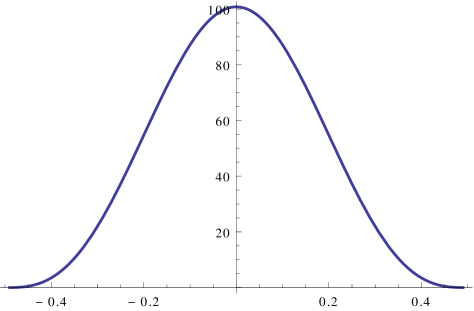
Figure 6: Decay amplitude $R(k)$ as a function of the aspect ratio $k$ involved in the joint density of $\ell$ and $k$, and defined in Eqs. (60) and (61).

Integration over $k$ gives

$$\rho\left(\ell\right) = \frac{B}{\ell^{3}}\qquad\text{ with }$$ (62)

$$B = 24+2\int_{-1/2}^{1/2}f_{\rm reg}(k)=8\sqrt{3}\pi\ .$$ (63)

V.4 Avalanche extension with a uniform kick

If a kick extends over the whole system, as e.g. a uniform kick $\delta w_{x}=\delta w$, the avalanche will have almost surely an infinite extension as the local size is non-zero everywhere,

$$\mathbb{P}_{\delta w}\left(S_{r}=0\right)=0\ \text{ for any }\,{r}\in\mathbb{R}\ .$$ (64)

However, in the limit of a small $\delta w$ which is also the limit of a “single avalanche”, we can recover the result for the distribution of extensions. This is consistent with the idea that “single avalanches” do not depend on the way they are triggered. These calculations allow to obtain the extension distribution without solving explicitly the instanton equation. (The use of elliptic integrals is in fact equivalent to the use of Weierstrass functions as solutions of the instanton equation, c.f. Appendix I).

We now focus on the following ratio of generating functions

$${\langle e^{\lambda_{1}s_{0}+\lambda_{2}s_{r}}\rangle\over\langle e^{\lambda_{1}s_{0}}\rangle\langle e^{\lambda_{2}s_{r}}\rangle}$$ (65)

in the limit $\lambda_{1},\lambda_{2}\rightarrow-\infty$. It compares the probability that both local sizes $s_{0}:=S_{0}$ and $s_{r}:=S_{r}$ are simultaneously $0$ to the product of the two probabilties that each one is $0$.

We can express this ratio, using the instanton-equation approach, as

$$\begin{split}\lim_{\lambda_{1},\lambda_{2}\rightarrow-\infty}&{\langle e^{\lambda_{1}s_{0}+\lambda_{2}s_{r}}\rangle\over\langle e^{\lambda_{1}s_{0}}\rangle\langle e^{\lambda_{2}s_{r}}\rangle}\\ =\exp\!\bigg{(}&\int_{x}\delta w_{x}\Big{[}\tilde{u}_{r}(x)-\tilde{u}_{\infty}(x)-\tilde{u}_{\infty}(x-r)\Big{]}\bigg{)}\end{split}$$ (66)

where $\tilde{u}_{r}:=\tilde{u}_{r_{1}=0,r_{2}=r}$. We denote by $\tilde{u}_{\infty}:=\tilde{u}_{r_{1}=0,r_{2}=\infty}$, the solution of the instanton equation with one source at $r=0$ and the other one at infinity. It is the same as the solution for only one source in $r=0$. The above expression is valid for any form of driving $\delta w_{x}$.

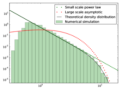
Figure 7: The distribution of extensions $\rho(\ell)$, as obtained from the elliptic integrals (144) and (145) (black line). The (straight) green dotted line is the small-$\ell$ asymptotics (V.4), whereas the (curved) red dotted line is the large-$\ell$ asymptotics (71). The numerical simulation (green histogram) is cut at small scale due to discretization effects.

We can now specify to the case of small and uniform driving $\delta w_{x}=\delta w$; the quantity of interest is then

$$Z(r)=\int_{x}\tilde{u}_{r}(x)-\tilde{u}_{\infty}(x)-\tilde{u}_{\infty}(x-r)\ .$$ (67)

While $\tilde{u}_{r}(x)$ is not integrable, $Z(r)$ is well defined as the two $\tilde{u}_{\infty}$ terms cancel precisely the two non-integrable poles located at $x=0$ and $x=r$.

Using that $\tilde{u}_{r}$ is a solution of Eq. (48), we can obtain an expression of $Z(r)$ as an elliptic integral, see Appendix F for details of the calculation. The formulas written there are for the massive case, but only allow to get an implicit expression for $Z(r)$. They however allow us to extract the small-scale behavior of the avalanche-extension distribution (equivalently the massless limit). For small $r$, the behavior of $Z(r)$ is

$$Z(r)\simeq\frac{4\sqrt{3}\pi}{r}\ .$$ (68)

To understand the connection with the avalanche extension, we need to get back to the interpretation of (65). Now that we have specified the kick to be uniform, the two averages of the denominator are independant of $r$, and act only as a normalization constants. The numerator, in the limit of $\lambda_{1,2}\rightarrow-\infty$, is the probability that both $s_{0}$ and $s_{r}$ are simultaneously equal to $0$. Deriving this two times w.r.t. $r$ (which lets the denominator invariant) gives the probability that the avalanche start in $x=0$ and end in $x=r$. Dividing by $\delta w$ and taking the limit $\delta w\to 0$ , we obtain the extension density in the limit of a single avalanche as

$$\rho(\ell) = \frac{1}{\delta w}\partial_{r}^{2}e^{\delta wZ(r)}|_{\delta w=0^{+},r=\ell}$$

$$= \partial_{r}^{2}\left.\tilde{Z}(r)\right\rvert_{r=\ell}\simeq\tilde{B}\ell^{-3}\,\text{ when }\,\ell\rightarrow 0$$

with

$$\tilde{B}=8\sqrt{3}\pi\ .$$ (70)

We recover here the $\ell^{-3}$ divergence for small $\ell$ of the extension of avalanches. Note that this calculation gives exactly the same prefactor as in Eq. (62), which confirms that we are studying the same object, namely a “single avalanche”.

Finally, in the massive case, one can also compute the tail of the extension distribution, resulting into (see Appendix F)

$$\rho(\ell)\simeq 72\,\ell e^{-\ell}\text{ when }\ell\rightarrow\infty\ .$$ (71)

VI Non-stationnary dynamics in the BFM

The easiest way to construct a position theory equivalent to the BFM model define in Eq. (1) is to consider the non-stationnary evolution of an elastic line in some specific quenched disorder,

$$\eta\partial_{t}u_{xt}=\nabla_{x}^{2}u_{xt}+F\left(u_{xt},x\right)+m^{2}(w_{xt}-u_{xt})\ .$$ (72)

Here the disorder has the correlations of independent one-sided Brownian motion

$$\overline{F(u,x)F(u^{\prime},x^{\prime})}=2\sigma\delta^{d}(x-x^{\prime})\min(u,u^{\prime})\ .$$ (73)

Consider the initial condition $u_{xt=0}=0$. We can then compute the correlation function of the position

$$u_{xt}=\int_{0}^{t}\dot{u}_{xs}\,ds$$

for a uniform driving $w_{t}=vt\,\theta(t)$, starting at $t=0$. The calculation is sketched in Appendix J. In dimensionless units and in Fourier space, the result reads

$$\langle u_{qt}u_{-qt}\rangle^{c} = v\Bigg{[}\frac{2q^{2}(t-1)+2t-5}{\left(q^{2}+1\right)^{3}}-\frac{4e^{-\left(q^{2}+1\right)t}}{q^{2}\left(q^{2}+1\right)^{3}}$$ (74)

$$+\frac{4e^{-t}}{q^{2}\left(2q^{2}+1\right)}+\frac{e^{-2\left(q^{2}+1\right)t}}{\left(q^{2}+1\right)^{3}\left(2q^{2}+1\right)}\Bigg{]}\ .~{}~{}~{}~{}~{}~{}~{}~{}$$

At large times, the displacement correlations behave as (restoring units)

$$\langle u_{qt}u_{-qt}\rangle^{c}\underset{t\rightarrow\infty}{\simeq}\frac{2\sigma vt}{(q^{2}+m^{2})^{2}}\ .$$ (75)

The $q$ dependence is similar to the so-called Larkin random-force model Larkin1970 , but with a time-dependent amplitude, i.e. the effective disorder is growing with time, which is natural given the correlations (73). The correlation of the position thus remains non-stationary at all times.

From Eq. (75) one obtains the correlations of the displacement in real space, still in the large-$t$ limit

$$\overline{(u_{xt}-u_{0t})^{2}} \simeq 2vt\int\frac{d^{d}q}{(2\pi)^{d}}\frac{1}{(q^{2}+m^{2})^{2}}(1-\cos qx)$$ (76)

$$\sim vt\times x^{2\zeta_{L}}$$

with $\zeta_{L}=(4-d)/2$ the Larkin roughness exponent. Note that the average displacement is $\overline{u_{xt}}=vt-\frac{1-e^{-m^{2}t}}{m^{2}}$ (see Appendix J ). Hence we see that the BFM roughness scaling $u\sim x^{4-d}$ is dimensionally consistent with the correlation at large times,

$$\overline{(u_{xt}-u_{0t})^{2}}\simeq 2~{}\overline{u_{xt}}~{}x^{4-d}\ .$$ (77)

This result, $\zeta=4-d=\varepsilon$, is in agreement with the FRG approch: the position theory of the BFM model is an exact fixed point for the flow equation of the FRG with a roughness exponent $\zeta=\varepsilon$, as discussed in LeDoussalWiese2011b ; DobrinevskiLeDoussalWiese2011b .

VII Conclusion

We presented a general investigation of the Brownian Force Model, using its exact solvability via the instanton equation in various settings. After reviewing the results and the calculations of LeDoussalWiese2008c ; LeDoussalWiese2011a ; DobrinevskiLeDoussalWiese2011b ; LeDoussalWiese2012a , we extended the study in several directions.

First, we computed observables containing information about the spatial structure of avalanches in the BFM: the joint density of $S$ and $S_{0}$ (or equivalently, the distribution of the local size $S_{0}$ at fixed total global size $S$), and the distribution of the extension $\ell$ of an avalanche. These distributions display power laws in their small-scale regime, which we recovered using scaling arguments, together with universal amplitudes.

We also extended the method to study new driving protocols relevant to distinct experimental setups. The derived results show new exponents for the small-scale behavior of the global avalanche-size distribution following a locally imposed displacement, and for the small-scale behavior of the local-size distribution following a localized kick.

Finally, we presented results for the non-stationary dynamics of the BFM, focusing on observables which exist only in the position theory, such as the roughness exponent. This explains why both the Larkin roughness and the BFM roughness (emerging from the FRG approach), play a role in this model, depending on whether the driving is stationary or not.

Appendix A Airy functions

We recall the definition of the Airy function:

$$\text{Ai}(z):=\int_{-\infty}^{\infty}\frac{dt}{2\pi}e^{i\frac{t^{3}}{3}+izt}\ .$$ (78)

The following formula is usefulfor $a\in\mathbb{R}^{*}$,

$$\Phi(a,b,c) = \int_{C}\frac{dz}{2i\pi}e^{a\frac{z^{3}}{3}+bz^{2}+cz}$$

$$= |a|^{-1/3}e^{\frac{2b^{3}}{3a^{2}}-\frac{bc}{a}}\text{Ai}\!\left(\frac{b^{2}}{|a|^{4/3}}-\frac{c~{}{\rm sgn}(a)}{|a|^{1/3}}\right)\ .$$

It can be obtained from (78), deforming the contour $C$, e.g. to $z=-\frac{b}{a}+i\mathbb{R}$.

Appendix B General considerations on the instanton equation

B.1 Sourceless equation

B.1.1 Massive case

It is useful to start with the simpler sourceless instanton equation

$$y^{\prime\prime}=y-y^{2}\ .$$ (80)

Here we denote by a prime the derivative with respect to $x$. It can be interpreted as the classical equation of motion of a particule (of mass $2$) in a potential $V(y)=-y^{2}+{2y^{3}\over 3}$, represented in Fig. 8. Multiplying by $y^{\prime}$ and integrating once, we obtain $y^{\prime}=\pm\sqrt{E-V(y)}$, where $E$ is a real integration constant equivalent to the total “energy” of the particle. Its phase-space diagram $(y,y^{\prime})$ is represented in Fig. 9.

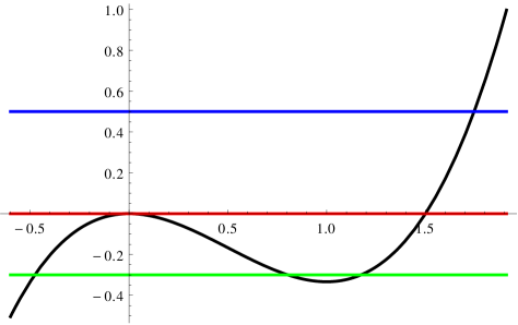
Figure 8: Representation of the potential energy $V(y)$ as a function of $y$, and lines of constant total energy, with $E=0$ in red, $E>0$ in blue and, $E<0$ in green.

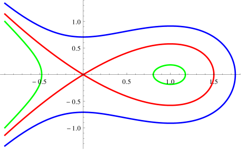
Figure 9: Phase-space diagram, i.e. trajectories represented with $y^{\prime}$ as a function of $y$. The case $E=0$ is in red, $E>0$ in blue and and $E<0$ in green. We can see that properties of the solution (periodicity, divergences, etc.) strongly depend on the value of $E$.

From figures 8 and 9, we see that:

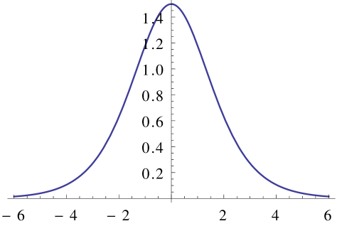
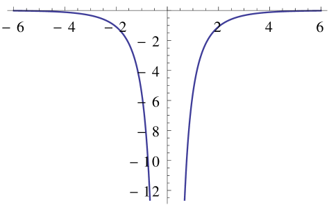
Figure 10: Solutions with energy $0$ of equation (80); left : $y^{+}(x)$, right : $y^{-}(x)$.

(i) - there is exactly one positive $E=0$ solution $y^{+}(x)$ defined for all $x\in\mathbb{R}$, up to a shift $x\to x+x_{0}$. It reads

$$\begin{split}&\int_{y^{+}(x)}^{3/2}\frac{dy}{\sqrt{y^{2}-\frac{2}{3}y^{3}}}=|x|\\ &\Leftrightarrow\;y^{+}\!(x)=\frac{3}{1+\cosh x}=\frac{3}{2}\bigg{[}1-\tanh^{2}\!\left(\frac{x}{2}\right)\bigg{]}\ .\end{split}$$ (81)

(ii) - There is exactly one negative $E=0$ (zero energy) solution $y^{-}(x)$ defined for all $x\in\mathbb{R}^{*}$, namely

$$\begin{split}&\int^{y^{-}\!(x)}_{-\infty}\!\!\!\frac{dy}{\sqrt{y^{2}-\frac{2}{3}y^{3}}}=|x|\\ &\Leftrightarrow\;y^{-}(x)=\frac{3}{1-\cosh x}=\frac{3}{2}\bigg{[}1-\coth^{2}\!\left(\frac{x}{2}\right)\bigg{]}\ .\end{split}$$ (82)

(iii) - There are two classes of solutions with $E\neq 0$. The first class is defined on an interval of finite length $r(E)$ with

$$r(E)=2\int^{t}_{-\infty}\frac{dy}{\sqrt{E+y^{2}-\frac{2}{3}y^{3}}}$$ (83)

where $t\neq 0$ denotes the smallest real root of $E=-t^{2}+\frac{2}{3}t^{3}$. This integral is convergent at large negative $y$ due to the cubic term, and also convergent near the root $y=t$ (for $E\to 0$ it diverges logarithmically). If one chooses $x=0$ as center of the interval, the solution $y(x)$ satisfies

$$\int^{t}_{y(x)}\frac{dy}{\sqrt{E+y^{2}-\frac{2}{3}y^{3}}}=|x|\ .$$ (84)

It diverges at both ends $x=\pm r(E)/2$. It is sometimes more convenient to choose $x=0$ as the endpoint of the interval $]0,r(E)[$. Then, for $x\in]0,r(E)[$ one has

$$\int^{y(x)}_{-\infty}\frac{dy}{\sqrt{E+y^{2}-\frac{2}{3}y^{3}}}=x\ .$$ (85)

Setting $y=\frac{1}{2}-z$, this can be rewritten as

$$\sqrt{6}\int_{\frac{1}{2}-y(x)}^{\infty}\frac{dz}{\sqrt{4z^{3}-3z+(1+6E)}}=x\ .$$ (86)

This gives, in terms of the Weirstrass elliptic function $\cal P$,

$$y(x)=\frac{1}{2}-{\cal P}\!\left(\frac{x}{\sqrt{6}};g_{2}=3,g_{3}=-1-6E\right)\ .$$ (87)

It diverges at $x=0$ and $x=r(E)$, and is the proper solution on the interval $]0,r(E)[$, see Appendix I.

The second class of solutions with $E\neq 0$ exists only for $-\frac{1}{3}<E<0$; these solutions are periodic on the whole real line. As can be seen from Figs. 8 and 9, $y(x)$ varies in a bounded and strictly positive interval. We will not discuss these solutions as they will not be needed below.

B.1.2 Massless case

Consider now the massless sourceless equation,

$$y^{\prime\prime}=-y^{2}\ .$$ (88)

The analysis is similar to the massive case discussed above with $V(y)=-\frac{2}{3}y^{3}$. Its solutions have the following properties:

(i) - there is no positive $E=0$ solution.

(ii) - There is only one negative $E=0$ solution $y^{-}(x)$ defined for all $x\in\mathbb{R}^{*}$,

$$\int^{y^{-}(x)}_{-\infty}\frac{dy}{\sqrt{-\frac{2}{3}y^{3}}}=|x|\Leftrightarrow y^{-}(x)=-\frac{6}{x^{2}}\ .$$ (89)

It can be obtained by considering the limit $x\ll 1$ in the solution (82).

(iii) - There is now only one class of solutions with $E\neq 0$ (the periodic ones have disappeared). They are defined on an interval of length $r(E)$. They have $E=\frac{2}{3}t^{3}$, hence $t=(3E/2)^{1/3}$ and

$$r(E) = 2\int^{t}_{-\infty}\frac{dy}{\sqrt{\frac{2}{3}t^{3}-\frac{2}{3}y^{3}}}$$ (90)

$$= \begin{cases}\sqrt{6\pi}\left(\frac{2}{3|E|}\right)^{\!1/6}\frac{\Gamma(1/3)}{\Gamma(5/6)}\,,\quad E>0\\ \sqrt{6\pi}\left(\frac{2}{3|E|}\right)^{\!1/6}\frac{2\Gamma(7/6)}{\Gamma(2/3)}\,,\;\;E<0\ .\end{cases}$$

The solution $y(x)$ satisfies for $x\in]0,r(E)[$

$$\int^{y(x)}_{-\infty}\frac{dy}{\sqrt{E-\frac{2}{3}y^{3}}}=x\ .$$ (91)

It can be expressed in terms of the Weirstrass function,

$$y(x)=-{\cal P}\!\left(\frac{x}{\sqrt{6}};g_{2}=0,g_{3}=-6E\right)\ .$$ (92)

It diverges at $x=0$ and $x=r(E)$. The periods are consistent with $\sqrt{6}\times 2\Omega$ (see Appendix I) using the relation $\frac{\Gamma(7/6)}{\Gamma(2/3)}=\frac{\Gamma(1/3)^{3}}{4\times 2^{1/3}\pi^{3/2}}$. Note also the relation $\frac{\Gamma(1/3)}{\Gamma(5/6)}=\frac{2\times 2^{2/3}\pi^{3/2}}{3\Gamma(2/3)^{3}}$.

B.2 Instanton solution with a single delta source

We now use these results to construct the solutions in presence of sources. For a single delta source this was done in LeDoussalWiese2008c and LeDoussalWiese2012a . We first recall and then extend this analysis, as a more general approach is needed here.

B.2.1 Massive case

Consider the instanton equation

$$\tilde{u}^{\prime\prime}(x)-\tilde{u}(x)+\tilde{u}(x)^{2}=-\lambda\delta(x)\ .$$ (93)

We are looking for a solution defined for all $x\in\mathbb{R}$. Other physical requirements (e.g. from the derivation of the dynamical action) is that $\tilde{u}(x)$ vanishes as $x\to\pm\infty$, and that the solution is analytic around $\lambda=0$ (obtainable in a power series in $\lambda$). We need a function which is piecewise solution of Eq. (80) for $x\in]-\infty,0[$ and for $x\in]0,\infty[$, with a discontinuity in its derivative,

$$\tilde{u}^{\prime}(0^{+})-\tilde{u}^{\prime}(0^{-})=-\lambda\ .$$ (94)

As we have seen in the previous section, in order to be defined on an infinite interval, it must be constructed from the zero-energy $E=0$ solutions $y^{\pm}(x)$ of (80) up to a shift $x\to x+x_{0}$. By symmetry it reads $\tilde{u}(x)=y^{\pm}(|x|+x_{0})$ where $x_{0}\equiv x_{0}(\lambda)$ is chosen to satisfy the condition (94). The procedure is illustrated in Fig. 11. Note that the sign of $\lambda$ dictates which of the branches $\pm$ must be chosen. To summarize,

$$\tilde{u}^{\lambda}(x)=\frac{3}{1+s_{\lambda}\cosh(|x|+x_{0})}=\frac{3}{2}\big{[}1-h_{\lambda}(|x|+x_{0})^{2}\big{]}\ .$$ (95)

The function $x_{0}(\lambda)$ is determined from

$$\lambda=\frac{6s_{\lambda}\sinh(x_{0})}{\big{[}1+s_{\lambda}\cosh(x_{0})\big{]}^{2}}=\frac{3}{2}h_{\lambda}(x_{0})\big{[}1-h_{\lambda}(x_{0})^{2}\big{]}$$ (96)

with $s_{\lambda}={\rm sgn}(\lambda)$, $h_{\lambda}(x)=\tanh(\frac{x}{2})$ for $\lambda>0$ and $h_{\lambda}(x)=\coth(\frac{x}{2})$ for $\lambda<0$.

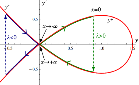
Figure 11: Graphical representation of the construction of solutions of the instanton equation for $\lambda>0$ (blue) and $\lambda<0$ (green). The dotted part of the curve represents the discontinuity in the derivative. The red line represents the $E=0$ solution of (80), the only one needed to solve the instanton equation with one local source.

This form does not make explicit that $\tilde{u}^{\lambda}(x)$ is analytic in $\lambda$ near $\lambda=0$. We will thus use the following equivalent form. Introduce $z=h_{\lambda}(x_{0})$. Equation (96) can then be rewritten as a cubic equation for $z\equiv z(\lambda)$,

$$\lambda=3z(1-z^{2})\ .$$ (97)

The trigonometric addition rules allow to rewrite

$$\begin{split}\tilde{u}^{\lambda}(x)&=\frac{3(1-z^{2})}{2\Big{[}\cosh\!\left(\frac{x}{2}\right)+z\sinh\!\left(\frac{|x|}{2}\right)\Big{]}^{2}}\\ &=\frac{6(1-z^{2})e^{-|x|}}{\big{[}1+z+(1-z)e^{-|x|}\big{]}^{2}}\ .\end{split}$$ (98)

The appropriate branch for (97) is the one for which $z\to 1$ as $\lambda\to 0$ (corresponding to $x_{0}\to\infty$). As can be seen in Fig. 12, this branch is defined for $\lambda\in]-\infty,\lambda_{c}=\frac{2}{\sqrt{3}}[$, while $z(\lambda)$ decreases from $z(-\infty)=\infty$ to $z_{c}=z(\lambda_{c})=1/\sqrt{3}$. The other branches are solutions of (93) but do not satisfy the physical requirements mentioned above.

Equations (97) and (98) thus define the solution to the instanton equation for $\lambda\in]-\infty,\lambda_{c}[$, in a way which is explicitly analytic around $\lambda=0$. For instance one can check that the small-$\lambda$ expansion

$$\tilde{u}^{\lambda}(x)=\frac{\lambda}{2}e^{-|x|}+\frac{\lambda^{2}}{6}\left(e^{-|x|}-\frac{1}{2}e^{-2|x|}\right)+\mathcal{O}(\lambda^{3})$$ (99)

obtained by iteratively solving Eq. (93) at small $\lambda$, is reproduced by Eqs. (97) and (98).

Finally the partition sum corresponding to an homogeneous kick is expressed as

$$Z(\lambda)=\int_{-\infty}^{\infty}\!\!\!dx~{}\tilde{u}^{\lambda}(x)=6(1-z)\ .$$ (100)

Hence, from Eq. (97), it satisfies

$$\lambda=\frac{1}{72}Z(Z-6)(Z-12)\ ,$$ (101)

recovering the result obtained in LeDoussalWiese2008c .

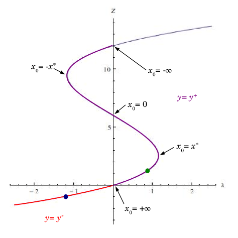
Figure 12: The generating function $Z(\lambda)=6(1-z)$ is represented here with some indications of the link with the construction of the instanton solution; the green and blue dot correspond to the solutions represented in figure 11.

B.2.2 Massless case

The massless instanton equation

$$\tilde{u}^{\prime\prime}(x)+\tilde{u}(x)^{2}=-\lambda\delta(x)$$ (102)

is solved similarly. For $\lambda<0$ there is a solution defined for all $x\in\mathbb{R}$,

$$\tilde{u}^{\lambda}(x)=-\frac{6}{(|x|+x_{0})^{2}}\quad,\quad x_{0}^{3}=-\frac{24}{\lambda}\ .$$ (103)

Note that for the massless case the physical solution is not required to be analytic in $\lambda$ at $\lambda=0$ (i.e. integer moments of avalanche sizes diverge). This solution can be obtained from (98) in the (formal) double limit of small $x$ and large $z$, with $x_{0}=2/z$. The equation determining $z$ now is $\lambda=-3z^{3}$. The generating function for a uniform kick becomes $Z=-6z=(72\lambda)^{1/3}$.

Appendix C Calculation of probabilities and densities of $S_{0}$

For an arbitrary kick $\delta w_{x}$, in the massive case, the Laplace transform of the distribution of local size is

$$\int\!\!dS_{0}\,e^{\lambda S_{0}}P_{\delta w_{x}}(S_{0})=\exp\!\left(\!L^{d-1}\int\!\!dx\,\delta w_{x}\tilde{u}^{\lambda}(x)\right)\ .$$ (104)

Here $\tilde{u}^{\lambda}(x)$ is given in Eq. (98). Performing the Laplace inversion in general is difficult, but there are some tractable cases.

C.1 Uniform kick

Let us start with a uniform kick $\delta w_{x}=\delta w$, and $\delta\hat{w}=L^{d}\delta w$. It is more efficient to take a a derivative of Eq. (104) w.r.t. $\lambda$ and write the Laplace inversion for $S_{0}P_{w}(S_{0})$,

$$S_{0}P_{\delta w}(S_{0})=\int_{C}\frac{d\lambda}{2i\pi}e^{-\lambda S_{0}}\partial_{\lambda}e^{6\delta\hat{w}(1-z(\lambda))}\ .$$ (105)

Here $C$ is an appropriate contour parallel to the imaginary axis and we used that $\int dx\,\tilde{u}(x)=6(1-z)$. The function $z(\lambda)$ is solution of $\lambda=3z(1-z^{2})$. One can now use $z$ as integration variable and rewrite

$$S_{0}P_{\delta w}(S_{0})=6\delta\hat{w}e^{6\delta\hat{w}}\int_{C}\frac{dz}{2i\pi}e^{-3z(1-z^{2})S_{0}}e^{-6\delta\hat{w}z}\ ,$$ (106)

using $d\lambda\partial_{\lambda}=dz\partial_{z}$. We will be sloppy here about the integration contour, as this procedure is heuristic to guess the result, which will then be tested (see below). As the exponential contains a cubic term, we use the Airy integral formula of Appendix A leading to

$$S_{0}P_{w}(S_{0})=6\delta\hat{w}e^{6\delta\hat{w}}\Phi(a,b,c)\ .$$ (107)

Here $\Phi$ is defined in Eq. (A), with $a=9S_{0}$, $b=0$ and $c=-(3S_{0}+6\delta\hat{w})$. This immediately leads to formula (21) in the main text. We have checked numerically that it reproduces the correct Laplace transform (104) for $\lambda<\lambda_{c}$.

C.2 Local kick

For a local kick it is possible to calculate the PDF of the local jump at the position of the kick.

Consider a local kick at $x=0$, i.e. $\delta w_{x}=\delta w_{0}\delta(x)$. For simplicity in this subsection we set $d=1$. Inserting this value in (104) we find that the LT of the PDF of the local size at the same point $S_{0}$ reads

$$\int dS_{0}\,e^{\lambda S_{0}}P_{\delta w_{0}}(S_{0})=e^{\frac{3}{2}(1-z^{2})\delta w_{0}}$$ (108)

using $\tilde{u}^{\lambda}(0)=\frac{3}{2}(1-z^{2})$. The same manipulations as above lead to

$$S_{0}P(S_{0}) = -\int_{C}\frac{dz}{2i\pi}e^{-3z(1-z^{2})S_{0}}\partial_{z}e^{\frac{3}{2}(1-z^{2})\delta w_{0}}$$

$$= 3\delta w_{0}e^{\frac{3\delta w_{0}}{2}}\int_{C}\frac{dz}{2i\pi}z~{}e^{-3z(1-z^{2})S_{0}-\frac{3}{2}z^{2}\delta w_{0}}$$

$$= 3\delta w_{0}e^{\frac{3\delta w_{0}}{2}}\partial_{c}\Phi(a,b,c)|_{a=9S_{0},b=-\frac{3\delta w_{0}}{2},c=-3S_{0}}\ .$$

Using Eq. (A) leads to

$$P_{\delta w_{0}}(S_{0}) = \frac{\delta w_{0}e^{\delta w_{0}-\frac{\delta w_{0}^{3}}{36S_{0}^{2}}}}{3^{1/3}S_{0}^{5/3}}\left[\frac{\delta w_{0}}{2\times 3^{1/3}S_{0}^{2/3}}\text{Ai}(u)-\text{Ai}^{\prime}(u)\right]$$

$$u = 3^{1/3}S_{0}^{2/3}+\frac{\delta w_{0}^{2}}{4\times 3^{2/3}S_{0}^{4/3}}\ .$$ (110)

We can check normalization, and that $\langle S_{0}\rangle=\frac{1}{2}\delta w_{0}$, consistent with the small-$\lambda$ expansion of (108). The asymptotics are

$$P_{\delta w_{0}}(S_{0})\simeq\left\{\begin{array}[]{ll}\dfrac{\delta w_{0}^{3/2}e^{\frac{\delta w_{0}}{2}-\frac{\delta w_{0}^{3}}{18S_{0}^{2}}}}{\sqrt{6\pi}S_{0}^{2}}&\text{for }\;S_{0}\ll 1\\ \vspace{-0.25cm}\\ \dfrac{\delta w_{0}e^{\delta w_{0}-\frac{2}{\sqrt{3}}S_{0}}}{2\sqrt[4]{3}\sqrt{\pi}S_{0}^{3/2}}&\text{for }\;S_{0}\gg 1\ .\end{array}\right.$$ (111)

This result, and the new exponent $\tau=5/3$ of the divergence at small $S_{0}$, which appear when $\delta w_{0}\to 0$, is discussed in the main text.

Appendix D Calculation of the joint density of $S$ and $S_{0}$

We will obtain the joint density from the generating function of $S_{0}$ and $S$,

$$\langle e^{\lambda S_{0}+\mu S}\rangle=e^{\int_{x}\delta w_{x}\tilde{u}_{x}}$$ (112)

in terms of the solution of the instanton equation. Let us consider a uniform kick $\delta w_{x}=\delta w$.

D.1 Instanton equation and its solution

D.1.1 Massive case

Here $\tilde{u}$ (that we will also denote $\tilde{u}^{\lambda,\mu}$ to make the dependence on the sources explicit) is the solution, in the variable $x$, of the instanton equation

$$\tilde{u}^{\prime\prime}-\tilde{u}+\tilde{u}^{2}=-\lambda\delta(x)-\mu\ .$$ (113)

We must solve this equation with similar requirements as discussed below for Eq. (93), except that now the instanton goes to a constant at infinity (since the source acts everywhere). Clearly, the new uniform source can be removed by a shift $\tilde{u}\rightarrow\tilde{u}+c$, where the constant $c$ verifies $\mu=c-c^{2}$. This results in the mass term $-\tilde{u}\to-(1-2c)\tilde{u}$, which can be brought back to Eq. (113) with $\mu=0$, i.e. Eq. (93), by a simple scale transformation. At the end one can check that given $\tilde{u}^{\lambda}(x)$ the solution of Eq. (93), the solution of Eq. (113), noted $\tilde{u}^{\lambda,\mu}(x)$, is given by

$$\tilde{u}^{\lambda,\mu}(x)=\frac{1-\beta^{2}}{2}+\beta^{2}\tilde{u}^{\lambda/\beta^{3}}(\beta x)\ .$$ (114)

The constant $\beta>0$ such that

$$\beta^{2}=\beta_{\mu}^{2}:=\sqrt{1-4\mu}\ .$$ (115)

In summary, the instanton solution is

$$\tilde{u}^{\lambda,\mu}(x)=\frac{1-\beta^{2}}{2}+\frac{6\beta^{2}(1-z^{2})e^{-\beta|x|}}{\big{[}1+z+(1-z)e^{-\beta|x|}\big{]}^{2}}\ ,$$ (116)

where $z$ is the solution of

$$\frac{\lambda}{\beta^{3}}=3z(1-z^{2})\ .$$ (117)

It is connected to $z=1$ at $\lambda=0$.

D.1.2 Massless case

It is useful to also give the solution in the massless case, for which one needs to solve

$$\tilde{u}^{\prime\prime}+\tilde{u}^{2}=-\lambda\delta(x)-\mu$$ (118)

for $\mu\leq 0$. Using a shift and a rescaling we can check that the solution now is

$$\tilde{u}^{\lambda,\mu}(x)=\frac{-\beta^{2}}{2}+\beta^{2}\tilde{u}^{\lambda/\beta^{3}}(\beta x)\ .$$ (119)

The parameter $\beta>0$ such that $\beta^{2}=\sqrt{-4\mu}$, and $\tilde{u}^{\lambda}(x)$ is the massive instanton solution. In summary, this gives

$$\tilde{u}^{\lambda,\mu}(x)=\frac{-\beta^{2}}{2}+\frac{6\beta^{2}(1-z^{2})e^{-\beta|x|}}{\big{[}1+z+(1-z)e^{-\beta|x|}\big{]}^{2}}$$ (120)

where $z$ is again the solution (117). If $\mu\to 0$, hence $\beta\to 0$ we recover the massless instanton (103).

D.2 Joint distribution

Let us again consider the massive case. To obtain the joint probability distribution $P_{\delta w}(S,S_{0})$, we need to calculate the generating function $Z(\lambda,\mu)$,

$$\begin{split}\langle e^{\lambda S_{0}+\mu S}\rangle=&\int_{0}^{\infty}\int_{0}^{\infty}P_{\delta w}(S_{0},S)e^{\lambda S_{0}+\mu S}dS\,dS_{0}\\ =&e^{\delta wZ\left(\lambda,\mu\right)}\end{split}$$ (121)

Integrating (116), we obtain

$$\begin{split}Z(\lambda,\mu)=\int_{x}\tilde{u}^{\lambda,\mu}(x)&=L^{d}\frac{1-\beta^{2}}{2}+L^{d-1}6\beta z(1-z)\\ &=:L^{d}Z_{1}(\mu)+L^{d-1}Z_{2}\left(\lambda,\mu\right)\ .\end{split}$$ (122)

$Z_{1}(\mu)$ is the generating function for the distribution of the total size of avalanches and $Z_{2}(\lambda,\mu)$ a new term defined by (122). The volume factors come from the coordinates along which the instanton solution is constant.

From equations (117) and (122), we can express $\lambda$ as a function of $Z_{2}$ and $\beta$,

$$\lambda=3\beta^{3}\left(1-{Z_{2}\over 6\beta}\right)\left[1-\left(1-{Z_{2}\over 6\beta}\right)^{2}\right]\ .$$ (123)

This is equivalent to $Z_{2}(\lambda,\mu)=\beta Z\left(\lambda\over\beta^{3}\right)$ where $Z\equiv Z(\lambda)$ is the generating function of the local size, which was implicitly defined as a solution of Eq. (101).

Considering the limit of small $\delta w$, we obtain $P_{\delta w}(S,S_{0})\approx\delta w\,\rho(S,S_{0})$, which defines the joint density $\rho(S,S_{0})$ of total and local sizes in the limit of a single avalanche. To simplify the computation, we decompose the distribution $\rho(S,S_{0})$ as

$$\rho(S,S_{0}) = \overline{\rho}(S,S_{0})+\delta(S_{0})\left(\rho(S)-\bar{\rho}(S)\right)$$

$$\bar{\rho}(S) = \int_{S_{0}>0}\overline{\rho}(S,S_{0})\ .$$ (124)

Here $\overline{\rho}(S,S_{0})$ is the smooth part of the joint density for $S$ and $S_{0}$, and is also the joint density of single avalanches containing $0$ (i.e. $S_{0}>0$). The second term takes into account all avalanches that occur away from $0$: the $\delta(S_{0})$ ensures that the avalanche does not contain $0$ and the subtraction ensure that $\int_{S_{0}}\rho(S,S_{0})=\rho(S)$ where $\rho(S)$ is the global size density. As we will check at the end of the calculation, the correct generating function for $\overline{\rho}$ is $Z_{2}(\lambda,\mu){L^{d-1}}+6\left(1-\beta_{\mu}\right){L^{d-1}}$.

As $\rho(S)$ is already known, we only want to compute $\overline{\rho}(S,S_{0})$. To eliminate the term $\delta(S_{0})$ we multiply (124) by $S_{0}$ and use that $S_{0}\rho(S,S_{0})=S_{0}\overline{\rho}(S,S_{0})$. Multiplication by $S_{0}$ is equivalent to taking a derivative w.r.t. $\lambda$ in the generating function,

$$\begin{split}S_{0}\,\overline{\rho}(S_{0},S)&=\,{L^{d-1}}\int_{-i\infty}^{i\infty}{d\mu\over 2\pi i}e^{-\mu S}\int_{-i\infty}^{i\infty}{d\lambda\over 2\pi i}e^{-\lambda S_{0}}\partial_{\lambda}Z_{2}\left(\lambda,\mu\right)\\ &=\,{L^{d-1}}\int_{-i\infty}^{i\infty}{d\mu\over 2\pi i}e^{-\mu S}\int_{-i\infty}^{i\infty}{dZ\over 2\pi i}e^{-{\beta^{3}\over 72}{Z\over\beta}\left(6-{Z\over\beta}\right)\left(12-{Z\over\beta}\right)S_{0}}\ .\end{split}$$ (125)

Here we changed variables from $\lambda$ to $Z_{2}$ (and dropped the indice) using (123). To simplify the calculations, we introduce a new variable $x$, s.t. $Z=2\times 3^{1\over 3}x+6\beta$, with $\beta$ defined in Eq. (115),

$$\begin{split}\overline{\rho}(S_{0},S)&={L^{d-1}}\times{2\times 3^{1\over 3}\over S_{0}}\,\int_{-i\infty}^{i\infty}{d\mu\over 2\pi i}e^{-\mu S}\int_{-i\infty}^{i\infty}{dx\over 2\pi i}e^{-{x^{3}\over 3}S_{0}+3^{1/3}\beta^{2}xS_{0}}\\ &={L^{d-1}}\times 2\times 3^{1\over 3}{e^{-S/4}\over S_{0}}\,\int_{-i\infty}^{i\infty}{dx\over 2\pi i}e^{-{x^{3}\over 3}S_{0}}{1\over 4}\int_{-i\infty}^{i\infty}{dy\over 2\pi i}e^{-{yS\over 4}+(-y)^{1/2}3^{1/3}xS_{0}}\\ &={L^{d-1}}\times 2\times 3^{1\over 3}{e^{-S/4}\over S_{0}}\,\int_{-i\infty}^{i\infty}{dx\over 2\pi i}e^{-{x^{3}\over 3}S_{0}}\int_{0}^{\infty}{dy\over 4\pi}e^{-{yS\over 4}}\sin\left(\sqrt{y}3^{1\over 3}xS_{0}\right)\\ &={L^{d-1}}\times 2\times 3^{2\over 3}{e^{-S/4}\over\sqrt{\pi}S^{3\over 2}S_{0}}\,\int_{-i\infty}^{i\infty}{dx\over 2\pi i}e^{-{x^{3}\over 3}S_{0}}xS_{0}e^{-{(3^{1/3}xS_{0})^{2}\over S}}\end{split}$$ (126)

The steps of this calculations are: first a linear change of variable $4\mu-1\rightarrow y$, such that $\beta=(-y)^{1\over 2}$, then a deformation of the contour of integration to integrate on both sides of the branch cut $\mathbb{R}^{+}$. Finally, the last integration can be performed in terms of Airy functions (e.g. using Appendix A),

$$\overline{\rho}(S,S_{0}) = \frac{6{L^{d-1}}}{\sqrt{\pi}S^{2}}e^{-{S\over 4}}F\!\left(\sqrt{3}S_{0}/S^{3\over 4}\right)$$ (127)

$$F(u) = {1\over u^{2\over 3}}e^{-{2\over 3}u^{4}}\left(u^{4\over 3}\text{Ai}\left(u^{8\over 3}\right)-\text{Ai}^{\prime}\left(u^{8\over 3}\right)\right)\ .$$

The density of avalanches with global size $S$ and which contain $0$, i.e. with $S_{0}>0$ is

$$\begin{split}\overline{\rho}(S)&=\int_{0}^{\infty}\!\!\!dS_{0}\,\overline{\rho}(S,S_{0})\\ &={L^{d-1}}\times 2\sqrt{{3\over\pi}}\bigg{[}\int_{0}^{\infty}\!\!du\,F(u)\bigg{]}{e^{-{S\over 4}}\over S^{5\over 4}}\\ &={L^{d-1}}{3\,\Gamma\left({1\over 4}\right)\over 2\pi}{e^{-{S\over 4}}\over S^{{5\over 4}}}\end{split}$$ (128)

where

$$\begin{split}{3\,\Gamma\left({1\over 4}\right)\over 2\pi}=2\sqrt{{3\over\pi}}\int_{0}^{\infty}duF(u)\approx 1.7311012158\ .\end{split}$$ (129)

To test our solution one can check that

$$\int_{0}^{\infty}\!\!\!ds{3\,\Gamma\left({1\over 4}\right)\over 2\pi}{e^{-{S\over 4}}\over S^{{5\over 4}}}(e^{\mu S}-1)=6\left[1-(1-4\mu)^{1\over 4}\right]\ .$$ (130)

We have checked numerically several other requirements, originating from the definitions, namely

$$\int_{0}^{\infty}\!\!\!dS\,\bar{\rho}(S,S_{0})=\rho_{0}(S_{0})=\frac{2{L^{d-1}}}{\pi S_{0}}K_{1/3}\!\left(2S_{0}/\sqrt{3}\right)$$

$$\int_{0}^{\infty}\!\!\!dS\int_{0}^{\infty}\!\!\!dS_{0}\,S_{0}\bar{\rho}(S,S_{0})={L^{d-1}}$$

$$\int_{0}^{\infty}\!\!\!dS\int_{0}^{\infty}\!\!\!dS_{0}\,S\bar{\rho}(S,S_{0})=6{L^{d-1}}$$

$$\int_{0}^{\infty}\!\!\!dS\int_{0}^{\infty}\!\!\!dS_{0}\,\bar{\rho}(S,S_{0})e^{\mu S}(e^{\lambda S_{0}}-1)=Z_{2}(\lambda,\mu){L^{d-1}}\ .$$

Appendix E Imposed local displacement

We set for simplicity $d=1$ in this section. The PDF of the global size in presence of imposed position driving is obtained from

$$\overline{e^{\mu S}}=e^{m^{2}\tilde{u}_{x=0}\delta w}\ ,$$ (131)

where $\tilde{u}_{x}$ is the solution of a slightly modified instanton equation:

$$\tilde{u}_{x}^{\prime\prime}-m^{2}\delta(x)\tilde{u}_{x}+\tilde{u}_{x}^{2}=-\mu$$ (132)

and we have kept explicit the local mass. This equation is the same as the massless Eq. (118), with $\lambda=-m^{2}\tilde{u}_{x=0}$, a self-consistency condition. Using its solution given in Eqs. (120) and (117) we eliminate $\lambda$ and $z$ in the system

$$\left\{\begin{array}[]{cl}\lambda&=-m^{2}\tilde{u}_{x=0}=-m^{2}\beta^{2}\left(1-\frac{3}{2}z^{2}\right)\\ \dfrac{\lambda}{\beta^{3}}&=3z(1-z^{2})\end{array}\right.$$ (133)

with $\beta=(-4\mu)^{1/4}$. It is then easy to see that there is a solution such that $m^{2}\tilde{u}_{x=0}$ remains finite when $m^{2}\to\infty$, in which case $z\to\sqrt{\frac{2}{3}}$ and

$$\lim_{m^{2}\to\infty}m^{2}\tilde{u}_{x=0}=-\sqrt{\frac{2}{3}}\beta^{3}\ .$$ (134)

Hence we find

$$P_{\delta w_{0}}(S)=\mbox{LT}^{-1}_{-\mu\to S}\,e^{-\delta w\sqrt{\frac{2}{3}}(-4\mu)^{3/4}}\ .$$ (135)

The result for the density is simpler,

$$S\rho(S)=-\mbox{LT}^{-1}_{-\mu\to S}\,\partial_{\mu}\sqrt{\frac{2}{3}}(-4\mu)^{3/4}\ ,$$ (136)

leading to

$$\rho(S)=\frac{\sqrt{3}}{\Gamma(1/4)S^{7/4}}$$ (137)

and a new exponent $7/4$ discussed in the main text.

Appendix F Some elliptic integrals for the extension distribution

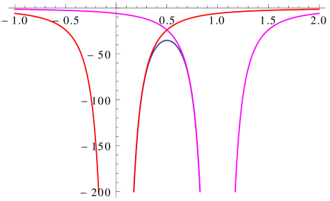
Figure 13: Instanton solutions involved in the computation of $Z(r)$ for $r=1$: in blue, $\tilde{u}_{1}(x)$, in red $\tilde{u}_{\infty}(x)$ and in purple, $\tilde{u}_{\infty}(x-1)$.

Here we make explicit the calculation for the density of extensions sketched in the main text. The relevant generating function, defined in the main text in Eq. (67), is

$$Z(r)=\int_{x}\tilde{u}_{r}(x)-\tilde{u}_{\infty}(x)-\tilde{u}_{\infty}(x-r)\ .$$ (138)

Here $\tilde{u}_{r}(x)$ is the solution of the instanton equation with two local sources, one at $x=0$ and one at $x=r$. The solution $\tilde{u}_{\infty}$ with one source at $x=0$ and one at infinity is equivalent to the solution with only one source at $x=0$.

The first simplification in the calculation of this integral is the symmetry arround $r/2$. Another is that, for $x\in]-\infty,0[$, $\tilde{u}_{r}(x)-\tilde{u}_{\infty}(x)$ cancels exactly. Then, the idea is to express the integral for $Z(r)$ without explicitly solving the instanton equation, using the change of variables

$$\int\tilde{u}\,dx=\int\tilde{u}\frac{du}{\tilde{u}^{\prime}}\ .$$ (139)

This requires to express the derivative of $\tilde{u}$ w.r.t. $x$ as a function of $\tilde{u}$, which is easy because $\tilde{u}$ is solution of a differential equation, and to decompose the integral into two parts such that the change of variables is well defined: from $x=-\infty$ to $x=0$ and from $x=0$ to $x=r/2$. The rest is deduced by symmetry.

In these two intervals, $\tilde{u}_{\infty}(x-r)$ does not contain a pole, and can safely be computed separately. Moreover, as we said, $\tilde{u}_{r}(x)-\tilde{u}_{\infty}(x)$ vanishes in the first interval, i.e. for $x\in]-\infty,0]$. This leaves only the integral of $\tilde{u}_{r}(x)-\tilde{u}_{\infty}(x)$ over $x$ running from $x=0$ to $x=r/2$. To simplify notations we introduce the variable $t<0$,

$$t:=\tilde{u}_{r}(r/2)\ ,$$ (140)

which is in one-to-one correspondance with $r$, and is a nice parameter to express $Z$. Indeed, after the change of variables (139), the integral now runs from $u=-\infty$ to $u=t$, and for $0<x<r/2$, with $\tilde{u}\equiv\tilde{u}_{r}$, we have

$$\tilde{u}_{r}^{\prime}=\sqrt{-t^{2}+\frac{2}{3}t^{3}+\tilde{u}^{2}-\frac{2}{3}\tilde{u}^{3}}\ .$$ (141)

Further, with $\tilde{u}\equiv\tilde{u}_{\infty}$,

$$\tilde{u}_{\infty}^{\prime}=\sqrt{\tilde{u}^{2}-\frac{2}{3}\tilde{u}^{3}}\ .$$ (142)

This comes from the results of Appendix B, and the relation $E=-t^{2}+\frac{2}{3}t^{3}$. To express $r$ in terms of $t$, we use the same idea as in the derivation of Eq. (139),

$$r=2\int_{0}^{r/2}dx=2\int_{-\infty}^{t}\frac{d\tilde{u}_{r}}{\tilde{u}_{r}^{\prime}}\ .$$ (143)

Putting these ingredients together, we obtain $Z(r)$ as a function of $t$, which we call $\tilde{Z}(t)$, in term of an elliptic integral, as well as the expression of $r$ as a function of $t$,

$$\begin{split}\tilde{Z}(t)&=2\int_{-\infty}^{t}\left({u\over\sqrt{-t^{2}+{2\over 3}t^{3}+u^{2}-{2\over 3}u^{3}}}-{u\over\sqrt{u^{2}-{2\over 3}u^{3}}}\right)du-2\int_{t}^{0}{u\over\sqrt{u^{2}-{2\over 3}u^{3}}}du\\ &=2t\int_{1}^{\infty}\left({y\over\sqrt{y^{2}-1-{2\over 3}t(y^{3}-1)}}-{1\over\sqrt{1-{2\over 3}ty}}\right)dy-6+2\sqrt{9-6t}\ ,\end{split}$$ (144)

$$r(t) = 2\int_{-\infty}^{t}{du\over\sqrt{-t^{2}+{2\over 3}t^{3}+u^{2}-{2\over 3}u^{3}}}$$ (145)

$$= 2\int_{1}^{\infty}{dy\over\sqrt{y^{2}-1-{2\over 3}t(y^{3}-1)}}\ .$$

We now use this to characterise the small-size divergence of the extension distribution. This is encoded in the small $r$ behavior of $Z(r)$, which corresponds to the large-$t$ behavior of $\tilde{Z}(t)$. For the latter, we have

$$\begin{split}Z(t)&\simeq-2\sqrt{3\over 2}\left[\int_{1}^{\infty}\!\!\!du\left({u\over\sqrt{u^{3}-1}}-{1\over\sqrt{u}}\right)-2\right]|t|^{1\over 2}\\ &\simeq 2\sqrt{6\pi}{\Gamma(5/6)\over\Gamma(1/3)}|t|^{1\over 2}\ ,\end{split}$$ (146)

which is also the exact result in the massless limit. We next need to invert Eq. (145) in the large-$t$ limit,

$$|t|\simeq A^{2}r^{-2}\;,\quad A=2\sqrt{6\pi}{\Gamma(7/6)\over\Gamma(2/3)}=\sqrt{6}\frac{\Gamma(1/3)^{3}}{4^{2/3}\pi}\ .$$ (147)

The small-$r$ behavior of $Z(r)$ is then given by

$$Z(r)\simeq 4\sqrt{3}\pi\,r^{-1}\ .$$ (148)

For small $|t|$ we find

$$r(t)\simeq 2\ln(12/|t|)$$ (149)

and

$$\tilde{Z}(t)\simeq t^{2}\ln(1/|t|)$$ (150)

which leads to

$$\tilde{Z}(r)=72~{}re^{-r}+O(e^{-r})$$ (151)

This leads to the tail of the extension density,

$$\rho(\ell)=\left.\partial_{r}^{2}\tilde{Z}(r)\right|_{r=\ell}\simeq 72\,\ell\,e^{-\ell}\text{ when }\ell\rightarrow\infty\ .$$ (152)

Appendix G Joint distribution for extension and total size

For simplicity, we consider only $m=0$ (massless limit). To obtain the joint distribution of extension and total size we have to add a global source $\mu$ to the instanton equation, in addition to the two local sources, whose parameters are sent to infinity. With the same tricks as previously, c.f. Appendix D and notably Eq. (119), we change this problem to a new one with a mass $\beta=(-4\mu)^{1\over 4}$, but no global source. The generating function is now a function of $r$, the distance between the two local sources and $\beta$, the new mass. As in Appendix F, we can change the variable $r$ to the new parameter $t$ defined in Eq. (140) and express everything in terms of elliptic integrals:

$$\begin{split}r(t,\beta)&=2\int_{t}^{\infty}{dy\over\sqrt{-\beta^{2}t^{2}-{2\over 3}t^{3}+\beta^{2}y^{2}+{2\over 3}y^{3}}}=\beta^{-1}f\left({t\over\beta^{2}}\right)\ ,\\ Z(t,\beta)&=-2\int_{t}^{\infty}\left({y\over\sqrt{-\beta^{2}t^{2}-{2\over 3}t^{3}+\beta^{2}y^{2}+{2\over 3}y^{3}}}-{1\over\sqrt{{2\over 3}y}}\right)+2\sqrt{6t}=\beta\,g\!\left({t\over\beta^{2}}\right)\ .\end{split}$$ (153)

The functions $f$ and $g$ are

$$\begin{split}f(x)&=2\int_{x}^{\infty}{du\over\sqrt{-x^{2}-{2\over 3}x^{3}+u^{2}+{2\over 3}u^{3}}}=2\int_{1}^{\infty}{du\over\sqrt{u^{2}-1+{2\over 3}x(u^{3}-1)}}\ ,\\ g(x)&=-2x\int_{1}^{\infty}\left({u\over\sqrt{u^{2}-1+{2\over 3}x(u^{3}-1)}}-{1\over\sqrt{{2\over 3}xu}}\right)+2\sqrt{6x}\ .\end{split}$$ (154)

From that, we have $Z(r,\beta)=\beta\left(g\circ f^{-1}\right)(\beta r)$ and then $\partial_{r}^{2}Z(r,\beta)=\beta^{3}\left(g\circ f^{-1}\right)^{\prime\prime}(\beta r)$ which gives

$$\rho(l,s)={1\over 4l^{7}}F\left({sl^{-4}\over 4}\right)\ ,$$ (155)

where $F$ is the inverse LT of $x\mapsto(-x)^{3\over 4}(g\circ f^{-1})^{\prime\prime}\left((-x)^{1\over 4}\right)$ with $g$ and $f$ the functions previously defined. Giving an analytic expression for this scaling function $F$ seems not to be possible.

Appendix H Numerics

We test most of our results with a direct numerical simulation of the equation of motion (1). This is done by discretizing both time and space. To avoid the $\sqrt{dt}$ term from a naive Euler time discretisation, we use the method of DornicChateMunoz2005 , which allows to express the exact propagator of the $d=0$ version of (1) in terms of random distributions (Poisson and Gamma distribution). We here review this result.

Let us start with the $d=0$ stochastic equation,

$$\partial_{t}\dot{u}_{t}=\alpha-\beta\dot{u}_{t}+\sqrt{2\sigma\dot{u}_{t}}\,\eta(t)$$ (156)

where $\eta$ is a Gaussian white noise and $\alpha$ is positive (so that $\dot{u}$ remains non-negative at all times). It can be integrated exactly using Bessel functions (cf. DobrinevskiLeDoussalWiese2011b for a derivation of this using the instanton equation for the ABBM model):

$$P(\dot{u}_{t}|\dot{u}_{0})=\frac{\beta}{\sigma}\frac{\sqrt{\frac{\dot{u}_{t}}{\dot{u}_{0}}}^{-1+\alpha}}{{2\sinh\left(\frac{\beta t}{2}\right)}}I_{-1+\alpha}\left(\frac{\beta}{\sigma}\frac{\sqrt{\dot{u}_{t}\dot{u}_{0}}}{\sinh\left(\frac{\beta t}{2}\right)}\right)\left(e^{\frac{\beta t}{2}}\right)^{\alpha}e^{-{\beta\over\sigma}\frac{\dot{u}_{0}e^{-\beta t}+\dot{u}_{t}}{1-e^{-\beta t}}}\ .$$ (157)

To use this representation efficiently in a numerical algorithm, the trick is to expand it in a series, and then express it as a combination of two distributions,

$$\begin{split}P(\dot{u}_{t}|\dot{u}_{0})=&\sum_{n=0}^{\infty}\frac{\dot{u}_{t}^{n-1+\alpha}\dot{u}_{0}^{n}}{n!\Gamma(n+\alpha)}\left(\frac{\beta}{2\sigma\sinh\left(\frac{\beta t}{2}\right)}\right)^{2n+\alpha}\left(e^{\frac{\beta t}{2}}\right)^{\alpha}e^{-\frac{\beta}{\sigma}\frac{\dot{u}_{0}}{e^{\beta t}-1}}e^{-\frac{\beta}{\sigma}\frac{\dot{u}_{t}}{1-e^{-\beta t}}}\\ =&\sum_{n=0}^{\infty}\text{Poisson}\left[\frac{\beta}{\sigma}\frac{\dot{u}_{0}}{e^{\beta t}-1}\right](n)\,\text{Gamma}\left[n+\alpha,\frac{1-e^{-\beta t}}{\beta}\sigma\right](\dot{u}_{t})\ .\end{split}$$ (158)

The Poisson and Gamma distributions used above are

$$\text{Poisson}\left[\lambda\right](n)=e^{-\lambda}\frac{\lambda^{n}}{n!}\,\text{for }n\in\mathbb{N}$$ (159)

$$\text{Gamma}\left[k,\theta\right](x)=\frac{1}{\theta(k-1)!}\left(\frac{x}{\theta}\right)^{k-1}e^{-\frac{x}{\theta}}\text{ for }x\in\mathbb{R}$$ (160)

This means that we can generate $\dot{u}_{t}$ at time $t$ from $\dot{u}_{0}$ by choosing first $n$ according to the Poisson distribution and then choosing $\dot{u}_{t}$ from a Gamma distribution with a shape depending on $n$. This can be summed up as a nice equality between random variables,

$$\dot{u}_{t}=\text{Gamma}\left[\text{Poisson}\left[\frac{\beta}{\sigma}\frac{\dot{u}_{0}}{e^{\beta t}-1}\right]+\alpha,\frac{1-e^{-\beta t}}{\beta}\sigma\right]~{}~{}~{}$$ (161)

To use this in a numerical simulation of Eq. (1), we first write a discretized (in space) version of the latter,

$$\partial_{t}\dot{u}_{i,t} = (\dot{u}_{i+1,t}+\dot{u}_{i-1,t})-(m^{2}+2)\dot{u}_{i,t}+\sqrt{2\sigma\dot{u}_{i,t}}\xi_{i,t}$$ (162)

$$+m^{2}\delta w_{i,t}\ .$$

Choosing $\alpha=\dot{u}_{i+1,t}+\dot{u}_{i-1,t}$, which is assumed to be constant on the time interval $[t,t+dt]$, and $\beta=m^{2}+2$ in Eq. (160) allows us to generate $\dot{u}_{i,t+dt}$, knowing all $\dot{u}_{i,t}$, with a correct probability distribution at order $dt$.

Appendix I Weierstrass and Elliptic functions

Here we recall some properties of Weierstrass’s elliptic function $\mathcal{P}$ (source AbramowitzStegun chapter 18, and Wolfram Mathworld). It appears in complex analysis as the only doubly periodic function on the complex plane with a double pole $1/z^{2}$ at zero. Denoting $\omega_{1},\omega_{2}$ the two (a priori complex) primitive half-periods, every point of the lattice $\Lambda=\{2m\omega_{1}+2n\omega_{2}|(n,m)\in\mathbb{Z}^{2}\}$ is a pole of order $2$ for $\mathcal{P}$. It can be constructed for $z\in\mathbb{C}-\Lambda$ as

$$\begin{split}&{\cal P}(z|\omega_{1},\omega_{2}):=\frac{1}{z^{2}}\\ &+\!\!\!\!\!\sum_{m,n\neq(0,0)}\frac{1}{(z-2m\omega_{1}-2n\omega_{2})^{2}}-\frac{1}{(2m\omega_{1}+2n\omega_{2})^{2}}\ .\end{split}$$ (163)

It is an even function of the complex variable $z$, with ${\cal P}(z)={\cal P}(-z)$. Note that the choice of primitive vectors $(2\omega_{1},2\omega_{2})$ is not unique, since one can alternatively choose any linear combination. The conventional choice of roots $g_{2}$ and $g_{3}$ is defined from its expansion around $z=0$,

$${\cal P}(z|\omega_{1},\omega_{2})=\frac{1}{z^{2}}+\frac{g_{2}}{20}z^{2}+\frac{g_{3}}{28}z^{4}+\mathcal{O}(z^{6})\ .$$ (164)

The function $\mathcal{P}$ is alternatively denoted

$${\cal P}(z|\omega_{1},\omega_{2})={\cal P}(z;g_{2},g_{3})$$ (165)

the latter being defined in Mathematica as $\text{WeierstrassP}[z,\{g_{2},g_{3}\}]$. More explicitly, the parameters $g_{2},g_{3}$ are expressed from the half-periods as

$$g_{2} = 60\!\!\!\!\!\sum_{m,n\neq(0,0)}\frac{1}{(2m\omega_{1}+2n\omega_{2})^{4}}\ ,$$ (166)

$$g_{3} = 140\!\!\!\!\!\sum_{m,n\neq(0,0)}\frac{1}{(2m\omega_{1}+2n\omega_{2})^{6}}\ .$$ (167)

The Weierstrass elliptic function verifies an interesting homogeneity property,

$$\mathcal{P}(\lambda z;\lambda^{-4}g_{2},\lambda^{-6}g_{3})=\lambda^{-2}\mathcal{P}(z;g_{2},g_{3})\ ,$$ (168)

and the non-linear differential equation

$${\cal P}^{\prime}(z)^{2}=4{\cal P}(z)^{3}-g_{2}{\cal P}(z)-g_{3}\ .$$ (169)

It is thus linked to elliptic integrals. Restricting now to $g_{2},g_{3}\in\mathbb{R}$ and focusing on $z\in\mathbb{R}$ one can choose one half-period to be real, which we denote $\Omega$ . The function ${\cal P}(z)$ is then periodic in $\mathbb{R}$ of period $2\Omega$ and diverges at all points $2m\Omega$, $m\in\mathbb{Z}$. It is defined in the fundamental interval $]0,2\Omega[$, repeated by periodicity. In this interval it satisfies the symmetry $\mathcal{P}(2\Omega-z;g_{2},g_{3})=\mathcal{P}(z;g_{2},g_{3})$. Its values in the first half-interval, i.e. for $z\in[0,\Omega]$ are such that (with $y\in[e_{1},\infty]$)

$$z=\int_{y}^{\infty}\frac{dt}{\sqrt{4t^{3}-g_{2}t-g_{3}}}\Leftrightarrow y=\mathcal{P}(z;g_{2},g_{3})$$ (170)

where $e_{1}$ is the largest real root of the polynomial in $t$

$$4t^{3}-g_{2}t-g_{3}=4(t-e_{1})(t-e_{2})(t-e_{3})\ .$$ (171)

The roots $e_{i}$ are all real if $\Delta=g_{2}^{3}-27g_{3}^{2}>0$ and only one, namely $e_{1}$, is real if $\Delta<0$. Hence the period is given by

$$\Omega=\int_{e_{1}}^{\infty}\!\!\!\frac{dt}{\sqrt{4t^{3}-g_{2}t-g_{3}}}\,,\;{\cal P}(\Omega)=e_{1}\,,\;{\cal P}^{\prime}(\Omega)=0\ .$$ (172)

It is always finite, except when $e_{1}$ is a double root, in which case $\Delta=0$ and the period is infinite $\Omega=\infty$.

For $g_{2}=0$ the integral (172) can be calculated explicitly using

$$\begin{split}\int_{1}^{\infty}\frac{du}{\sqrt{u^{3}-1}}&=\frac{\Gamma(1/3)^{3}}{4^{\frac{2}{3}}\pi}=\frac{-\sqrt{\pi}\,\Gamma(1/6)}{\Gamma(-1/3)}\ ,\\ \int_{-1}^{\infty}\frac{du}{\sqrt{u^{3}+1}}&=\sqrt{\pi}\frac{\Gamma(1/3)}{\Gamma(5/6)}\ .\end{split}$$ (173)

The half-periods are

$$\Omega=\left\{\begin{array}[]{ll}\dfrac{1}{4\pi}\Gamma(1/3)^{3}g_{3}^{-1/6}&\;\text{ when }\;g_{3}>0\\ \sqrt{\pi}\dfrac{\Gamma(1/3)}{4^{\frac{1}{3}}\Gamma(5/6)}|g_{3}|^{-1/6}&\;\text{ when }\;g_{3}<0\end{array}\right.\ ,$$ (174)

and the other period can be chosen as $\frac{1}{2}\Omega(1+i\sqrt{3})$.

Finally, taking another derivative of (169) we see that the Weierstrass function also satisfies

$${\cal P}^{\prime\prime}(z)=6{\cal P}(z)^{2}-\frac{g_{2}}{2}\ ,$$ (175)

and $\mathcal{P}(z;g_{2},g_{3})$ is the only solution of this differential equation which satisfies (164).

From this we can find solutions of the instanton equation

$$\tilde{u}_{x}^{\prime\prime}-A\tilde{u}_{x}+\tilde{u}_{x}^{2}=0\ ,$$ (176)

where $A=1$ is the massive case and $A=0$ the massless case. Comparing with Eq. (175) we see that a family of solutions are

$$\tilde{u}_{x}=\frac{A}{2}-6b^{2}{\cal P}\left(c+bx;\frac{A^{2}}{12b^{4}},g_{3}\right)\ .$$ (177)

Because of the homogeneity relation (168), this is a two-parameter family. These solutions are periodic. In the massless case $A=0$, the period of (177) is $\Omega/b$ where $\Omega$ is given by (174).

Appendix J Non-stationary dynamics

In the velocity theory the observables of the BFM are calculated from the dynamical action

$${\cal S}[\dot{u},\tilde{u}]=\int_{t,q}\tilde{u}_{-q,t}(\partial_{t}+q^{2}+m^{2})\tilde{u}_{q,t}-\sigma\int_{t,x}\tilde{u}_{xt}^{2}\dot{u}_{xt}$$

where $\tilde{u}$ is the response field. The quadratic part of the action, ${\cal S}_{0}$, defines the free response function,

$$\langle\dot{u}_{q,t}\tilde{u}_{q,t^{\prime}}\rangle_{{\cal S}_{0}}:=R_{q,t-t^{\prime}}=\theta(t-t^{\prime})e^{-(q^{2}+m^{2})(t-t^{\prime})}\ .$$ (178)

Standard perturbation theory in the disorder $\sigma$ is then performed, and has the peculiarity to contain only tree diagrams. It is easy to see that the average velocity is not corrected by the disorder, hence its value is the same as in the free theory. In presence of a uniform driving $w=vt$, and taking into account the initial condition $\dot{u}_{xt=0}=0$, one has

$$\overline{\dot{u}_{x,t}}=\langle\dot{u}_{xt}\rangle_{{\cal S}}=v\left(1-e^{-m^{2}t}\right)\ .$$ (179)

This implies

$$\overline{u_{xt}}=vt-\frac{1-e^{-m^{2}t}}{m^{2}}\ .$$ (180)

Next we compute the connected correlations, where $q$ means Fourier space and $x$ real space,

$$\overline{\dot{u}_{q,t_{1}}\dot{u}_{-q,t_{2}}}^{c} = \langle\dot{u}_{q,t_{1}}\dot{u}_{-q,t_{2}}\rangle_{{\cal S}}$$

$$= \sigma\int_{s,x}\langle\dot{u}_{q,t_{1}}\dot{u}_{-q,t_{2}}\tilde{u}_{x,s}^{2}\dot{u}_{x,s}\rangle_{{\cal S}_{0}}$$

$$= 2\sigma\int_{s}\langle\dot{u}_{xs}\rangle_{{\cal S}_{0}}R_{q,t_{1}-s}R_{q,t_{2}-s}\ .$$

Calculating this integral, and further integrating over $t_{1}$ and $t_{2}$ we obtain

$$\overline{u_{q,t}u_{-q,t}}^{c}=\int_{0}^{t}\!\!dt_{1}\int_{0}^{t}\!\!dt_{2}\;\overline{\dot{u}_{q,t_{1}}\dot{u}_{-q,t_{2}}}^{c}\ .$$ (182)

This is the final result given in the main text, see Eq. (74).

Alternatively we can obtain the correlations of $u_{xt}$ using

$$e^{\mu_{x}u_{xt_{1}}} =\int_{x}\mu_{x}\overline{U_{xt_{1}}}+\frac{1}{2}\int_{x_{1}x_{2}}\mu_{x_{1}}\mu_{x_{2}}\overline{U_{x_{1}t_{1}}U_{x_{2}t_{2}}}^{c}+...$$ (183)

$$=\exp\!\left(vm^{2}\int_{x,t>0}\tilde{u}^{\lambda}_{xt}\right)$$

where $\tilde{u}^{\lambda}_{xt}$ is the solution of the space-time dependent instanton equation with a source $\lambda_{xt}=\mu_{x}\theta(t)\theta(t_{1}-t)$. Using the perturbation method in the source of Section III.H of LeDoussalWiese2012a , specializing to that source in (261), we obtain at the end the same result as above.

References

- (1) S. Zapperi, P. Cizeau, G. Durin and H.E. Stanley, Dynamics of a ferromagnetic domain wall: Avalanches, depinning transition, and the Barkhausen effect, Phys. Rev. B 58 (1998) 6353–6366.
- (2) P. Le Doussal, K.J. Wiese, S. Moulinet and E. Rolley, Height fluctuations of a contact line: A direct measurement of the renormalized disorder correlator, EPL 87 (2009) 56001, arXiv:0904.1123.
- (3) D.S. Fisher, Collective transport in random media: From superconductors to earthquakes, Phys. Rep. 301 (1998) 113–150.
- (4) D. Bonamy, S. Santucci and L. Ponson, Crackling dynamics in material failure as the signature of a self-organized dynamic phase transition, Phys. Rev. Lett. 101 (2008) 045501.
- (5) S. Papanikolaou, F. Bohn, R.L. Sommer, G. Durin, S. Zapperi and J.P. Sethna, Universality beyond power laws and the average avalanche shape, Nature Physics 7 (2011) 316–320.
- (6) K. Dahmen and JP. Sethna, Hysteresis, avalanches, and disorder-induced critical scaling: A renormalization-group approach, Phys. Rev. B 53 (1996) 14872–14905.
- (7) T. Nattermann, S. Stepanow, L.-H. Tang and H. Leschhorn, Dynamics of interface depinning in a disordered medium, J. Phys. II (France) 2 (1992) 1483–8.
- (8) O. Narayan and D.S. Fisher, Threshold critical dynamics of driven interfaces in random media, Phys. Rev. B 48 (1993) 7030–42.
- (9) P. Le Doussal and K.J. Wiese, Size distributions of shocks and static avalanches from the functional renormalization group, Phys. Rev. E 79 (2009) 051106, arXiv:0812.1893.
- (10) P. Le Doussal and K.J. Wiese, First-principle derivation of static avalanche-size distribution, Phys. Rev. E 85 (2011) 061102, arXiv:1111.3172.
- (11) P. Le Doussal and K.J. Wiese, Distribution of velocities in an avalanche, EPL 97 (2012) 46004, arXiv:1104.2629.
- (12) A. Dobrinevski, P. Le Doussal and K.J. Wiese, Non-stationary dynamics of the Alessandro-Beatrice-Bertotti-Montorsi model, Phys. Rev. E 85 (2012) 031105, arXiv:1112.6307.
- (13) P. Le Doussal and K.J. Wiese, Avalanche dynamics of elastic interfaces, Phys. Rev. E 88 (2013) 022106, arXiv:1302.4316.
- (14) A. Dobrinevski, P. Le Doussal and K.J. Wiese, Avalanche shape and exponents beyond mean-field theory, EPL 108 (2014) 66002, arXiv:1407.7353.
- (15) B. Alessandro, C. Beatrice, G. Bertotti and A. Montorsi, Domain-wall dynamics and Barkhausen effect in metallic ferromagnetic materials. I. Theory, J. Appl. Phys. 68 (1990) 2901.
- (16) B. Alessandro, C. Beatrice, G. Bertotti and A. Montorsi, Domain-wall dynamics and Barkhausen effect in metallic ferromagnetic materials. II. Experiments, Journal of Applied Physics 68 (1990) 2908.
- (17) F. Colaiori, Exactly solvable model of avalanches dynamics for barkhausen crackling noise, Advances in Physics 57 (2008) 287, arXiv:0902.3173.
- (18) AA. Middleton, Asymptotic uniqueness of the sliding state for charge-density waves, Phys. Rev. Lett. 68 (1992) 670–673.
- (19) T. Thiery, P. Le Doussal and K.J. Wiese, Spatial shape of avalanches in the Brownian force model, J. Stat. Mech. 2015 (2015) P08019, arXiv:1504.05342.
- (20) A. Dobrinevski, Field theory of disordered systems – avalanches of an elastic interface in a random medium, arXiv:1312.7156 (2013).
- (21) A.I. Larkin, Sov. Phys. JETP 31 (1970) 784.
- (22) I. Dornic, H. Chaté and M.A. Muñoz, Integration of Langevin equations with multiplicative noise and the viability of field theories for absorbing phase transitions, Phys. Rev. Lett. 94 (2005) 100601.
- (23) M. Abramowitz and A. Stegun, Pocketbook of Mathematical Functions, Harri-Deutsch-Verlag, 1984.