Charmonia in a Contact Interaction

Abstract

For the flavour-singlet heavy quark system of charmonia, we compute the masses of the ground state mesons in four different channels: pseudo-scalar ($\eta_{c}(1S)$), vector ($J/\Psi(1S)$), scalar ($\chi_{c_{0}}(1P)$) and axial vector ($\chi_{c_{1}}(1P)$), as well as the weak decay constants of the $\eta_{c}(1S)$ and $J/\Psi(1S)$ and the charge radius of $\eta_{c}(1S)$. The framework for this analysis is provided by a symmetry-preserving Schwinger-Dyson equation (SDEs) treatment of a vector$\times$vector contact interaction (CI). The results found for the meson masses and the weak decay constants, for the spin-spin combinations studied, are in fairly good agreement with experimental data and earlier model calculations based upon Schwinger-Dyson and Bethe-Salpeter equations (BSEs) involving sophisticated interaction kernels. The charge radius of $\eta_{c}(1S)$ is consistent with the results from refined SDE studies and lattice Quantum Chromodynamics (QCD).

I Introduction

Quantum Chromodynamics (QCD) and the resulting hadron bound states form a challenging sector of the Standard Model of particle physics. In the non perturbative regime of these interactions, the emergent phenomena of chiral symmetry breaking and confinement govern their spectrum and properties. Within the framework of Schwinger-Dyson equations (SDEs), we can study the structure of strongly interacting bound states through first principles in the continuum. SDEs for QCD have been extensively applied to the study of light quark Jain and Munczek (1993); Maris et al. (1998); Maris and Tandy (1999) and gluon propagators Boucaud et al. (2008); Aguilar et al. (2008); Pennington and Wilson (2011), their interactions Chang and Roberts (2009); Kizilersu and Pennington (2009); Bashir et al. (2012a), meson spectra below the masses of 1 GeV as well as their static and dynamic properties.

First explorations for heavy mesons, both charmonia and bottomonia, with a consistent use of the rainbow-ladder truncation in the kernels of the gap and Bethe-Salpeter equations (BSEs), were undertaken by Jain and Munczek in Ref. Jain and Munczek (1993). They found the mass spectrum and the decay constants of pseudoscalar mesons in good agreement with experiments. This work was repeated with the Maris-Tandy model for $\bar{c}c$ bound states in Refs. Krassnigg and Maris (2005); Bhagwat et al. (2007) with extrapolations to the $\bar{b}b$ systems in Refs. Maris and Tandy (2006); Blank and Krassnigg (2011). A full numerical solution for flavour-singlet pseudoscalar mesons again yielded charmonia and bottomonia masses and decay constants consistent with experimental data; predictions for states with exotic quantum numbers were also made in Refs. Maris (2007); Krassnigg (2009). The effect of the quark-gluon interaction in the gap equation and the vertex-consistent Bethe-Salpeter kernel was investigated in Ref. Bhagwat et al. (2004). More recently, employing a parametrization of the quark propagator to analytically continue it into the complex plane, heavy quark systems were studied in detail in Ref. Souchlas (2010). A more direct approach through the numerical computation of the quark propagator in the required region of the complex plane was employed in Ref. Rojas et al. (2014). There the mass spectrum and decay constants for flavor singlet $J^{P}=0^{-}$ mesons were reported.

The extension of this program to the complicated exotic and baryonic states, decay rates and form factors is, numerically, not straightforward at all. A few years ago, an alternative was explored to initially study pion properties assuming that quarks interact not via massless vector-boson exchange but instead through a symmetry preserving vector-vector contact interaction (CI) Gutierrez-Guerrero et al. (2010); Roberts et al. (2010); Chen et al. (2012); Roberts et al. (2011a, b). One then proceeds by embedding this interaction in a rainbow-ladder truncation of the SDEs. Confinement is implemented by employing a proper time regularization scheme. This scheme systematically removes quadratic and logarithmic divergences ensuring that the axial-vector Ward-Takahashi identity (axWTI) is satisfied. One can also explicitly verify the low energy Goldberger-Treiman relations. A fully consistent treatment of the CI model is simple to implement and can help us provide useful results which can be compared and contrasted with full QCD calculation and experiment.

This interaction is capable of providing a good description of the masses of meson and baryon ground and excited-states for light quarks Gutierrez-Guerrero et al. (2010); Roberts et al. (2010); Chen et al. (2012); Roberts et al. (2011a). The results obtained from the CI model are quantitatively comparable to those obtained using sophisticated QCD model interactions, Bashir et al. (2012b); Eichmann et al. (2008); Maris (2007); Cloet et al. (2007). Interestingly and importantly, this simple CI produces a parity-partner for each ground-state that is always more massive than its first radial excitation so that, in the nucleon channel, e.g., the first $J^{P}={1}/{2}^{-}$ state lies above the second $J^{P}={1}/{2}^{+}$ state  Chen et al. (2012).

We take this as a sufficient justification to employ this interaction for the analysis of the quark model heavy mesons for spins $J=0,1$ and study the mass spectrum and weak decay constants for charmonia. Without parameter readjustment, we find good agreement with charmonia masses. However, we need to modify the set of parameters to simultaneously account for the weak decay constants of the $\eta_{c}(1S)$ and $J/\Psi(1S)$, and the charge radius of $\eta_{c}(1S)$.

The paper is organized as follows: in Section II we present the necessary details of the SDE-BSE approach to mesons; while in Section III and Section IV we introduce the interaction used and the consequences of the axWTI;  Section V outlines the general forms of the Bethe-Salpeter amplitude (BSA) for the mesons studied; Section VI contains numerical analysis of the results obtained without readjusting the parameters of the light quark sector; while in  Section VII we minimally modify the CI model parameters and re-evaluate the charmonia masses, decay constants of $\eta_{c}(1S)$ and $J/\Psi(1S)$, and the charge radius of $\eta_{c}(1S)$; finally in Section VIII, we state our findings and present our conclusions and discussion.

II The Bethe-Salpeter and the Gap Equations

Meson bound states appear as poles in a four-point function. The condition for the appearance of these poles in a particular $J^{PC}$ channel is given by the homogeneous BSE Gross (1993); Salpeter and Bethe (1951); Gell-Mann and Low (1951)

$$\left[\Gamma_{H}(k;P)\right]_{tu}=\int\frac{\mathrm{d}^{4}q}{(2\pi)^{4}}\,\chi(q;P)_{sr}K^{rs}_{tu}(q,k;P)\,,$$ (1)

where $\chi(q;P)=S_{f}(q_{+})\Gamma_{H}(q;P)S_{g}(q_{-})$; $q_{+}=q+\eta P$, $q_{-}=q-(1-\eta)P$; $k$ ($P$) is the relative (total) momentum of the quark-antiquark system; $S_{f}$ is the $f$-flavour quark propagator; $\Gamma_{H}(q;P)$ is the meson BSA, where $H=f\overline{g}$ specifies the flavour content of the meson; $r,s,t,u$ represent colour, flavour, and spinor indices; and $K$ is the quark-antiquark scattering kernel. For a comprehensive recent review of the BSE and its applications, see Bashir et al. (2012b).

The $f$-flavour dressed-quark propagator, $S_{f}$, that enters Eq. (1) is obtained as the solution of the quark SDE, the so called gap equation Roberts et al. (2007); Holl et al. (2006); Maris and Roberts (2003); Alkofer and von Smekal (2001):

$$S_{f}^{-1}(p)=i\gamma\cdot p+m_{f}+\Sigma_{f}(p)\,,$$ (2)

$$\Sigma_{f}(p)=\int\frac{\mathrm{d}^{4}q}{(2\pi)^{4}}\,g^{2}D_{\mu\nu}(p-q)\frac{\lambda^{a}}{2}\gamma_{\mu}S_{f}(q)\Gamma^{a}_{\nu}(p,q)\,,$$ (3)

where $g$ is the strong coupling constant, $D_{\mu\nu}$ is the dressed-gluon propagator, $\Gamma^{a}_{\nu}$ is the dressed-quark-gluon vertex, and $m_{f}$ is the bare $f$-flavour current-quark mass. Since the CI, to be defined later in Section III, is non-renormalizable, it is not necessary to introduce any renormalziation constant, and the chiral limit is obtained by setting $m_{f}=0$ Roberts et al. (2007); Holl et al. (2006); Maris and Roberts (2003).

Both $D_{\mu\nu}$ and $\Gamma^{a}_{\nu}$ satisfy their own SDE, which in turn are coupled to higher $n$-point functions and so on ad infinitum. Therefore, the quark SDE, Eq. (2), is only one of the infinite set of coupled nonlinear integral equations. A tractable problem is defined once a truncation scheme has been specified, i.e., once the gluon propagator and the quark-gluon vertex are defined.

III Rainbow-Ladder truncation and the Contact Interaction

$m$	$M$	$E_{\pi}$	$F_{\pi}$	$E_{\rho}$	$m_{\pi}$	$m_{\rho}$	$f_{\pi}$	$f_{\rho}$
0	0.358	3.568	0.459	1.520	0	0.919	0.100	0.130
0.007	0.368	3.639	0.481	1.531	0.140	0.928	0.101	0.129

Table 1: Results for light pseudoscalar and vector mesons obtained with $m_{g}=0.8\,\text{GeV}$, $\alpha_{IR}=0.93\pi$, $\Lambda_{\text{IR}}=0.24\,\text{GeV}$, $\Lambda_{\text{UV}}=0.905\,\text{GeV}$. These model parameters were determined in Refs. Roberts et al. (2011a); Chen et al. (2012)

It has been shown  Gutierrez-Guerrero et al. (2010); Roberts et al. (2010); Chen et al. (2012); Roberts et al. (2011a) that a momentum-independent vector$\times$vector CI is capable of providing a description of light pseudoscalar and vector mesons static properties, which is comparable to that obtained using more sophisticated QCD model interactions Bashir et al. (2012b); Eichmann et al. (2008); Maris (2007); Cloet et al. (2007); see for example Table 1. We employ this interaction for the analysis of the quark model charmonia spectrum. We therefore use

$$g^{2}D_{\mu\nu}(k)=\frac{4\pi\alpha_{\rm IR}}{m_{g}^{2}}\delta_{\mu\nu}\equiv\frac{1}{m_{G}^{2}}\delta_{\mu\nu}\,,$$ (4)

in Eq. (3), where $m_{g}=800$ MeV is a gluon mass scale which is in fact generated dynamically in QCD, see for example Boucaud et al. (2012), and $\alpha_{\rm IR}=0.93\pi$ is a parameter that determines the interaction strength. For the quark-gluon vertex, the rainbow truncation will be used:

$$\Gamma^{a}_{\mu}(p,q)=\frac{\lambda^{a}}{2}\gamma_{\mu}\,.$$ (5)

Once the elements of the kernel in the quark SDE have been specified, we can proceed to obtain and analyse its solution. The general form of the f-flavoured dressed quark propagator, obtained as the solution of Eq. (2), is given in terms of two Lorentz-scalar dressing functions, written in two different but equivalent forms as:

$$S^{-1}_{f}(p) = \mathrm{i}\gamma\cdot pA_{f}(p^{2})+B_{f}(p^{2})$$ (6)

$$= Z^{-1}_{f}(p^{2})\left(i\gamma\cdot p+M_{f}(p^{2})\right)\,.$$ (7)

In the latter expression, $Z(p^{2})$ is known as the wave-function renormalization, and $M_{f}(p^{2})$ is the dressed, momentum-dependent quark mass function, which connects current and constituent quark masses Roberts et al. (2007); Holl et al. (2006); Maris and Roberts (2003).

Using Eq. (4) and Eq. (5), the quark equation, Eq. (2), takes the following simple form

$$S^{-1}_{f}(p)=i\gamma\cdot p+m_{f}+\frac{4}{3}\frac{1}{m_{G}^{2}}\int\frac{\mathrm{d}^{4}q}{(2\pi)^{4}}\,\gamma_{\mu}S_{f}(q)\gamma_{\mu}\,.$$ (8)

The solution to this equation is of the form

$$S_{f}^{-1}(p)=\mathrm{i}\gamma\cdot p+M_{f}\,,$$ (9)

since the last term on the right-hand side of Eq. (8) is independent of the external momentum. The momentum-independent mass, $M_{f}$, is determined as the solution of

$$M_{f}=m_{f}+\frac{M_{f}}{3\pi^{2}m_{G}^{2}}\int_{0}^{\infty}\mathrm{d}s\,s\frac{1}{s+M_{f}^{2}}\,.$$ (10)

Since Eq. (10) is divergent, we have to specify a regularization procedure. We employ the proper time regularization scheme, Ebert et al. (1996), and write:

$$\frac{1}{s+M^{2}} = \int_{0}^{\infty}\mathrm{d}\tau\,\mathrm{e}^{-\tau(s+M^{2})}\to\int_{\tau_{\rm{UV}}^{2}}^{\tau_{{\rm{IR}}^{2}}}\mathrm{d}\tau\,\mathrm{e}^{-\tau(s+M^{2})},$$ (11)

$$= \frac{\mathrm{e}^{-\tau_{\text{U}V}^{2}(s+M^{2})}-\mathrm{e}^{-\tau_{\text{I}R}^{2}(s+M^{2})}}{s+M^{2}}\,,$$

where $\tau_{\text{IR}}^{2}$ and $\tau_{\text{UV}}^{2}$ are, respectively, infrared and ultraviolet regulators. A nonzero value for $\tau_{\text{IR}}\equiv 1/\Lambda_{\text{IR}}$ implements confinement by ensuring the absence of quark production thresholds  Roberts (2008). Furthermore, since Eq. (4) does not define a renormalizable theory, $\tau_{\text{UV}}\equiv 1/\Lambda_{\text{UV}}$ cannot be removed, but instead plays a dynamical role and sets the scale for all dimensioned quantities. Note that the role of ultraviolet cut-off in Nambu–Jona-Lasinio type models has also been discussed in Refs. Farias et al. (2006, 2008). Thus

$$M_{f}=m_{f}+\frac{M_{f}}{3\pi^{2}m_{G}^{2}}\mathcal{C}_{01}(M_{f}^{2};\tau_{\text{IR}},\tau_{\text{UV}})\,,$$ (12)

where

$$\mathcal{C}_{\alpha\beta}(M^{2};\tau_{\text{IR}},\tau_{\text{UV}})=\frac{\left(M^{2}\right)^{\nu}}{\Gamma(\beta)}\Gamma(\beta-2,\tau_{\text{UV}}^{2}M^{2},\tau_{\text{IR}}^{2}M^{2})\,,$$ (13)

with $\nu=\alpha-(\beta-2)$ and $\Gamma(a,z_{1},z_{2})$ is the generalized incomplete gamma function.

IV Axial-Vector Ward-Takahashi Identtiy

The phenomenological features of chiral symmetry and its dynamical breaking in QCD can be understood by means of the axWTI. In the chiral limit, it reads

$$-\mathrm{i}P_{\mu}\Gamma_{5\mu}(k;P)=S^{-1}(k_{+})\gamma_{5}+\gamma_{5}S^{-1}(k_{-})\,.$$ (14)

The axWTI relates the axial-vector vertex, $\Gamma_{5\mu}$, the pseudoscalar vertex, $\gamma_{5}$ and the quark propagator. This in turn implies a relationship between the kernel in the BSE and that in the quark SDE. It must be preserved by any viable truncation scheme of the SDE-BSE coupled system. It is the preservation of this identity which proves useful in obtaining the defining characteristics of the octet of pseudoscalar mesons, namely their low mass, their masslessness in the chiral limit, and the hadron mass splittings Maris et al. (1998); Weise (2005)

The axial-vector vertex satisfies its own SDE, namely

$$\Gamma_{5\mu}(k;P)=\gamma_{5}\gamma_{\mu}+\int\frac{\mathrm{d}^{4}q}{(2\pi)^{4}}\,K(k,q;P)\chi_{5\mu}(q;P)\,,$$ (15)

where the appropriate indices are contracted and $K(k,q;P)$ is the Bethe-Salpeter kernel that appears in the bound state Eq. (1). A similar equation is satisfied by the pseudoscalar vertex.

Combining the SDEs satisfied by the pseudovector and pseudoscalar vertices with the axWTI one arrives at Maris et al. (1998)

$$\int\frac{\mathrm{d}^{4}q}{(2\pi)^{4}}\,K_{tu;rs}(k,q;P)\left[\gamma_{5}S(q_{-})+S(q_{+})\gamma_{5}\right]_{sr}\\ =\left[\Sigma(k_{+})\gamma_{5}+\gamma_{5}\Sigma(k_{-})\right]_{tu}\,,$$ (16)

thus constraining the content of the quark-antiquark scattering kernel $K(p,q;P)$ if an essential symmetry of the strong interactions, and its breaking pattern, is to be faithfully reproduced.

From a practical point of view, Eq. (16) provides a way of obtaining the quark-antiquark scattering kernel if we can solve this constraint, given an expression for the quark self-energy. However, this is not always possible, see e.g. Fischer et al. (2007), and we must find an alternative way of preserving the chiral symmetry properties of the strong interactions. In principle, one may construct a quark-antiquark scattering kernel satisfying Eq. (16) from a functional derivative of the quark self-energy with respect to the quark propagator Munczek (1995), within the framework of the effective action formalism for composite operators developed in Cornwall et al. (1974).

Fortunately, for the CI model under study, Eq. (16) can be easily satisfied. The resulting expression for the scattering kernel is called the rainbow-ladder (RL) truncation. This kernel is the leading-order term in a non perturbative, symmetry-preserving truncation scheme, which is known and understood to be accurate for pseudoscalar and vector mesons. Moreover, it guarantees electromagnetic current conservation Roberts (2008):

$$K(p,q;P)_{tu;rs}=-\frac{1}{m_{G}^{2}}\delta_{\mu\nu}\left[\frac{\lambda^{a}}{2}\gamma_{\mu}\right]_{ts}\left[\frac{\lambda^{a}}{2}\gamma_{\nu}\right]_{ru}\,.$$ (17)

Using the interaction we have specified, Eqs. (4,5), the homogeneous BSE for a meson ($\eta=1$) takes a simpler form,

$$\Gamma_{H}(k;P)=-\frac{4}{3}\frac{1}{m_{G}^{2}}\int\frac{\mathrm{d}^{4}q}{(2\pi)^{4}}\,\gamma_{\mu}S_{f}(q+P)\Gamma_{H}(q;P)S_{g}(q)\gamma_{\mu}\,.$$ (18)

Since the interaction does not depend on the relative momentum of the quarks, a symmetry-preserving regularization of Eq. (18) will yield solutions which are independent of it. It follows that if the interaction of Eq. (4) produces bound states, then the relative momentum between the quark and the antiquark can assume any value with equal probability. This is the defining characteristic of a point-like particle.

IV.1 A Corollary of the Axial-Vector WTI

There are further non trivial consequences of the axWTI and the CI. They define our regularization procedure, which must maintain

$$0=\int\frac{\mathrm{d}^{4}q}{(2\pi)^{4}}\,\left[\frac{P\cdot q_{+}}{q_{+}^{2}+M_{f}^{2}}-\frac{P\cdot q}{q_{-}^{2}+M_{g}^{2}}\right]\,.$$ (19)

This ensures that Eq. (14) is satisfied. Now analyzing the integrands, using a Feynman parametrization, one arrives at the following identity for $P^{2}=0=m$, and $M_{f}=M_{g}=M$:

$$0=\int\frac{\mathrm{d}^{4}q}{(2\pi)^{4}}\,\frac{\frac{1}{2}q^{2}+M^{2}}{\left(q^{2}+M^{2}\right)^{2}}\,.$$ (20)

Eq. (20) states that the axWTI is satisfied if, and only if, the model is regularized so as to ensure there are no quadratic or logarithmic divergences. Unsurprisingly, these are the circumstances under which a shift in integration variables is permitted, an operation required in order to prove Eq. (14).

It is notable that Eq. (14) is also valid for arbitrary $P$. Using a Feynman parametrization of the integrand, and making an appropriate change of variables ($q\to q-xP$) to diagonalize the denominator, we find, for non zero $P^{2}$

$$0=\int_{0}^{1}\mathrm{d}x\,\int\frac{\mathrm{d}^{4}q}{(2\pi)^{4}}\,\frac{\frac{1}{2}q^{2}+\mathfrak{M}^{2}}{\left(q^{2}+\mathfrak{M}^{2}\right)^{2}}\,,$$ (21)

where $\mathfrak{M}^{2}=M_{f}^{2}x+M_{g}^{2}(1-x)+x(1-x)P^{2}$. This constraint will be implemented in all our calculations so that Eq. (14) is preserved.

V Classification of BSA in a Contact Interaction

We are interested in the static properties of several mesons. We thus begin with their classification and the general form of their BSA in the CI we are working with. Table 2 lists the spin quantum numbers of the quark model mesons we will study.

$L$	$J^{PC}$	Type	$L$	$J^{PC}$	Type
$0$	$0^{-+}$	Pseudoscalars	$1$	$0^{++}$	Scalars
$0$	$1^{--}$	Vectors	$1$	$1^{++},\,1^{+-}$	Axial Vectors

Table 2: Quark model mesons

With the dependence on the relative momentum forbidden by the CI, the general form of the BSAs for the mesons listed in Table 2 are  Llewellyn-Smith (1969):

$$\Gamma_{0^{-+}}(P) = \gamma_{5}\left[\mathrm{i}E_{0^{-+}}+\frac{1}{2M}\gamma\cdot PF_{0^{-+}}\right]\,,$$ (22)

$$\Gamma_{0^{++}}(P) = \mathbb{1}E_{0^{++}}\,,$$ (23)

$$\Gamma_{1^{--}\mu}(P) = \gamma^{T}_{\mu}E_{1^{--}}+\frac{1}{2M}\sigma_{\mu\nu}P_{\nu}F_{1^{--}}\,,$$ (24)

$$\Gamma_{1^{++}\mu}(P) = \gamma_{5}\left[\gamma^{T}_{\mu}E_{1^{++}}+\frac{1}{2M}\sigma_{\mu\nu}P_{\nu}F_{1^{++}}\right]\,,$$ (25)

where $M$ is a mass scale, to be defined later. Results will be independent of its choice. A charge-conjugated BSA is obtained, in general, via

$$\overline{\Gamma}_{H}(k;P)=C^{\dagger}\Gamma(-k;P)^{T}C,$$ (26)

where $T$ denotes the transposing of all matrix indices and $C=\gamma_{2}\gamma_{4}$ is the charge conjugation matrix, with $C^{\dagger}=-C$, and $[C,\gamma_{5}]=0$. We thus have

$$C^{\dagger}\gamma_{\mu}^{T}C = -\gamma_{\mu}\,,$$ (27)

$$C^{\dagger}\sigma_{\mu\nu}^{T}C = -\sigma_{\mu\nu}\,,$$ (28)

$$C^{\dagger}\gamma_{5}^{T}C = \gamma_{5}\,,$$ (29)

$$C^{\dagger}\gamma_{5}\sigma^{T}_{\mu\nu}C = -\gamma_{5}\sigma_{\mu\nu}\,,$$ (30)

$$C^{\dagger}(\gamma_{5}\sigma_{\mu\nu})^{T}C = \gamma_{5}\gamma_{\mu}\,,$$ (31)

and therefore

$$\overline{\Gamma}^{0^{++}}(P) = \Gamma^{0^{++}}(P),$$ (32)

$$\overline{\Gamma}^{1^{--}}_{\mu}(P) = -\Gamma^{1^{--}}_{\mu}(P),$$ (33)

$$\overline{\Gamma}^{1^{++}}_{\mu}(P) = \Gamma^{1^{++}}_{\mu}(P).$$ (34)

It is a well known feature of the rainbow-ladder truncation of the SDE-BSE system that it describes the pseudoscalar and vector mesons well, but not their parity partners, namely, the scalar and axial-vector mesons. In more realistic kernels, see for example Chang and Roberts (2009), when the quark-gluon vertex is fully dressed, it was found that dynamical chiral symmetry breaking (DCSB) generates a large dressed-quark anomalous chromo-magnetic moment in the infrared. Consequently, the associated corrections cancel in the pseudoscalar and vector channels but add in the scalar and axial vector channels, resulting in a magnified splitting between parity partners. This effect is specially important for mesons made up of light quarks. With this in mind, following Ref. Roberts et al. (2011a), we have introduced a spin-orbit repulsion into the scalar- and axial-vector-meson channels through the artifice of a phenomenological coupling $g_{SO}^{2}\leq 1$, introduced as a factor multiplying the scalar and axial-vector kernels. The value $g_{SO}=0.24$ was chosen in Ref. Roberts et al. (2011a) so as to obtain the experimental value for the $a_{1}$-$\rho$ mass splitting which is known to be achieved by the corrections described above (without the spin-orbit coupling $g_{SO}$, the mass difference between the $a_{1}$ and the $\rho$ is 0.15 GeV, a factor of 3 smaller than the experimental value, It implies that the spin-orbit coupling has increased the mass of the $a_{1}$ by $28\%$, which is a large effect).

VI Numerical Results

The mass and BSA of a meson depend on its quantum numbers and can be found by solving Eq. (1). In order to do this, we will introduce a fictitious eigenvalue $\lambda_{H}$ to the bound state equation. Thus, the mass of the bound state in a particular channel, $m_{H}$, will be such that $\lambda_{H}(P^{2}=-m_{H}^{2})=1$, where $P$ is the meson’s momentum. In any channel, the form of the homogeneous BSE for the CI will be

$$K_{H}(m_{H})\cdot\Gamma_{H}(m_{H})=\lambda_{H}(m_{H})\Gamma_{H}(m_{H})\,,$$ (35)

where $K_{H}$ is a $2\times 2$ matrix, and the subscript $H$ indicates the dependence of the explicit expressions on the quantum numbers of the meson under consideration, see Eqs. (22-25). Equation (35) is an eigenvalue equation for the vector $\Gamma_{H}(m_{H})=(E_{H}(m_{H}),F_{H}(m_{H}))^{T}$ with solutions for discrete values of $P^{2}=-m_{H}^{2}$. Explicit expressions for every channel given in Table 2 are presented in Appendix A.

	masses
	$m_{\eta_{c}(1S)}$	$m_{J/\Psi(1S)}$	$m_{\chi_{c_{0}}(1P)}$	$m_{\chi_{c_{1}}(1P)}$
Experiment  Nakamura and Group (2010)	2.983	3.096	3.414	3.510
Contact Interaction	2.983∗	2.979	3.412	3.442
	-	-	3.293	3.344
JM Jain and Munczek (1993)	2.821	3.1	3.605	-
BK Blank and Krassnigg (2011)	2.928	3.111	3.321	3.437
S1rp Souchlas (2010)	3.035	3.192	-	-
RB1 Rojas et al. (2014)	3.065	-	-	-
RB2 Rojas et al. (2014)	3.210	-	-	-

Table 3: Ground state charmonia masses obtained with the light sector parameter set: $m_{g}=0.8\,\text{GeV}$, $\alpha_{IR}=0.93\pi$, $\Lambda_{\text{IR}}=0.24\,\text{GeV}$, $\Lambda_{\text{UV}}=0.905\,\text{GeV}$. The current-quark mass is $m_{c}=1.578^{*}\,\text{GeV}$, and the dynamically generated constituent-like mass is $M_{c}=1.601\,\text{GeV}$. The value immediately below the CI results is obtained without a spin-orbit coupling $g_{so}=0.24$. For a direct comparison, we quote values from other SDE approaches to calculate the masses of low lying charmonia. Dimensioned quantities are in GeV. (${}^{*}=$ The current quark mass was fitted to obtain the mass of the pseudoscalar meson).

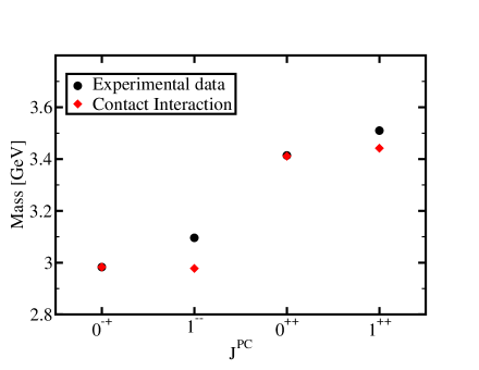
Figure 1: Contact interaction results for the $\overline{c}c$ mass spectrum using model parameters fitted in the light sector, see Table 3 PDG-labeled data is from  Nakamura and Group (2010).

VI.1 Charmonia mass spectrum

It has been shown Gutierrez-Guerrero et al. (2010); Roberts et al. (2010); Chen et al. (2012); Roberts et al. (2011a) that a momentum-independent vector$\times$vector interaction is capable of providing a description of light pseudoscalar and vector mesons static properties which is comparable to that obtained using more sophisticated QCD model interactions  Bashir et al. (2012b); Eichmann et al. (2008); Maris (2007); Cloet et al. (2007). Here we assess the capability of this model to provide a description of static properties of charmonia. The parameter set used in this calculation is the same as that obtained used in the light sector. Only the current-quark mass for the charm quark is an input parameter, and it is fixed such that the experimental mass of the pseudoscalar is reproduced. The rest of the meson masses are predictions of the model. As can be seen from Table 3, the predictions for the masses of the remaining mesons are in good agreement with the results obtained from more sophisticated SDE-BSE model calculations Blank and Krassnigg (2011); Rojas et al. (2014), lattice QCD for the charm sector Follana et al. (2007); Kalinowski and Wagner (2014) as well as experimental values Nakamura and Group (2010).

That a RL truncation with a CI describes well the mass spectrum of ground state charmonia can be understood in a simple way. Since the wave function renormalization and quark mass function are momentum-independent the heavy quark-gluon vertex can therefore reasonably be approximated by a bare vertex, ensuring the vector and axWTI.

VI.2 Decay constants

	amplitudes
	$\eta_{c}(1S)$	$J/\Psi(1S)$	$\chi_{c_{0}}(1P)$	$\chi_{c_{1}}(1P)$
$E_{H}$	6.028	3.024	0.437	0.298
	-	-	1.905	1.153
$F_{H}$	1.711	-	-	-
	decay constants
Experiment  Nakamura and Group (2010)	0.361	0.416	-	-
Contact Interaction	0.084	0.080	-	-

Table 4: Ground state charmonia amplitudes and decay constants obtained with the light sector parameter set adopted in Table 3:

Since the BSE is a homogeneous equation, the BSA has to be normalized by a separate condition. In the Rainbow-Ladder truncation of the BSE, that condition takes a simple form (we choose $\eta=1$):

$$\hskip 5.69046ptP_{\mu}=N_{c}\frac{\partial}{\partial P_{\mu}}\int\frac{\mathrm{d}^{4}q}{(2\pi)^{4}}\,\text{Tr}\left[\overline{\Gamma}_{H}(-Q)S(q_{+})\Gamma_{H}(Q)S(q)\right]\,,$$ (36)

at $Q=P$, with $P^{2}=-m_{H}^{2}$, which ensures that the residue at the mass pole is unity. Here, $\Gamma_{H}$ is the normalized BSA and $\overline{\Gamma}_{H}$ its charge conjugated version.

For every channel, we will re-scale $\Gamma_{H}$ such that Eq. (36) is satisfied. Thus, we replace $\Gamma_{H}$ with $\Gamma_{H}/N_{H}$, where $N_{H}$ is the normalization constant and now $\Gamma_{H}$ is the non-normalized BSA, the amplitude that is obtained by solving the homogeneous BSE. Thus the normalization constant is obtained from

$$N_{H}^{2}P^{2}=N_{c}P_{\mu}\frac{\partial}{\partial P_{\mu}}\int\frac{\mathrm{d}^{4}q}{(2\pi)^{4}}\,\text{Tr}\left[\overline{\Gamma}_{H}(-Q)S(q_{+})\Gamma_{H}(Q)S(q)\right]\,,$$ (37)

at $Q=P$, with $P^{2}=-m_{H}^{2}$. For the vector and axial vector channels there is an additional factor of $1/3$ on the right hand side since we have to take into account all three meson polarizations.

Once the BSA has been normalized canonically, we can calculate observables from it. The pseudoscalar leptonic decay constant, $f_{0^{-+}}$, is defined by (in a more realistic interaction, there is a factor of $Z_{2}$ on the right-hand side, and of course the BSA depends on the relative momentum)

$$P_{\mu}f_{0^{-+}}=N_{c}\int\frac{\mathrm{d}^{4}q}{(2\pi)^{4}}\,\text{Tr}\left[\gamma_{5}\gamma_{\mu}S(q_{+})\Gamma_{0^{-+}}(P)S(q_{-})\right]\,.$$ (38)

Similarly, the vector decay constant, $f_{1^{--}}$, is defined by

$$m_{1^{--}}f_{1^{--}}=\frac{N_{c}}{3}\int\frac{\mathrm{d}^{4}q}{(2\pi)^{4}}\,\text{Tr}\left[\gamma_{\mu}S(q_{+})\Gamma_{\mu 1^{--}}S(q_{-})\right]\,,$$ (39)

where $m_{1^{--}}$ is the mass of the $1^{--}$ bound state, and the factor of $3$ in the denominator comes from summing over the three polarizations of the spin-1 meson. Explicit expressions for the normalization condition in every channel and the decay constants $f_{0^{-+}}$ and $f_{1^{--}}$ are given in Appendix B.

As can be seem from Table 4, the pseudoscalar and vector decay constants, for the model parameters used, are strongly underestimated, in disagreement both with model calculations and experimental data. Numerically, this is because the corresponding BSAs are too small. Changing $\Lambda_{\text{UV}}$, e.g., to $1.843\,\text{GeV}$, keeping the other parameters fixed, except for the current-quark masses, which are taken from Ref. Nakamura and Group (2010), improves the situation by about a factor of $2$. However, there is still a significant mismatch between our results, model calculations, and experiment. We observe that this disagreement persists despite the fact that our calculation for the pseudoscalars are in perfect agreement with the Gell-Mann–Oakes–Renner relation, which is valid for every $0^{-}$ meson, irrespective of the magnitude of the current-quark mass, Krassnigg (2008); Holl et al. (2004); Blank and Krassnigg (2011).

It is not difficult to understand why the decay constants come out to be much smaller than what one expects from the QCD based SDE with running quark mass function. As noticed in Refs. Bhagwat et al. (2004); Maris and Roberts (1997); Maris and Tandy (1999), the decay constant is influenced by the high momentum tails of the dressed-quark propagator and the BSAs. This high momentum region probes the wave-function of quarkonia at origin. The CI, on the other hand, yields constant mass with no perturbative tail for large momenta. Therefore, this artefact of quarkonia has to be built into the model in an alternative manner. We know that with increasing mass of the heavy quarks, they become increasingly point-like in the configuration space. The closer the quarks get, the further the coupling strength between them decreases. Therefore, we cannot expect the decay constants to be correctly reproduced with the parameters of the light quark sector. In the next section, we consider the possibility of extending the simple CI model to the heavy sector by reducing the effective coupling. However, the reduction in the strength of the kernel has to be compensated by increasing the ultraviolet cut-off. This makes sense by observing that the $\Lambda_{\text{UV}}$ (highest energy scale associated with the system) used in the light quark sector is, in fact, less than the current charm quark mass. Therefore, it needs to be modified. We look for a balance between the effective coupling and the ultraviolet cut-off to describe the static properties of charmonia.

VII Contact Interaction Model for Charmonia

As we mentioned in the last section, we set out to redefine the parameters of the CI to study the masses, weak decay constants and the charge radii of charmonia.

	masses
	$m_{\eta_{c}(1S)}$	$m_{J/\Psi(1S)}$	$m_{\chi_{c_{0}}(1P)}$	$m_{\chi_{c_{1}}(1P)}$
Experiment  Nakamura and Group (2010)	2.983	3.096	3.414	3.510
Contact Interaction	2.950∗	3.129	3.407	3.433
			3.194	3.254
JM  Jain and Munczek (1993)	2.821	3.1	3.605	-
BK  Blank and Krassnigg (2011)	2.928	3.111	3.321	3.437
RB1  Rojas et al. (2014)	3.065	-	-	-
RB2  Rojas et al. (2014)	3.210	-	-	-

Table 5: Ground state charmonia masses obtained with the best-fit parameter set: $m_{g}=0.8\,\text{GeV}$, $\alpha_{IR}=0.93\pi/20$, $\Lambda_{\text{IR}}=0.24\,\text{GeV}$, $\Lambda_{\text{UV}}=2.788\,\text{GeV}$. The current-quark mass is $m_{c}=0.956^{*}\,\text{GeV}$, and the dynamically generated constituent-like mass is $M_{c}=1.497\,\text{GeV}$. The value immediately below the CI results is obtained without a spin-orbit coupling $g_{so}=0.24/3$. Dimensioned quantities are in GeV. (${}^{*}=$ This parameter set was obtained from a best-fit to the mass and decay constant of the pseudoscalar and vector channels).

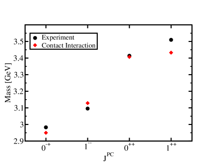
Figure 2: Contact interaction results for the $\overline{c}c$ mass spectrum, see Table 5. PDG-labelled data is taken from Ref. Nakamura and Group (2010).

We retain the parameters $m_{g}$ and $\Lambda_{\text{IR}}$ of the light sector. Modern studies of the gluon propagator indicate that in the infrared, the dynamically generated gluon mass scale virtually remains unaffected by the introduction of heavy dynamical quark masses, see for example Refs. Ayala et al. (2012); Bashir et al. (2013). The rest of the parameters are obtained from a best-fit to the mass and decay constant of the pseudoscalar ($\eta_{c}$) and vector ($J/\Psi$) channels.

One can now readily calculate the masses of the ground state pseudo-scalar, vector, scalar, and axial vector mesons. The results are shown in Table 5 and Fig. 2. They are in very good agreement with experimental values and comparable to the best SDE results with refined truncations. It is true that the masses of charmonia from quenched quark models can be shifted by large amounts when considering hadron loops, see e.g. Barnes and Swanson (2008). This observation appears to invalidate the quenched quark model results. However, as noted in Ref. Barnes and Swanson (2008), since this scale of mass shift is common to all low-lying states, it can therefore be absorbed in a change of model parameters. Thus, instead of consistently adding hadron loops into our Contact Interaction calculation, we have mimicked the effect by fitting the model parameters (coupling constant and ultraviolet cutoff). It ensures, for example, a constituent-like charm quark mass of the order of 1 GeV and a correct value for the experimental mass of the $\eta_{c}$.

For the case of the $\chi_{c_{1}}$, we find a mass of 3.254 GeV without a spin-orbit coupling, which is $7\%$ lower than the experimental value; our calculated value is even closer to that of the experimental $J/\psi$ mass. A similar pattern is observed with the pseudoscalar and scalar channels. Therefore, to achieve an acceptable mass difference between parity partners, we have introduced a spin-orbit coupling of $g_{SO}=0.08$. This gives the values in the second row of Table 5. As can be seen from the these values, the mass of the $\chi_{c_{1}}$ has increased only by $5\%$. This small effect is in line with the heavy-quark spin symmetry results. The spin-dependent interactions are proportional to the chromomagnetic moment of the quark (simulated by a spin orbit coupling). Predictably, these effects are substantially suppressed for charmonia as compared to light mesons.

The decay constants for the $\eta_{c}(1S)$ and $J/\Psi(1S)$ channels are reported in Table 6. For the pseudoscalar meson, the result aligns nicely with the experimental value. However, this is not exactly the case for the vector channel. Furthermore, we note that the decay constant for $J/\Psi(1S)$ is smaller than that for $\eta_{c}(1S)$. The correct ordering can be recovered by reducing the interaction strength by a large factor. However, this is something we consider contrived and, therefore, not pursue further. Notice that one of the SDE results yields the $J/\Psi(1S)$ decay constant even smaller than our value, Souchlas (2010).

	decay constants
	$f_{\eta_{c}}$	$f_{J/\Psi}$
Experiment  Nakamura and Group (2010)	0.361	0.416
S1rp  Souchlas (2010)	0.239	0.198
S3ccp  Souchlas (2010)	0.326	0.330
BK  Blank and Krassnigg (2011)	0.399	0.448
Contact Interaction	0.305	0.220

Table 6: The decay constants for the states $\eta_{c}(1S)$ and $J/\Psi(1S)$ obtained with $m_{g}=0.8\,\text{GeV}$, $\alpha_{IR}=0.93\pi/20$, $\Lambda_{\text{IR}}=0.24\,\text{GeV}$, $\Lambda_{\text{UV}}=2.788\,\text{GeV}$. The current-quark mass is $m_{c}=0.956\,\text{GeV}$. Dimensioned quantities are in GeV.

	$\eta_{c}(1S)$ charge radius
	SDE Bhagwat et al. (2007)	Lattice  Dudek et al. (2007)	CI
	0.219 fm	0.25 fm	0.21 fm

Table 7: The charge radius for the state $\eta_{c}(1S)$ obtained with the new parameter set discussed in the text.

As another test for the new parameter set for the CI Model for charmonia, we compute the charge radius of the $\eta_{c}(1S)$, $r^{2}_{\eta_{c}}=-6\partial F_{\eta_{c}}(Q^{2})/\partial Q^{2}|_{Q^{2}=0}$ where $F_{\eta_{c}}(Q^{2})$ is its electromagnetic form factor which we will report elsewhere and compare it with the results presented in Ref. Bhagwat et al. (2007) from previous SDE studies and Refs. Bhagwat et al. (2007); Dudek et al. (2007) from Lattice QCD. The results are presented in Table 7. As can be seen, our calculated charge radius is very close to the one obtained by employing the Maris-Tandy Model and the one reported in the lattice studies Bhagwat et al. (2007); Dudek et al. (2007).

VIII Conclusions

We compute the quark model ground state spin-0 and spin-1 charmonia masses and decay constants using a rainbow-ladder truncation of the simultaneous set of SDE and BSE with a CI model of QCD, developed and tested for the light quark sector Gutierrez-Guerrero et al. (2010); Roberts et al. (2010); Chen et al. (2012); Roberts et al. (2011a, b). As the model is non-renormalizable, we employ proper time regularization scheme which ensures confinement is implemented through the absence of quark production threshold. Moreover, the relevant Ward identities and the low energy theorems such as Goldberger-Triemann relations are satisfied. Without parameter readjustment, we find that the masses of the studied mesons are in reasonably good agreement with experimental data and other model calculations. Moreover, the Gell-Mann–Oakes–Renner relation, valid for every current-quark mass in the pseudo-scalar channel, is always satisfied. However, the decay constants of pseudo-scalar as well as vector mesons are significantly underestimated.

We realize that the extension of the CI model to the heavy sector requires a reduction of the effective coupling, which mimics the high momentum tail of the quark mass function obtained in the SDE studies of QCD Bhagwat et al. (2004); Maris and Roberts (1997); Maris and Tandy (1999). We only have to ensure that the reduction in the strength of the kernel is appropriately compensated by increasing the ultraviolet cut-off, a natural requirement for studying heavy quarks. We find that with a modified choice of two parameters, not only the masses of the ground state mesons, i.e., pseudo-scalar ($\eta_{c}(1S)$), vector ($J/\Psi(1S)$), scalar ($\chi_{c_{0}}(1P)$), and axial vector ($\chi_{c_{1}}(1P)$), but also their weak decay constants, are in much better agreement with the experiments Nakamura and Group (2010) as well as earlier SDE calculations with QCD based refined truncations Blank and Krassnigg (2011). As a further test of the model, we evaluate the charge radius of $\eta_{c}(1S)$ and found it reasonably close to the results computed in Refs. Bhagwat et al. (2007); Dudek et al. (2007). This is an encouraging first step towards a comprehensive study of heavy mesons in this approach. Further steps will involve flavored mesons and baryons. Our goal is to provide a unified description of light and heavy hadrons within the CI model.

Appendix A BSE Kernels

Here we give explicit expressions for the kernel in every channel considered in this article. The general expression for the kernel of matrix elements is

$$\mathcal{K}^{ij}_{H} = -\frac{4}{3}\frac{1}{m_{G}^{2}}\int\frac{\mathrm{d}^{4}q}{(2\pi)^{4}}\,\frac{\text{Tr}\left[\mathcal{P}^{i}_{H}(P)\gamma_{\mu}\hat{S}_{f}(q_{+})\mathcal{D}^{j}_{H}(P)\hat{S}_{g}(q_{-})\gamma_{\mu}\right]}{(q_{+}^{2}+M_{f}^{2})(q^{2}+M_{g}^{2})}$$

$$= -\frac{4}{3}\frac{1}{m_{G}^{2}}\int_{0}^{1}\mathrm{d}x\,\int\frac{\mathrm{d}^{4}q}{(2\pi)^{4}}\,\frac{\text{Tr}\left[\mathcal{P}^{i}_{H}(P)\gamma_{\mu}\hat{S}_{f}(q_{+})\mathcal{D}^{j}_{H}(P)\hat{S}_{g}(q_{-})\gamma_{\mu}\right]_{q\to q-xP}}{(q^{2}+\mathfrak{M}^{2})^{2}}\,,$$

where $\hat{S}_{f}(k)=-\mathrm{i}\gamma\cdot k+M_{f}$, and $\mathcal{D}_{H}^{i}$, $\mathcal{P}_{H}^{i}$ are, respectively, suitable Dirac covariants projectors for a given channel. In order to write compact expressions below, we define the following expressions

$$J(x) =x(1-x)\,, K(x) =M_{f}x+M_{g}(1-x)\,,$$

$$L(x) =M_{f}^{2}x+M_{g}^{2}(1-x)\,, L^{\pm}(x) =M_{f}M_{g}\pm L(x)\,.$$

For notational simplicity, we shall omit an overall factor of ${1}/{3\pi^{2}m_{G}^{2}}$ which multiplies the kernel in every channel.

A.1 Pseudoscalar kernel

For the pseudoscalar channel,

$$\mathcal{D}^{1}_{0^{-+}} =\mathrm{i}\gamma_{5}\,, \mathcal{D}^{2}_{0^{-+}} =\frac{1}{2M}\gamma_{5}\gamma\cdot P\,,$$ (41)

$$\mathcal{P}^{1}_{0^{-+}} =-\frac{\mathrm{i}}{4}\gamma_{5}\,, \mathcal{P}^{2}_{0^{-+}} =-\frac{M}{2P^{2}}\gamma_{5}\gamma\cdot P\,.$$ (42)

Thus

$$\mathcal{K}^{11}_{0^{-+}}=\int_{0}^{1}\mathrm{d}x\,\left[\mathcal{C}_{01}(\mathfrak{M}^{2})+\left(L^{-}(x)-2J(x)P^{2}\right)\mathcal{C}_{02}(\mathfrak{M}^{2})\right],$$

(43)

$$\mathcal{K}^{12}_{0^{-+}}=\frac{P^{2}}{2M}\int_{0}^{1}\mathrm{d}x\,K(x)\mathcal{C}_{02}(\mathfrak{M}^{2})\,,$$ (44)

$$\mathcal{K}^{21}_{0^{-+}}=M\int_{0}^{1}\mathrm{d}x\,K(x)\mathcal{C}_{02}(\mathfrak{M}^{2})\,,$$ (45)

$$\mathcal{K}^{22}_{0^{-+}}=-\frac{1}{2}\int_{0}^{1}\mathrm{d}x\,L^{+}(x)\mathcal{C}_{02}(\mathfrak{M}^{2})\,.$$ (46)

A.2 Vector kernel

For the vector channel,

$$\mathcal{D}^{1}_{1^{--}} =\gamma^{T}_{\mu}\,, \mathcal{D}^{2}_{1^{--}} =\frac{1}{2M}\sigma_{\mu\nu}P_{\nu}\,,$$ (47)

$$\mathcal{P}^{1}_{1^{--}} =\frac{1}{12}\gamma^{T}_{\mu}\,, \mathcal{P}^{2}_{1^{--}} =\frac{M}{6P^{2}}\sigma_{\mu\nu}P_{\nu}\,.$$ (48)

Thus

$$\mathcal{K}^{11}_{1^{--}}=\frac{1}{2}\int_{0}^{1}\mathrm{d}x\,(L^{-}(x)-2J(x)P^{2})\mathcal{C}_{02}(\mathfrak{M}^{2})\,,$$ (49)

$$\mathcal{K}^{12}_{1^{--}}=-\frac{P^{2}}{4M}\int_{0}^{1}\mathrm{d}x\,K(x)\mathcal{C}_{02}(\mathfrak{M}^{2})\,,$$ (50)

$$\mathcal{K}^{21}_{1^{--}}=0\,,$$ (51)

$$\mathcal{K}^{22}_{1^{--}}=0\,.$$ (52)

A.3 Scalar kernel

For the scalar channel,

$$\mathcal{D}^{1}_{0^{++}} = \mathbb{1}\,,$$ (53)

$$\mathcal{P}^{1}_{0^{++}} = \frac{1}{4}\mathbb{1}\,.$$ (54)

Thus

$$\mathcal{K}^{11}_{0^{++}}=\int_{0}^{1}\mathrm{d}x\,\left[\mathcal{C}(\mathfrak{M}^{2})-(L^{+}(x)+2J(x)P^{2})\mathcal{C}_{02}(\mathfrak{M}^{2})\right]\,.$$

A.4 Axial vector kernel

For the axial vector channel,

$$\mathcal{D}^{1}_{1^{++}} =\gamma_{5}\gamma^{T}_{\mu}\,, \mathcal{D}^{2}_{1^{++}} =\gamma_{5}\frac{1}{2M}\sigma_{\mu\nu}P_{\nu}\,,$$ (56)

$$\mathcal{P}^{1}_{1^{++}} =\frac{1}{12}\gamma^{T}_{\mu}\gamma_{5}\,, \mathcal{P}^{2}_{1^{++}} =\frac{M}{6P^{2}}\sigma_{\mu\nu}P_{\nu}\gamma_{5}\,.$$ (57)

Thus

$$\mathcal{K}^{11}_{1^{++}} = -\frac{1}{2}\int_{0}^{1}\mathrm{d}x\,(L^{+}(x)+2J(x)P^{2})\mathcal{C}_{02}(\mathfrak{M}^{2})\,,$$

$$\mathcal{K}^{12}_{1^{++}} = 0\,,$$ (59)

$$\mathcal{K}^{21}_{1^{++}} = 0\,,$$ (60)

$$\mathcal{K}^{22}_{1^{++}} = 0\,.$$ (61)

Appendix B Normalization

In the appendix, we give explicit expressions for normalization condition in every channel considered and for the decay constants of pseudoscalar and vector mesons. The general expression for the normalization condition can be written as

$$N_{H}^{2}=\sum\limits_{i,j=1}\mathcal{N}^{ij}_{H}\mathcal{F}^{i}_{H}\mathcal{F}^{j}_{H}\,,$$ (62)

where the upper limits on the summations depend on the number of non zero dressing functions in a given channel. A factor of $1/16\pi^{2}$ multiplies every $\mathcal{N}^{ij}_{H}$ and recall the factor of $1/3$ for the vector and axial vector channels, stemming from all three polarizations.

B.1 Pseudoscalar channel

In this channel, the normalizations are:

$$\mathcal{N}^{11}_{0^{-+}}=~{}~{}~{}8~{}~{}~{}\int_{0}^{1}\mathrm{d}x\,J(x) \left[2\left(L^{-}(x)-2J(x)P^{2}\right)\mathcal{C}_{03}(\mathfrak{M}^{2})\right.$$

$$\left.+3\mathcal{C}_{02}(\mathfrak{M}^{2})\right]\,,$$ (63)

$$\mathcal{N}^{12}_{0^{-+}}=-\frac{2}{M}\int_{0}^{1}\mathrm{d}x\,K(x) \left[-4J(x)P^{2}\mathcal{C}_{03}(\mathfrak{M}^{2})\right.$$

$$\left.+\mathcal{C}_{02}(\mathfrak{M}^{2})\right]\,,$$ (64)

$$\mathcal{N}^{21}_{0^{-+}}=-\frac{2}{M}\int_{0}^{1}\mathrm{d}x\,K(x) \left[-4J(x)P^{2}\mathcal{C}_{03}(\mathfrak{M}^{2})\right.$$

$$\left.+\mathcal{C}_{02}(\mathfrak{M}^{2})\right]\,,$$ (65)

$$\mathcal{N}^{22}_{0^{-+}}=-\frac{4P^{2}}{M^{2}}\int_{0}^{1}\mathrm{d}x\,J(x) L^{+}(x)\mathcal{C}_{03}(\mathfrak{M}^{2})\,.$$ (66)

B.1.1 Pseudoscalar decay constant

Explicit expression for the decay constant is as follows:

$$f_{0^{-}} = N_{c}\left[\mathcal{K}_{0^{-}}^{1}\mathcal{F}^{1}_{0^{-}}+\mathcal{K}_{0^{-}}^{2}\mathcal{F}^{2}_{0^{-}}\right]\,,$$ (67)

$$\mathcal{K}_{0^{-}}^{1} = \frac{1}{16\pi^{2}}\int_{0}^{1}\mathrm{d}x\,K(x)\mathcal{C}_{02}(\mathfrak{M}^{2})\,,$$

$$\mathcal{K}_{0^{-}}^{1} = -\frac{1}{16\pi^{2}}\frac{2}{M}\int_{0}^{1}\mathrm{d}x\,L^{+}(x)\mathcal{C}_{02}(\mathfrak{M}^{2})\,.$$

B.2 Vector channel

The normalization condition in this channel is:

$$\mathcal{N}^{11}_{1^{--}}=48\int_{0}^{1}\mathrm{d}x\,J(x)\left[\left(L^{-}(x)-2J(x)P^{2}\right)\mathcal{C}_{03}(\mathfrak{M}^{2})\right.\\ +\left.\mathcal{C}_{02}(\mathfrak{M}^{2})\right]\,.$$ (68)

B.2.1 Vector decay constant

The vector decay constant is given by:

$$f_{1^{--}} = \frac{N_{c}}{3m_{1^{--}}}\mathcal{K}_{1^{--}}^{1}\mathcal{F}^{1}_{1^{--}}\,,$$ (69)

$$\mathcal{K}_{1^{--}}^{1} = \frac{12}{16\pi^{2}}\int_{0}^{1}\mathrm{d}x\,\left(L^{-}(x)-2J(x)P^{2}\right)\mathcal{C}_{02}(\mathfrak{M}^{2})\,.$$

B.3 Scalar channel

The normalization condition in this channel is:

$$\mathcal{N}^{11}_{0^{++}}=8\int_{0}^{1}\mathrm{d}x\,J(x)\left[-\left(L^{+}(x)+2J(x)P^{2}\right)\mathcal{C}_{02}(\mathfrak{M}^{2})\right.\\ +\left.3\mathcal{C}_{02}(\mathfrak{M}^{2})\right]\,.$$ (70)

B.4 Axial vector channel

The normalization condition for the axial vector channel is:

$$\mathcal{N}^{11}_{1^{++}}=48\int_{0}^{1}\mathrm{d}x\,J(x)\left[\left(L^{+}(x)+2J(x)P^{2}\right)\mathcal{C}_{03}(\mathfrak{M}^{2})\right.\\ -\left.\mathcal{C}_{02}(\mathfrak{M}^{2})\right]\,.$$ (71)

References

- Jain and Munczek (1993) P. Jain and H. J. Munczek, Phys.Rev. D48, 5403 (1993), eprint hep-ph/9307221.
- Maris et al. (1998) P. Maris, C. D. Roberts, and P. C. Tandy, Phys. Lett. B420, 267 (1998), eprint nucl-th/9707003.
- Maris and Tandy (1999) P. Maris and P. C. Tandy, Phys. Rev. C60, 055214 (1999), eprint nucl-th/9905056.
- Boucaud et al. (2008) P. Boucaud, J. Leroy, A. Le Yaouanc, J. Micheli, O. Pene, et al., JHEP 0806, 099 (2008), eprint 0803.2161.
- Aguilar et al. (2008) A. Aguilar, D. Binosi, and J. Papavassiliou, Phys.Rev. D78, 025010 (2008), eprint 0802.1870.
- Pennington and Wilson (2011) M. Pennington and D. Wilson, Phys.Rev. D84, 119901 (2011), eprint 1109.2117.
- Chang and Roberts (2009) L. Chang and C. D. Roberts, Phys.Rev.Lett. 103, 081601 (2009), eprint 0903.5461.
- Kizilersu and Pennington (2009) A. Kizilersu and M. Pennington, Phys.Rev. D79, 125020 (2009), eprint 0904.3483.
- Bashir et al. (2012a) A. Bashir, R. Bermudez, L. Chang, and C. Roberts, Phys.Rev. C85, 045205 (2012a), eprint 1112.4847.
- Krassnigg and Maris (2005) A. Krassnigg and P. Maris, J.Phys.Conf.Ser. 9, 153 (2005), eprint nucl-th/0412058.
- Bhagwat et al. (2007) M. Bhagwat, A. Krassnigg, P. Maris, and C. Roberts, Eur.Phys.J. A31, 630 (2007), eprint nucl-th/0612027.
- Maris and Tandy (2006) P. Maris and P. Tandy, Nucl.Phys.Proc.Suppl. 161, 136 (2006), eprint nucl-th/0511017.
- Blank and Krassnigg (2011) M. Blank and A. Krassnigg, Phys.Rev. D84, 096014 (2011), eprint 1109.6509.
- Maris (2007) P. Maris, AIP Conf.Proc. 892, 65 (2007), eprint nucl-th/0611057.
- Krassnigg (2009) A. Krassnigg, Phys.Rev. D80, 114010 (2009), eprint 0909.4016.
- Bhagwat et al. (2004) M. Bhagwat, A. Holl, A. Krassnigg, C. Roberts, and P. Tandy, Phys.Rev. C70, 035205 (2004), eprint nucl-th/0403012.
- Souchlas (2010) N. Souchlas, Phys.Rev. D81, 114019 (2010).
- Rojas et al. (2014) E. Rojas, B. El-Bennich, and J. de Melo, Phys.Rev. D90(7), 074025 (2014), eprint 1407.3598.
- Gutierrez-Guerrero et al. (2010) L. Gutierrez-Guerrero, A. Bashir, I. Cloet, and C. Roberts, Phys.Rev. C81, 065202 (2010), eprint 1002.1968.
- Roberts et al. (2010) H. Roberts, C. Roberts, A. Bashir, L. Gutierrez-Guerrero, and P. Tandy, Phys.Rev. C82, 065202 (2010), eprint 1009.0067.
- Chen et al. (2012) C. Chen, L. Chang, C. D. Roberts, S. Wan, and D. J. Wilson, Few Body Syst. 53, 293 (2012), eprint 1204.2553.
- Roberts et al. (2011a) H. L. Roberts, L. Chang, I. C. Cloet, and C. D. Roberts, Few Body Syst. 51, 1 (2011a), eprint 1101.4244.
- Roberts et al. (2011b) H. Roberts, A. Bashir, L. Gutierrez-Guerrero, C. Roberts, and D. Wilson, Phys.Rev. C83, 065206 (2011b), eprint 1102.4376.
- Bashir et al. (2012b) A. Bashir, L. Chang, I. C. Cloet, B. El-Bennich, Y.-X. Liu, et al., Commun.Theor.Phys. 58, 79 (2012b), eprint 1201.3366.
- Eichmann et al. (2008) G. Eichmann, R. Alkofer, I. Cloet, A. Krassnigg, and C. Roberts, Phys.Rev. C77, 042202 (2008), eprint 0802.1948.
- Cloet et al. (2007) I. Cloet, A. Krassnigg, and C. Roberts, eConf C070910, 125 (2007), eprint 0710.5746.
- Gross (1993) F. Gross, Relativistic quantum mechanics and field theory (Wiley, New York, 1993), first ed.
- Salpeter and Bethe (1951) E. E. Salpeter and H. A. Bethe, Phys. Rev. 84, 1232 (1951).
- Gell-Mann and Low (1951) M. Gell-Mann and F. Low, Phys. Rev. 84, 350 (1951).
- Roberts et al. (2007) C. D. Roberts, M. S. Bhagwat, A. Holl, and S. V. Wright, Eur. Phys. J. ST 140, 53 (2007), eprint 0802.0217.
- Holl et al. (2006) A. Holl, C. D. Roberts, and S. V. Wright (2006), eprint nucl-th/0601071.
- Maris and Roberts (2003) P. Maris and C. D. Roberts, Int. J. Mod. Phys. E12, 297 (2003), eprint nucl-th/0301049.
- Alkofer and von Smekal (2001) R. Alkofer and L. von Smekal, Phys. Rept. 353, 281 (2001), eprint hep-ph/0007355.
- Boucaud et al. (2012) P. Boucaud, J. Leroy, A. L. Yaouanc, J. Micheli, O. Pene, et al., Few Body Syst. 53, 387 (2012), eprint 1109.1936.
- Ebert et al. (1996) D. Ebert, T. Feldmann, and H. Reinhardt, Phys.Lett. B388, 154 (1996), eprint hep-ph/9608223.
- Roberts (2008) C. Roberts, Prog.Part.Nucl.Phys. 61, 50 (2008), eprint 0712.0633.
- Farias et al. (2006) R. Farias, G. Dallabona, G. Krein, and O. Battistel, Phys.Rev. C73, 018201 (2006), eprint hep-ph/0510145.
- Farias et al. (2008) R. Farias, G. Dallabona, G. Krein, and O. Battistel, Phys.Rev. C77, 065201 (2008), eprint hep-ph/0604203.
- Weise (2005) W. Weise (2005), eprint nucl-th/0504087.
- Fischer et al. (2007) C. S. Fischer, D. Nickel, and J. Wambach, Phys. Rev. D76, 094009 (2007), eprint 0705.4407.
- Munczek (1995) H. J. Munczek, Phys. Rev. D52, 4736 (1995), eprint hep-th/9411239.
- Cornwall et al. (1974) J. M. Cornwall, R. Jackiw, and E. Tomboulis, Phys. Rev. D10, 2428 (1974).
- Llewellyn-Smith (1969) C. H. Llewellyn-Smith, Ann. Phys. 53, 521 (1969).
- Nakamura and Group (2010) K. Nakamura and P. D. Group, Journal of Physics G: Nuclear and Particle Physics 37(7A), 075021 (2010), URL http://stacks.iop.org/0954-3899/37/i=7A/a=075021.
- Follana et al. (2007) E. Follana et al. (HPQCD Collaboration, UKQCD Collaboration), Phys.Rev. D75, 054502 (2007), eprint hep-lat/0610092.
- Kalinowski and Wagner (2014) M. Kalinowski and M. Wagner, PoS LATTICE2013, 241 (2014), eprint 1310.5513.
- Krassnigg (2008) A. Krassnigg, PoS CONFINEMENT8, 075 (2008), eprint 0812.3073.
- Holl et al. (2004) A. Holl, A. Krassnigg, and C. D. Roberts, Phys. Rev. C70, 042203 (2004), eprint nucl-th/0406030.
- Maris and Roberts (1997) P. Maris and C. D. Roberts, Phys. Rev. C56, 3369 (1997), eprint nucl-th/9708029.
- Ayala et al. (2012) A. Ayala, A. Bashir, D. Binosi, M. Cristoforetti, and J. Rodriguez-Quintero, Phys.Rev. D86, 074512 (2012), eprint 1208.0795.
- Bashir et al. (2013) A. Bashir, A. Raya, and J. Rodriguez-Quintero, Phys.Rev. D88, 054003 (2013), eprint 1302.5829.
- Barnes and Swanson (2008) T. Barnes and E. S. Swanson, Phys. Rev. C77, 055206 (2008), eprint 0711.2080.
- Dudek et al. (2007) J. J. Dudek, R. G. Edwards, N. Mathur, and D. G. Richards, J.Phys.Conf.Ser. 69, 012006 (2007).