Abstract

We report the discovery of a partial conservation law obeyed by a schematic Hamiltonian of two protons and two neutrons in a $j$ shell. In our Hamiltonian the interaction matrix element of two nucleons with combined angular momentum $J$ is linear in $J$ for even $J$ and constant for odd $J$. It turns out that in some stationary states the sum of the angular momenta $J_{p}$ and $J_{n}$ of the proton and neutron pairs is conserved. The energies of these states are given by a linear function of $J_{p}+J_{n}$. The systematics of their occurrence is described and explained.

Chapter 0 Partial Conservation Law in a Schematic Single $j$ Shell Model

1 Introduction

Among the many contributions of Gerry Brown to Nuclear Physics one of the first that comes to the minds of many is his development with Tom Kuo of realistic nuclear matrix elements.[1] These involve the very complicated nucleon nucleon interaction and the added complication of handling the hard core by obtaining a $G$ matrix which a researcher could easily handle. However our present work is inspired by another aspect of Gerry Brown’s contributions—his use of simple schematic models to bring out the physics of the more complex calculations. One example is his early article with Marc Bolsterli in Physical Review Letter on dipole states in nuclei.[2] Their simple model employs a delta interaction with radial integrals set to a constant. One state gets elevated to a high energy and contains all the dipole strength. Gerry and Marc compared their results with a more detailed calculation of Elliott and Flowers.[3] These authors obtained two collective states, and Gerry and Marc noted that a defect of their model was the neglect of the spin orbit interaction. However they expected that it could work better for heavier nuclei. A quote from the end of their paper: “The schematic model is of course no substitute for detailed calculations but indicates the possibility of these coherent features in a simple way.”

In Gerry’s first book Unified Theory of Nuclear Models[4] he discusses besides more elaborate schemes of calculation such schematic models as Elliott’s SU(3) model to describe nuclear rotation[5] and Racah’s seniority scheme displaying the physics of pairing in nuclei.[6]

Below we consider a simple model with only one $j$ shell, where we put both protons and neutrons. Such a model was applied in the early days to the description of nuclear spectra, magnetic moments, beta deay etc. in the $1f_{7/2}$ shell.[7, 8, 9, 10, 11] The interaction matrix elements were taken from the spectra of ⁴²Ca and ⁴²Sc. The ⁴²Sc, $T=0$ spectrum was poorly known at that time and some of the assignments were wrong. Revised matrix elements were later extracted from the correct ⁴²Sc spectrum by Zamick and Robinson,[12] and these matrix elements were employed by Escuderos, Zamick and Bayman in complete calculations for the $1f_{7/2}$ shell.[13] Despite large differences between the original and revised matrix elements, especially a lowering of those for two nucleon angular momentum $J=1$, 3 and 5 by about half an MeV, no red flags were raised. This indicates a certain insensitivity to the $T=0$ matrix, a theme that will pervade this work.

Figure 1: Empirical interaction of two nucleons in the $1f_{7/2}$ shell derived from the spectrum of ⁴²Sc. The matrix elements $E^{J}$ are connected by broken lines separately for even and odd J. The dashed lines suggest an approximation of the even $J$ matrix elements by a function linear in $J$ and the odd $J$ matrix elements by a constant.

In our present investigation $j$ is arbitrary, and we adopt a schematic interaction. The nuclei considered are such which have two protons and two neutrons in the given shell. It is well known that such a model also applies to the case of two proton holes and two neutron holes. Our choice of schematic interaction is motivated by the gross structure of the matrix elements of Ref. 12, which are displayed in fig:42Sc. Shown there are the interaction matrix elements $E^{J}=\langle(jj)J|v|(jj)J\rangle$, where $j=7/2$. It is seen that while the even $J$ matrix element rises steeply with $J$, the odd $J$ matrix element varies much less and its average slope as a function of $J$ is approximately zero. This suggests to approximate the even $J$ matrix elements by a function linear in $J$ and the odd $J$ matrix elements by a constant $c$. The only effect of this constant is to add $(3-\frac{1}{2}T(T+1))c$ to all energies, where $T$ is the total isospin. The stationary wave functions are not affected. As we consider only states with $T=0$, we can therefore choose $c=0$ just as well. The interaction then depends only on an energy scale factor. Choosing this scale factor in the simplest possible way we arrive at the following schematic interaction to be studied in the subsequent part of this chapter.

$$E^{J}=\begin{cases}J,&\text{even $J$,}\\ 0,&\text{odd $J$.}\end{cases}$$ (1)

The next section shows examples of results derived numerically from this interaction. We illustrate, in particular, the occurrence for certain values of $j$ and the total angular momentum $I$, of stationary states where the sum $J_{p}+J_{n}$ of the angular momenta of the proton and neutron pairs is conserved. We also illustrate that these states, which we call special states, always have absolute energies (that is, energies before the ground state energy is subtracted to give an excitation energy) equal to $3(J_{p}+J_{n})/2$. To finish the section we report a systematic search of special states for all $j\leq 15/2$ and give empiric rules for their occurrence. In sec:expl we then explain these observations, and the present chapter is summarised in sec:sum.

2 Numeric results

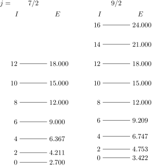
Figure 2: Calculated even $I$ yrast bands for $j=7/2$ and 9/2. The absolute energy $E$ of each level is indicated.

Figure 2 shows the even $I$ yrast bands calculated for $j=7/2$ and 9/2. The top half of each band is seen to be strictly linear. In fact the absolute energies equal $3I/2$. The wave functions, shown in tbl:9h_ywf for $j=9/2$, have a very simple structure. As all these states have $T=0$, which implies that the coefficient of a basic state

$$|J_{p}J_{n}\rangle=|((jj)J_{p}(jj)J_{n})IM\rangle,$$ (2)

acquires a sign factor $(-)^{I}$ when $J_{p}$ and $J_{n}$ are interchanged, we show in the table the coefficients of the basic states

$$|J_{p}J_{n}\rangle_{\text{e}}=2^{-\frac{1+\delta_{J_{p}J_{n}}}{2}}(|J_{p}J_{n}\rangle+(-)^{I}|J_{n}J_{p}\rangle).$$ (3)

All the states listed in tbl:9h_ywf are seen to have only components with $J_{p}+J_{n}=I$. In eq:—¿ the first two angular momenta $j$ are those of the individual protons and the last two those of the neutrons. The total magnetic quantum number $M$ is arbitrary. In eq:—¿e the angular momenta $J_{p}$ and $J_{n}$ are even, $J_{p}\geq J_{n}$ for even $I$ and $J_{p}>J_{n}$ for odd $I$. The subscript ‘e’ stands for ‘even’ to indicate that these states span the space where $T$ is even for the given $j$, $I$ and $M$. This is used in sec:expl.

Wave functions in the calculated even $I$ yrast band for $j=9/2$ and $I\geq 8$. Shown are the coeeficients of the states $|J_{p}J_{n}\rangle_{\text{e}}$ defined by eq:—¿e. $J_{p}$ $J_{n}$ $I=$ 8 10 12 14 16 4 4 0.595 6 2 0.700 6 4 0.000 0.885 6 6 0.000 0.000 0.745 8 0 0.395 8 2 0.000 0.466 8 4 0.000 0.000 0.667 8 6 0.000 0.000 0.000 1.000 8 8 0.000 0.000 0.000 0.000 1.000

Several other states are degenerate with these even $I$ yrast states. They are listed in tbl:9h_ny. All these states have $T=0$. As this holds for all the states discussed in this chapter, we do not mention it any more. Most of the states in tbl:9h_ny have odd $I$. The lowest state for each of $I=9$, 11 and 13 is an yrast state and degenerate with the yrast state with one unit higher angular momentum. (The only state with $I=15$, which as such is necessarily the yrast state for this angular momentum, has $T=1$.) Inspecting the wave functions, one notices again a conservation of $J_{p}+J_{n}$. Furthermore the energy is always $3(J_{p}+J_{n})/2$

Energies $E$ and wave functions of $j=9/2$ special states not belonging to the even $I$ yrast band. The wave functions are shown as coeeficients of the states $|J_{p}J_{n}\rangle_{\text{e}}$. $E=$ 15 15 18 18 21 21 24 $J_{p}$ $J_{n}$ $I=$ 7 9 10 11 11 13 14 6 2 0.000 6 4 0.872 0.459 0.000 6 6 0.689 8 0 0.000 8 2 -0.489 0.888 0.000 8 4 0.000 0.000 -0.725 1.000 0.000 8 6 0.000 0.000 0.000 0.000 1.000 1.000 0.000 8 8 0.000 1.000

An analogous situation emerges for any $j$ we have examined. Table 2 shows the result of a complete search of special states for $j\leq 15/2$. Always the absolute energy is $3(J_{p}+J_{n})/2$. The following systematics is inferred from tbl:search.

• For a given $j$ there is a special state for any $I$ from $2j-1$ to $4j-2$ except $4j-3$ (which is impossible for $j=1/2$ and accommodates for $j\geq 3/2$ just a single $T=1$ state). These states have $J_{p}+J_{n}=I$ for even $I$ and $J_{p}+J_{n}=I+1$ for odd $I$ and are yrast states.

• Besides, there are special states with $(J_{p}+J_{n},I)=(4j-8,4j-11)$, $(4j-6,4j-8)$, $(4j-4,4j-7)$ and $(4j-2,4j-4)$ provided this $I$ is not negative.

These rules have only two exceptions, both of which occur for fairly low $j$: First, there is no $(J_{p}+J_{n},I)=(4j-6,4j-8)=(4,2)$ special state for$j=5/2$. Second, there is an additional $(J_{p}+J_{n},I)=(10,3)=\linebreak(4j-4,4j-11)$ special state for $j=7/2$.

All special states occurring for $j\leq 15/2$. $j$ $J_{p}+J_{n}$ $I$ $j$ $J_{p}+J_{n}$ $I$ 1/2 0 0 13/2 12 12 3/2 2 2 14 13, 14 4 2, 4 16 15, 16 5/2 4 4 18 15, 17, 18 6 3, 5, 6 20 18, 19, 20 8 6, 8 22 19, 21, 22 7/2 6 3, 6 24 22, 24 8 6, 7, 8 15/2 14 14 10 3, 7, 9, 10 16 15, 16 12 10, 12 18 17, 18 9/2 8 8 20 19, 20 10 7, 9, 10 22 19, 21, 22 12 10, 11, 12 24 22, 23, 24 14 11, 13, 14 26 23, 25, 26 16 14, 16 28 26, 28 11/2 10 10 12 11, 12 14 11, 13, 14 16 14, 15, 16 18 15, 17, 18 20 18, 20

The four degenerate levels with $J_{p}+J_{n}=10$ and $I=3$, 7, 9 and 10 occurring for $j=7/2$ are familiar from studies by Robinson and Zamick[14, 15]. These authors consider an interaction in the $1f_{7/2}$ shell with $E^{J}=0$ for odd $J$ and arbitrary $E^{J}$ is for even $J$. (As noted in the introduction, their results then apply essentially unaltered to the case when $E^{J}$ is constant for odd $J$.) From properties of 9-$j$ symbols they derive in Ref. 14 that for these $I$ there is a stationary state whose wave function is just $|64\rangle_{\text{e}}$. Because for all these $I$ this is the only $|J_{p}J_{n}\rangle_{\text{e}}$ with $J_{p}+J_{n}=10$, these are the same states as considered presently. A slight extension of the arguments in Ref. 14 shows that for the more general interaction considered there they have energies $3(E^{6}+E^{4})/2$, so they are degenerate. In Ref. 15 the properties of 9-$j$ symbols employed in Ref. 14 are derived from the fact that none of the four angular momenta accomodate $T=2$. It is shown in sec:expl that when this happens and $E^{J}=0$ for odd $J$, then quite generally any $|J_{p}J_{n}\rangle_{\text{e}}$ is a stationary state. Its energy is $3(E^{J_{p}}+E^{J_{n}})/2$.

3 Explanation

How is it possible that $J_{p}+J_{n}$ is conserved in some stationary states of our schematic Hamiltonian, and why do these states always have energy$3(J_{p}+J_{n})/2$? In order to see how this comes about notice that for given $j$, $I$ and $M$ this Hamiltonian $H$ has matrix elements

$$\langle J_{p}J_{n}|H|J_{p}^{\prime}J_{n}^{\prime}\rangle=\delta_{J_{p}J_{p}^{\prime}}\delta_{J_{n}J_{n}^{\prime}}(E^{J_{p}}+E^{J_{n}})\\ +4\sum_{J_{1}J_{2}}\langle J_{p}J_{n}\|J_{1}J_{2}\rangle E^{J_{1}}\langle J_{1}J_{2}\|J_{p}^{\prime}J_{n}^{\prime}\rangle,$$ (4)

where $\langle J_{1}J_{2}\|J_{1}^{\prime}J_{2}^{\prime}\rangle$ is shorthand for a unitary 9-$j$ symbol,

$$\langle J_{1}J_{2}\|J_{1}^{\prime}J_{2}^{\prime}\rangle=\langle((j_{1}j_{2})J_{1}(j_{3}j_{4})J_{2})IM|((j_{1}j_{3})J_{1}^{\prime}(j_{2}j_{4})J_{2}^{\prime}))IM\rangle,$$ (5)

where all $j$’s equal $j$. While the angular momenta $J_{p}$, $J_{n}$, $J_{p}^{\prime}$ and $J_{n}^{\prime}$ are even, $J_{1}$ and $J_{2}$ take all values allowed by the triangle inequalities. It is convenient to define an operator $X$ such that

$$\langle J_{1}J_{2}|X|J_{1}^{\prime}J_{2}^{\prime}\rangle=\langle J_{1}J_{2}\|J_{1}^{\prime}J_{2}^{\prime}\rangle.$$ (6)

The space with even $T$ is spanned by the states $|J_{p}J_{n}\rangle_{\text{e}}$. By the symmetry of $\langle J_{p}J_{n}\|J_{1}J_{2}\rangle$ the matrix element $\langle J_{p}J_{n}|_{\text{e}}\,X|J_{1}J_{2}\rangle$ vanishes unless $J_{1}$ and $J_{2}$ have equal parities. Therefore, in the even $T$ space, when $E^{J}=0$ for odd $J$, only even $J_{1}$ and $J_{2}$ contribute to the sum in (4), and we have

$$H=\Omega+2W\Omega W$$ (7)

with operators $\Omega$ and $W$ acting within the even $T$ space and defined by

$$\langle J_{p}J_{n}|\Omega|J_{p}^{\prime}J_{n}^{\prime}\rangle_{\text{e}}=\delta_{J_{p}J_{p}^{\prime}}\delta_{J_{n}J_{n}^{\prime}}(E^{J_{p}}+E^{J_{n}}),$$ (8)

$$\langle J_{p}J_{n}|W|J_{p}^{\prime}J_{n}^{\prime}\rangle_{\text{e}}=\langle J_{p}J_{n}|X|J_{p}^{\prime}J_{n}^{\prime}\rangle_{\text{e}}.$$ (9)

The subscript ‘e’ indicates that the matrix element is taken between states $|J_{p}J_{n}\rangle_{\text{e}}$.

We denote by $(ik)$ the interchange of the states of the $i$th and $k$th nucleons, where the nucleons are numbered in the order of appearance of their angular momenta in eq:—¿. Due to $(12)|J_{p}J_{n}\rangle=(34)|J_{p}J_{n}\rangle=-|J_{p}J_{n}\rangle$ one can make in eq:W the substitution

$$4X=(13)+(14)+(23)+(24).$$ (10)

By Eq. (4) of Ref. 16 we have

$$\sum_{i<k}(ik)=4-4^{2}/4-T(T+1)=-T(T+1).$$ (11)

As a result the matrix $W$ has the eigenvalue $(-T(T+1)-2\times(-1))/4=1/2$ for $T=0$. In particular, if some $T=0$ state is an eigenstate of $\Omega$ it is an eigenstate of $H$ with eigenvalue $1+2\times(1/2)^{2}=3/2$ times that of $\Omega$.

This explains the finding of Robinson and Zamick in Ref. 15. If $T=2$ is not accomodated for the given $j$ and $I$ then the states $|J_{p}J_{n}\rangle_{\text{e}}$ have $T=0$. They are also eigenstates of $\Omega$ with eigenvalue $E^{J_{p}}+E^{J_{n}}$. Therefore they are eigenstates of $H$ with eigenvalue $3(E^{J_{p}}+E^{J_{n}})/2$.

For the Hamiltonian presently considered any linear combination of states $|J_{p}J_{n}\rangle_{\text{e}}$ with $J_{p}+J_{n}=k$, where $k$ is a constant, is an eigenstate of $\Omega$ with eigenvalue $k$. What then remains to be explained is that for the combinations of $j$, $k$ and $I$ obeying the above rules 1 and 2 with the two exceptions mentioned, there exist such linear combinations which have $T=0$. The rest of this section is devoted to a proof of this. The proof is divided into separate parts for the two rules. Notice that the second exception is explained already. The special state with $(j,k,I)=(7/2,10,3)$ is one of the states discussed by Robinson and Zamick in Refs. 14, 15. An explanation of the first exception is deferred to sec:rule2.

1 Rule 1

We discuss the cases of even and odd $I$ separately.

Even $I$

Let

$$|\psi\rangle=\sum_{J_{p}+J_{n}=k}c_{J_{p}}|(J_{p}J_{n})kk\rangle,$$ (12)

with some set of coefficients $c_{J}$, where we have included explicitly $I$ and $M$ on the left hand side of eq:—¿. This state evidently has $I=k$. We assume $k\geq 2j-1$, so the range $\mathcal{S}$ of $J_{p}$ in the summation is the set of even integers $J$ with $k-2j+1\leq J\leq 2j-1$. From formulas for vector coupling coefficients [17] one gets

$$\langle m_{1}m_{2}m_{3}m_{4}|\psi\rangle\mathrel{\mathop{:}}=(\langle jm_{1}|\times\langle jm_{2}|\times\langle jm_{3}|\times\langle jm_{4}|)\,|\psi\rangle\\ =\delta_{m_{1}+m_{2}+m_{3}+m_{4},k}(-)^{m_{1}-m_{3}}a(m_{1})a(m_{2})a(m_{3})a(m_{4})f(m_{1}+m_{2}),$$ (13)

where the $m$’s are single nucleon magnetic quantum numbers, and

$$a(m)=\sqrt{\frac{(j+m)!}{(j-m)!}},$$ (14)

$$f(\mu)=\begin{cases}b(\mu)b(k-\mu)c_{\mu},&\mu\in\mathcal{S},\\ 0,&\text{otherwise},\end{cases}$$ (15)

$$b(J)=\frac{1}{J!}\sqrt{\frac{(2j-J)!(2J+1)!}{(2j+J+1)!}}.$$ (16)

By eq:sumof() the state $|\psi\rangle$ has $T=0$ when it belongs to the kernel of

$$K=(13)+(14)+(23)+(24)-2.$$ (17)

This is seen to be equivalent to

$$(-)^{m_{3}-m_{1}}f(m_{3}+m_{2})+(-)^{m_{4}-m_{3}}f(m_{4}+m_{2})\\ +(-)^{m_{1}-m_{2}}f(m_{1}+m_{3})+(-)^{m_{1}-m_{3}}f(m_{1}+m_{4})\\ -2(-)^{m_{1}-m_{3}}f(m_{1}+m_{2})=0$$ (18)

for $m_{1}+m_{2}+m_{3}+m_{4}=k$. Equation (18) holds when $f(\mu)$ is constant for $\mu\in\mathcal{S}$. Indeed, when $m_{1}+m_{2}+m_{3}+m_{4}=k$, no sum $\mu$ of two of the $m$’s is greater that $2j$ or less than $k-2j$, so $\mu\in\mathcal{S}$ if $\mu$ is even. First assume that $m_{1}+m_{2}$ is even. If $m_{4}+m_{2}$ is even then the sign factor in the second term in eq:f-cond becomes $(-)^{m_{1}-m_{3}}$. If it is odd, the term vanishes. If $m_{1}+m_{3}$ is even, the sign factor in the third term becomes $(-)^{m_{1}-m_{3}}$. If it is odd, the term vanishes. All sign factors are thus effectively equal to $(-)^{m_{1}-m_{3}}$. Because with even $m_{1}+m_{2}$ the sum $m_{3}+m_{4}$ is also even and the $m$’s are half-integral, the numbers $m_{3}+m_{2}$ and $m_{4}+m_{2}$ have opposite parities. So do the numbers $m_{1}+m_{3}$ and $m_{1}+m_{4}$. Therefore the equation hold. If $m_{1}+m_{2}$ is odd, because $m_{3}+m_{4}$ is also odd, all of $m_{3}+m_{2}$, $m_{4}+m_{2}$, $m_{1}+m_{3}$ and $m_{1}+m_{4}$ have the same parities. If all of them are even, $m_{1}+m_{4}$, in particular, is even, so $(-)^{m_{3}-m_{1}}(-)^{m_{4}-m_{3}}=(-)^{m_{4}-m_{1}}=-$. Similarly, because $m_{2}+m_{3}$ is even, $(-)^{m_{3}-m_{1}}(-)^{m_{1}-m_{2}}=(-)^{m_{3}-m_{2}}=-$. So again the equation holds.

Thus $|\psi\rangle$ is special when

$$c_{J}\propto\frac{1}{b(J)b(k-J)}.$$ (19)

Odd $I$

We now consider a state

$$|\psi\rangle=\sum_{J_{p}+J_{n}=k}c_{J_{n}}|(J_{p}J_{n})(k-1)(k-1)\rangle,$$ (20)

which has $I=k-1$, and we assume so far again $k\geq 2j-1$. This limit is going to be sharpened. For $k-1$ to be non-negative necessarily $k\geq 2$. We also assume

$$c_{J}=-c_{k-J}$$ (21)

as required for $T$ to be even. This rules out $k=4j-2$ because in that case $\mathcal{S}$ has only one element $J=2j-1$, whose $c_{J}$ would then vanish. (It was noted already, indeed, that $I=(4j-2)-1=4j-3$ acomodates only a single $T=1$ state.) Using again formulas from Ref. 17 we then get

$$\langle m_{1}m_{2}m_{3}m_{4}|\psi\rangle=\delta_{m_{1}+m_{2}+m_{3}+m_{4},k-1}(-)^{m_{1}-m_{3}}\sqrt{\frac{1}{2k}}\\ a(m_{1})a(m_{2})a(m_{3})a(m_{4})g(m_{1}+m_{2})\times\begin{cases}m_{3}-m_{4},&\text{even $m_{1}+m_{2}$},\\ m_{1}-m_{2},&\text{odd $m_{1}+m_{2}$},\end{cases}$$ (22)

with

$$g(\mu)=\begin{cases}d(\mu)d(k-\mu)c_{\mu},&\mu\in\mathcal{S},\\ g(k-1-\mu),&k-1-\mu\in\mathcal{S},\\ 0,&\text{otherwise},\end{cases}$$ (23)

$$d(J)=\sqrt{J}\,b(J).$$ (24)

As $\langle m_{1}m_{2}m_{3}m_{4}|\psi\rangle$ vanishes unless $m_{1}+m_{2}+m_{3}+m_{4}=k-1$, this is understood in the following. The state $|\psi\rangle$ is even under the permutation $(13)(24)$ and odd under $(12)$, both of which commute with $K$. (That $|\psi\rangle$ is even under $(13)(24)$ is seen explicitly from Eqs. (22) and (23). Quite generally a state with definite $T$ of equally many protons and neutrons has the parity $(-)^{T}$ under the exchange of the entire states of the proton and neutron subsystems.) Because the $m$’s are half-integral, we can therefore assume without loss of generality that $m_{1}+m_{2}$ and $m_{1}+m_{3}$ are even. Then $m_{3}+m_{4}$, $m_{2}+m_{4}$ and $m_{2}+m_{3}$ are odd and $m_{1}+m_{4}$ is even. A sufficient condition for $|\psi\rangle$ to belong to the kernel of $K$ is then

$$(-)^{m_{3}-m_{1}}(m_{3}-m_{2})g(m_{3}+m_{2})+(-)^{m_{4}-m_{3}}(m_{4}-m_{2})g(m_{4}+m_{2})\\ +(-)^{m_{1}-m_{2}}(m_{2}-m_{4})g(m_{1}+m_{3})+(-)^{m_{1}-m_{3}}(m_{3}-m_{2})g(m_{1}+m_{4})\\ -2(-)^{m_{1}-m_{3}}(m_{3}-m_{4})g(m_{1}+m_{2})=0.$$ (25)

By $(-)^{m_{3}-m_{1}}(-)^{m_{4}-m_{3}}=(-)^{m_{4}-m_{1}}=-$, $(-)^{m_{3}-m_{1}}(-)^{m_{1}-m_{2}}=(-)^{m_{3}-m_{2}}=+$ and $g(\mu)=g(k-1-\mu)$ this is reduced to

$$(m_{3}-m_{2})g(m_{3}+m_{2})+(m_{2}-m_{4})g(m_{2}+m_{4})+(m_{4}-m_{3})g(m_{4}+m_{3})=0.$$ (26)

An odd sum $\mu$ of two $m$’s cannot be greater than $2j$ or less than$k-1-(2j-1)=k-2j$. If $\mu=2j$ both $m$’s equal $j$, which eliminates the term with this $g(\mu)$ from eq:g-cond. For $k-2j\leq\mu\leq 2j-2$ the number $k-1-\mu$ belongs to $\mathcal{S}$. Equation (26) holds if $g(\mu)$ is a polynomial of first degree in $\mu$ for odd sums $\mu$ of two $m$’s, and it is by the preceding remark sufficient that $k-1-\mu\in\mathcal{S}$. This is by $g(\mu)=g(k-1-\mu)$ equivalent to $g(\mu)$ being a polynomial of first degree in $\mu$ for $\mu\in\mathcal{S}$.

Choosing

$$c_{J}\propto\frac{k-2J}{d(J)d(k-J)},$$ (27)

gives the polynomial $g(\mu)\propto k-2\mu$ of first degree, which satisfies eq:c-sym. The state $|\psi\rangle$ is then special. As the denominator in eq:c,oddI vanishes for $J=0$, this must not be allowed. Then $k=2j-1$ is ruled out and the final scope of the proof is $2j+1\leq k\leq 4j-4$, corresponding to odd $I$ with $2j\leq I\leq 4j-5$.

2 Rule 2

We introduced already the notion of the even $T$ space, which is the space of states with given $j$, $I$ and $M$ and even $T$. The condition $J_{p}+J_{n}=k$ defines a subspace, which we call the $k$ space. Its dimension is called the $k$ dimension. The condition $T=0$ similarly defines a subspace. This we call the $T=0$ space and its dimension the $T=0$ dimension. A $T=2$ space and a $T=2$ dimension are defined analogously. If the $k$ dimension is greater than the $T=2$ dimension then at least one state in the $k$ space is perpendicular to the $T=2$ space and thus belongs to the $T=0$ space. It is then a special state. A special state thus exist for given $j$, $k$ and $I$ whenever the $k$ dimension exceeds the $T=2$ dimension. Note that this is a sufficient but not a necessary condition. As we shall see, is not satified in some cases covered by rule 1.

In particular, if the $T=2$ space is zerodimensional then each entire $k$ space consists of special states. It turns out, as discussed below, that the $k$ dimension never exceeds the $T=2$ dimension by more that one, so in that case any positive $k$ dimension is just one. That is, the $k$ space is spanned by a single $|J_{p}J_{n}\rangle_{\text{e}}$. These are the states discussed by Robinson and Zamick in Refs. 14, 15

The $k$ and $T=2$ dimensions are determined by combinatorics. In particular, because a state $|\psi\rangle$ has $T=2$ if and only if $\langle m_{1}m_{2}m_{3}m_{4}|\psi\rangle$ is antisymmetric in the $m$’s, the $T=2$ dimension is given as the number of combinations of $m_{1}>m_{2}>m_{3}>m_{4}$ such that $\sum m=I$. The counts are simplified if one assumes $I\geq 2j-1$ because then, in counting the combinations of $J_{p}\geq J_{n}$ that give $J_{p}+J_{n}=k$ and the combinations of $m_{1}>m_{2}>m_{3}>m_{4}$ that give $\sum m=I$, one can neglect the lower limits $J_{n}\geq 0$ and $m_{4}\geq-j$. The condition $I\geq 2j-1$ also secures the triangle inequality $J_{p}\leq J_{n}+I$. The triangle inequality $I\leq J_{n}+J_{p}$ is secured by $k\geq I$. Therefore, if $I\geq 2j-1$ the $k$ dimension is a function of $x=4j-k$ and the $T=2$ dimension a function of $y=4j-I$.

The following tables show the result of this combinatoric analysis.

$x$	2	4	6	8	10	12	14	16
$k$ dim., even $y$	1	1	2	2	3	3	4	4
$k$ dim., odd $y$	0	1	1	2	2	3	3	4

$y$	6	7	8	9	10	11	12	13	14	15	16	17
$T=2$ dim.	1	0	1	1	2	1	3	2	4	3	5	4

Because $J_{p},J_{n}\leq 2j-1$ both $x$ and $y$ are at least 2. The $T=2$ dimension vanishes for $y<6$ because no combination of four different $m$’s have a sum greater than $4j-6$. The condition $k\geq I$ translates to $x\leq y$. It is evident that the $T=2$ dimension rises more rapidly than the $k$ dimension with increasing $y$ so that the values of $x$ and $y$ included in the tables suffice to determine the cases when the latter dimension exceeds the former.

This is seen to happen when $y=x\leq 10$ or $4\leq x=y-1\leq 12$, which corresponds to rule 1 with an additional upper limit on $x$. As rule 1 does not have this upper limit, it is thus more general than can be inferred from this dimensional analysis. The only other cases when the $k$ dimension exceeds the $T=2$ dimension are $(x,y)=(2,4)$, $(4,7)$, $(6,8)$ and $(8,11)$, which correspond exactly to rule 2.

It was assumed that $I\geq 2j-1$, and all the cases of the $k$ dimension exceeding the $T=2$ dimension that were identified have $y\leq 13$. When $y\leq 13$ the condition $I\geq 2j-1$ is satified for $j\geq 13/2$. The dimensional analysis is thus exhaustive for these $j$. The combinations of $j$, $k$ and $I$ that occur for $j\leq 11/2$ are finite in number, so they and can be examined individually. This was done in the search of special states with $j\leq 15/2$ reported in sec:num. It turns out that all the special states with $j\leq 11/2$ appear when the $k$ dimension is greater than the $T=2$ dimension with one exception: For $j=11/2$ and $I=k=10$ both dimensions equal 3. This state is covered by rule 1, and the equality of the two dimensions is, in fact, consistent with the combinatoric analysis, which is valid for $j\geq 9/2$ when $I$ is even and then requires $I\geq 4j-10$ for the $k$ dimension to exceed the $T=2$ dimension. For $(j,I)=(5/2,2)$ both the $T=2$ dimension and the maximal $k$ dimension equal 1, and the $k=4$ special state anticipated by rule 2 indeed does not appear.

The tables above show that for $j\geq 13/2$ the $k$ dimension never exceeds the $T=2$ dimension by more than one. This is found to hold also for$j\leq 11/2$. It can be turned around to say that the dimension of the configuration space of four identical fermions with given $j$, $I$ and $M$ is never less than the maximal $k$ dimension minus one. As an empiric rule, a special state is always unique to the given $j$, $k$, $I$ and $M$, that is, any $k$ space has at most a onedimensional intersection with the $T=0$ space.

3 Wave functions

The wave functions of special states occurring by rule 1 are given by Eqs. (19) and (27). For the special states occuring by rule 2 with its two exceptions, the $k$ dimension never exceeds two. This follows for $I\geq 2j-1$ from the first table in sec:rule2, and it holds, as well, in the four cases (see tbl:search) with $I<2j-1$. If the $k$ dimension is one, the special state $|\psi\rangle$ is a single $|J_{p}J_{n}\rangle_{\text{e}}$. If the $k$ dimension is two, $|\psi\rangle$ is a linear combination

$$|\psi\rangle=\alpha|a\rangle+\beta|b\rangle,$$ (28)

where $|a\rangle$ and $|b\rangle$ are states $|J_{p}J_{n}\rangle_{\text{e}}$. The ratio of the coefficients $\alpha$ and $\beta$ is determined by the fact that, having $T=0$, the state $|\psi\rangle$ is an eigenstate with eigenvalue $1/2$ of the operator $W$ defined by eq:W. Explicitly

$$\frac{\alpha}{\beta}=\frac{\langle a|W|b\rangle}{\frac{1}{2}-\langle a|W|a\rangle}=\frac{\frac{1}{2}-\langle b|W|b\rangle}{\langle a|W|b\rangle}.$$ (29)

By Eqs. (9), (6) and (5) the matrix elements of $W$ are[17] 9-$j$ symbols multiplied by factors $\sqrt{2q+1}$ for some angular momenta $q$ and possibly factors $\sqrt{2}$.

For any special state occuring by either rule 1 or rule 2 with its two exceptions, if the $k$ dimension is one the $T=2$ dimension vanishes. For $I\geq 2j-1$ this can be inferred again from the tables in sec:rule2, and again it holds, as well, in the four cases with $I<2j-1$. It implies that for these $j$ and $I$ the entire even $T$ space has $T=0$ so that within this space $W$ is equal to the constant $1/2$ and every $|J_{p}J_{n}\rangle_{\text{e}}$ is special. As shown in Ref. 15, that $W$ is equal to the constant $1/2$ within the even $T$ space can be inferred also directly from the fact that these $j$ and $I$ do not accomodate $T=2$. It implies that the 9-$j$ symbols in the matrix elements of $W$ between different $|J_{p}J_{n}\rangle_{\text{e}}$ vanish.

When a special state belongs to a twodimensional $k$ space, the requirement that both expressions in al-be-rat give the same result entails relations between the 9-$j$ symbols involved. So does the requirement that the matrix element of $W$ between the state (28) and any $|J_{p}J_{n}\rangle_{\text{e}}$ with a different $k$ vanishes. The expressions  (19) and (27) give rise to similar relations involving several 9-$j$ symbols.

4 Summary

We studied the system of two protons and two neutrons in a $j$ shell with the two nucleon interaction matrix element equal to the two nucleon angular momentum $J$ for even $J$ and zero for odd $J$. This model has a straightforward generalisation to the case when the matrix element is linear in $J$ for even $J$ and constant for odd $J$. It was found to exhibit for any $j\geq 3/2$ several stationary states where the sum $J_{p}+J_{n}$ of the angular momenta of the proton and neutron pairs is conserved. The absolute energies of these states, which we call special, that is, their energies before the ground state energy is subtracted to give excitation energies, are $3(J_{p}+J_{n})/2$. Special states in particular form the even and odd $I$ yrast bands from $I=2j-1$ to the maximal $I=4j-2$ except $I=4j-3$, where $I$ is the total angular momentum. Other, non-yrast states are also special.

It was shown that any state which conserves $J_{p}+J_{n}$ is in this model a stationary state with absolute energy $3(J_{p}+J_{n})/2$ provided it has isospin $T=0$. Using explicit expressions for vector coupling coefficients we then demonstrated that such states exist for all the yrast total angular momenta $I$ specified above. The non-yrast special states could be explained by a combinatoric analysis of the dimensions of various subspaces of the configuration space. Explicit expressions for the wave functions of all special states are provided by our study.

Acknowledgments

Wesley Pereira is a student at Essex College, Newark, New Jersey, 07102. His research at Rutgers is funded by a Garden State Stokes Alliance for Minorities Participation (G.S.L.S.A.M.P.) internship.

Ricardo Garcia has two institutional affiliations: Rutgers University, and the University of Puerto Rico, Rio Piedras Campus. The permament address associated with the UPR-RP is University of Puerto Rico, San Juan, Puerto Rico 00931. He acknowledges that to carry out this work he has received support via the Research Undergraduate Experience program (REU) from the U.S. National Science Foundation through grant PHY-1263280 and thanks the REU Physics program at Rutgers University for their support.

References

- 1. T. T. S. Kuo and G. E. Brown, Nucl. Phys. 85, 40 (1966).
- 2. G. E. Brown and M. Bolsterli, Phys. Rev. Lett. 3, 477 (1959).
- 3. J. P. Elliott and B. F. Flowers, Proc. Roy. Soc. (London). A242, 57 (1957).
- 4. G. E. Brown, Unified Theory of Nuclear Models. North-Holland Publishing Company, Amsterdam-London (1964).
- 5. J. P. Elliott, Proc. Roy. Soc. (London). A245, 128, 562 (1958).
- 6. G. Racah, Phys. Rev. 63, 367 (1943).
- 7. B. F. Bayman, J. D. McCullen, and L. Zamick, Phys. Rev. Lett. 11, 215 (1963).
- 8. J. D. McCullen, B. F. Bayman, and L. Zamick, Phys. Rev. 134, B515 (1964). Technical Report NYO-9891.
- 9. J. N. Ginocchio and J. B. French, Phys. Lett. 7, 137 (1963).
- 10. J. N. Ginocchio, Nucl. Phys. 63, 449 (1965).
- 11. J. N. Ginocchio, Phys. Rev. 144, 952 (1966).
- 12. L. Zamick and J. Q. Robinson, Yad. Fiz. 65, 773 (2002). [Phys. At. Nucl. 65 740 (2002)].
- 13. A. Escuderos, L. Zamick, and B. F. Bayman. arXiv:nucl-th/0506050 (2005).
- 14. J. Q. Robinson and L. Zamick, Phys. Rev. C. 63, 064316 (2001).
- 15. J. Q. Robinson and L. Zamick, Phys. Rev. C. 64, 057302 (2001).
- 16. K. Neergård, Phys. Rev. C. 90, 014318 (2014).
- 17. A. R. Edmonds, Angular Momentum in Quantum Mechanics. Princeton University Press, Princeton (1957).