Kinetic theory of a longitudinally expanding system

Abstract

We use kinetic theory in order to study the role of quantum fluctuations in the isotropization of the pressure tensor in a system subject to fast longitudinal expansion, such as the matter produced in the early stages of a heavy ion collision.

1 Introduction

Heavy ion collisions pose a number of interesting challenges to Quantum Chromodynamics (QCD). Despite the very high center of mass energy of these collisions, the transverse momentum of a typical final state particle is rather small compared to the hard scales typical in jet physics. Thus, a legitimate question is whether one can describe the bulk of this particle production using a weak coupling approach in QCD. The very high parton occupation numbers reached at these energies are the key to a positive answer to this question. At high energy, the gluon density in the hadron wavefunction increases exponentially with rapidity, and eventually the gluons reach an occupation such that their nonlinear interactions become important. These non-linearities tame the growth of the gluon occupation number, and introduce a dynamically generated dimensionful scale –the saturation momentum $Q_{s}$– in the problem.

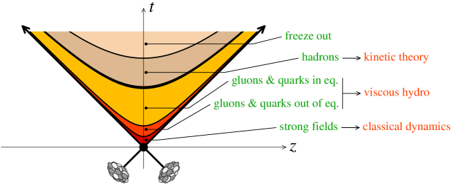
Figure 1: Successive stages of a heavy ion collision.

An effective way of describing the physics of gluon saturation and calculating QCD processes in this regime came a bit later, firstly in the form of the McLerran-Venugopalan model McLerran:1994ni where the degrees of freedom were identified and the classical aspects of their dynamics recognized. In this model, the degrees of freedom with a large longitudinal momentum (in the observer’s frame) contribute via the color flow they carry, and are treated as static variables thanks to Lorentz time dilation (the internal dynamics of a hadron appears frozen in the observer’s frame, on the timescale of the collision). This simplification does not apply to gluons in the vicinity of the observer’s rapidity, and they are treated as conventional gauge field operators.

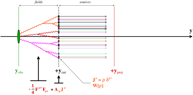
Figure 2: Degrees of freedom in the CGC and their interplay.

In the MV model, the distribution of color sources in the wavefunction of a high energy nucleus was argued to be Gaussian. A few years later, it was realized that this distribution must depend on a longitudinal momentum scale, due to large logarithms coming from loop corrections. This led to the Color Glass Condensate (CGC) effective theory, and to the JIMWLK evolution equation for the distribution of sources Gelis:2010nm .

2 Evolution towards hydrodynamics in the CGC

The CGC provides a tool for systematically calculating observable quantities in heavy ion collisions, such as the gluon spectrum, the energy-momentum tensor, etc… One may think of using the energy-momentum tensor calculated in the CGC framework as an initial condition for hydrodynamical models of the expansion of the fireball produced in heavy ion collisions. Such a matching is justified theoretically provided that the two descriptions (CGC and hydrodynamics) agree over some non-empty time range.

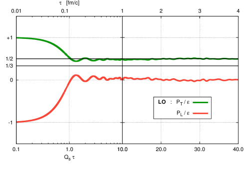
Figure 3: Ratio of the transverse and longitudinal pressures to the energy density in the CGC at leading order. The lower times axis is in units of $1/Q_{s}$. The upper axis gives absolute values for the specific choice $Q_{s}=2\leavevmode\nobreak\$GeV.

At leading order, the CGC leads to a very simple answer, since all inclusive observables can be expressed in terms of a classical solution of the Yang-Mills equations. However, this classical approximation leads to an energy-momentum tensor whose behavior is difficult to reconcile with hydrodynamics. Just after the collision, the longitudinal pressure is negative. It increases and becomes mostly positive at a time $Q_{s}\tau\sim 1$. However, the ratio of longitudinal to transverse pressure decreases forever, while it increases in hydrodynamics.

In higher orders, the energy-momentum tensor receives quantum contributions, beyond that of the LO classical fields. Despite being suppressed by a power of $\alpha_{s}$, these corrections may be large because of instabilities that exist in classical solutions of Yang-Mills equations. Indeed, NLO corrections can be expressed in terms of perturbations around the LO classical solutions, that grow exponentially in the presence of unstable modes.

Thus, instead of a strict NLO calculation, one should seek for a resummation. One such framework is provided by the classical statistical approximation (CSA), in which one performs an average over classical solutions obtained from Gaussian fluctuating initial conditions. In the limit where the variance of the fluctuations goes to zero, one recovers a unique classical evolution. Several implementations of this scheme have been proposed in the literature, that differ in the distribution of fluctuating initial fields.

1. There exists an ensemble of initial fields such that the CSA contains the leading and next-to-leading orders exactly Epelbaum:2013waa ; Gelis:2013rba , and a subset of all higher orders. In order to achieve this, the initial fields must be the sum of the leading order classical field ${\cal A}^{\mu a}(x)$ (non fluctuating) and a linear superposition of mode functions $a^{\mu a}_{{\boldsymbol{k}}\lambda c}(x)$:

$$A^{\mu a}(x)={\cal A}^{\mu a}(x)+\sum_{\lambda,c}\int_{\boldsymbol{k}}\frac{d^{3}{\boldsymbol{k}}}{(2\pi)^{3}2|{\boldsymbol{k}}|}\;\Big{[}c_{{\boldsymbol{k}}\lambda c}\,a^{\mu a}_{{\boldsymbol{k}}\lambda c}(x)+\mbox{c.c.}\Big{]}\;,$$

$$\big{<}c_{{\boldsymbol{k}}\lambda c}\big{>}=0\;,\quad\big{<}c_{{\boldsymbol{k}}\lambda c}^{\ }c_{{\boldsymbol{k}}^{\prime}\lambda^{\prime}c^{\prime}}^{*}\big{>}=\frac{1}{2}\;2\big{|}{\boldsymbol{k}}\big{|}\,(2\pi)^{3}\delta({\boldsymbol{k}}-{\boldsymbol{k}}^{\prime})\,\delta_{\lambda\lambda^{\prime}}\,\delta_{cc^{\prime}}\;.$$ (1)

In this formula, the functions $a^{\mu a}_{{\boldsymbol{k}}\lambda c}(x)$ are solutions of the Yang-Mills equations linearized about the field ${\cal A}^{\mu a}$; with plane wave initial conditions (of momentum ${\boldsymbol{k}}$, polarization $\lambda$ and color $c$). The coefficients $c_{{\boldsymbol{k}}\lambda c}$ are random Gaussian distributed, with a null mean value and the variance given in the second line. The prefactor $1/2$ in this variance can be interpreted as the occupation number corresponding to the quantum fluctuations in each quantum mode. Since this setup reproduces the one loop result, it also leads to the usual one-loop ultraviolet divergences. In addition, it also contains extra ultraviolet divergences that do not exist in the underlying theory. These spurious divergences originate from the fact that the CSA is a non-renormalizable scheme: starting at two loops, it contains divergences that cannot be removed by a renormalization of the parameters of the Lagrangian Epelbaum:2014yja . This leads to a very strong dependence on the ultraviolet cutoff when it is chosen much larger than the physical scales Berges:2013lsa ; Epelbaum:2014mfa .

2. Another implementation of the CSA uses as initial condition fluctuating fields that correspond to a gas of gluons with a distribution $f({\boldsymbol{k}})$. These initial fields have no non-fluctuating part, and the variance of the random coefficients is proportional to $f({\boldsymbol{k}})$ Berges:2013eia ; Berges:2013fga ; Berges:2014bba :

$$A^{\mu a}(x)=\sum_{\lambda,c}\int_{\boldsymbol{k}}\frac{d^{3}{\boldsymbol{k}}}{(2\pi)^{3}2|{\boldsymbol{k}}|}\;\Big{[}c_{{\boldsymbol{k}}\lambda c}\,a^{\mu a}_{{\boldsymbol{k}}\lambda c}(x)+\mbox{c.c.}\Big{]}\;,$$

$$\big{<}c_{{\boldsymbol{k}}\lambda c}\big{>}=0\;,\quad\big{<}c_{{\boldsymbol{k}}\lambda c}^{\ }c_{{\boldsymbol{k}}^{\prime}\lambda^{\prime}c^{\prime}}^{*}\big{>}=f({\boldsymbol{k}})\;2\big{|}{\boldsymbol{k}}\big{|}\,(2\pi)^{3}\delta({\boldsymbol{k}}-{\boldsymbol{k}}^{\prime})\,\delta_{\lambda\lambda^{\prime}}\,\delta_{cc^{\prime}}\;.$$ (2)

(Note the fact that in eq. (2) the distribution $f({\boldsymbol{k}})$ replaces the $1/2$ of eq. (1).) This implementation of the CSA leads to ultraviolet finite results provided that the distribution $f({\boldsymbol{k}})$ decreases sufficiently fast, but it does not contain any quantum fluctuations.

Eqs. (1) and (2) describe rather different situations, despite their resemblance: the flat spectrum of Eq. (1) on top of a non-fluctuating classical field describes a quantum coherent state, while the spectrum of Eq. (2), with compact support, describes an incoherent classical state. When applied to simulations of the early stages of heavy ion collisions, these two types of fluctuating initial conditions lead to quite different behaviors of the pressure tensor. The setup 1 leads to a roughly constant ratio $P_{{}_{L}}/P_{{}_{T}}$ on short timescales, of the order of a few $Q_{s}^{-1}$, while the setup 2 leads to a ratio $P_{{}_{L}}/P_{{}_{T}}$ that decreases forever. Based on the time evolution of the particle distribution in the second setup, it has been argued that quantum corrections may be ignored up to large times of order $\alpha_{s}^{-3/2}Q_{s}^{-1}$.

3 Kinetic theory approach

To clarify the role of quantum fluctuations in the process of isotropization, one should include them while preserving renormalizability. A field theoretic framework that does this is the 2-particle irreducible approximation Luttinger:1960ua ; Aarts:2002dj ; Calzetta:2002ub ; Berges:2004pu of the Kadanoff-Baym equations. Although in principle applicable to a longitudinally expanding system Hatta:2011ky ; Hatta:2012gq , this still remains a challenging task. A computationally much cheaper alternative is to use kinetic theory Epelbaum:2014mfa in order to investigate the role of quantum fluctuations. Indeed, the implementations 1 and 2 of the CSA described in the previous section correspond to definite Feynman rules in which certain vertices are omitted and where a propagator is approximated. By using these truncated Feynman rules in the calculation of the appropriate self-energy diagrams, one can obtain the kinetic analogue of the approximations 1 and 2. The Boltzmann equation with $2\to 2$ scatterings reads:

$$\partial_{t}f_{3} \sim g^{4}\int_{124}\cdots\big{[}f_{1}f_{2}({f_{3}+f_{4}})-{f_{3}f_{4}}(f_{1}+f_{2})\big{]}$$ (3)

$$\quad+g^{4}\int_{124}\cdots\big{[}f_{1}f_{2}-{f_{3}f_{4}}\big{]}\;.$$

where the dots contain the cross-section and the delta functions for the conservation of energy and momentum. In Eq. (3), the first line contains the terms that remain in the classical approximation of Eq. (2) (see refs. Mueller:2002gd ; Jeon:2004dh ), and the terms on the second line come from quantum fluctuations. Ignoring these terms quadratic in the distribution $f$ is the kinetic theory analogue of the implementation 2 of the CSA.

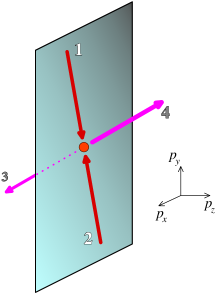
Figure 4: Kinematics of a $2\to 2$ scattering process that would contribute to the isotropization of pressures when the particle distribution is very anisotropic (with $p_{z}\approx 0$). The momenta of the two particles in the initial state are purely transverse, and the outgoing particles have opposite $p_{z}$’s.

The cubic terms of the first line are dominant in the regime of large occupation number. But since this approximation is usually not uniform across all momentum space, this may lead to problems especially when the distribution is very anisotropic. In Fig. 4, we illustrate this for such a distribution, for which the incoming particles 1,2 have almost purely transverse momenta. Isotropization would require that one of the outgoing particles (3 or 4) has a nonzero $p_{z}$. With this kinematics, non vanishing contributions can only come from the second line, which is neglected in the classical approximation.

This has been seen in numerical studies of the Boltzmann equation for a longitudinally expanding system, both for scalar fields Epelbaum:2015vxa and for gluons Kurkela:2015qoa , with CGC-like highly occupied initial distributions of the form $f_{0}({\boldsymbol{k}})=(n_{0}/g^{2})\,\theta(Q_{s}-k_{\perp})\,\theta(\xi Q_{s}-|k_{z}|)$ at a time of order $Q_{s}^{-1}$. When one keeps only the classical terms, the Boltzmann equation leads to a forever decreasing $P_{{}_{L}}/P_{{}_{T}}$ (see Fig. 5, and the curve $\lambda=0$ in Fig. 7). Moreover, like in the setup 2 of the CSA, the classical approximation of the Boltzmann equation leads to a classical attractor: the asymptotic behavior of these classical evolutions is universal, regardless of the details of the initial condition.

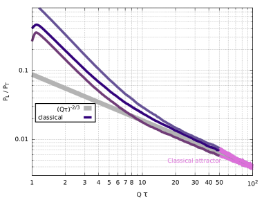
Figure 5: Time evolution of the ratio $P_{{}_{L}}/P_{{}_{T}}$ in the classical approximation of the Boltzmann equation. When the initial condition is of the form $f_{0}({\boldsymbol{p}})=(n_{0}/g^{2}){\bf f}({\boldsymbol{p}})$, the classical evolution does not depend on the coupling and its value need not be specified. The three curves correspond to various CGC-like initial conditions that differ in the magnitude of the initial anisotropy. All these evolutions converge towards a universal classical attractor.

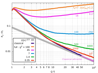
Figure 6: Time evolution of the ratio $P_{{}_{L}}/P_{{}_{T}}$ obtained from the full Boltzmann equation, for various values of the coupling constant. The initial condition is of the form $f_{0}({\boldsymbol{p}})=(n_{0}/g^{2}){\bf f}({\boldsymbol{p}})$. The evolution in the classical approximation is shown for the same initial condition for comparison. The numbers $f_{0}$ and $[\eta/s]_{\rm eq}$ overlaid on the plot indicate the corresponding initial occupation number and the equilibrium value of the viscosity to entropy ratio (in equilibrium).

The figure 6 (for scalar fields) and the curves labeled $\lambda=0.5$ to $10$ in Fig. 4 (for gluons in Yang-Mills theory) show the results obtained with the full Boltzmann equation, including the terms of quantum origin (the second line in eq. (3)). These results show that it takes very small couplings (or equivalently, very large values of the ratio $\eta/s$) and very large occupation numbers for the quantum evolution to get close to the universal classical behavior. For larger yet still small couplings, the classical and quantum evolutions depart from each other very early: for instance, in the Yang-Mills case at $\lambda=0.5$ (i.e. $\alpha_{s}\approx 0.02$ for $N_{c}=2$ colors), this happens around $Q_{s}\tau\approx 2$, well before the conjectured limit of validity of the classical approximation, $Q_{s}\tau\approx\alpha_{s}^{-3/2}\approx 350$. This indicates that quantum fluctuations are essential for isotropization: purely classical approximations do not correctly capture the relevant physics and largely overestimate their own range of validity.

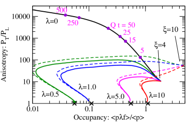
Figure 7: Evolution of the anisotropy and momentum weighted occupation number in a system of gluons described in kinetic theory, for initial conditions of the form $f_{0}({\boldsymbol{p}})=(n_{0}/\lambda){\bf f}({\boldsymbol{p}})$. The curve labeled $\lambda=0$ is a classical approximation, while the curves for $\lambda=0.5,1,5,10$ are obtained with the full Boltzmann equation. Plot taken from Kurkela:2015qoa , with time labels added by us for clarity.

References

- (1) L.D. McLerran, R. Venugopalan, Phys. Rev. D49, 2233 (1994)
- (2) F. Gelis, E. Iancu, J. Jalilian-Marian, R. Venugopalan, Ann. Rev. Nucl. Part. Sci. 60, 463 (2010), 1002.0333
- (3) T. Epelbaum, F. Gelis, Phys. Rev. D88, 085015 (2013), 1307.1765
- (4) T. Epelbaum, F. Gelis, Phys. Rev. Lett. 111, 232301 (2013), 1307.2214
- (5) T. Epelbaum, F. Gelis, B. Wu, Phys. Rev. D90, 065029 (2014), 1402.0115
- (6) J. Berges, K. Boguslavski, S. Schlichting, R. Venugopalan, JHEP 05, 054 (2014), 1312.5216
- (7) J. Berges, K. Boguslavski, S. Schlichting, R. Venugopalan, Phys. Rev. D89, 074011 (2014), 1303.5650
- (8) J. Berges, K. Boguslavski, S. Schlichting, R. Venugopalan, Phys. Rev. D89, 114007 (2014), 1311.3005
- (9) J. Berges, K. Boguslavski, S. Schlichting, R. Venugopalan, Phys. Rev. Lett. 114, 061601 (2015), 1408.1670
- (10) J.M. Luttinger, J.C. Ward, Phys. Rev. 118, 1417 (1960)
- (11) G. Aarts, D. Ahrensmeier, R. Baier, J. Berges, J. Serreau, Phys. Rev. D66, 045008 (2002), hep-ph/0201308
- (12) E.A. Calzetta, B.L. Hu (2002), hep-ph/0205271
- (13) J. Berges, Phys. Rev. D70, 105010 (2004), hep-ph/0401172
- (14) Y. Hatta, A. Nishiyama, Nucl. Phys. A873, 47 (2012), 1108.0818
- (15) Y. Hatta, A. Nishiyama, Phys. Rev. D86, 076002 (2012), 1206.4743
- (16) T. Epelbaum, F. Gelis, N. Tanji, B. Wu, Phys. Rev. D90, 125032 (2014), 1409.0701
- (17) A.H. Mueller, D.T. Son, Phys. Lett. B582, 279 (2004), hep-ph/0212198
- (18) S. Jeon, Phys. Rev. C72, 014907 (2005), hep-ph/0412121
- (19) T. Epelbaum, F. Gelis, S. Jeon, G. Moore, B. Wu, JHEP 09, 117 (2015), 1506.05580
- (20) A. Kurkela, Y. Zhu, Phys. Rev. Lett. 115, 182301 (2015), 1506.06647