The Eddy Current–LLG Equations–Part I: FEM-BEM Coupling

Abstract.

We analyse a numerical method for the coupled system of the eddy current equations in ${\mathbb{R}}^{3}$ with the Landau-Lifshitz-Gilbert equation in a bounded domain. The unbounded domain is discretised by means of finite-element/boundary-element coupling. Even though the considered problem is strongly nonlinear, the numerical approach is constructed such that only two linear systems per time step have to be solved. In this first part of the paper, we prove unconditional weak convergence (of a subsequence) of the finite-element solutions towards a weak solution. A priori error estimates will be presented in the second part.

1. Introduction

This paper deals with the coupling of finite element and boundary element methods to solve the system of the eddy current equations in the whole 3D spatial space and the Landau-Lifshitz-Gilbert equation (LLG), the so-called ELLG system or equations. The system is also called the quasi-static Maxwell-LLG (MLLG) system.

The LLG is widely considered as a valid model of micromagnetic phenomena occurring in, e.g., magnetic sensors, recording heads, and magneto-resistive storage device [21, 23, 29]. Classical results concerning existence and non-uniqueness of solutions can be found in [5, 31]. In a ferro-magnetic material, magnetisation is created or affected by external electro-magnetic fields. It is therefore necessary to augment the Maxwell system with the LLG, which describes the influence of ferromagnet; see e.g. [18, 22, 31]. Existence, regularity and local uniqueness for the MLLG equations are studied in [17].

Throughout the literature, there are various works on numerical approximation methods for the LLG, ELLG, and MLLG equations [3, 4, 10, 11, 18, 24, 25] (the list is not exhausted), and even with the full Maxwell system on bounded domains [7, 8], and in the whole ${\mathbb{R}}^{3}$ [16]. Originating from the seminal work [3], the recent works [24, 25] consider a similar numeric integrator for a bounded domain.

This work studies the ELLG equations where we consider the electromagnetic field on the whole ${\mathbb{R}}^{3}$ and do not need to introduce artificial boundaries. Differently from [16] where the Faedo-Galerkin method is used to prove existence of weak solutions, we extend the analysis for the integrator used in [3, 24, 25] to a finite-element/boundary-element (FEM/BEM) discretisation of the eddy current part on ${\mathbb{R}}^{3}$. This is inspired by the FEM/BEM coupling approach designed for the pure eddy current problem in [13], which allows to treat unbounded domains without introducing artificial boundaries. Two approaches are proposed in [13]: the so-called “magnetic (or $\boldsymbol{H}$-based) approach” which eliminates the electric field, retaining only the magnetic field as the unknown in the system, and the “electric (or $\boldsymbol{E}$-based) approach” which considers a primitive of the electric field as the only unknown. The coupling of the eddy-current system with the LLG dictates that the first approach is more appropriate; see (2.1).

The main result of this first part is the weak convergence of the discrete approximation towards a weak solution without any condition on the space and time discretisation. This also proves the existence of weak solutions.

The remainder of this part is organised as follows. Section 2 introduces the coupled problem and the notation, presents the numerical algorithm, and states the main result of this part of the paper. Section 3 is devoted to the proof of this main result. Numerical results are presented in Section 4. The second part of this paper [20] proves a priori estimates for the proposed algorithm.

2. Model Problem & Main Result

2.1. The problem

Consider a bounded Lipschitz domain $D\subset{\mathbb{R}}^{3}$ with connected boundary $\Gamma$ having the outward normal vector $\boldsymbol{n}$. We define $D^{\ast}:={\mathbb{R}}^{3}\setminus\overline{D}$, $D_{T}:=(0,T)\times D$, $\Gamma_{T}:=(0,T)\times\Gamma$, $D_{T}^{\ast}:=(0,T)\times D^{\ast}$, and ${\mathbb{R}}^{3}_{T}:=(0,T)\times{\mathbb{R}}^{3}$ for $T>0$. We start with the quasi-static approximation of the full Maxwell-LLG system from [31] which reads as

$$\boldsymbol{m}_{t}-\alpha\boldsymbol{m}\times\boldsymbol{m}_{t} =-\boldsymbol{m}\times\boldsymbol{H}_{\rm eff} \quad\text{in }D_{T},$$ (2.1a)

$$\sigma\boldsymbol{E}-\nabla\times\boldsymbol{H} =0 \quad\text{in }{\mathbb{R}}^{3}_{T},$$ (2.1b)

$$\mu_{0}\boldsymbol{H}_{t}+\nabla\times\boldsymbol{E} =-\mu_{0}\widetilde{\boldsymbol{m}}_{t} \quad\text{in }{\mathbb{R}}^{3}_{T},$$ (2.1c)

$${\rm div}(\boldsymbol{H}+\widetilde{\boldsymbol{m}}) =0 \quad\text{in }{\mathbb{R}}^{3}_{T},$$ (2.1d)

$${\rm div}(\boldsymbol{E}) =0 \quad\text{in }D^{\ast}_{T},$$ (2.1e)

where $\widetilde{\boldsymbol{m}}$ is the zero extension of $\boldsymbol{m}$ to ${\mathbb{R}}^{3}$ and $\boldsymbol{H}_{\rm eff}$ is the effective field defined by $\boldsymbol{H}_{\rm eff}=C_{e}\Delta\boldsymbol{m}+\boldsymbol{H}$ for some constant $C_{e}>0$. Here the parameter $\alpha>0$ and permability $\mu_{0}\geq 0$ are constants, whereas the conductivity $\sigma$ takes a constant positive value in $D$ and the zero value in $D^{\ast}$. Equation (2.1d) is understood in the distributional sense because there is a jump of $\widetilde{\boldsymbol{m}}$ across $\Gamma$.

It follows from (2.1a) that $|\boldsymbol{m}|$ is constant. We follow the usual practice to normalise $|\boldsymbol{m}|$ (and thus the same condition is required for $|\boldsymbol{m}^{0}|$). The following conditions are imposed on the solutions of (2.1):

$$\partial_{n}\boldsymbol{m} =0 \quad\text{on }\Gamma_{T},$$ (2.2a)

$$|\boldsymbol{m}| =1 \quad\text{in }D_{T},$$ (2.2b)

$$\boldsymbol{m}(0,\cdot) =\boldsymbol{m}^{0} \quad\text{in }D,$$ (2.2c)

$$\boldsymbol{H}(0,\cdot) =\boldsymbol{H}^{0} \quad\text{in }{\mathbb{R}}^{3},$$ (2.2d)

$$\boldsymbol{E}(0,\cdot) =\boldsymbol{E}^{0} \quad\text{in }{\mathbb{R}}^{3},$$ (2.2e)

$$|\boldsymbol{H}(t,x)| =\mathcal{O}(|x|^{-1}) \quad\text{as }|x|\to\infty,$$ (2.2f)

where $\partial_{n}$ denotes the normal derivative. The initial data $\boldsymbol{m}^{0}$ and $\boldsymbol{H}^{0}$ satisfy $|\boldsymbol{m}^{0}|=1$ in $D$ and

$$\begin{split}{\rm div}(\boldsymbol{H}^{0}+\widetilde{\boldsymbol{m}}^{0})&=0\quad\text{in }{\mathbb{R}}^{3}.\end{split}$$ (2.3)

Below, we focus on an $\boldsymbol{H}$-based formulation of the problem. It is possible to recover $\boldsymbol{E}$ once $\boldsymbol{H}$ and $\boldsymbol{m}$ are known; see (2.12)

2.2. Function spaces and notations

Before introducing the concept of weak solutions to problem (2.1)–(2.2) we need the following definitions of function spaces. Let ${\mathbb{L}}^{2}{(D}):=L^{2}(D;{\mathbb{R}}^{3})$ and ${\mathbb{H}}({\rm curl},D):=\big{\{}\boldsymbol{w}\in{\mathbb{L}}^{2}{(D})\,:\,\nabla\times\boldsymbol{w}\in{\mathbb{L}}^{2}{(D})\big{\}}$. We define $H^{1/2}(\Gamma)$ as the usual trace space of $H^{1}(D)$ and define its dual space $H^{-1/2}(\Gamma)$ by extending the $L^{2}$-inner product on $\Gamma$. For convenience we denote

$${\mathcal{X}}:=\big{\{}(\boldsymbol{\xi},\zeta)\in{\mathbb{H}}({\rm curl},D)\times H^{1/2}(\Gamma)\,:\,\boldsymbol{n}\times\boldsymbol{\xi}|_{\Gamma}=\boldsymbol{n}\times\nabla_{\Gamma}\zeta\text{ in the sense of traces}\big{\}}.$$

Recall that $\boldsymbol{n}\times\boldsymbol{\xi}|_{\Gamma}$ is the tangential trace (or twisted tangential trace) of $\boldsymbol{\xi}$, and $\nabla_{\Gamma}\zeta$ is the surface gradient of $\zeta$. Their definitions and properties can be found in [14, 15].

Finally, if $X$ is a normed vector space then $L^{2}(0,T;X)$, $H^{m}(0,T;X)$, and $W^{m,p}(0,T;X)$ denote the usual corresponding Lebesgues and Sobolev spaces of functions defined on $(0,T)$ and taking values in $X$.

We finish this subsection with the clarification of the meaning of the cross product between different mathematical objects. For any vector functions $\boldsymbol{u},\boldsymbol{v},\boldsymbol{w}$ we denote

$$\boldsymbol{u}\times\nabla\boldsymbol{v}:=\left(\boldsymbol{u}\times\frac{\partial\boldsymbol{v}}{\partial x_{1}},\boldsymbol{u}\times\frac{\partial\boldsymbol{v}}{\partial x_{2}},\boldsymbol{u}\times\frac{\partial\boldsymbol{v}}{\partial x_{3}}\right),\quad\nabla\boldsymbol{u}\times\nabla\boldsymbol{v}:=\sum_{i=1}^{3}\frac{\partial\boldsymbol{u}}{\partial x_{i}}\times\frac{\partial\boldsymbol{v}}{\partial x_{i}}$$

and

$$(\boldsymbol{u}\times\nabla\boldsymbol{v})\cdot\nabla\boldsymbol{w}:=\sum_{i=1}^{3}\left(\boldsymbol{u}\times\frac{\partial\boldsymbol{v}}{\partial x_{i}}\right)\cdot\frac{\partial\boldsymbol{w}}{\partial x_{i}}.$$

2.3. Weak solutions

A weak formulation for (2.1a) is well-known, see e.g. [3, 25]. Indeed, by multiplying (2.1a) by $\boldsymbol{\phi}\in C^{\infty}(D_{T};{\mathbb{R}}^{3})$, using $|\boldsymbol{m}|=1$ and integration by parts, we deduce

$$\alpha\langle\boldsymbol{m}_{t}\,,\,\boldsymbol{m}\times\boldsymbol{\phi}\rangle_{D_{T}}+\langle\boldsymbol{m}\times\boldsymbol{m}_{t}\,,\,\boldsymbol{m}\times\boldsymbol{\phi}\rangle_{D_{T}}+C_{e}\langle\nabla\boldsymbol{m}\,,\,\nabla(\boldsymbol{m}\times\boldsymbol{\phi})\rangle_{D_{T}}=\langle\boldsymbol{H}\,,\,\boldsymbol{m}\times\boldsymbol{\phi}\rangle_{D_{T}}.$$

To tackle the eddy current equations on ${\mathbb{R}}^{3}$, we aim to employ FE/BE coupling methods. To that end, we employ the magnetic approach from [13], which eventually results in a variant of the Trifou-discretisation of the eddy-current Maxwell equations. The magnetic approach is more or less mandatory in our case, since the coupling with the LLG equation requires the magnetic field rather than the electric field.

Multiplying (2.1c) by $\boldsymbol{\xi}\in C^{\infty}(D,{\mathbb{R}}^{3})$ satisfying $\nabla\times\boldsymbol{\xi}=0$ in $D^{\ast}$, integrating over ${\mathbb{R}}^{3}$, and using integration by parts, we obtain for almost all $t\in[0,T]$

$$\mu_{0}\langle\boldsymbol{H}_{t}(t)\,,\,\boldsymbol{\xi}\rangle_{{\mathbb{R}}^{3}}+\langle\boldsymbol{E}(t)\,,\,\nabla\times\boldsymbol{\xi}\rangle_{{\mathbb{R}}^{3}}=-\mu_{0}\langle\boldsymbol{m}_{t}(t)\,,\,\boldsymbol{\xi}\rangle_{D}.$$

Using $\nabla\times\boldsymbol{\xi}=0$ in $D^{\ast}$ and (2.1b) we deduce

$$\mu_{0}\langle\boldsymbol{H}_{t}(t)\,,\,\boldsymbol{\xi}\rangle_{{\mathbb{R}}^{3}}+\sigma^{-1}\langle\nabla\times\boldsymbol{H}(t)\,,\,\nabla\times\boldsymbol{\xi}\rangle_{D}=-\mu_{0}\langle\boldsymbol{m}_{t}(t)\,,\,\boldsymbol{\xi}\rangle_{D}.$$

Since $\nabla\times\boldsymbol{H}=\nabla\times\boldsymbol{\xi}=0$ in $D^{\ast}$, there exists $\varphi$ and $\zeta$ such that $\boldsymbol{H}=\nabla\varphi$ and $\boldsymbol{\xi}=\nabla\zeta$ in $D^{\ast}$. Therefore, the above equation can be rewritten as

$$\mu_{0}\langle\boldsymbol{H}_{t}(t)\,,\,\boldsymbol{\xi}\rangle_{D}+\mu_{0}\langle\nabla\varphi_{t}(t)\,,\,\nabla\zeta\rangle_{D^{\ast}}+\sigma^{-1}\langle\nabla\times\boldsymbol{H}(t)\,,\,\nabla\times\boldsymbol{\xi}\rangle_{D}=-\mu_{0}\langle\boldsymbol{m}_{t}(t)\,,\,\boldsymbol{\xi}\rangle_{D}.$$

Since (2.1d) implies ${\rm div}(\boldsymbol{H})=0$ in $D^{\ast}$, we have $\Delta\varphi=0$ in $D^{\ast}$, so that (formally) $\Delta\varphi_{t}=0$ in $D^{\ast}$. Hence integration by parts yields

$$\mu_{0}\langle\boldsymbol{H}_{t}(t)\,,\,\boldsymbol{\xi}\rangle_{D}-\mu_{0}\langle\partial_{n}^{+}\varphi_{t}(t)\,,\,\zeta\rangle_{\Gamma}+\sigma^{-1}\langle\nabla\times\boldsymbol{H}(t)\,,\,\nabla\times\boldsymbol{\xi}\rangle_{D}=-\mu_{0}\langle\boldsymbol{m}_{t}(t)\,,\,\boldsymbol{\xi}\rangle_{D},$$ (2.4)

where $\partial_{n}^{+}$ is the exterior Neumann trace operator with the limit taken from $D^{\ast}$. The advantage of the above formulation is that no integration over the unbounded domain $D^{\ast}$ is required. The exterior Neumann trace $\partial_{n}^{+}\varphi_{t}$ can be computed from the exterior Dirichlet trace $\lambda$ of $\varphi$ by using the Dirichlet-to-Neumann operator $\mathfrak{S}$, which is defined as follows.

Let $\gamma^{-}$ be the interior Dirichlet trace operator and $\partial_{n}^{-}$ be the interior normal derivative or Neumann trace operator. (The $-$ sign indicates the trace is taken from $D$.) Recalling the fundamental solution of the Laplacian $G(x,y):=1/(4\pi|x-y|)$, we introduce the following integral operators defined formally on $\Gamma$ as

$$\mathfrak{V}(\lambda):=\gamma^{-}\overline{\mathfrak{V}}(\lambda),\quad\mathfrak{K}(\lambda):=\gamma^{-}\overline{\mathfrak{K}}(\lambda)+\mbox{$\frac{1}{2}$},\quad\text{and}\quad\mathfrak{W}(\lambda):=-\partial_{n}^{-}\overline{\mathfrak{K}}(\lambda),$$

where, for $x\notin\Gamma$,

$$\overline{\mathfrak{V}}(\lambda)(x):=\int_{\Gamma}G(x,y)\lambda(y)\,ds_{y}\quad\text{and}\quad\overline{\mathfrak{K}}(\lambda)(x):=\int_{\Gamma}\partial_{n(y)}G(x,y)\lambda(y)\,ds_{y}.$$

Moreover, let $\mathfrak{K}^{\prime}$ denote the adjoint operator of $\mathfrak{K}$ with respect to the extended $L^{2}$-inner product. Then the exterior Dirichlet-to-Neumann map $\mathfrak{S}\colon H^{1/2}(\Gamma)\to H^{-1/2}(\Gamma)$ can be represented as

$$\mathfrak{S}=-\mathfrak{V}^{-1}(1/2-\mathfrak{K}).$$ (2.5)

Another more symmetric representation is

$$\mathfrak{S}=-(1/2-\mathfrak{K}^{\prime})\mathfrak{V}^{-1}(1/2-\mathfrak{K})-\mathfrak{W}.$$ (2.6)

Recall that $\varphi$ satisfies $\boldsymbol{H}=\nabla\varphi$ in $D^{\ast}$. We can choose $\varphi$ satisfying $\varphi(x)=O(|x|^{-1})$ as $|x|\to\infty$. Now if $\lambda=\gamma^{+}\varphi$ then $\lambda_{t}=\gamma^{+}\varphi_{t}$. Since $\Delta\varphi=\Delta\varphi_{t}=0$ in $D^{\ast}$, and since the exterior Laplace problem has a unique solution we have $\mathfrak{S}\lambda=\partial_{n}^{+}\varphi$ and $\mathfrak{S}\lambda_{t}=\partial_{n}^{+}\varphi_{t}$. Hence (2.4) can be rewritten as

$$\langle\boldsymbol{H}_{t}(t)\,,\,\boldsymbol{\xi}\rangle_{D}-\langle\mathfrak{S}\lambda_{t}(t)\,,\,\zeta\rangle_{\Gamma}+\mu_{0}^{-1}\sigma^{-1}\langle\nabla\times\boldsymbol{H}(t)\,,\,\nabla\times\boldsymbol{\xi}\rangle_{D}=-\langle\boldsymbol{m}_{t}(t)\,,\,\boldsymbol{\xi}\rangle_{D}.$$ (2.7)

We remark that if $\nabla_{\Gamma}$ denotes the surface gradient operator on $\Gamma$ then it is well-known that $\nabla_{\Gamma}\lambda=(\nabla\varphi)|_{\Gamma}-(\partial_{n}^{+}\varphi)\boldsymbol{n}=\boldsymbol{H}|_{\Gamma}-(\partial_{n}^{+}\varphi)\boldsymbol{n};$ see e.g. [28, Section 3.4]. Hence $\boldsymbol{n}\times\nabla_{\Gamma}\lambda=\boldsymbol{n}\times\boldsymbol{H}|_{\Gamma}$.

The above analysis prompts us to define the following weak formulation.

Definition 1.

A triple $(\boldsymbol{m},\boldsymbol{H},\lambda)$ satisfying

$$\boldsymbol{m} \in{\mathbb{H}}^{1}{(D_{T}})\quad\text{and}\quad\boldsymbol{m}_{t}|_{\Gamma_{T}}\in L^{2}(0,T;H^{-1/2}(\Gamma)),$$

$$\boldsymbol{H} \in L^{2}(0,T;{\mathbb{H}}({\rm curl},D))\cap H^{1}(0,T;{\mathbb{L}}^{2}{(D})),$$

$$\lambda \in H^{1}(0,T;H^{1/2}(\Gamma))$$

is called a weak solution to (2.1)–(2.2) if the following statements hold

1. $|\boldsymbol{m}|=1$ almost everywhere in $D_{T}$;

2. $\boldsymbol{m}(0,\cdot)=\boldsymbol{m}^{0}$, $\boldsymbol{H}(0,\cdot)=\boldsymbol{H}^{0}$, and $\lambda(0,\cdot)=\gamma^{+}\varphi^{0}$ where $\varphi^{0}$ is a scalar function satisfies $\boldsymbol{H}^{0}=\nabla\varphi^{0}$ in $D^{\ast}$ (the assumption (2.3) ensures the existence of $\varphi^{0}$);

3. For all $\boldsymbol{\phi}\in C^{\infty}(D_{T};{\mathbb{R}}^{3})$

   $$\alpha\langle\boldsymbol{m}_{t}\,,\,\boldsymbol{m}\times\boldsymbol{\phi}\rangle_{D_{T}} +\langle\boldsymbol{m}\times\boldsymbol{m}_{t}\,,\,\boldsymbol{m}\times\boldsymbol{\phi}\rangle_{D_{T}}+C_{e}\langle\nabla\boldsymbol{m}\,,\,\nabla(\boldsymbol{m}\times\boldsymbol{\phi})\rangle_{D_{T}}$$

   $$=\langle\boldsymbol{H}\,,\,\boldsymbol{m}\times\boldsymbol{\phi}\rangle_{D_{T}};$$ (2.8a)

4. There holds $\boldsymbol{n}\times\nabla_{\Gamma}\lambda=\boldsymbol{n}\times\boldsymbol{H}|_{\Gamma}$ in the sense of traces;

5. For $\boldsymbol{\xi}\in C^{\infty}(D;{\mathbb{R}}^{3})$ and $\zeta\in C^{\infty}(\Gamma)$ satisfying $\boldsymbol{n}\times\boldsymbol{\xi}|_{\Gamma}=\boldsymbol{n}\times\nabla_{\Gamma}\zeta$ in the sense of traces

   $$\langle\boldsymbol{H}_{t}\,,\,\boldsymbol{\xi}\rangle_{D_{T}}-\langle\mathfrak{S}\lambda_{t}\,,\,\zeta\rangle_{\Gamma_{T}}+\sigma^{-1}\mu_{0}^{-1}\langle\nabla\times\boldsymbol{H}\,,\,\nabla\times\boldsymbol{\xi}\rangle_{D_{T}} =-\langle\boldsymbol{m}_{t}\,,\,\boldsymbol{\xi}\rangle_{D_{T}};$$ (2.8b)

6. For almost all $t\in[0,T]$

   $$\|\nabla\boldsymbol{m}(t)\|_{{\mathbb{L}}^{2}{(D})}^{2}+\|\boldsymbol{H}(t)\|_{{\mathbb{H}}({\rm curl},D)}^{2}+\|\lambda(t)\|_{H^{1/2}(\Gamma)}^{2}$$

   $$+\|\boldsymbol{m}_{t}\|_{{\mathbb{L}}^{2}{(D_{t}})}^{2}+\|\boldsymbol{H}_{t}\|_{{\mathbb{L}}^{2}{(D_{t}})}^{2}+\|\lambda_{t}\|_{H^{1/2}(\Gamma_{t})}^{2}\leq C,$$ (2.9)

   where the constant $C>0$ is independent of $t$.

The reason we integrate over $[0,T]$ in (2.7) to have (2.8b) is to facilitate the passing to the limit in the proof of the main theorem. The following lemma justifies the above definition.

Lemma 2.

Let $(\boldsymbol{m},\boldsymbol{H},\boldsymbol{E})$ be a strong solution of (2.1)–(2.2). If $\varphi\in H(0,T;H^{1}(D^{\ast}))$ satisfies $\nabla\varphi=\boldsymbol{H}|_{D^{\ast}_{T}}$, and if $\lambda:=\gamma^{+}\varphi$, then the triple $(\boldsymbol{m},\boldsymbol{H}|_{D_{T}},\lambda)$ is a weak solution in the sense of Definition 1.

Conversely, let $(\boldsymbol{m},\boldsymbol{H},\lambda)$ be a sufficiently smooth solution in the sense of Definition 1, and let $\varphi$ be the solution of

$$\Delta\varphi=0\text{ in }D^{\ast},\quad\varphi=\lambda\text{ on }\Gamma,\quad\varphi(x)=O(|x|^{-1})\text{ as }|x|\to\infty.$$ (2.10)

Then $(\boldsymbol{m},\overline{\boldsymbol{H}},\boldsymbol{E})$ is a strong solution to (2.1)–(2.2), where $\overline{\boldsymbol{H}}$ is defined by

$$\overline{\boldsymbol{H}}:=\begin{cases}\boldsymbol{H}&\quad\text{in }D_{T},\\ \nabla\varphi&\quad\text{in }D_{T}^{\ast},\end{cases}$$ (2.11)

and $\boldsymbol{E}$ is reconstructed by letting $\boldsymbol{E}=\sigma^{-1}(\nabla\times\boldsymbol{H})$ in $D_{T}$ and by solving

$$\nabla\times\boldsymbol{E} =-\mu_{0}\overline{\boldsymbol{H}}_{t} \quad\text{in }D_{T}^{\ast},$$ (2.12a)

$${\rm div}(\boldsymbol{E}) =0 \quad\text{in }D_{T}^{\ast},$$ (2.12b)

$$\boldsymbol{n}\times\boldsymbol{E}|_{D_{T}^{\ast}} =\boldsymbol{n}\times\boldsymbol{E}|_{D_{T}} \quad\text{on }\Gamma_{T}.$$ (2.12c)

Proof.

We follow [13]. Assume that $(\boldsymbol{m},\boldsymbol{H},\boldsymbol{E})$ satisfies (2.1)–(2.2). Then clearly Statements (1), (2) and (6) in Definition 1 hold, noting (2.3). Statements (3), (4) and (5) also hold due to the analysis above Definition 1. The converse is also true due to the well-posedness of (2.12) as stated in [13, Equation (15)]. ∎

Remark 3.

The solution $\varphi$ to (2.10) can be represented as $\varphi=(1/2+\mathfrak{K})\lambda-\mathfrak{V}\mathfrak{S}\lambda.$

The next subsection defines the spaces and functions to be used in the approximation of the weak solution the sense of Definition 1.

2.4. Discrete spaces and functions

For time discretisation, we use a uniform partition $0\leq t_{i}\leq T$, $i=0,\ldots,N$ with $t_{i}:=ik$ and $k:=T/N$. The spatial discretisation is determined by a (shape) regular triangulation ${\mathcal{T}}_{h}$ of $D$ into compact tetrahedra $T\in{\mathcal{T}}_{h}$ with diameter $h_{T}/C\leq h\leq Ch_{T}$ for some uniform constant $C>0$. Denoting by ${\mathcal{N}}_{h}$ the set of nodes of ${\mathcal{T}}_{h}$, we define the following spaces

$$\SS^{1}({\mathcal{T}}_{h}) :=\big{\{}\phi_{h}\in C(D)\,:\,\phi_{h}|T\in{\mathcal{P}}^{1}(T)\text{ for all }T\in{\mathcal{T}}_{h}\big{\}},$$

$${\mathcal{K}}_{\boldsymbol{\phi}_{h}} :=\big{\{}\boldsymbol{\psi}_{h}\in\SS^{1}({\mathcal{T}}_{h})^{3}\,:\,\boldsymbol{\psi}_{h}(z)\cdot\boldsymbol{\phi}_{h}(z)=0\text{ for all }z\in{\mathcal{N}}_{h}\big{\}},\quad\boldsymbol{\phi}_{h}\in\SS^{1}({\mathcal{T}}_{h})^{3},$$

where ${\mathcal{P}}^{1}(T)$ is the space of polynomials of degree at most 1 on $T$.

For the discretisation of (2.8b), we employ the space ${\mathcal{N}}{\mathcal{D}}^{1}({\mathcal{T}}_{h})$ of first order Nédélec (edge) elements for $\boldsymbol{H}$ and and the space $\SS^{1}({\mathcal{T}}_{h}|_{\Gamma})$ for $\lambda$. Here ${\mathcal{T}}_{h}|_{\Gamma}$ denotes the restriction of the triangulation to the boundary $\Gamma$. It follows from Statement 4 in Definition 1 that for each $t\in[0,T]$, the pair $(\boldsymbol{H}(t),\lambda(t))\in{\mathcal{X}}$. We approximate the space ${\mathcal{X}}$ by

$${\mathcal{X}}_{h}:=\big{\{}(\boldsymbol{\xi},\zeta)\in{\mathcal{N}}{\mathcal{D}}^{1}({\mathcal{T}}_{h})\times\SS^{1}({\mathcal{T}}_{h}|_{\Gamma})\,:\,\boldsymbol{n}\times\nabla_{\Gamma}\zeta=\boldsymbol{n}\times\boldsymbol{\xi}|_{\Gamma}\big{\}}.$$

To ensure the condition $\boldsymbol{n}\times\nabla_{\Gamma}\zeta=\boldsymbol{n}\times\boldsymbol{\xi}|_{\Gamma}$, we observe the following. For any $\zeta\in\SS^{1}({\mathcal{T}}_{h}|_{\Gamma})$, if $e$ denotes an edge of ${\mathcal{T}}_{h}$ on $\Gamma$, then $\int_{e}\boldsymbol{\xi}\cdot\boldsymbol{\tau}\,ds=\int_{e}\nabla\zeta\cdot\boldsymbol{\tau}\,ds=\zeta(z_{0})-\zeta(z_{1})$, where $\boldsymbol{\tau}$ is the unit direction vector on $e$, and $z_{0},z_{1}$ are the endpoints of $e$. Thus, taking as degrees of freedom all interior edges of ${\mathcal{T}}_{h}$ (i.e. $\int_{e_{i}}\boldsymbol{\xi}\cdot\boldsymbol{\tau}\,ds$) as well as all nodes of ${\mathcal{T}}_{h}|_{\Gamma}$ (i.e. $\zeta(z_{i})$), we fully determine a function pair $(\boldsymbol{\xi},\zeta)\in{\mathcal{X}}_{h}$. Due to the considerations above, it is clear that the above space can be implemented directly without use of Lagrange multipliers or other extra equations.

The density properties of the finite element spaces $\{{\mathcal{X}}_{h}\}_{h>0}$ are shown in Subsection 3.1; see Lemma 6.

Given functions $\boldsymbol{w}_{h}^{i}\colon D\to{\mathbb{R}}^{d}$, $d\in{\mathbb{N}}$, for all $i=0,\ldots,N$ we define for all $t\in[t_{i},t_{i+1}]$

$$\boldsymbol{w}_{hk}(t):=\frac{t_{i+1}-t}{k}\boldsymbol{w}_{h}^{i}+\frac{t-t_{i}}{k}\boldsymbol{w}_{h}^{i+1},\quad\boldsymbol{w}_{hk}^{-}(t):=\boldsymbol{w}_{h}^{i},\quad\boldsymbol{w}_{hk}^{+}(t):=\boldsymbol{w}_{h}^{i+1}.$$

Moreover, we define

$$d_{t}\boldsymbol{w}_{h}^{i+1}:=\frac{\boldsymbol{w}_{h}^{i+1}-\boldsymbol{w}_{h}^{i}}{k}\quad\text{for all }i=0,\ldots,N-1.$$ (2.13)

Finally, we denote by $\Pi_{\SS}$ the usual interpolation operator on $\SS^{1}({\mathcal{T}}_{h})$.We are now ready to present the algorithm to compute approximate solutions to problem (2.1)–(2.2).

2.5. Numerical algorithm

In the sequel, when there is no confusion we use the same notation $\boldsymbol{H}$ for the restriction of $\boldsymbol{H}\colon{\mathbb{R}}^{3}_{T}\to{\mathbb{R}}^{3}$ to the domain $D_{T}$.

Algorithm 4.

Input: Initial data $\boldsymbol{m}^{0}_{h}\in\SS^{1}({\mathcal{T}}_{h})^{3}$, $(\boldsymbol{H}^{0}_{h},\lambda_{h}^{0})\in{\mathcal{X}}_{h}$, and parameter $\theta\in[0,1]$.

For $i=0,\ldots,N-1$ do:

1. Compute the unique function $\boldsymbol{v}^{i}_{h}\in{\mathcal{K}}_{\boldsymbol{m}_{h}^{i}}$ satisfying for all $\boldsymbol{\phi}_{h}\in{\mathcal{K}}_{\boldsymbol{m}_{h}^{i}}$

   $$\begin{split}\alpha\langle\boldsymbol{v}_{h}^{i}\,,\,\boldsymbol{\phi}_{h}\rangle_{D}&+\langle\boldsymbol{m}_{h}^{i}\times\boldsymbol{v}_{h}^{i}\,,\,\boldsymbol{\phi}_{h}\rangle_{D}+C_{e}\theta k\langle\nabla\boldsymbol{v}_{h}^{i}\,,\,\nabla\boldsymbol{\phi}_{h}\rangle_{D}\\ &=-C_{e}\langle\nabla\boldsymbol{m}_{h}^{i}\,,\,\nabla\boldsymbol{\phi}_{h}\rangle_{D}+\langle\boldsymbol{H}_{h}^{i}\,,\,\boldsymbol{\phi}_{h}\rangle_{D}.\end{split}$$ (2.14)

2. Define $\boldsymbol{m}_{h}^{i+1}\in\SS^{1}({\mathcal{T}}_{h})^{3}$ nodewise by

   $$\boldsymbol{m}_{h}^{i+1}(z)=\boldsymbol{m}_{h}^{i}(z)+k\boldsymbol{v}_{h}^{i}(z)\quad\text{for all }z\in{\mathcal{N}}_{h}.$$ (2.15)

3. Compute the unique functions $(\boldsymbol{H}_{h}^{i+1},\lambda_{h}^{i+1})\in{\mathcal{X}}_{h}$ satisfying for all $(\boldsymbol{\xi}_{h},\zeta_{h})\in{\mathcal{X}}_{h}$

   $$\langle d_{t}\boldsymbol{H}_{h}^{i+1}\,,\,\boldsymbol{\xi}_{h}\rangle_{D} -\langle d_{t}\mathfrak{S}_{h}\lambda_{h}^{i+1}\,,\,\zeta_{h}\rangle_{\Gamma}+\sigma^{-1}\mu_{0}^{-1}\langle\nabla\times\boldsymbol{H}_{h}^{i+1}\,,\,\nabla\times\boldsymbol{\xi}_{h}\rangle_{D}$$

   $$=-\langle\boldsymbol{v}_{h}^{i}\,,\,\boldsymbol{\xi}_{h}\rangle_{D},$$ (2.16)

   where $\mathfrak{S}_{h}\colon H^{1/2}(\Gamma)\to\SS^{1}({\mathcal{T}}_{h}|_{\Gamma})$ is the discrete Dirichlet-to-Neumann operator to be defined later.

Output: Approximations $(\boldsymbol{m}_{h}^{i},\boldsymbol{H}_{h}^{i},\lambda_{h}^{i})$ for all $i=0,\ldots,N$.

The linear formula (2.15) was introduced in [9] and used in [1]. Equation (3) requires the computation of $\mathfrak{S}_{h}\lambda$ for any $\lambda\in H^{1/2}(\Gamma)$. This is done by use of the boundary element method. Let $\mu\in H^{-1/2}(\Gamma)$ and $\mu_{h}\in{\mathcal{P}}^{0}({\mathcal{T}}_{h}|_{\Gamma})$ be, respectively, the solution of

$$\mathfrak{V}\mu=(\mathfrak{K}-1/2)\lambda\quad\text{and}\quad\langle\mathfrak{V}\mu_{h}\,,\,\nu_{h}\rangle_{\Gamma}=\langle(\mathfrak{K}-1/2)\lambda\,,\,\nu_{h}\rangle_{\Gamma}\quad\forall\nu_{h}\in{\mathcal{P}}^{0}({\mathcal{T}}_{h}|_{\Gamma}),$$ (2.17)

where ${\mathcal{P}}^{0}({\mathcal{T}}_{h}|_{\Gamma})$ is the space of piecewise-constant functions on ${\mathcal{T}}_{h}|_{\Gamma}$.

If the representation (2.5) of $\mathfrak{S}$ is used, then $\mathfrak{S}\lambda=\mu$, and we can uniquely define $\mathfrak{S}_{h}\lambda$ by solving

$$\langle\mathfrak{S}_{h}\lambda\,,\,\zeta_{h}\rangle_{\Gamma}=\langle\mu_{h}\,,\,\zeta_{h}\rangle_{\Gamma}\quad\forall\zeta_{h}\in\SS^{1}({\mathcal{T}}_{h}|_{\Gamma}).$$ (2.18)

This is known as the Johnson-Nédélec coupling.

If we use the representation (2.6) for $\mathfrak{S}\lambda$ then $\mathfrak{S}\lambda=(1/2-\mathfrak{K}^{\prime})\mu-\mathfrak{W}\lambda$. In this case we can uniquely define $\mathfrak{S}_{h}\lambda$ by solving

$$\langle\mathfrak{S}_{h}\lambda\,,\,\zeta_{h}\rangle_{\Gamma}=\langle(1/2-\mathfrak{K}^{\prime})\mu_{h}\,,\,\zeta_{h}\rangle_{\Gamma}-\langle\mathfrak{W}\lambda\,,\,\zeta_{h}\rangle_{\Gamma}\quad\forall\zeta_{h}\in\SS^{1}({\mathcal{T}}_{h}|_{\Gamma}).$$ (2.19)

This approach yields an (almost) symmetric system and is called Costabel’s coupling.

In practice, (3) only requires the computation of $\langle\mathfrak{S}_{h}\lambda_{h}\,,\,\zeta_{h}\rangle_{\Gamma}$ for any $\lambda_{h},\zeta_{h}\in\SS^{1}({\mathcal{T}}_{h}|_{\Gamma})$. So in the implementation, neither (2.18) nor (2.19) has to be solved. It suffices to solve the second equation in (2.17) and compute the right-hand side of either (2.18) or (2.19).

It is proved in [6, Appendix A] that Costabel’s coupling results in a discrete operator which is uniformly elliptic and continuous:

$$\begin{split}-\langle\mathfrak{S}_{h}\zeta_{h}\,,\,\zeta_{h}\rangle_{\Gamma}&\geq C_{\mathfrak{S}}^{-1}\|\zeta_{h}\|_{H^{1/2}(\Gamma)}^{2}\quad\text{for all }\zeta_{h}\in\SS^{1}({\mathcal{T}}_{h}|_{\Gamma}),\\ \|\mathfrak{S}_{h}\zeta\|_{H^{-1/2}(\Gamma)}^{2}&\leq C_{\mathfrak{S}}\|\zeta\|_{H^{1/2}(\Gamma)}^{2}\quad\text{for all }\zeta\in H^{1/2}(\Gamma),\end{split}$$ (2.20)

for some constant $C_{\mathfrak{S}}>0$ which depends only on $\Gamma$. Even though the remainder of the analysis works analogously for both approaches, we are not aware of an ellipticity result of the form (2.20) for the Johnson-Nédélec approach. Thus, from now on $\mathfrak{S}_{h}$ is understood to be defined by (2.19).

2.6. Main result

Before stating the main result of this part of the paper, we first state some general assumptions. Firstly, the weak convergence of approximate solutions requires the following conditions on $h$ and $k$, depending on the value of the parameter $\theta$ in (2.14):

$$\begin{cases}k=o(h^{2})\quad&\text{when }0\leq\theta<1/2,\\ k=o(h)\quad&\text{when }\theta=1/2,\\ \text{no condition}&\text{when }1/2<\theta\leq 1.\end{cases}$$ (2.21)

Some supporting lemmas which have their own interests do not require any condition when $\theta=1/2$. For those results, a slightly different condition is required, namely

$$\begin{cases}k=o(h^{2})\quad&\text{when }0\leq\theta<1/2,\\ \text{no condition}&\text{when }1/2\leq\theta\leq 1.\end{cases}$$ (2.22)

The initial data are assumed to satisfy

$$\sup_{h>0}\left(\|\boldsymbol{m}_{h}^{0}\|_{H^{1}(D)}+\|\boldsymbol{H}_{h}^{0}\|_{{\mathbb{H}}({\rm curl},D)}+\|\lambda_{h}^{0}\|_{H^{1/2}(\Gamma)}\right)<\infty\quad\text{and}\quad\lim_{h\to 0}\|\boldsymbol{m}_{h}^{0}-\boldsymbol{m}^{0}\|_{{\mathbb{L}}^{2}{(D})}=0.$$ (2.23)

We are now ready to state the main result of this part of the paper.

Theorem 5 (Existence of solutions).

Under the assumptions (2.21) and (2.23), the problem (2.1)–(2.2) has a solution $(\boldsymbol{m},\boldsymbol{H},\lambda)$ in the sense of Definition 1.

3. Proofs of the main result

3.1. Some lemmas

In this subsection we prove all important lemmas which are directly related to the proofs of the theorem. The first lemma proves density properties of the discrete spaces.

Lemma 6.

Provided that the meshes $\{{\mathcal{T}}_{h}\}_{h>0}$ are regular, the union $\bigcup_{h>0}{\mathcal{X}}_{h}$ is dense in ${\mathcal{X}}$. Moreover, there exists an interpolation operator $\Pi_{\mathcal{X}}:=(\Pi_{{\mathcal{X}},D},\Pi_{{\mathcal{X}},\Gamma})\colon\big{(}{\mathbb{H}}^{2}(D)\times H^{2}(\Gamma)\big{)}\cap{\mathcal{X}}\to{\mathcal{X}}_{h}$ which satisfies

$$\|(1-\Pi_{\mathcal{X}})(\boldsymbol{\xi},\zeta)\|_{{\mathbb{H}}({\rm curl},D)\times H^{1/2}(\Gamma)} \leq C_{{\mathcal{X}}}h(\|\boldsymbol{\xi}\|_{{\mathbb{H}}^{2}(D)}+h^{1/2}\|\zeta\|_{H^{2}(\Gamma)}),$$ (3.1)

where $C_{\mathcal{X}}>0$ depends only on $D$, $\Gamma$, and the shape regularity of ${\mathcal{T}}_{h}$.

Proof.

The interpolation operator $\Pi_{\mathcal{X}}:=(\Pi_{{\mathcal{X}},D},\Pi_{{\mathcal{X}},\Gamma})\colon\big{(}{\mathbb{H}}^{2}(D)\times H^{2}(\Gamma)\big{)}\cap{\mathcal{X}}\to{\mathcal{X}}_{h}$ is constructed as follows. The interior degrees of freedom (edges) of $\Pi_{\mathcal{X}}(\boldsymbol{\xi},\zeta)$ are equal to the interior degrees of freedom of $\Pi_{{\mathcal{N}}{\mathcal{D}}}\boldsymbol{\xi}\in{\mathcal{N}}{\mathcal{D}}^{1}({\mathcal{T}}_{h})$, where $\Pi_{{\mathcal{N}}{\mathcal{D}}}$ is the usual interpolation operator onto ${\mathcal{N}}{\mathcal{D}}^{1}({\mathcal{T}}_{h})$. The degrees of freedom of $\Pi_{\mathcal{X}}(\boldsymbol{\xi},\zeta)$ which lie on $\Gamma$ (nodes) are equal to $\Pi_{\SS}\zeta$. By the definition of ${\mathcal{X}}_{h}$, this fully determines $\Pi_{\mathcal{X}}$. Particularly, since $\boldsymbol{n}\times\boldsymbol{\xi}|_{\Gamma}=\boldsymbol{n}\times\nabla_{\Gamma}\zeta$, there holds $\Pi_{{\mathcal{N}}{\mathcal{D}}}\boldsymbol{\xi}|_{\Gamma}=\Pi_{{\mathcal{X}},\Gamma}(\boldsymbol{\xi},\zeta)$. Hence, the interpolation error can be bounded by

$$\|(1-\Pi_{\mathcal{X}})(\boldsymbol{\xi},\zeta)\|_{{\mathbb{H}}({\rm curl},D)\times H^{1/2}(\Gamma)} \leq\|(1-\Pi_{{\mathcal{N}}{\mathcal{D}}})\boldsymbol{\xi}\|_{{\mathbb{H}}({\rm curl},D)}+\|(1-\Pi_{\SS})\zeta\|_{H^{1/2}(\Gamma)}$$

$$\lesssim h(\|\boldsymbol{\xi}\|_{{\mathbb{H}}^{2}(D)}+h^{1/2}\|\zeta\|_{H^{2}(\Gamma)}).$$

Since $\big{(}{\mathbb{H}}^{2}(D)\times H^{2}(\Gamma)\big{)}\cap{\mathcal{X}}$ is dense in ${\mathcal{X}}$, this concludes the proof. ∎

The following lemma gives an equivalent form to (2.8b) and shows that Algorithm 4 is well-defined.

Lemma 7.

Let $a(\cdot,\cdot)\colon{\mathcal{X}}\times{\mathcal{X}}\to{\mathbb{R}}$, $a_{h}(\cdot,\cdot)\colon{\mathcal{X}}_{h}\times{\mathcal{X}}_{h}\to{\mathbb{R}}$, and $b(\cdot,\cdot)\colon{\mathbb{H}}({\rm curl},D)\times{\mathbb{H}}({\rm curl},D)\to{\mathbb{R}}$ be bilinear forms defined by

$$a(A,B) :=\langle\boldsymbol{\psi}\,,\,\boldsymbol{\xi}\rangle_{D}-\langle\mathfrak{S}\eta\,,\,\zeta\rangle_{\Gamma},$$

$$a_{h}(A_{h},B_{h}) :=\langle\boldsymbol{\psi}_{h}\,,\,\boldsymbol{\xi}_{h}\rangle_{D}-\langle\mathfrak{S}_{h}\eta_{h}\,,\,\zeta_{h}\rangle_{\Gamma},$$

$$b(\boldsymbol{\psi},\boldsymbol{\xi}) :=\sigma^{-1}\mu_{0}^{-1}\langle\nabla\times\boldsymbol{\psi}\,,\,\nabla\times\boldsymbol{\xi}\rangle_{\Gamma},$$

for all $\boldsymbol{\psi},\boldsymbol{\xi}\in{\mathbb{H}}({\rm curl},D)$, $A:=(\boldsymbol{\psi},\eta)$, $B:=(\boldsymbol{\xi},\zeta)\in{\mathcal{X}}$, $A_{h}=(\boldsymbol{\psi}_{h},\eta_{h}),B_{h}=(\boldsymbol{\xi}_{h},\zeta_{h})\in{\mathcal{X}}_{h}$. Then

1. The bilinear forms satisfy, for all $A=(\boldsymbol{\psi},\eta)\in{\mathcal{X}}$ and $A_{h}=(\boldsymbol{\psi}_{h},\eta_{h})\in{\mathcal{X}}_{h}$,

   $$\begin{split}a(A,A)&\geq C_{\rm ell}\big{(}\|\boldsymbol{\psi}\|_{{\mathbb{L}}^{2}{(D})}^{2}+\|\eta\|_{H^{1/2}(\Gamma)}^{2}\big{)},\\ a_{h}(A_{h},A_{h})&\geq C_{\rm ell}\big{(}\|\boldsymbol{\psi}_{h}\|_{{\mathbb{L}}^{2}{(D})}^{2}+\|\eta_{h}\|_{H^{1/2}(\Gamma)}^{2}\big{)},\\ b(\boldsymbol{\psi},\boldsymbol{\psi})&\geq C_{\rm ell}\|\nabla\times\boldsymbol{\psi}\|_{{\mathbb{L}}^{2}{(D})}^{2}.\end{split}$$ (3.2)

2. Equation (2.8b) is equivalent to

   $$\int_{0}^{T}a(A_{t}(t),B)\,dt+\int_{0}^{T}b(\boldsymbol{H}(t),\boldsymbol{\xi})\,dt=-\langle\boldsymbol{m}_{t}\,,\,\boldsymbol{\xi}\rangle_{D_{T}}$$ (3.3)

   for all $B=(\boldsymbol{\xi},\zeta)\in{\mathcal{X}}$, where $A=(\boldsymbol{H},\lambda)$.

3. Equation (3) is of the form

   $$a_{h}(d_{t}A_{h}^{i+1},B_{h})+b(\boldsymbol{H}_{h}^{i+1},\boldsymbol{\xi}_{h})=-\langle\boldsymbol{v}_{h}^{i}\,,\,\boldsymbol{\xi}_{h}\rangle_{\Gamma}$$ (3.4)

   where $A_{h}^{i+1}:=(\boldsymbol{H}_{h}^{i+1},\lambda_{h}^{i+1})$ and $B_{h}:=(\boldsymbol{\xi}_{h},\zeta_{h})$.

4. Algorithm 4 is well-defined in the sense that (2.14) and (3) have unique solutions.

Proof.

The unique solvability of (3) follows immediately from the continuity and ellipticity of the bilinear forms $a_{h}(\cdot,\cdot)$ and $b(\cdot,\cdot)$.

The unique solvability of (2.14) follows from the positive definiteness of the left-hand side, the linearity of the right-hand side, and the finite space dimension. ∎

The following lemma establishes an energy bound for the discrete solutions.

Lemma 8.

Under the assumptions (2.22) and (2.23), there holds for all $k<2\alpha$ and $j=1,\ldots,N$

$$\sum_{i=0}^{j-1} \left(\|\boldsymbol{H}_{h}^{i+1}-\boldsymbol{H}_{h}^{i}\|_{{\mathbb{L}}^{2}{(D})}^{2}+\|\lambda_{h}^{i+1}-\lambda_{h}^{i}\|_{H^{1/2}(\Gamma)}^{2}\right)$$

$$+k\sum_{i=0}^{j-1}\|\nabla\times\boldsymbol{H}_{h}^{i+1}\|_{{\mathbb{L}}^{2}{(D})}^{2}+\|\boldsymbol{H}_{h}^{j}\|_{{\mathbb{H}}({\rm curl},D)}^{2}+\|\lambda_{h}^{j}\|_{H^{1/2}(\Gamma)}^{2}+\|\nabla\boldsymbol{m}_{h}^{j}\|_{{\mathbb{L}}^{2}{(D})}^{2}$$

$$+\max\{2\theta-1,0\}k^{2}\sum_{i=0}^{j-1}\|\nabla\boldsymbol{v}_{h}^{i}\|_{{\mathbb{L}}^{2}{(D})}^{2}+k\sum_{i=0}^{j-1}\|\boldsymbol{v}_{h}^{i}\|_{{\mathbb{L}}^{2}{(D})}^{2}$$ (3.5)

$$+k\sum_{i=0}^{j-1}(\|d_{t}\boldsymbol{H}_{h}^{i+1}\|_{{\mathbb{L}}^{2}{(D})}^{2}+\|d_{t}\lambda_{h}^{i+1}\|_{H^{1/2}(\Gamma)}^{2})+\sum_{i=0}^{j-1}\|\nabla\times(\boldsymbol{H}^{i+1}_{h}-\boldsymbol{H}^{i}_{h})\|_{{\mathbb{L}}^{2}{(D})}^{2}\leq C_{\rm ener}.$$

Proof.

Choosing $B_{h}=A_{h}^{i+1}$ in (3.4) and multiplying the resulting equation by $k$ we obtain

$$a_{h}(A_{h}^{i+1}-A_{h}^{i},A_{h}^{i+1})+kb(\boldsymbol{H}_{h}^{i+1},\boldsymbol{H}_{h}^{i+1})=-k\langle\boldsymbol{v}_{h}^{i}\,,\,\boldsymbol{H}_{h}^{i}\rangle_{D}-k\langle\boldsymbol{v}_{h}^{i}\,,\,\boldsymbol{H}_{h}^{i+1}-\boldsymbol{H}_{h}^{i}\rangle_{D}.$$ (3.6)

On the other hand, it follows from (2.15) and (2.14) that

$$\begin{split}\|\nabla\boldsymbol{m}_{h}^{i+1}\|_{{\mathbb{L}}^{2}{(D})}^{2}&=\|\nabla\boldsymbol{m}_{h}^{i}\|_{{\mathbb{L}}^{2}{(D})}^{2}+k^{2}\|\nabla\boldsymbol{v}_{h}^{i}\|_{{\mathbb{L}}^{2}{(D})}^{2}+2k\langle\nabla\boldsymbol{m}_{h}^{i}\,,\,\nabla\boldsymbol{v}_{h}^{i}\rangle_{D}\\ &=\|\nabla\boldsymbol{m}_{h}^{i}\|_{{\mathbb{L}}^{2}{(D})}^{2}-2(\theta-\tfrac{1}{2})k^{2}\|\nabla\boldsymbol{v}_{h}^{i}\|_{{\mathbb{L}}^{2}{(D})}^{2}-\frac{2\alpha k}{C_{e}}\|\boldsymbol{v}_{h}^{i}\|_{{\mathbb{L}}^{2}{(D})}^{2}+\frac{2k}{C_{e}}\langle\boldsymbol{H}_{h}^{i}\,,\,\boldsymbol{v}_{h}^{i}\rangle_{D},\end{split}$$

which implies

$$k\langle\boldsymbol{v}_{h}^{i}\,,\,\boldsymbol{H}_{h}^{i}\rangle_{D} =\frac{C_{e}}{2}\left(\|\nabla\boldsymbol{m}_{h}^{i+1}\|_{{\mathbb{L}}^{2}{(D})}^{2}-\|\nabla\boldsymbol{m}_{h}^{i}\|_{{\mathbb{L}}^{2}{(D})}^{2}\right)+(\theta-\tfrac{1}{2})k^{2}C_{e}\|\nabla\boldsymbol{v}_{h}^{i}\|_{{\mathbb{L}}^{2}{(D})}^{2}+\alpha k\|\boldsymbol{v}_{h}^{i}\|_{{\mathbb{L}}^{2}{(D})}^{2}.$$

Inserting this into the first term on the right-hand side of (3.6) and rearranging the resulting equation yield, for any $\epsilon>0$,

$$a_{h}(A_{h}^{i+1}-A_{h}^{i},A_{h}^{i+1})+kb(\boldsymbol{H}_{h}^{i+1},\boldsymbol{H}_{h}^{i+1})$$

$$+\frac{C_{e}}{2}\left(\|\nabla\boldsymbol{m}_{h}^{i+1}\|_{{\mathbb{L}}^{2}{(D})}^{2}-\|\nabla\boldsymbol{m}_{h}^{i}\|_{{\mathbb{L}}^{2}{(D})}^{2}\right)+(\theta-1/2)k^{2}C_{e}\|\nabla\boldsymbol{v}_{h}^{i}\|_{{\mathbb{L}}^{2}{(D})}^{2}+\alpha k\|\boldsymbol{v}_{h}^{i}\|_{{\mathbb{L}}^{2}{(D})}^{2}$$

$$=-k\langle\boldsymbol{v}_{h}^{i}\,,\,\boldsymbol{H}_{h}^{i+1}-\boldsymbol{H}_{h}^{i}\rangle_{D}$$

$$\leq\frac{\epsilon k}{2}\|\boldsymbol{v}_{h}^{i}\|_{{\mathbb{L}}^{2}{(D})}^{2}+\frac{k}{2\epsilon}\|\boldsymbol{H}_{h}^{i+1}-\boldsymbol{H}_{h}^{i}\|_{{\mathbb{L}}^{2}{(D})}^{2}\leq\frac{\epsilon k}{2}\|\boldsymbol{v}_{h}^{i}\|_{{\mathbb{L}}^{2}{(D})}^{2}+\frac{k}{2\epsilon}a_{h}(A_{h}^{i+1}-A_{h}^{i},A_{h}^{i+1}-A_{h}^{i}),$$

where in the last step we used the definition of $a_{h}(\cdot,\cdot)$ and (2.20). Rearranging gives

$$a_{h}(A_{h}^{i+1}-A_{h}^{i},A_{h}^{i+1}) +kb(\boldsymbol{H}_{h}^{i+1},\boldsymbol{H}_{h}^{i+1})+\frac{C_{e}}{2}\left(\|\nabla\boldsymbol{m}_{h}^{i+1}\|_{{\mathbb{L}}^{2}{(D})}^{2}-\|\nabla\boldsymbol{m}_{h}^{i}\|_{{\mathbb{L}}^{2}{(D})}^{2}\right)$$

$$+(\theta-1/2)k^{2}C_{e}\|\nabla\boldsymbol{v}_{h}^{i}\|_{{\mathbb{L}}^{2}{(D})}^{2}+(\alpha-\epsilon/2)k\|\boldsymbol{v}_{h}^{i}\|_{{\mathbb{L}}^{2}{(D})}^{2}$$

$$\leq\frac{k}{2\epsilon}a_{h}(A_{h}^{i+1}-A_{h}^{i},A_{h}^{i+1}-A_{h}^{i}).$$

Summing over $i$ from $0$ to $j-1$ and (for the first term on the left-hand side) applying Abel’s summation by parts formula

$$\sum_{i=0}^{j-1}(u_{i+1}-u_{i})u_{i+1}=\frac{1}{2}|u_{j}|^{2}-\frac{1}{2}|u_{0}|^{2}+\frac{1}{2}\sum_{i=0}^{j-1}|u_{i+1}-u_{i}|^{2},$$ (3.7)

we deduce, after multiplying the equation by two and rearranging,

$$(1-k/\epsilon)\sum_{i=0}^{j-1}a_{h}(A_{h}^{i+1}-A_{h}^{i},A_{h}^{i+1}-A_{h}^{i})+2k\sum_{i=0}^{j-1}b(\boldsymbol{H}_{h}^{i+1},\boldsymbol{H}_{h}^{i+1})+a_{h}(A_{h}^{j},A_{h}^{j})$$

$$+C_{e}\|\nabla\boldsymbol{m}_{h}^{j}\|_{{\mathbb{L}}^{2}{(D})}^{2}+(2\theta-1)k^{2}C_{e}\sum_{i=0}^{j-1}\|\nabla\boldsymbol{v}_{h}^{i}\|_{{\mathbb{L}}^{2}{(D})}^{2}+(2\alpha-\epsilon)k\sum_{i=0}^{j-1}\|\boldsymbol{v}_{h}^{i}\|_{{\mathbb{L}}^{2}{(D})}^{2}$$

$$\leq C_{e}\|\nabla\boldsymbol{m}_{h}^{0}\|_{{\mathbb{L}}^{2}{(D})}^{2}+a_{h}(A_{h}^{0},A_{h}^{0}).$$

Since $k<2\alpha$ we can choose $\varepsilon>0$ such that $2\alpha-\epsilon>0$ and $1-k/\epsilon>0$. By noting the ellipticity (2.20), the bilinear forms $a_{h}(\cdot,\cdot)$ and $b(\cdot,\cdot)$ are elliptic in their respective (semi-)norms. We obtain

$$\sum_{i=0}^{j-1} \left(\|\boldsymbol{H}_{h}^{i+1}-\boldsymbol{H}_{h}^{i}\|_{{\mathbb{L}}^{2}{(D})}^{2}+\|\lambda_{h}^{i+1}-\lambda_{h}^{i}\|_{H^{1/2}(\Gamma)}^{2}\right)+k\sum_{i=0}^{j-1}\|\nabla\times\boldsymbol{H}_{h}^{i+1}\|_{{\mathbb{L}}^{2}{(D})}^{2}+\|\boldsymbol{H}_{h}^{j}\|_{{\mathbb{L}}^{2}{(D})}^{2}$$

$$+\|\lambda_{h}^{j}\|_{H^{1/2}(\Gamma)}^{2}+\|\nabla\boldsymbol{m}_{h}^{j}\|_{{\mathbb{L}}^{2}{(D})}^{2}+(2\theta-1)k^{2}\sum_{i=0}^{j-1}\|\nabla\boldsymbol{v}_{h}^{i}\|_{{\mathbb{L}}^{2}{(D})}^{2}+k\sum_{i=0}^{j-1}\|\boldsymbol{v}_{h}^{i}\|_{{\mathbb{L}}^{2}{(D})}^{2}$$

$$\leq C\left(\|\nabla\boldsymbol{m}_{h}^{0}\|_{{\mathbb{L}}^{2}{(D})}^{2}+\|\boldsymbol{H}_{h}^{0}\|_{{\mathbb{L}}^{2}{(D})}^{2}+\|\lambda_{h}^{0}\|_{H^{1/2}(\Gamma)}^{2}\right)\leq C,$$ (3.8)

where in the last step we used (2.23).

It remains to consider the last three terms on the left-hand side of (8). Again, we consider (3.4) and select $B_{h}=d_{t}A_{h}^{i+1}$ to obtain after multiplication by $2k$

$$\begin{split}2ka_{h}(d_{t}A_{h}^{i+1},d_{t}A_{h}^{i+1})&+2b(\boldsymbol{H}_{h}^{i+1},\boldsymbol{H}_{h}^{i+1}-\boldsymbol{H}_{h}^{i})\\ &=-2k\langle\boldsymbol{v}_{h}^{i}\,,\,d_{t}\boldsymbol{H}_{h}^{i+1}\rangle_{D}\leq k\|\boldsymbol{v}_{h}^{i}\|_{{\mathbb{L}}^{2}{(D})}^{2}+k\|d_{t}\boldsymbol{H}_{h}^{i+1}\|_{{\mathbb{L}}^{2}{(D})}^{2},\end{split}$$

so that, noting (3.1) and (3.2),

$$\begin{split}k\sum_{i=0}^{j-1}\left(\|d_{t}\boldsymbol{H}_{h}^{i+1}\|_{{\mathbb{L}}^{2}{(D})}^{2}\right.&+\left.\|d_{t}\lambda_{h}^{i+1}\|_{H^{1/2}(\Gamma)}^{2}\right)+2\sum_{i=0}^{j-1}b(\boldsymbol{H}_{h}^{i+1},\boldsymbol{H}_{h}^{i+1}-\boldsymbol{H}_{h}^{i})\\ &\lesssim k\sum_{i=0}^{j-1}\|\boldsymbol{v}_{h}^{i}\|_{{\mathbb{L}}^{2}{(D})}^{2}\leq C.\end{split}$$ (3.9)

Using Abel’s summation by parts formula (3.7) for the second sum on the left-hand side, and noting the ellipticity of the bilinear form $b(\cdot,\cdot)$ and (2.23), we obtain together with (3.1)

$$\sum_{i=0}^{j-1} (\|\boldsymbol{H}_{h}^{i+1}-\boldsymbol{H}_{h}^{i}\|_{{\mathbb{L}}^{2}{(D})}^{2}+\|\lambda_{h}^{i+1}-\lambda_{h}^{i}\|_{H^{1/2}(\Gamma)}^{2})$$

$$+k\sum_{i=0}^{j-1}\|\nabla\times\boldsymbol{H}_{h}^{i+1}\|_{{\mathbb{L}}^{2}{(D})}^{2}+\|\boldsymbol{H}_{h}^{j}\|_{{\mathbb{H}}({\rm curl},D)}^{2}+\|\lambda_{h}^{j}\|_{H^{1/2}(\Gamma)}^{2}+\|\nabla\boldsymbol{m}_{h}^{j}\|_{{\mathbb{L}}^{2}{(D})}^{2}$$

$$+(2\theta-1)k^{2}\sum_{i=0}^{j-1}\|\nabla\boldsymbol{v}_{h}^{i}\|_{{\mathbb{L}}^{2}{(D})}^{2}+k\sum_{i=0}^{j-1}\|\boldsymbol{v}_{h}^{i}\|_{{\mathbb{L}}^{2}{(D})}^{2}$$ (3.10)

$$+k\sum_{i=0}^{j-1}(\|d_{t}\boldsymbol{H}_{h}^{i+1}\|_{{\mathbb{L}}^{2}{(D})}^{2}+\|d_{t}\lambda_{h}^{i+1}\|_{H^{1/2}(\Gamma)}^{2})+\sum_{i=0}^{j-1}\|\nabla\times(\boldsymbol{H}^{i+1}_{h}-\boldsymbol{H}^{i}_{h})\|_{{\mathbb{L}}^{2}{(D})}^{2}\leq C.$$

Clearly, if $1/2\leq\theta\leq 1$ then (3.1) yields (8). If $0\leq\theta<1/2$ then since the mesh is regular, the inverse estimate $\|\nabla\boldsymbol{v}_{h}^{i}\|_{{\mathbb{L}}^{2}{(D})}\lesssim h^{-1}\|\boldsymbol{v}_{h}^{i}\|_{{\mathbb{L}}^{2}{(D})}$ gives

$$(2\theta-1)k^{2}\sum_{i=0}^{j-1}\|\nabla\boldsymbol{v}_{h}^{i}\|_{{\mathbb{L}}^{2}{(D})}^{2}+k\sum_{i=0}^{j-1}\|\boldsymbol{v}_{h}^{i}\|_{{\mathbb{L}}^{2}{(D})}^{2} \gtrsim\left(1-k^{2}h^{-1}(1-2\theta)\right)k\sum_{i=0}^{j-1}\|\boldsymbol{v}_{h}^{i}\|_{{\mathbb{L}}^{2}{(D})}^{2}$$

$$\gtrsim k\sum_{i=0}^{j-1}\|\boldsymbol{v}_{h}^{i}\|_{{\mathbb{L}}^{2}{(D})}^{2}$$

as $k^{2}h^{-1}\to 0$ under the assumption (2.22). This estimate and (3.1) give (8), completing the proof of the lemma. ∎

Collecting the above results we obtain the following equations satisfied by the discrete functions defined from $\boldsymbol{m}_{h}^{i}$, $\boldsymbol{H}_{h}^{i}$, $\lambda_{h}^{i}$, and $\boldsymbol{v}_{h}^{i}$.

Lemma 9.

Let $\boldsymbol{m}_{hk}^{-}$, $A_{hk}^{\pm}:=(\boldsymbol{H}_{hk}^{\pm},\lambda_{hk}^{\pm})$, and $\boldsymbol{v}_{hk}^{-}$ be defined from $\boldsymbol{m}_{h}^{i}$, $\boldsymbol{H}_{h}^{i}$, $\lambda_{h}^{i}$, and $\boldsymbol{v}_{h}^{i}$ as described in Subsection 2.4. Then

$$\alpha\langle\boldsymbol{v}_{hk}^{-}\,,\,\boldsymbol{\phi}_{hk}\rangle_{D_{T}} +\langle(\boldsymbol{m}_{hk}^{-}\times\boldsymbol{v}_{hk}^{-})\,,\,\boldsymbol{\phi}_{hk}\rangle_{D_{T}}+C_{e}\theta k\langle\nabla\boldsymbol{v}_{hk}^{-}\,,\,\nabla\boldsymbol{\phi}_{hk}\rangle_{D_{T}}$$

$$=-C_{e}\langle\nabla\boldsymbol{m}_{hk}^{-}\,,\,\nabla\boldsymbol{\phi}_{hk}\rangle_{D_{T}}+\langle\boldsymbol{H}_{hk}^{-}\,,\,\boldsymbol{\phi}_{hk}\rangle_{D_{T}}$$ (3.11a)

and with $$\partial_{t}$$ denoting time derivative

$$\int_{0}^{T}a_{h}(\partial_{t}A_{hk}(t),B_{h})\,dt +\int_{0}^{T}b(\boldsymbol{H}_{hk}^{+}(t),\boldsymbol{\xi}_{h})\,dt=-\langle\boldsymbol{v}_{hk}^{-}\,,\,\boldsymbol{\xi}_{h}\rangle_{D_{T}}$$ (3.11b)

for all $\boldsymbol{\phi}_{hk}$ and $B_{h}:=(\boldsymbol{\xi}_{h},\zeta_{h})$ satisfying $\boldsymbol{\phi}_{hk}(t,\cdot)\in{\mathcal{K}}_{\boldsymbol{m}_{h}^{i}}$ for $t\in[t_{i},t_{i+1})$ and $B_{h}\in{\mathcal{X}}_{h}$.

Proof.

The lemma is a direct consequence of (2.14) and (3.4). ∎

The next lemma shows that the functions defined in the above lemma form sequences which have convergent subsequences.

Lemma 10.

Assume that the assumptions (2.22) and (2.23) hold. As $h$, $k\to 0$, the following limits exist up to extraction of subsequences

$$\boldsymbol{m}_{hk} \rightharpoonup\boldsymbol{m}\quad \text{in }{\mathbb{H}}^{1}{(D_{T}}),$$ (3.12a)

$$\boldsymbol{m}_{hk}^{\pm} \rightharpoonup\boldsymbol{m}\quad \text{in }L^{2}(0,T;{\mathbb{H}}^{1}{(D})),$$ (3.12b)

$$\boldsymbol{m}_{hk}^{\pm} \rightarrow\boldsymbol{m}\quad \text{in }{\mathbb{L}}^{2}{(D_{T}}),$$ (3.12c)

$$(\boldsymbol{H}_{hk},\lambda_{hk}) \rightharpoonup(\boldsymbol{H},\lambda)\quad \text{in }L^{2}(0,T;{\mathcal{X}}),$$ (3.12d)

$$(\boldsymbol{H}_{hk}^{\pm},\lambda_{hk}^{\pm}) \rightharpoonup(\boldsymbol{H},\lambda)\quad \text{in }L^{2}(0,T;{\mathcal{X}}),$$ (3.12e)

$$(\boldsymbol{H}_{hk},\lambda_{hk}) \rightharpoonup(\boldsymbol{H},\lambda)\quad \text{in }H^{1}(0,T;{\mathbb{L}}^{2}{(D})\times H^{1/2}(\Gamma)),$$ (3.12f)

$$\boldsymbol{v}_{hk}^{-} \rightharpoonup\boldsymbol{m}_{t}\quad \text{in }{\mathbb{L}}^{2}{(D_{T}}),$$ (3.12g)

for certain functions $\boldsymbol{m}$, $\boldsymbol{H}$, and $\lambda$ satisfying $\boldsymbol{m}\in{\mathbb{H}}^{1}{(D_{T}})$, $\boldsymbol{H}\in H^{1}(0,T;{\mathbb{L}}^{2}{(D}))$, and $(\boldsymbol{H},\lambda)\in L^{2}(0,T;{\mathcal{X}})$. Here $\rightharpoonup$ denotes the weak convergence and $\to$ denotes the strong convergence in the relevant space.

Moreover, if the assumption (2.23) holds then there holds additionally $|\boldsymbol{m}|=1$ almost everywhere in $D_{T}$.

Proof.

Note that due to the Banach-Alaoglu Theorem, to show the existence of a weakly convergent subsequence, it suffices to show the boundedness of the sequence in the respective norm. Thus in order to prove (3.12a) we will prove that $\|\boldsymbol{m}_{hk}\|_{{\mathbb{H}}^{1}{(D_{T}})}\leq C$ for all $h,k>0$.

By Step (3) of Algorithm 4 and due to an idea from [9], there holds for all $z\in{\mathcal{N}}_{h}$

$$\begin{split}|\boldsymbol{m}_{h}^{j}(z)|^{2}&=|\boldsymbol{m}_{h}^{j-1}(z)|^{2}+k^{2}|\boldsymbol{v}_{h}^{j-1}(z)|^{2}=|\boldsymbol{m}_{h}^{j-2}(z)|^{2}+k^{2}|\boldsymbol{v}_{h}^{j-1}(z)|^{2}+k^{2}|\boldsymbol{v}_{h}^{j-2}(z)|^{2}\\ &=|\boldsymbol{m}_{h}^{0}(z)|^{2}+k^{2}\sum_{i=0}^{j-1}|\boldsymbol{v}_{h}^{i}(z)|^{2}.\end{split}$$

By using the equivalence (see e.g. [25, Lemma 3.2])

$$\|\boldsymbol{\phi}\|_{L^{p}(D)}^{p}\simeq h^{3}\sum_{z\in{\mathcal{N}}_{h}}|\boldsymbol{\phi}(z)|^{p},\quad 1\leq p<\infty,\quad\boldsymbol{\phi}\in\SS^{1}({\mathcal{T}}_{h})^{3},$$ (3.13)

we deduce that

$$\left|\|\boldsymbol{m}_{h}^{j}\|_{{\mathbb{L}}^{2}{(D})}^{2}-\|\boldsymbol{m}_{h}^{0}\|_{{\mathbb{L}}^{2}{(D})}^{2}\right| \simeq h^{3}\sum_{z\in{\mathcal{N}}_{h}}\left(|\boldsymbol{m}_{h}^{j}(z)|^{2}-|\boldsymbol{m}_{h}^{0}(z)|^{2}\right)=k^{2}\sum_{i=0}^{j-1}h^{3}\sum_{z\in{\mathcal{N}}_{h}}|\boldsymbol{v}_{h}^{i}(z)|^{2}$$

$$\simeq k^{2}\sum_{i=0}^{j-1}\|\boldsymbol{v}_{h}^{i}\|_{{\mathbb{L}}^{2}{(D})}^{2}\leq kC_{\rm ener},$$ (3.14)

where in the last step we used (8). This proves immediately

$$\|\boldsymbol{m}_{hk}\|_{{\mathbb{L}}^{2}{(D_{T}})}^{2}\simeq k\sum_{i=1}^{N}\|\boldsymbol{m}^{i}_{h}\|_{{\mathbb{L}}^{2}{(D})}^{2}\leq k\sum_{i=1}^{N}\big{(}\|\boldsymbol{m}^{0}_{h}\|_{{\mathbb{L}}^{2}{(D})}^{2}+kC_{\rm ener}\big{)}\leq C.$$

On the other hand, since $\partial_{t}\boldsymbol{m}_{hk}=(\boldsymbol{m}_{h}^{i+1}-\boldsymbol{m}_{h}^{i})/k$ on $(t_{i},t_{i+1})$ for $i=0,\ldots,N-1$ and $\boldsymbol{m}_{h}^{i+1}(z)-\boldsymbol{m}_{h}^{i}(z)=k\boldsymbol{v}_{h}^{i}(z)$ for all $z\in{\mathcal{N}}_{h}$, we have by using (8) and (3.13)

$$\|\partial_{t}\boldsymbol{m}_{hk}\|_{{\mathbb{L}}^{2}{(D_{T}})}^{2} =\sum_{i=0}^{N-1}\int_{t_{j}}^{t_{j+1}}\|\partial_{t}\boldsymbol{m}_{hk}\|_{{\mathbb{L}}^{2}{(D})}^{2}\,dt=k^{-1}\sum_{i=0}^{N-1}\|\boldsymbol{m}^{i+1}_{h}-\boldsymbol{m}^{i}_{h}\|_{{\mathbb{L}}^{2}{(D})}^{2}$$

$$\simeq k^{-1}\sum_{i=0}^{N-1}h^{3}\sum_{z\in{\mathcal{N}}_{h}}|\boldsymbol{m}^{i+1}_{h}(z)-\boldsymbol{m}^{i}_{h}(z)|^{2}=k\sum_{i=0}^{N-1}h^{3}\sum_{z\in{\mathcal{N}}_{h}}|\boldsymbol{v}^{i}_{h}(z)|^{2}$$

$$\simeq k\sum_{i=0}^{N-1}\|\boldsymbol{v}_{h}^{i}\|_{{\mathbb{L}}^{2}{(D})}^{2}\leq C_{\rm ener}.$$ (3.15)

Finally the gradient $\nabla\boldsymbol{m}_{hk}$ is shown to be bounded by using (8) again as follows:

$$\|\nabla\boldsymbol{m}_{hk}\|_{{\mathbb{L}}^{2}{(D_{T}})}^{2}\simeq k\sum_{i=1}^{N}\|\nabla\boldsymbol{m}^{i}_{h}\|_{{\mathbb{L}}^{2}{(D})}^{2}\leq C_{\rm ener}kN\leq C_{\rm energy}T.$$

Altogether, we showed that $\{\boldsymbol{m}_{hk}\}$ is a bounded sequence in ${\mathbb{H}}^{1}{(D_{T}})$ and thus posesses a weakly convergent subsequence, i.e., we proved (3.12a).

In particular, (2.23), (8), and (3.1) imply

$$\|\boldsymbol{m}_{hk}^{\pm}\|_{L^{2}(0,T;{\mathbb{H}}^{1}{(D}))}\leq\|\boldsymbol{m}_{hk}^{\pm}\|_{L^{\infty}(0,T;{\mathbb{H}}^{1}{(D}))}\lesssim C_{\rm ener},$$ (3.16)

yielding (3.12b).

We prove (3.12c) for $\boldsymbol{m}_{hk}^{-}$ only; similar arguments hold for $\boldsymbol{m}_{hk}^{+}$. First, we note that the definition of $\boldsymbol{m}_{hk}$ and $\boldsymbol{m}_{hk}^{-}$, and the estimate (3.1) imply, for all $t\in[t_{j},t_{j+1})$,

$$\|\boldsymbol{m}_{hk}(t,\cdot)-\boldsymbol{m}_{hk}^{-}(t,\cdot)\|_{{\mathbb{L}}^{2}{(D})} =\|(t-t_{j})\frac{\boldsymbol{m}_{h}^{j+1}-\boldsymbol{m}_{h}^{j}}{k}\|_{{\mathbb{L}}^{2}{(D})}\leq k\|\partial_{t}\boldsymbol{m}_{hk}(t,\cdot)\|_{{\mathbb{L}}^{2}{(D})}\lesssim kC_{\rm ener}.$$

This in turn implies

$$\|\boldsymbol{m}_{hk}-\boldsymbol{m}_{hk}^{-}\|_{{\mathbb{L}}^{2}{(D_{T}})}\lesssim kTC_{\rm ener}\to 0\quad\text{as }h,k\to 0.$$

Thus, (3.12c) follows from the triangle inequality, (3.12a), and the Sobolev embedding.

Statement (3.12d) follows immediately from (8) by noting that

$$\|(\boldsymbol{H}_{hk},\lambda_{hk})\|_{L^{2}(0,T;{\mathcal{X}})}^{2}\simeq k\sum_{i=1}^{N}\big{(}\|\boldsymbol{H}_{h}^{i}\|_{{\mathbb{H}}({\rm curl},D)}^{2}+\|\lambda_{h}^{i}\|_{H^{1/2}(\Gamma)}^{2}\big{)}\leq kNC_{\rm ener}\leq TC_{\rm ener}.$$

The proof of (3.12e) follows analogously. Consequently, we obtain (3.12f) by using again (8) and the above estimate as follows:

$$\|\boldsymbol{H}_{hk}\|_{H^{1}(0,T;{\mathbb{L}}^{2}{(D}))}^{2} \simeq\|\boldsymbol{H}_{hk}\|_{{\mathbb{L}}^{2}{(D_{T}})}^{2}+k\sum_{i=1}^{N}\|d_{t}\boldsymbol{H}_{h}^{i}\|_{{\mathbb{L}}^{2}{(D})}^{2}\leq TC_{\rm ener}+C_{\rm ener}.$$

The convergence of $\lambda_{hk}$ in the statement follows analogously. Finally, (3.12g) follows from $\partial_{t}\boldsymbol{m}_{hk}(t)=\boldsymbol{v}^{-}_{hk}(t)$ and (3.12a).

To show that $\boldsymbol{m}$ satisfies the constraint $|\boldsymbol{m}|=1$, we first note that

$$\||\boldsymbol{m}|-1\|_{L^{2}(D_{T})}\leq\|\boldsymbol{m}-\boldsymbol{m}_{hk}\|_{{\mathbb{L}}^{2}{(D_{T}})}+\||\boldsymbol{m}_{hk}|-1\|_{L^{2}(D_{T})}.$$

The first term on the right-hand side converges to zero due to (3.12a) and the compact embedding of ${\mathbb{H}}^{1}{(D_{T}})$ in ${\mathbb{L}}^{2}{(D_{T}})$. For the second term, we note that

$$\|1-|\boldsymbol{m}_{hk}|\|_{L^{2}(D_{T})}^{2} \lesssim k\sum_{j=0}^{N}\big{(}\||\boldsymbol{m}_{h}^{j}|-|\boldsymbol{m}_{h}^{0}|\|_{L^{2}(D)}^{2}+\|1-|\boldsymbol{m}_{h}^{0}|\|_{L^{2}(D)}^{2}\big{)}$$

$$\leq k\sum_{j=0}^{N}\big{(}\||\boldsymbol{m}_{h}^{j}|^{2}-|\boldsymbol{m}_{h}^{0}|^{2}\|_{L^{1}(D)}+\||\boldsymbol{m}^{0}|-|\boldsymbol{m}_{h}^{0}|\|_{L^{2}(D)}^{2}\big{)}$$

where we used $(x-y)^{2}\leq|x^{2}-y^{2}|$ for all $x,y\geq 0$. Similarly to (3.1) it can be shown that

$$\||\boldsymbol{m}_{h}^{j}|^{2}-|\boldsymbol{m}_{h}^{0}|^{2}\|_{L^{1}(D)}\simeq k^{2}\sum_{i=0}^{j-1}\|\boldsymbol{v}_{h}^{i}\|_{{\mathbb{L}}^{2}{(D})}^{2}\leq kC_{\rm ener}.$$ (3.17)

Hence

$$\|1-|\boldsymbol{m}_{hk}|\|_{L^{2}(D_{T})}^{2}\leq kC_{\rm ener}+\|\boldsymbol{m}^{0}-\boldsymbol{m}_{h}^{0}\|_{{\mathbb{L}}^{2}{(D_{T}})}^{2}\to 0\quad\text{as }h,k\to 0.$$

Altogether, we showed $|\boldsymbol{m}|=1$ almost everywhere in $D_{T}$, completing the proof of the lemma. ∎

We also need the following strong convergence property.

Lemma 11.

Under the assumptions (2.21) and (2.23) there holds

$$\|\boldsymbol{m}_{hk}^{-}-\boldsymbol{m}\|_{L^{2}(0,T;{\mathbb{H}}^{1/2}(D))}\to 0\quad\text{as }h,k\to 0.$$ (3.18)

Proof.

It follows from the triangle inequality and the definitions of $\boldsymbol{m}_{hk}$ and $\boldsymbol{m}_{hk}^{-}$ that

$$\|\boldsymbol{m}_{hk}^{-}-\boldsymbol{m}\|_{L^{2}(0,T;{\mathbb{H}}^{1/2}(D))}^{2} \lesssim\|\boldsymbol{m}_{hk}^{-}-\boldsymbol{m}_{hk}\|_{L^{2}(0,T;{\mathbb{H}}^{1/2}(D))}^{2}+\|\boldsymbol{m}_{hk}-\boldsymbol{m}\|_{L^{2}(0,T;{\mathbb{H}}^{1/2}(D))}^{2}$$

$$\leq\sum_{i=0}^{N-1}k^{3}\|\boldsymbol{v}_{h}^{i}\|_{{\mathbb{H}}^{1/2}(D)}^{2}+\|\boldsymbol{m}_{hk}-\boldsymbol{m}\|_{L^{2}(0,T;{\mathbb{H}}^{1/2}(D))}^{2}$$

$$\leq\sum_{i=0}^{N-1}k^{3}\|\boldsymbol{v}_{h}^{i}\|_{{\mathbb{H}}^{1}{(D})}^{2}+\|\boldsymbol{m}_{hk}-\boldsymbol{m}\|_{L^{2}(0,T;{\mathbb{H}}^{1/2}(D))}^{2}.$$

The second term on the right-hand side converges to zero due to (3.12a) and the compact embedding of

$${\mathbb{H}}^{1}{(D_{T}})\simeq\{\boldsymbol{v}\,|\,\boldsymbol{v}\in L^{2}(0,T;{\mathbb{H}}^{1}{(D})),\,\boldsymbol{v}_{t}\in L^{2}(0,T;{\mathbb{L}}^{2}{(D}))\}$$

into $L^{2}(0,T;{\mathbb{H}}^{1/2}(D))$; see [26, Theorem 5.1]. For the first term on the right-hand side, when $\theta>1/2$, (8) implies $\sum_{i=0}^{N-1}k^{3}\|\boldsymbol{v}_{h}^{i}\|_{{\mathbb{H}}^{1}{(D})}^{2}\lesssim k\to 0.$ When $0\leq\theta\leq 1/2$, a standard inverse inequality, (8) and (2.21) yield

$$\sum_{i=0}^{N-1}k^{3}\|\boldsymbol{v}_{h}^{i}\|_{{\mathbb{H}}^{1}{(D})}^{2}\lesssim\sum_{i=0}^{N-1}h^{-2}k^{3}\|\boldsymbol{v}_{h}^{i}\|_{{\mathbb{L}}^{2}{(D})}^{2}\lesssim h^{-2}k^{2}\to 0,$$

completing the proof of the lemma. ∎

The following lemma involving the ${\mathbb{L}}^{2}$-norm of the cross product of two vector-valued functions will be used when passing to the limit of equation (3.11a).

Lemma 12.

There exists a constant $C_{\rm sob}>0$ which depends only on $D$ such that

$$\|\boldsymbol{w}_{0}\times\boldsymbol{w}_{1}\|_{{\mathbb{L}}^{2}{(D})}\leq C_{\rm sob}\|\boldsymbol{w}_{0}\|_{{\mathbb{H}}^{1/2}(D)}\|\boldsymbol{w}_{1}\|_{{\mathbb{H}}^{1}{(D})}.$$ (3.19)

for all $\boldsymbol{w}_{0}\in{\mathbb{H}}^{1/2}(D)$ and $\boldsymbol{w}_{1}\in{\mathbb{H}}^{1}{(D})$.

Proof.

It is shown in [2, Theorem 5.4, Part I] that the embedding $\iota\colon{\mathbb{H}}^{1}{(D})\to{\mathbb{L}}^{6}(D)$ is continuous. Obviously, the identity $\iota\colon{\mathbb{L}}^{2}{(D})\to{\mathbb{L}}^{2}{(D})$ is continous. By real interpolation, we find that $\iota\colon[{\mathbb{L}}^{2}{(D}),{\mathbb{H}}^{1}{(D})]_{1/2}\to[{\mathbb{L}}^{2}{(D}),{\mathbb{L}}^{6}(D)]_{1/2}$ is continuous. Well-known results in interpolation theory show $[{\mathbb{L}}^{2}{(D}),{\mathbb{H}}^{1}{(D})]_{1/2}={\mathbb{H}}^{1/2}(D)$ and $[{\mathbb{L}}^{2}{(D}),{\mathbb{L}}^{6}(D)]_{1/2}={\mathbb{L}}^{3}(D)$ with equivalent norms; see e.g. [12, Theorem 5.2.1]. By using Hölder’s inequality, we deduce

$$\|\boldsymbol{w}_{0}\times\boldsymbol{w}_{1}\|_{{\mathbb{L}}^{2}{(D})}\leq\|\boldsymbol{w}_{0}\|_{{\mathbb{L}}^{3}(D)}\|\boldsymbol{w}_{1}\|_{{\mathbb{L}}^{6}(D)}\lesssim\|\boldsymbol{w}_{0}\|_{{\mathbb{H}}^{1/2}(D)}\|\boldsymbol{w}_{1}\|_{{\mathbb{H}}^{1}{(D})},$$

proving the lemma. ∎

Finally, to pass to the limit in equation (3.11b) we need the following result.

Lemma 13.

For any sequence $\{\lambda_{h}\}\subset H^{1/2}(\Gamma)$ and any function $\lambda\in H^{1/2}(\Gamma)$, if

$$\lim_{h\to 0}\langle\lambda_{h}\,,\,\nu\rangle_{\Gamma}=\langle\lambda\,,\,\nu\rangle_{\Gamma}\quad\forall\nu\in H^{-1/2}(\Gamma)$$ (3.20)

then

$$\lim_{h\to 0}\langle\mathfrak{S}_{h}\lambda_{h}\,,\,\zeta\rangle_{\Gamma}=\langle\mathfrak{S}\lambda\,,\,\zeta\rangle_{\Gamma}\quad\forall\zeta\in H^{1/2}(\Gamma).$$ (3.21)

Proof.

Let $\mu$ and $\mu_{h}$ be defined by (2.17) with $\lambda$ in the second equation replaced by $\lambda_{h}$. Then (recalling that Costabel’s symmetric coupling is used) $\mathfrak{S}\lambda$ and $\mathfrak{S}_{h}\lambda_{h}$ are defined via $\mu$ and $\mu_{h}$ by (2.6) and (2.19), respectively, namely, $\mathfrak{S}\lambda=(1/2-\mathfrak{K}^{\prime})\mu-\mathfrak{W}\lambda$ and $\langle\mathfrak{S}_{h}\lambda_{h}\,,\,\zeta_{h}\rangle_{\Gamma}=\langle(1/2-\mathfrak{K}^{\prime})\mu_{h}\,,\,\zeta_{h}\rangle_{\Gamma}-\langle\mathfrak{W}\lambda_{h}\,,\,\zeta_{h}\rangle_{\Gamma}$ for all $\zeta_{h}\in\SS^{1}({\mathcal{T}}_{h}|_{\Gamma})$. For any $\zeta\in H^{1/2}(\Gamma)$, let $\{\zeta_{h}\}$ be a sequence in $\SS^{1}({\mathcal{T}}_{h}|_{\Gamma})$ satisfying $\lim_{h\to 0}\|\zeta_{h}-\zeta\|_{H^{1/2}(\Gamma)}=0$. By using the triangle inequality and the above representations of $\mathfrak{S}\lambda$ and $\mathfrak{S}_{h}\lambda_{h}$ we deduce

$$\big{|}\langle\mathfrak{S}_{h}\lambda_{h}\,,\,\zeta\rangle-\langle\mathfrak{S}\lambda\,,\,\zeta\rangle_{\Gamma}\big{|} \leq\big{|}\langle\mathfrak{S}_{h}\lambda_{h}-\mathfrak{S}\lambda\,,\,\zeta_{h}\rangle_{\Gamma}\big{|}+\big{|}\langle\mathfrak{S}_{h}\lambda_{h}-\mathfrak{S}\lambda\,,\,\zeta-\zeta_{h}\rangle_{\Gamma}\big{|}$$

$$\leq\big{|}\langle(\tfrac{1}{2}-\mathfrak{K}^{\prime})(\mu_{h}-\mu)\,,\,\zeta_{h}\rangle_{\Gamma}\big{|}+\big{|}\langle\mathfrak{W}(\lambda_{h}-\lambda)\,,\,\zeta_{h}\rangle_{\Gamma}\big{|}$$

$$\quad+\big{|}\langle\mathfrak{S}_{h}\lambda_{h}-\mathfrak{S}\lambda\,,\,\zeta-\zeta_{h}\rangle_{\Gamma}\big{|}$$

$$\leq\big{|}\langle(\tfrac{1}{2}-\mathfrak{K}^{\prime})(\mu_{h}-\mu)\,,\,\zeta_{h}\rangle_{\Gamma}\big{|}+\big{|}\langle\mathfrak{W}(\lambda_{h}-\lambda)\,,\,\zeta\rangle_{\Gamma}\big{|}$$

$$\quad+\big{|}\langle\mathfrak{W}(\lambda_{h}-\lambda)\,,\,\zeta_{h}-\zeta\rangle_{\Gamma}\big{|}+\big{|}\langle\mathfrak{S}_{h}\lambda_{h}-\mathfrak{S}\lambda\,,\,\zeta-\zeta_{h}\rangle_{\Gamma}\big{|}.$$ (3.22)

The second term on the right-hand side of (3.1) goes to zero as $h\to 0$ due to (3.20) and the self-adjointness of $\mathfrak{W}$. The third term converges to zero due to the strong convergence $\zeta_{h}\to\zeta$ in $H^{1/2}(\Gamma)$ and the boundedness of $\{\lambda_{h}\}$ in $H^{1/2}(\Gamma)$, which is a consequence of (3.20) and the Banach-Steinhaus Theorem. The last term tends to zero due to the convergence of $\{\zeta_{h}\}$ and the boundedness of $\{\mathfrak{S}_{h}\lambda_{h}\}$; see (2.20). Hence (3.21) is proved if we prove

$$\lim_{h\to 0}\langle(1/2-\mathfrak{K}^{\prime})(\mu_{h}-\mu)\,,\,\zeta_{h}\rangle_{\Gamma}=0.$$ (3.23)

We have

$$\langle(\tfrac{1}{2}-\mathfrak{K}^{\prime})(\mu_{h}-\mu)\,,\,\zeta_{h}\rangle_{\Gamma}=\langle\mu_{h}-\mu\,,\,(\tfrac{1}{2}-\mathfrak{K})\zeta\rangle_{\Gamma}+\langle\mu_{h}-\mu\,,\,(\tfrac{1}{2}-\mathfrak{K})(\zeta_{h}-\zeta)\rangle_{\Gamma}.$$ (3.24)

The definition of $\mu_{h}$ implies $\|\mu_{h}\|_{H^{-1/2}(\Gamma)}\lesssim\|\lambda_{h}\|_{H^{1/2}(\Gamma)}\lesssim 1,$ and therefore the second term on the right-hand side of (3.24) goes to zero. Hence it suffices to prove

$$\lim_{h\to 0}\langle\mu_{h}-\mu\,,\,\eta\rangle_{\Gamma}=0\quad\forall\eta\in H^{1/2}(\Gamma).$$ (3.25)

Since $\mathfrak{V}:H^{-1/2}(\Gamma)\to H^{1/2}(\Gamma)$ is bijective and self-adjoint, for any $\eta\in H^{1/2}(\Gamma)$ there exists $\nu\in H^{-1/2}(\Gamma)$ such that

$$\langle\mu_{h}-\mu\,,\,\eta\rangle_{\Gamma}=\langle\mu_{h}-\mu\,,\,\mathfrak{V}\nu\rangle_{\Gamma}=\langle\mathfrak{V}(\mu_{h}-\mu)\,,\,\nu\rangle_{\Gamma}=\langle\mathfrak{V}(\mu_{h}-\mu)\,,\,\nu_{h}\rangle_{\Gamma}+\langle\mathfrak{V}(\mu_{h}-\mu)\,,\,\nu-\nu_{h}\rangle_{\Gamma},$$

where $\{\nu_{h}\}\subset{\mathcal{P}}^{0}({\mathcal{T}}_{h}|\Gamma)$ is a sequence satisfying $\|\nu_{h}-\nu\|_{H^{-1/2}(\Gamma)}\to 0$. The definitions of $\mu_{h}$ and $\mu$, and the above equation imply

$$\langle\mu_{h}-\mu\,,\,\eta\rangle_{\Gamma} =\langle(\mathfrak{K}-\tfrac{1}{2})(\lambda_{h}-\lambda)\,,\,\nu_{h}\rangle_{\Gamma}+\langle\mathfrak{V}(\mu_{h}-\mu)\,,\,\nu-\nu_{h}\rangle_{\Gamma}$$

$$=\langle\lambda_{h}-\lambda\,,\,(\mathfrak{K}^{\prime}-\tfrac{1}{2})\nu_{h}\rangle_{\Gamma}+\langle\mathfrak{V}(\mu_{h}-\mu)\,,\,\nu-\nu_{h}\rangle_{\Gamma}$$

$$=\langle\lambda_{h}-\lambda\,,\,(\mathfrak{K}^{\prime}-\tfrac{1}{2})\nu\rangle_{\Gamma}+\langle\lambda_{h}-\lambda\,,\,(\mathfrak{K}^{\prime}-\tfrac{1}{2})(\nu_{h}-\nu)\rangle_{\Gamma}+\langle\mathfrak{V}(\mu_{h}-\mu)\,,\,\nu-\nu_{h}\rangle_{\Gamma}.$$

The first two terms on the right-hand side go to zero due to the convergence of $\{\lambda_{h}\}$ and $\{\nu_{h}\}$. The last term also approaches zero if we note the boundedness of $\{\mu_{h}\}$. This proves (3.25) and completes the proof of the lemma. ∎

3.2. Proof of Theorem 5

We are now ready to prove that the problem (2.1)–(2.2) has a weak solution.

Proof.

We recall from (3.12a)–(3.12g) that $\boldsymbol{m}\in{\mathbb{H}}^{1}{(D_{T}})$, $(\boldsymbol{H},\lambda)\in L^{2}(0,T;{\mathcal{X}})$ and $\boldsymbol{H}\in H^{1}(0,T;{\mathbb{L}}^{2}{(D}))$. By virtue of Lemma 7 it suffices to prove that $(\boldsymbol{m},\boldsymbol{H},\lambda)$ satisfies (2.8a) and (3.3).

Let $\boldsymbol{\phi}\in C^{\infty}(D_{T})$ and $B:=(\boldsymbol{\xi},\zeta)\in L^{2}(0,T;{\mathcal{X}})$. On the one hand, we define the test function $\boldsymbol{\phi}_{hk}:=\Pi_{\SS}(\boldsymbol{m}_{hk}^{-}\times\boldsymbol{\phi})$ as the usual interpolant of $\boldsymbol{m}_{hk}^{-}\times\boldsymbol{\phi}$ into $\SS^{1}({\mathcal{T}}_{h})^{3}$. By definition, $\boldsymbol{\phi}_{hk}(t,\cdot)\in{\mathcal{K}}_{\boldsymbol{m}_{h}^{j}}$ for all $t\in[t_{j},t_{j+1})$. On the other hand, it follows from Lemma 6 that there exists $B_{h}:=(\boldsymbol{\xi}_{h},\zeta_{h})\in{\mathcal{X}}_{h}$ converging to $B\in{\mathcal{X}}$. Equations (3.11) hold with these test functions. The main idea of the proof is to pass to the limit in (3.11a) and (3.11b) to obtain (2.8a) and (3.3), respectively.

In order to prove that (3.11a) implies (2.8a) we will prove that as $h,k\to 0$

$$\langle\boldsymbol{v}_{hk}^{-}\,,\,\boldsymbol{\phi}_{hk}\rangle_{D_{T}} \to\langle\boldsymbol{m}_{t}\,,\,\boldsymbol{m}\times\boldsymbol{\phi}\rangle_{D_{T}},$$ (3.26a)

$$\langle\boldsymbol{m}_{hk}^{-}\times\boldsymbol{v}_{hk}^{-}\,,\,\boldsymbol{\phi}_{hk}\rangle_{D_{T}} \to\langle\boldsymbol{m}\times\boldsymbol{m}_{t}\,,\,\boldsymbol{m}\times\boldsymbol{\phi}\rangle_{D_{T}},$$ (3.26b)

$$k\langle\nabla\boldsymbol{v}_{hk}^{-}\,,\,\nabla\boldsymbol{\phi}_{hk}\rangle_{D_{T}} \to 0,$$ (3.26c)

$$\langle\nabla\boldsymbol{m}_{hk}^{-}\,,\,\nabla\boldsymbol{\phi}_{hk}\rangle_{D_{T}} \to\langle\nabla\boldsymbol{m}\,,\,\nabla(\boldsymbol{m}\times\boldsymbol{\phi})\rangle_{D_{T}},$$ (3.26d)

$$\langle\boldsymbol{H}_{hk}^{-}\,,\,\boldsymbol{\phi}_{hk}\rangle_{D_{T}} \to\langle\boldsymbol{H}\,,\,\boldsymbol{m}\times\boldsymbol{\phi}\rangle_{D_{T}}.$$ (3.26e)

Firstly, it can be easily shown that (see [3])

$$\|\boldsymbol{\phi}_{hk}-\boldsymbol{m}_{hk}^{-}\times\boldsymbol{\phi}\|_{L^{2}(0,T;{\mathbb{H}}^{1}{(D}))}\lesssim h\|\boldsymbol{m}_{hk}^{-}\|_{L^{2}(0,T;{\mathbb{H}}^{1}{(D}))}\|\boldsymbol{\phi}\|_{{\mathbb{W}}^{2,\infty}(D_{T})}\lesssim h\|\boldsymbol{\phi}\|_{{\mathbb{W}}^{2,\infty}(D_{T})}$$ (3.27)

and

$$\|\boldsymbol{\phi}_{hk}-\boldsymbol{m}_{hk}^{-}\times\boldsymbol{\phi}\|_{L^{\infty}(0,T;{\mathbb{H}}^{1}{(D}))}\lesssim h\|\boldsymbol{m}_{hk}^{-}\|_{L^{\infty}(0,T;{\mathbb{H}}^{1}{(D}))}\|\boldsymbol{\phi}\|_{{\mathbb{W}}^{2,\infty}(D_{T})}\lesssim h\|\boldsymbol{\phi}\|_{{\mathbb{W}}^{2,\infty}(D_{T})},$$ (3.28)

where we used (3.16). In particular, we have

$$\|\boldsymbol{\phi}_{hk}\|_{L^{\infty}(0,T;{\mathbb{H}}^{1}{(D}))}\lesssim 1.$$ (3.29)

We now prove (3.26a) and (3.26e). With (3.27), there holds for $h,k\to 0$,

$$\|\boldsymbol{\phi}_{hk}-\boldsymbol{m}\times\boldsymbol{\phi}\|_{{\mathbb{L}}^{2}{(D_{T}})} \leq\|\boldsymbol{\phi}_{hk}-\boldsymbol{m}_{hk}^{-}\times\boldsymbol{\phi}\|_{{\mathbb{L}}^{2}{(D_{T}})}+\|(\boldsymbol{m}_{hk}^{-}-\boldsymbol{m})\times\boldsymbol{\phi}\|_{{\mathbb{L}}^{2}{(D_{T}})}$$

$$\lesssim\big{(}h+\|\boldsymbol{m}_{hk}^{-}-\boldsymbol{m}\|_{{\mathbb{L}}^{2}{(D_{T}})}\big{)}\|\boldsymbol{\phi}\|_{{\mathbb{W}}^{2,\infty}(D_{T})}\to 0$$ (3.30)

due to (3.12c). Consequently, with the help of (3.12f) and (3.12g) we obtain (3.26a) and (3.26e).

In order to prove (3.26b) we note that the elementary identity

$$\boldsymbol{a}\cdot(\boldsymbol{b}\times\boldsymbol{c})=\boldsymbol{b}\cdot(\boldsymbol{c}\times\boldsymbol{a})=\boldsymbol{c}\cdot(\boldsymbol{a}\times\boldsymbol{b})\quad\forall\boldsymbol{a},\boldsymbol{b},\boldsymbol{c}\in{\mathbb{R}}^{3}$$ (3.31)

yields

$$\langle\boldsymbol{m}_{hk}^{-}\times\boldsymbol{v}_{hk}^{-}\,,\,\boldsymbol{\phi}_{hk}\rangle_{D_{T}}=\langle\boldsymbol{v}_{hk}^{-}\,,\,\boldsymbol{\phi}_{hk}\times\boldsymbol{m}_{hk}^{-}\rangle_{D_{T}}.$$ (3.32)

It follows successively from the triangle inequality,  (3.19) and (3.29) that

$$\|\boldsymbol{\phi}_{hk} \times\boldsymbol{m}_{hk}^{-}-(\boldsymbol{m}\times\boldsymbol{\phi})\times\boldsymbol{m}\|_{{\mathbb{L}}^{2}{(D_{T}})}$$

$$\leq\|\boldsymbol{\phi}_{hk}\times(\boldsymbol{m}_{hk}^{-}-\boldsymbol{m})\|_{{\mathbb{L}}^{2}{(D_{T}})}+\|(\boldsymbol{\phi}_{hk}-(\boldsymbol{m}\times\boldsymbol{\phi}))\times\boldsymbol{m}\|_{{\mathbb{L}}^{2}{(D_{T}})}$$

$$\lesssim\Big{(}\int_{0}^{T}\|\boldsymbol{\phi}_{hk}(t)\|_{{\mathbb{H}}^{1}{(D})}^{2}\|\boldsymbol{m}_{hk}^{-}(t)-\boldsymbol{m}(t)\|_{{\mathbb{H}}^{1/2}(D)}^{2}\,dt\Big{)}^{1/2}+\|\boldsymbol{\phi}_{hk}-(\boldsymbol{m}\times\boldsymbol{\phi})\|_{{\mathbb{L}}^{2}{(D_{T}})}$$

$$\leq\|\boldsymbol{\phi}_{hk}\|_{L^{\infty}(0,T;{\mathbb{H}}^{1}{(D}))}\|\boldsymbol{m}_{hk}^{-}-\boldsymbol{m}\|_{L^{2}(0,T;{\mathbb{H}}^{1/2}(D))}+\|\boldsymbol{\phi}_{hk}-(\boldsymbol{m}\times\boldsymbol{\phi})\|_{{\mathbb{L}}^{2}{(D_{T}})}$$

$$\lesssim\|\boldsymbol{m}_{hk}^{-}-\boldsymbol{m}\|_{L^{2}(0,T;{\mathbb{H}}^{1/2}(D))}+\|\boldsymbol{\phi}_{hk}-(\boldsymbol{m}\times\boldsymbol{\phi})\|_{{\mathbb{L}}^{2}{(D_{T}})}.$$

Thus (3.18) and (3.2) imply $\boldsymbol{\phi}_{hk}\times\boldsymbol{m}_{hk}^{-}\to(\boldsymbol{m}\times\boldsymbol{\phi})\times\boldsymbol{m}$ in ${\mathbb{L}}^{2}{(D_{T}})$. This together with (3.12g) and (3.32) implies

$$\langle\boldsymbol{m}_{hk}^{-}\times\boldsymbol{v}_{hk}^{-}\,,\,\boldsymbol{\phi}_{hk}\rangle_{D_{T}}\to\langle\boldsymbol{m}_{t}\,,\,(\boldsymbol{m}\times\boldsymbol{\phi})\times\boldsymbol{m}\rangle_{D_{T}},$$

which is indeed (3.26b) by invoking (3.31).

Statement (3.26d) follows from (3.27), (3.12b), and (3.12c) as follows: As $h,k\to 0$,

$$\langle\nabla\boldsymbol{m}_{hk}^{-}\,,\,\nabla\boldsymbol{\phi}_{hk}\rangle_{D_{T}} =\langle\nabla\boldsymbol{m}_{hk}^{-}\,,\,\nabla(\boldsymbol{\phi}_{hk}-\boldsymbol{m}_{hk}^{-}\times\boldsymbol{\phi})\rangle_{D_{T}}+\langle\nabla\boldsymbol{m}_{hk}^{-}\,,\,\nabla(\boldsymbol{m}_{hk}^{-}\times\boldsymbol{\phi})\rangle_{D_{T}}$$

$$=\langle\nabla\boldsymbol{m}_{hk}^{-}\,,\,\nabla(\boldsymbol{\phi}_{hk}-\boldsymbol{m}_{hk}^{-}\times\boldsymbol{\phi})\rangle_{D_{T}}+\langle\nabla\boldsymbol{m}_{hk}^{-}\,,\,\boldsymbol{m}_{hk}^{-}\times\nabla\boldsymbol{\phi}\rangle_{D_{T}}$$

$$\longrightarrow\langle\nabla\boldsymbol{m}\,,\,0\rangle_{D_{T}}+\langle\nabla\boldsymbol{m}\,,\,\boldsymbol{m}\times\nabla\boldsymbol{\phi}\rangle_{D_{T}}=\langle\nabla\boldsymbol{m}\,,\,\nabla(\boldsymbol{m}\times\boldsymbol{\phi})\rangle_{D_{T}}.$$

Finally, in order to prove (3.26c) we first note that (3.27) and the boundedness of the sequence $\{\|\boldsymbol{m}_{hk}^{-}\|_{L^{2}(0,T;{\mathbb{H}}^{1}{(D}))}\}$, see (3.16), give the boundedness of $\{\|\boldsymbol{\phi}_{hk}\|_{L^{2}(0,T;{\mathbb{H}}^{1}{(D})}\}$, and thus of $\{\|\nabla\boldsymbol{\phi}_{hk}\|_{{\mathbb{L}}^{2}{(D_{T}})}\}$. On the other hand,

$$\|\nabla\boldsymbol{v}_{hk}^{-}\|_{{\mathbb{L}}^{2}{(D_{T}})}^{2}=k\sum_{i=0}^{N-1}\|\nabla\boldsymbol{v}_{h}^{i}\|_{{\mathbb{L}}^{2}{(D})}^{2}.$$ (3.33)

If $1/2<\theta\leq 1$ then (8) and (3.33) yield the boundedness of $\{\|\nabla\boldsymbol{v}_{hk}^{-}\|_{{\mathbb{L}}^{2}{(D_{T}})}\}$. Hence

$$k\langle\nabla\boldsymbol{v}_{hk}^{-}\,,\,\nabla\boldsymbol{\phi}_{hk}\rangle_{D_{T}}\to 0\quad\text{as }h,k\to 0.$$

If $0\leq\theta\leq 1/2$ then the inverse estimate, (3.33), and (8) yield

$$\|\nabla\boldsymbol{v}_{hk}^{-}\|_{{\mathbb{L}}^{2}{(D_{T}})}^{2}\lesssim kh^{-2}\sum_{i=0}^{N-1}\|\boldsymbol{v}_{h}^{i}\|_{{\mathbb{L}}^{2}{(D})}^{2}\lesssim h^{-2},$$

so that $\left|k\langle\nabla\boldsymbol{v}_{hk}^{-}\,,\,\nabla\boldsymbol{\phi}_{hk}\rangle_{D_{T}}\right|\lesssim kh^{-1}.$ This goes to 0 under the assumption  (2.21). Altogether, we obtain (2.8a) when passing to the limit in (3.11a).

Next, recalling that $B_{h}\to B$ in ${\mathcal{X}}$ we prove that (3.11b) implies (3.3) by proving

$$\langle\partial_{t}\boldsymbol{H}_{hk}\,,\,\boldsymbol{\xi}_{h}\rangle_{D_{T}} \to\langle\boldsymbol{H}_{t}\,,\,\boldsymbol{\xi}\rangle_{D_{T}},$$ (3.34a)

$$\langle\mathfrak{S}_{h}\partial_{t}\lambda_{hk}\,,\,\zeta_{h}\rangle_{\Gamma_{T}} \to\langle\mathfrak{S}\lambda_{t}\,,\,\zeta\rangle_{\Gamma_{T}},$$ (3.34b)

$$\langle\nabla\times\boldsymbol{H}_{hk}^{+}\,,\,\nabla\times\boldsymbol{\xi}_{h}\rangle_{D_{T}} \to\langle\nabla\times\boldsymbol{H}\,,\,\nabla\times\boldsymbol{\xi}\rangle_{D_{T}},$$ (3.34c)

$$\langle\boldsymbol{v}_{hk}^{-}\,,\,\boldsymbol{\xi}_{h}\rangle_{D_{T}} \to\langle\boldsymbol{v}\,,\,\boldsymbol{\xi}\rangle_{D_{T}}.$$ (3.34d)

The proof is similar to that of (3.26) (where we use Lemma 13 for the proof of (3.34b)) and is therefore omitted. This proves (3) and (5) of Definition 1.

Finally, we obtain $\boldsymbol{m}(0,\cdot)=\boldsymbol{m}^{0}$, $\boldsymbol{H}(0,\cdot)=\boldsymbol{H}^{0}$, and $\lambda(0,\cdot)=\lambda^{0}$ from the weak convergence and the continuity of the trace operator. This and $|\boldsymbol{m}|=1$ yield Statements (1)–(2) of Definition 1. To obtain (4), note that $\nabla_{\Gamma}\colon H^{1/2}(\Gamma)\to{\mathbb{H}}_{\perp}^{-1/2}(\Gamma)$ and $\boldsymbol{n}\times(\boldsymbol{n}\times(\cdot))\colon{\mathbb{H}}({\rm curl},D)\to{\mathbb{H}}_{\perp}^{-1/2}(\Gamma)$ are bounded linear operators; see [15, Section 4.2] for exact definition of the spaces and the result. Weak convergence then proves (4) of Definition 1. Estimate (2.9) follows by weak lower-semicontinuity and the energy bound (8). This completes the proof of the theorem. ∎

4. Numerical experiment

The following numerical experiment is carried out by use of the FEM toolbox FEniCS [27] (fenicsproject.org) and the BEM toolbox BEM++ [30] (bempp.org). We use GMRES to solve the linear systems and blockwise diagonal scaling as preconditioners.

The values of the constants in this example are taken from the standard problem #1 proposed by the Micromagnetic Modelling Activity Group at the National Institute of Standards and Technology [19]. As domain serves the unit cube $D=[0,1]^{3}$ with initial conditions

$$\boldsymbol{m}^{0}(x_{1},x_{2},x_{3}):=\begin{cases}(0,0,-1)&\text{for }d(x)\geq 1/4,\\ (2Ax_{1},2Ax_{2},A^{2}-d(x))/(A^{2}+d(x))&\text{for }d(x)<1/4,\end{cases}$$

where $d(x):=|x_{1}-0.5|^{2}+|x_{2}-0.5|^{2}$ and $A:=(1-2\sqrt{d(x)})^{4}/4$ and

$$\boldsymbol{H}^{0}=\begin{cases}(0,0,2)&\text{in }D,\\ (0,0,2)-\boldsymbol{m}^{0}&\text{in }D^{\ast}.\end{cases}$$

We choose the constants

$$\alpha=0.5,\quad\sigma=\begin{cases}1&\text{in }D,\\ 0&\text{in }D^{\ast},\end{cases}\quad\mu_{0}=1.25667\times 10^{-6},\quad C_{e}=\frac{2.6\times 10^{-11}}{\mu_{0}\,6.4\times 10^{11}}.$$

For time and space discretisation of $D_{T}:=[0,5]\times D$, we apply a uniform partition in space ($h=0.1$) and time ($k=0.002$). Figure 1 plots the corresponding energies over time. Figure 2 shows a series of magnetizations $\boldsymbol{m}(t_{i})$ at certain times $t_{i}\in[0,5]$. Figure 3 shows that same for the magnetic field $\boldsymbol{H}(t_{i})$.

\psfrag{energy}{\tiny energy}\psfrag{time}{\tiny time $t$}\psfrag{menergy}{\tiny magnetization energy}\psfrag{henergy}{\tiny magnetic energy}\psfrag{sum}{\tiny total energy}\includegraphics[width=260.17464pt]{pics/energy2.eps}

Figure 1. The magnetization engergy $\|\nabla\boldsymbol{m}_{hk}(t)\|_{{\mathbb{L}}^{2}{(D})}$ and the energy of the magnetic field $\|\boldsymbol{H}_{hk}(t)\|_{{\mathbb{H}}({\rm curl},D)}$ plotted over the time.

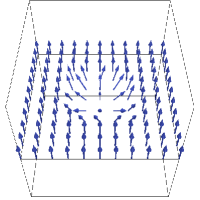
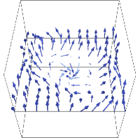
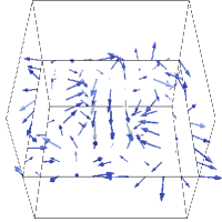
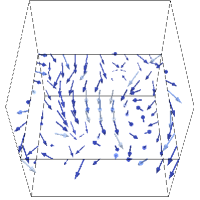
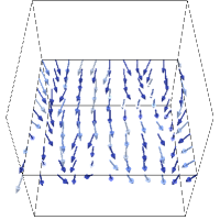
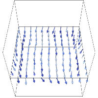
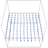
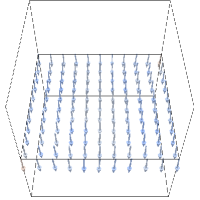
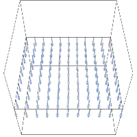
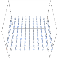
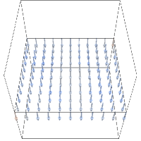
Figure 2. Slice of the magnetization $\boldsymbol{m}_{hk}(t_{i})$ at $[0,1]^{2}\times\{1/2\}$ for $i=0,\ldots,10$ with $t_{i}=0.2i$. The color of the vectors represents the magnitude $|\boldsymbol{m}_{hk}|$. We observe that the magnetization aligns itself with the initial magnetic field $\boldsymbol{H}^{0}$ by performing a damped precession.

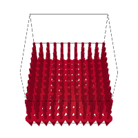
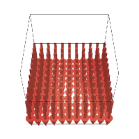
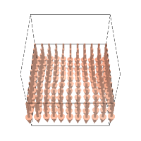
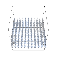
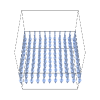
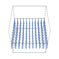
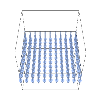
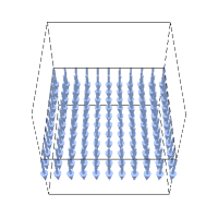
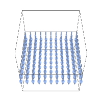
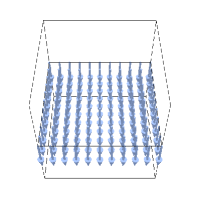
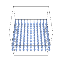
Figure 3. Slice of the magnetic field $\boldsymbol{H}_{hk}(t_{i})$ at $[0,1]^{2}\times\{1/2\}$ for $i=0,\ldots,10$ with $t_{i}=0.2i$. The color of the vectors represents the magnitude $|\boldsymbol{H}_{hk}|$. We observe only a slight movement in the middle of the cube combined with an overall reduction of field strength.

References

- [1] C. Abert, G. Hrkac, M. Page, D. Praetorius, M. Ruggeri, and D. Süss. Spin-polarized transport in ferromagnetic multilayers: An unconditionally convergent FEM integrator. Comput. Math. Appl., 68 (2014), 639–654.
- [2] R. A. Adams. Sobolev Spaces. Academic Press [A subsidiary of Harcourt Brace Jovanovich, Publishers], New York-London, 1975. Pure and Applied Mathematics, Vol. 65.
- [3] F. Alouges. A new finite element scheme for Landau-Lifchitz equations. Discrete Contin. Dyn. Syst. Ser. S, 1 (2008), 187–196.
- [4] F. Alouges, E. Kritsikis, J. Steiner, and J.-C. Toussaint. A convergent and precise finite element scheme for Landau-Lifschitz-Gilbert equation. Numer. Math., 128 (2014), 407–430.
- [5] F. Alouges and A. Soyeur. On global weak solutions for Landau-Lifshitz equations: existence and nonuniqueness. Nonlinear Anal., 18 (1992), 1071–1084.
- [6] M. Aurada, M. Feischl, and D. Praetorius. Convergence of some adaptive FEM-BEM coupling for elliptic but possibly nonlinear interface problems. ESAIM Math. Model. Numer. Anal., 46 (2012), 1147–1173.
- [7] L. Baňas, S. Bartels, and A. Prohl. A convergent implicit finite element discretization of the Maxwell–Landau–Lifshitz–Gilbert equation. SIAM J. Numer. Anal., 46 (2008), 1399–1422.
- [8] L. Baňas, M. Page, and D. Praetorius. A convergent linear finite element scheme for the Maxwell-Landau-Lifshitz-Gilbert equations. Electron. Trans. Numer. Anal., 44 (2015), 250–270.
- [9] S. Bartels. Projection-free approximation of geometrically constrained partial differential equations. Math. Comp., (2015).
- [10] S. Bartels, J. Ko, and A. Prohl. Numerical analysis of an explicit approximation scheme for the Landau-Lifshitz-Gilbert equation. Math. Comp., 77 (2008), 773–788.
- [11] S. Bartels and A. Prohl. Convergence of an implicit finite element method for the Landau-Lifshitz-Gilbert equation. SIAM J. Numer. Anal., 44 (2006), 1405–1419 (electronic).
- [12] J. Bergh and J. Löfström. Interpolation spaces. An introduction. Springer-Verlag, Berlin-New York, 1976. Grundlehren der Mathematischen Wissenschaften, No. 223.
- [13] A. Bossavit. Two dual formulations of the -D eddy-currents problem. COMPEL, 4 (1985), 103–116.
- [14] A. Buffa and P. Ciarlet, Jr. On traces for functional spaces related to Maxwell’s equations. I. An integration by parts formula in Lipschitz polyhedra. Math. Methods Appl. Sci., 24 (2001), 9–30.
- [15] A. Buffa and P. Ciarlet, Jr. On traces for functional spaces related to Maxwell’s equations. II. Hodge decompositions on the boundary of Lipschitz polyhedra and applications. Math. Methods Appl. Sci., 24 (2001), 31–48.
- [16] G. Carbou and P. Fabrie. Time average in micromagnetism. J. Differential Equations, 147 (1998), 383–409.
- [17] I. Cimrák. Existence, regularity and local uniqueness of the solutions to the Maxwell–Landau–Lifshitz system in three dimensions. J. Math. Anal. Appl., 329 (2007), 1080–1093.
- [18] I. Cimrák. A survey on the numerics and computations for the Landau-Lifshitz equation of micromagnetism. Arch. Comput. Methods Eng., 15 (2008), 277–309.
- [19] CTCMS. Mmmg: Micromagnetic Modeling Activity Group. http://www.ctcms.nist.gov/ rdm/mumag.org.html, .
- [20] M. Feischl and T. Tran. The eddy current–LLG equations – Part II: A priori error estimates. Research Report, UNSW, The University of New South Wales, 2016.
- [21] T. Gilbert. A Lagrangian formulation of the gyromagnetic equation of the magnetic field. Phys Rev, 100 (1955), 1243–1255.
- [22] M. Kružík and A. Prohl. Recent developments in the modeling, analysis, and numerics of ferromagnetism. SIAM Rev., 48 (2006), 439–483.
- [23] L. Landau and E. Lifschitz. On the theory of the dispersion of magnetic permeability in ferromagnetic bodies. Phys Z Sowjetunion, 8 (1935), 153–168.
- [24] K.-N. Le, M. Page, D. Praetorius, and T. Tran. On a decoupled linear FEM integrator for eddy-current-LLG. Appl. Anal., 94 (2015), 1051–1067.
- [25] K.-N. Le and T. Tran. A convergent finite element approximation for the quasi-static Maxwell-Landau-Lifshitz-Gilbert equations. Comput. Math. Appl., 66 (2013), 1389–1402.
- [26] J. L. Lions. Quelques Méthodes de Résolution des Problèmes aux Limites Non Linéaires. Dunod Gauthier-Villars, Paris, 1969.
- [27] A. Logg, K.-A. Mardal, and G. N. Wells, editors. Automated solution of differential equations by the finite element method, volume 84 of Lecture Notes in Computational Science and Engineering. Springer, Heidelberg, 2012. The FEniCS book.
- [28] P. Monk. Finite Element Methods for Maxwell’s equations. Numerical Mathematics and Scientific Computation. Oxford University Press, New York, 2003.
- [29] A. Prohl. Computational Micromagnetism. Advances in Numerical Mathematics. B. G. Teubner, Stuttgart, 2001.
- [30] W. Śmigaj, T. Betcke, S. Arridge, J. Phillips, and M. Schweiger. Solving boundary integral problems with BEM++. ACM Trans. Math. Software, 41 (2015), Art. 6, 40.
- [31] A. Visintin. On Landau-Lifshitz’ equations for ferromagnetism. Japan J. Appl. Math., 2 (1985), 69–84.