The Eddy Current–LLG Equations: FEM-BEM Coupling and A Priori Error Estimates

Abstract

We analyze a numerical method for the coupled system of the eddy current equations in ${\mathbb{R}}^{3}$ with the Landau-Lifshitz-Gilbert equation in a bounded domain. The unbounded domain is discretized by means of finite-element/boundary-element coupling. Even though the considered problem is strongly nonlinear, the numerical approach is constructed such that only two linear systems per time step have to be solved. We prove unconditional weak convergence (of a subsequence) of the finite-element solutions towards a weak solution. We establish a priori error estimates if a sufficiently smooth strong solution exists. Numerical experiments underlining the theoretical results are presented.

Primary 35Q40, 35K55, 35R60, 60H15, 65L60, 65L20, 65C30; Secondary 82D45

1 Introduction

This paper deals with the coupling of finite element and boundary element methods to solve the system of the eddy current equations in the whole 3D spatial space and the Landau-Lifshitz-Gilbert equation (LLG), the so-called ELLG system or equations. The system is also called the quasi-static Maxwell-LLG (MLLG) system.

The LLG is widely considered as a valid model of micromagnetic phenomena occurring in, e.g., magnetic sensors, recording heads, and magneto-resistive storage device [21, 24, 31]. Classical results concerning existence and non-uniqueness of solutions can be found in [5, 33]. In a ferro-magnetic material, magnetization is created or affected by external electro-magnetic fields. It is therefore necessary to augment the Maxwell system with the LLG, which describes the influence of a ferromagnet; see e.g. [19, 23, 33]. Existence, regularity and local uniqueness for the MLLG equations are studied in [18].

Throughout the literature, there are various works on numerical approximation methods for the LLG, ELLG, and MLLG equations [3, 4, 10, 11, 19, 25, 26] (the list is not exhausted), and even with the full Maxwell system on bounded domains [7, 8], and in the whole ${\mathbb{R}}^{3}$ [17]. Originating from the seminal work [3], the recent works [25, 26] consider a similar numeric integrator for a bounded domain. While the numerical integrator of [26] treated LLG and eddy current simultaneously per time step, [25] adapted an idea of [8] and decoupled the time-steps for LLG and the eddy current equation. Our approach follows [25].

This work studies the ELLG equations where we consider the electromagnetic field on the whole ${\mathbb{R}}^{3}$ and do not need to introduce artificial boundaries. Differently from [17] where the Faedo-Galerkin method is used to prove existence of weak solutions, we extend the analysis for the integrator used in [3, 25, 26] to a finite-element/boundary-element (FEM/BEM) discretization of the eddy current part on ${\mathbb{R}}^{3}$. This is inspired by the FEM/BEM coupling approach designed for the pure eddy current problem in [13], which allows us to treat unbounded domains without introducing artificial boundaries. Two approaches are proposed in [13]: the so-called “magnetic (or $\boldsymbol{H}$-based) approach” which eliminates the electric field, retaining only the magnetic field as the unknown in the eddy-current system, and the “electric (or $\boldsymbol{E}$-based) approach” which considers a primitive of the electric field as the only unknown. The coupling of the eddy-current system with the LLG dictates that the first approach is more appropriate, because this coupling involves the magnetic field in the LLG equation rather than the electric field; see Eq. 1.

The main results of this work are weak convergence of the discrete approximation towards a weak solution without any condition on the space and time discretization as well as a priori error estimates under the condition that the exact (strong) solution is sufficiently smooth. In particular, the first result implies the existence of weak solutions, whereas the latter shows that the smooth strong solution is unique. To the best of our knowledge, no such results for the tangent plane scheme have been proved for the LLG equation. Therefore, we present the proof for this equation in a separate section, before proving the result for the ELLG system.

As in [1], the proof is facilitated by use of an idea of [9] for the harmonic map heat (analyzed for LLG in [1]), which avoids the normalization of the solution in each time-step, and therefore allows us to use a linear update formula. This also enables us to consider general quasi-uniform triangulations for discretization and removes the requirement for very shape-regular elements (all dihedral angles smaller than $\pi/2$) present in previous works on this topic.

The remainder of this work is organized as follows. Section 2 introduces the coupled problem and the notation, presents the numerical algorithm, and states the main results of this paper. Section 3 is devoted to the proofs of these main results. Numerical results are presented in Section 4. The final section, the Appendix, contains the proofs of some rather elementary or well-known results.

2 Model Problem & Main Results

2.1 The problem

Consider a bounded Lipschitz domain $D\subset{\mathbb{R}}^{3}$ with connected boundary $\Gamma$ having the outward normal vector $\boldsymbol{n}$. We define $D^{\ast}:={\mathbb{R}}^{3}\setminus\overline{D}$, $D_{T}:=(0,T)\times D$, $\Gamma_{T}:=(0,T)\times\Gamma$, $D_{T}^{\ast}:=(0,T)\times D^{\ast}$, and ${\mathbb{R}}^{3}_{T}:=(0,T)\times{\mathbb{R}}^{3}$ for $T>0$. For simplicity, we assume that $D^{\ast}$ is simply connected. We start with the quasi-static approximation of the full Maxwell-LLG system from [33] which reads as

(1a) $$\boldsymbol{m}_{t}-\alpha\boldsymbol{m}\times\boldsymbol{m}_{t} =-\boldsymbol{m}\times\boldsymbol{H}_{\rm eff} \quad\text{in }D_{T},$$

(1b) $$\sigma\boldsymbol{E}-\nabla\times\boldsymbol{H} =0 \quad\text{in }{\mathbb{R}}^{3}_{T},$$

(1c) $$\mu_{0}\boldsymbol{H}_{t}+\nabla\times\boldsymbol{E} =-\mu_{0}\widetilde{\boldsymbol{m}}_{t} \quad\text{in }{\mathbb{R}}^{3}_{T},$$

(1d) $${\rm div}(\boldsymbol{H}+\widetilde{\boldsymbol{m}}) =0 \quad\text{in }{\mathbb{R}}^{3}_{T},$$

(1e) $${\rm div}(\boldsymbol{E}) =0 \quad\text{in }D^{\ast}_{T},$$

where $\widetilde{\boldsymbol{m}}$ is the zero extension of $\boldsymbol{m}$ to ${\mathbb{R}}^{3}$ and $\boldsymbol{H}_{\rm eff}$ is the effective field defined by $\boldsymbol{H}_{\rm eff}=C_{e}\Delta\boldsymbol{m}+\boldsymbol{H}$ for some constant $C_{e}>0$. Here the parameter $\alpha>0$ and permeability $\mu_{0}\geq 0$ are constants, whereas the conductivity $\sigma$ takes a constant positive value in $D$ and the zero value in $D^{\ast}$. Equation 1d is understood in the distributional sense because there is a jump of $\widetilde{\boldsymbol{m}}$ across $\Gamma$. Note that $\boldsymbol{H}_{\rm eff}$ contains only the high order term for simplicity. A refined analysis might also allow us to include lower order terms (anisotropy, exterior applied field) as done in [14].

It follows from Eq. 1a that $|\boldsymbol{m}|$ is constant. We follow the usual practice to normalize $|\boldsymbol{m}|$ (and thus the same condition is required for $|\boldsymbol{m}^{0}|$). The following conditions are imposed on the solutions of Eq. 1:

(2a) $$\partial_{n}\boldsymbol{m} =0 \quad\text{on }\Gamma_{T},$$

(2b) $$|\boldsymbol{m}| =1 \quad\text{in }D_{T},$$

(2c) $$\boldsymbol{m}(0,\cdot) =\boldsymbol{m}^{0} \quad\text{in }D,$$

(2d) $$\boldsymbol{H}(0,\cdot) =\boldsymbol{H}^{0} \quad\text{in }{\mathbb{R}}^{3},$$

(2e) $$|\boldsymbol{H}(t,x)| =\mathcal{O}(|x|^{-1}) \quad\text{as }|x|\to\infty,$$

where $\partial_{n}$ denotes the normal derivative. The initial data $\boldsymbol{m}^{0}$ and $\boldsymbol{H}^{0}$ satisfy $|\boldsymbol{m}^{0}|=1$ in $D$ and

(3) $$\begin{split}{\rm div}(\boldsymbol{H}^{0}+\widetilde{\boldsymbol{m}}^{0})&=0\quad\text{in }{\mathbb{R}}^{3}.\end{split}$$

The condition Eq. 2b together with basic properties of the cross product leads to the following equivalent formulation of Eq. 1a:

(4) $$\alpha\boldsymbol{m}_{t}+\boldsymbol{m}\times\boldsymbol{m}_{t}=\boldsymbol{H}_{\rm eff}-(\boldsymbol{m}\cdot\boldsymbol{H}_{\rm eff})\boldsymbol{m}\quad\text{in }D_{T}.$$

Below, we focus on an $\boldsymbol{H}$-based formulation of the problem. It is possible to recover $\boldsymbol{E}$ once $\boldsymbol{H}$ and $\boldsymbol{m}$ are known; see Eq. 12

2.2 Function spaces and notations

Before introducing the concept of weak solutions to problem Eq. 1–Eq. 2 we need the following definitions of function spaces. Let ${\mathbb{L}}^{2}{(D}):=L^{2}(D;{\mathbb{R}}^{3})$ and ${\mathbb{H}}({\rm curl},D):=\big{\{}\boldsymbol{w}\in{\mathbb{L}}^{2}{(D})\,:\,\nabla\times\boldsymbol{w}\in{\mathbb{L}}^{2}{(D})\big{\}}$. We define $H^{1/2}(\Gamma)$ as the usual trace space of $H^{1}(D)$ and define its dual space $H^{-1/2}(\Gamma)$ by extending the $L^{2}$-inner product on $\Gamma$. For convenience we denote

$${\mathcal{X}}:=\big{\{}(\boldsymbol{\xi},\zeta)\in{\mathbb{H}}({\rm curl},D)\times H^{1/2}(\Gamma)\,:\,\boldsymbol{n}\times\boldsymbol{\xi}|_{\Gamma}=\boldsymbol{n}\times\nabla_{\Gamma}\zeta\text{ in the sense of traces}\big{\}}.$$

Recall that $\boldsymbol{n}\times\boldsymbol{\xi}|_{\Gamma}$ is the tangential trace (or twisted tangential trace) of $\boldsymbol{\xi}$, and $\nabla_{\Gamma}\zeta$ is the surface gradient of $\zeta$. Their definitions and properties can be found in [15, 16].

Finally, if $X$ is a normed vector space then, for $m\geq 0$ and $p\in{\mathbb{N}}\cup\{\infty\}$, $L^{2}(0,T;X)$, $H^{m}(0,T;X)$, and $W^{m,p}(0,T;X)$ denote the usual Lebesgue and Sobolev spaces of functions defined on $(0,T)$ and taking values in $X$.

We finish this subsection with the clarification of the meaning of the cross product between different mathematical objects. For any vector functions $\boldsymbol{u},\boldsymbol{v},\boldsymbol{w}$ we denote

$$\boldsymbol{u}\times\nabla\boldsymbol{v}:=\left(\boldsymbol{u}\times\frac{\partial\boldsymbol{v}}{\partial x_{1}},\boldsymbol{u}\times\frac{\partial\boldsymbol{v}}{\partial x_{2}},\boldsymbol{u}\times\frac{\partial\boldsymbol{v}}{\partial x_{3}}\right),\quad\nabla\boldsymbol{u}\times\nabla\boldsymbol{v}:=\sum_{i=1}^{3}\frac{\partial\boldsymbol{u}}{\partial x_{i}}\times\frac{\partial\boldsymbol{v}}{\partial x_{i}}$$

and

$$(\boldsymbol{u}\times\nabla\boldsymbol{v})\cdot\nabla\boldsymbol{w}:=\sum_{i=1}^{3}\left(\boldsymbol{u}\times\frac{\partial\boldsymbol{v}}{\partial x_{i}}\right)\cdot\frac{\partial\boldsymbol{w}}{\partial x_{i}}.$$

2.3 Weak solutions

A weak formulation for Eq. 1a is well-known, see e.g. [3, 26]. Indeed, by multiplying Eq. 4 by $\boldsymbol{\phi}\in C^{\infty}(D_{T};{\mathbb{R}}^{3})$, using integration by parts, we deduce

$$\alpha\langle\boldsymbol{m}_{t}\,,\,\boldsymbol{m}\times\boldsymbol{\phi}\rangle_{D_{T}}+\langle\boldsymbol{m}\times\boldsymbol{m}_{t}\,,\,\boldsymbol{m}\times\boldsymbol{\phi}\rangle_{D_{T}}+C_{e}\langle\nabla\boldsymbol{m}\,,\,\nabla(\boldsymbol{m}\times\boldsymbol{\phi})\rangle_{D_{T}}=\langle\boldsymbol{H}\,,\,\boldsymbol{m}\times\boldsymbol{\phi}\rangle_{D_{T}}.$$

To tackle the eddy current equations on ${\mathbb{R}}^{3}$, we aim to employ FE/BE coupling methods. To that end, we employ the magnetic approach from [13], which eventually results in a variant of the Trifou-discretization of the eddy-current Maxwell equations.

Multiplying Eq. 1c by $\boldsymbol{\xi}\in C^{\infty}(D,{\mathbb{R}}^{3})$ satisfying $\nabla\times\boldsymbol{\xi}=0$ in $D^{\ast}$, integrating over ${\mathbb{R}}^{3}$, and using integration by parts, we obtain for almost all $t\in[0,T]$

$$\mu_{0}\langle\boldsymbol{H}_{t}(t)\,,\,\boldsymbol{\xi}\rangle_{{\mathbb{R}}^{3}}+\langle\boldsymbol{E}(t)\,,\,\nabla\times\boldsymbol{\xi}\rangle_{{\mathbb{R}}^{3}}=-\mu_{0}\langle\boldsymbol{m}_{t}(t)\,,\,\boldsymbol{\xi}\rangle_{D}.$$

Using $\nabla\times\boldsymbol{\xi}=0$ in $D^{\ast}$ and Eq. 1b we deduce

$$\mu_{0}\langle\boldsymbol{H}_{t}(t)\,,\,\boldsymbol{\xi}\rangle_{{\mathbb{R}}^{3}}+\sigma^{-1}\langle\nabla\times\boldsymbol{H}(t)\,,\,\nabla\times\boldsymbol{\xi}\rangle_{D}=-\mu_{0}\langle\boldsymbol{m}_{t}(t)\,,\,\boldsymbol{\xi}\rangle_{D}.$$

Since $\nabla\times\boldsymbol{H}=\nabla\times\boldsymbol{\xi}=0$ in $D^{\ast}$ and $D^{\ast}$ is simply connected by definition (a workaround for non-simply connected $D^{\ast}$ is presented in [22]), there exists $\varphi$ and $\zeta$ such that $\boldsymbol{H}=\nabla\varphi$ and $\boldsymbol{\xi}=\nabla\zeta$ in $D^{\ast}$. Therefore, the above equation can be rewritten as

$$\mu_{0}\langle\boldsymbol{H}_{t}(t)\,,\,\boldsymbol{\xi}\rangle_{D}+\mu_{0}\langle\nabla\varphi_{t}(t)\,,\,\nabla\zeta\rangle_{D^{\ast}}+\sigma^{-1}\langle\nabla\times\boldsymbol{H}(t)\,,\,\nabla\times\boldsymbol{\xi}\rangle_{D}=-\mu_{0}\langle\boldsymbol{m}_{t}(t)\,,\,\boldsymbol{\xi}\rangle_{D}.$$

Since Eq. 1d implies ${\rm div}(\boldsymbol{H})=0$ in $D^{\ast}$, we have $\Delta\varphi=0$ in $D^{\ast}$, so that (formally) $\Delta\varphi_{t}=0$ in $D^{\ast}$. Hence integration by parts yields

(5) $$\mu_{0}\langle\boldsymbol{H}_{t}(t)\,,\,\boldsymbol{\xi}\rangle_{D}-\mu_{0}\langle\partial_{n}^{+}\varphi_{t}(t)\,,\,\zeta\rangle_{\Gamma}+\sigma^{-1}\langle\nabla\times\boldsymbol{H}(t)\,,\,\nabla\times\boldsymbol{\xi}\rangle_{D}=-\mu_{0}\langle\boldsymbol{m}_{t}(t)\,,\,\boldsymbol{\xi}\rangle_{D},$$

where $\partial_{n}^{+}$ is the exterior Neumann trace operator with the limit taken from $D^{\ast}$. The advantage of the above formulation is that no integration over the unbounded domain $D^{\ast}$ is required. The exterior Neumann trace $\partial_{n}^{+}\varphi_{t}$ can be computed from the exterior Dirichlet trace $\lambda$ of $\varphi$ by using the Dirichlet-to-Neumann operator $\mathfrak{S}$, which is defined as follows.

Let $\gamma^{-}$ be the interior Dirichlet trace operator and $\partial_{n}^{-}$ be the interior normal derivative or Neumann trace operator. (The $-$ sign indicates that the trace is taken from $D$.) Recalling the fundamental solution of the Laplacian $G(x,y):=1/(4\pi|x-y|)$, we introduce the following integral operators defined formally on $\Gamma$ as

$$\mathfrak{V}(\lambda):=\gamma^{-}\overline{\mathfrak{V}}(\lambda),\quad\mathfrak{K}(\lambda):=\gamma^{-}\overline{\mathfrak{K}}(\lambda)+\mbox{$\frac{1}{2}$},\quad\text{and}\quad\mathfrak{W}(\lambda):=-\partial_{n}^{-}\overline{\mathfrak{K}}(\lambda),$$

where, for $x\notin\Gamma$,

$$\overline{\mathfrak{V}}(\lambda)(x):=\int_{\Gamma}G(x,y)\lambda(y)\,ds_{y}\quad\text{and}\quad\overline{\mathfrak{K}}(\lambda)(x):=\int_{\Gamma}\partial_{n(y)}G(x,y)\lambda(y)\,ds_{y},$$

see, e.g., [29] for further details. Moreover, let $\mathfrak{K}^{\prime}$ denote the adjoint operator of $\mathfrak{K}$ with respect to the extended $L^{2}$-inner product. Then the exterior Dirichlet-to-Neumann map $\mathfrak{S}\colon H^{1/2}(\Gamma)\to H^{-1/2}(\Gamma)$ can be represented as

(6) $$\mathfrak{S}=-\mathfrak{V}^{-1}(1/2-\mathfrak{K}).$$

Another representation is

(7) $$\mathfrak{S}=-(1/2-\mathfrak{K}^{\prime})\mathfrak{V}^{-1}(1/2-\mathfrak{K})-\mathfrak{W}.$$

Recall that $\varphi$ satisfies $\boldsymbol{H}=\nabla\varphi$ in $D^{\ast}$. We can choose $\varphi$ satisfying $\varphi(x)=O(|x|^{-1})$ as $|x|\to\infty$. Now if $\lambda=\gamma^{+}\varphi$ then $\lambda_{t}=\gamma^{+}\varphi_{t}$. Since $\Delta\varphi=\Delta\varphi_{t}=0$ in $D^{\ast}$, and since the exterior Laplace problem has a unique solution we have $\mathfrak{S}\lambda=\partial_{n}^{+}\varphi$ and $\mathfrak{S}\lambda_{t}=\partial_{n}^{+}\varphi_{t}$. Hence Eq. 5 can be rewritten as

(8) $$\langle\boldsymbol{H}_{t}(t)\,,\,\boldsymbol{\xi}\rangle_{D}-\langle\mathfrak{S}\lambda_{t}(t)\,,\,\zeta\rangle_{\Gamma}+\mu_{0}^{-1}\sigma^{-1}\langle\nabla\times\boldsymbol{H}(t)\,,\,\nabla\times\boldsymbol{\xi}\rangle_{D}=-\langle\boldsymbol{m}_{t}(t)\,,\,\boldsymbol{\xi}\rangle_{D}.$$

We remark that if $\nabla_{\Gamma}$ denotes the surface gradient operator on $\Gamma$ then it is well-known that $\nabla_{\Gamma}\lambda=(\nabla\varphi)|_{\Gamma}-(\partial_{n}^{+}\varphi)\boldsymbol{n}=\boldsymbol{H}|_{\Gamma}-(\partial_{n}^{+}\varphi)\boldsymbol{n};$ see e.g. [30, Section 3.4]. Hence $\boldsymbol{n}\times\nabla_{\Gamma}\lambda=\boldsymbol{n}\times\boldsymbol{H}|_{\Gamma}$.

The above analysis prompts us to define the following weak formulation.

Definition 2.1.

A triple $(\boldsymbol{m},\boldsymbol{H},\lambda)$ satisfying

$$\boldsymbol{m} \in{\mathbb{H}}^{1}{(D_{T}})\quad\text{and}\quad\boldsymbol{m}_{t}|_{\Gamma_{T}}\in L^{2}(0,T;H^{-1/2}(\Gamma)),$$

$$\boldsymbol{H} \in L^{2}(0,T;{\mathbb{H}}({\rm curl},D))\cap H^{1}(0,T;{\mathbb{L}}^{2}{(D})),$$

$$\lambda \in H^{1}(0,T;H^{1/2}(\Gamma))$$

is called a weak solution to Eq. 1–Eq. 2 if the following statements hold

1. $|\boldsymbol{m}|=1$ almost everywhere in $D_{T}$;

2. $\boldsymbol{m}(0,\cdot)=\boldsymbol{m}^{0}$, $\boldsymbol{H}(0,\cdot)=\boldsymbol{H}^{0}$, and $\lambda(0,\cdot)=\gamma^{+}\varphi^{0}$ where $\varphi^{0}$ is a scalar function satisfies $\boldsymbol{H}^{0}=\nabla\varphi^{0}$ in $D^{\ast}$ (the assumption Eq. 3 ensures the existence of $\varphi^{0}$);

3. For all $\boldsymbol{\phi}\in C^{\infty}(D_{T};{\mathbb{R}}^{3})$

   $$\alpha\langle\boldsymbol{m}_{t}\,,\,\boldsymbol{m}\times\boldsymbol{\phi}\rangle_{D_{T}} +\langle\boldsymbol{m}\times\boldsymbol{m}_{t}\,,\,\boldsymbol{m}\times\boldsymbol{\phi}\rangle_{D_{T}}+C_{e}\langle\nabla\boldsymbol{m}\,,\,\nabla(\boldsymbol{m}\times\boldsymbol{\phi})\rangle_{D_{T}}$$

   (9a) $$=\langle\boldsymbol{H}\,,\,\boldsymbol{m}\times\boldsymbol{\phi}\rangle_{D_{T}};$$

4. There holds $\boldsymbol{n}\times\nabla_{\Gamma}\lambda=\boldsymbol{n}\times\boldsymbol{H}|_{\Gamma}$ in the sense of traces;

5. For $\boldsymbol{\xi}\in C^{\infty}(D;{\mathbb{R}}^{3})$ and $\zeta\in C^{\infty}(\Gamma)$ satisfying $\boldsymbol{n}\times\boldsymbol{\xi}|_{\Gamma}=\boldsymbol{n}\times\nabla_{\Gamma}\zeta$ in the sense of traces

   (9b) $$\langle\boldsymbol{H}_{t}\,,\,\boldsymbol{\xi}\rangle_{D_{T}}-\langle\mathfrak{S}\lambda_{t}\,,\,\zeta\rangle_{\Gamma_{T}}+\sigma^{-1}\mu_{0}^{-1}\langle\nabla\times\boldsymbol{H}\,,\,\nabla\times\boldsymbol{\xi}\rangle_{D_{T}} =-\langle\boldsymbol{m}_{t}\,,\,\boldsymbol{\xi}\rangle_{D_{T}};$$

6. For almost all $t\in[0,T]$

   $$\|\nabla\boldsymbol{m}(t)\|_{{\mathbb{L}}^{2}{(D})}^{2}+\|\boldsymbol{H}(t)\|_{{\mathbb{H}}({\rm curl},D)}^{2}+\|\lambda(t)\|_{H^{1/2}(\Gamma)}^{2}$$

   (10) $$+\|\boldsymbol{m}_{t}\|_{{\mathbb{L}}^{2}{(D_{t}})}^{2}+\|\boldsymbol{H}_{t}\|_{{\mathbb{L}}^{2}{(D_{t}})}^{2}+\|\lambda_{t}\|_{H^{1/2}(\Gamma_{t})}^{2}\leq C,$$

   where the constant $C>0$ is independent of $t$.

A triple $(\boldsymbol{m},\boldsymbol{H},\lambda)$ is called a strong solution of the ELLG system Eq. 1–Eq. 2 if it is a weak solution and additionally it is sufficiently smooth such that Eq. 4 is satisfied in the strong sense.

Remark 2.2.

A refinement of the arguments in Theorem 2.6 would allow us to prove that the weak solutions which appear as limits of the approximations from Algorithm 2.5, are energy dissipative, i.e.,

$$\frac{C_{e}}{2}\|\nabla\boldsymbol{m}(t)\|_{{\mathbb{L}}^{2}{(D})}^{2} +\|\boldsymbol{H}(t)\|_{{\mathbb{L}}^{2}{(D})}^{2}-\langle\mathfrak{S}\lambda(t)\,,\,\lambda(t)\rangle_{\Gamma}$$

$$\leq\frac{C_{e}}{2}\|\nabla\boldsymbol{m}^{0}\|_{{\mathbb{L}}^{2}{(D})}^{2}+\|\boldsymbol{H}^{0}\|_{{\mathbb{L}}^{2}{(D})}^{2}-\langle\mathfrak{S}\lambda(0)\,,\,\lambda(0)\rangle_{\Gamma}$$

for all $t\in[0,T]$. The proof works along the lines of [1, Theorem 24] or [14, Appendix A] and is therefore omitted.

The reason we integrate over $[0,T]$ in Eq. 8 to have Eq. 9b is to facilitate the passing to the limit in the proof of the main theorem. The following lemma justifies the above definition.

Lemma 2.3.

Let $(\boldsymbol{m},\boldsymbol{H},\boldsymbol{E})$ be a strong solution of Eq. 1–Eq. 2. If $\varphi\in H(0,T;H^{1}(D^{\ast}))$ satisfies $\nabla\varphi=\boldsymbol{H}|_{D^{\ast}_{T}}$, and if $\lambda:=\gamma^{+}\varphi$, then the triple $(\boldsymbol{m},\boldsymbol{H}|_{D_{T}},\lambda)$ is a weak solution in the sense of Definition 2.1. Conversely, given a weak solution $(\boldsymbol{m},\boldsymbol{H}|_{D_{T}},\lambda)$ in the sense of Definition 2.1, let $\varphi$ be the solution of

(11) $$\Delta\varphi=0\text{ in }D^{\ast},\quad\varphi=\lambda\text{ on }\Gamma,\quad\varphi(x)=O(|x|^{-1})\text{ as }|x|\to\infty$$

and define $\boldsymbol{H}|_{D_{T}^{\star}}:=\nabla\phi$ as well as $\boldsymbol{E}$ via $\boldsymbol{E}=\sigma^{-1}(\nabla\times\boldsymbol{H}|_{D_{T}})$ in $D_{T}$ and outside of $D_{T}$ as the solution of

(12a) $$\nabla\times\boldsymbol{E} =-\mu_{0}\boldsymbol{H}_{t} \quad\text{in }D_{T}^{\ast},$$

(12b) $${\rm div}(\boldsymbol{E}) =0 \quad\text{in }D_{T}^{\ast},$$

(12c) $$\boldsymbol{n}\times\boldsymbol{E}|_{D_{T}^{\ast}} =\boldsymbol{n}\times\boldsymbol{E}|_{D_{T}} \quad\text{on }\Gamma_{T}.$$

If $\boldsymbol{m}$, $\boldsymbol{H}$, and $\boldsymbol{E}$ are sufficiently smooth, $(\boldsymbol{m},\boldsymbol{H},\boldsymbol{E})$ is a strong solution of Eq. 1–Eq. 2.

Proof 2.4.

We follow [13]. Assume that $(\boldsymbol{m},\boldsymbol{H},\boldsymbol{E})$ satisfies Eq. 1–Eq. 2. Then, Item 1, Item 2 and Item 6 in Definition 2.1 hold, noting Eq. 3. Item 3, Item 4 and Item 5 also hold due to the analysis above Definition 2.1. The converse is also true due to the well-posedness of Eq. 12 as stated in [13, Equation (15)].

Remark 2.5.

The solution $\varphi$ to Eq. 11 can be represented as $\varphi=(1/2+\mathfrak{K})\lambda-\mathfrak{V}\mathfrak{S}\lambda.$

The next subsection defines the spaces and functions to be used in the approximation of the weak solution the sense of Definition 2.1.

2.4 Discrete spaces and functions

For time discretization, we use a uniform partition $0\leq t_{i}\leq T$, $i=0,\ldots,N$ with $t_{i}:=ik$ and $k:=T/N$. The spatial discretization is determined by a (shape) regular triangulation ${\mathcal{T}}_{h}$ of $D$ into compact tetrahedra $\tau\in{\mathcal{T}}_{h}$ with diameter $h_{\tau}/C\leq h\leq C|\tau|^{1/3}$ for some uniform constant $C>0$. Denoting by ${\mathcal{N}}_{h}$ the set of nodes of ${\mathcal{T}}_{h}$, we define the following spaces

$$\SS^{1}({\mathcal{T}}_{h}) :=\big{\{}\phi_{h}\in C(D)\,:\,\phi_{h}|\tau\in{\mathcal{P}}^{1}(\tau)\text{ for all }\tau\in{\mathcal{T}}_{h}\big{\}},$$

$${\mathcal{K}}_{\boldsymbol{\phi}_{h}} :=\big{\{}\boldsymbol{\psi}_{h}\in\SS^{1}({\mathcal{T}}_{h})^{3}\,:\,\boldsymbol{\psi}_{h}(z)\cdot\boldsymbol{\phi}_{h}(z)=0\text{ for all }z\in{\mathcal{N}}_{h}\big{\}},\quad\boldsymbol{\phi}_{h}\in\SS^{1}({\mathcal{T}}_{h})^{3},$$

where ${\mathcal{P}}^{1}(\tau)$ is the space of polynomials of degree at most 1 on $\tau$.

For the discretization of Eq. 9b, we employ the space ${\mathcal{N}}{\mathcal{D}}^{1}({\mathcal{T}}_{h})$ of first order Nédélec (edge) elements for $\boldsymbol{H}$ and and the space $\SS^{1}({\mathcal{T}}_{h}|_{\Gamma})$ for $\lambda$. Here ${\mathcal{T}}_{h}|_{\Gamma}$ denotes the restriction of the triangulation to the boundary $\Gamma$. It follows from Item 4 in Definition 2.1 that for each $t\in[0,T]$, the pair $(\boldsymbol{H}(t),\lambda(t))\in{\mathcal{X}}$. We approximate the space ${\mathcal{X}}$ by

$${\mathcal{X}}_{h}:=\big{\{}(\boldsymbol{\xi},\zeta)\in{\mathcal{N}}{\mathcal{D}}^{1}({\mathcal{T}}_{h})\times\SS^{1}({\mathcal{T}}_{h}|_{\Gamma})\,:\,\boldsymbol{n}\times\nabla_{\Gamma}\zeta=\boldsymbol{n}\times\boldsymbol{\xi}|_{\Gamma}\big{\}}.$$

To ensure the condition $\boldsymbol{n}\times\nabla_{\Gamma}\zeta=\boldsymbol{n}\times\boldsymbol{\xi}|_{\Gamma}$, we observe the following. For any $\zeta\in\SS^{1}({\mathcal{T}}_{h}|_{\Gamma})$, if $e$ denotes an edge of ${\mathcal{T}}_{h}$ on $\Gamma$, then $\int_{e}\boldsymbol{\xi}\cdot\boldsymbol{\tau}\,ds=\int_{e}\nabla\zeta\cdot\boldsymbol{\tau}\,ds=\zeta(z_{0})-\zeta(z_{1})$, where $\boldsymbol{\tau}$ is the unit direction vector on $e$, and $z_{0},z_{1}$ are the endpoints of $e$. Thus, taking as degrees of freedom all interior edges of ${\mathcal{T}}_{h}$ (i.e. $\int_{e_{i}}\boldsymbol{\xi}\cdot\boldsymbol{\tau}\,ds$) as well as all nodes of ${\mathcal{T}}_{h}|_{\Gamma}$ (i.e. $\zeta(z_{i})$), we fully determine a function pair $(\boldsymbol{\xi},\zeta)\in{\mathcal{X}}_{h}$. Due to the considerations above, it is clear that the above space can be implemented directly without use of Lagrange multipliers or other extra equations.

The density properties of the finite element spaces $\{{\mathcal{X}}_{h}\}_{h>0}$ are shown in Subsection 3.1; see Lemma 3.1.

Given functions $\boldsymbol{w}_{h}^{i}\colon D\to{\mathbb{R}}^{d}$, $d\in{\mathbb{N}}$, for all $i=0,\ldots,N$ we define for all $t\in[t_{i},t_{i+1}]$

$$\boldsymbol{w}_{hk}(t):=\frac{t_{i+1}-t}{k}\boldsymbol{w}_{h}^{i}+\frac{t-t_{i}}{k}\boldsymbol{w}_{h}^{i+1},\quad\boldsymbol{w}_{hk}^{-}(t):=\boldsymbol{w}_{h}^{i},\quad\boldsymbol{w}_{hk}^{+}(t):=\boldsymbol{w}_{h}^{i+1}.$$

Moreover, we define

(13) $$d_{t}\boldsymbol{w}_{h}^{i+1}:=\frac{\boldsymbol{w}_{h}^{i+1}-\boldsymbol{w}_{h}^{i}}{k}\quad\text{for all }i=0,\ldots,N-1.$$

Finally, we denote by $\Pi_{\SS}$ the usual interpolation operator on $\SS^{1}({\mathcal{T}}_{h})$.We are now ready to present the algorithm to compute approximate solutions to problem Eq. 1–Eq. 2.

2.5 Numerical algorithm

In the sequel, when there is no confusion we use the same notation $\boldsymbol{H}$ for the restriction of $\boldsymbol{H}\colon{\mathbb{R}}^{3}_{T}\to{\mathbb{R}}^{3}$ to the domain $D_{T}$.

Input: Initial data $\boldsymbol{m}^{0}_{h}\in\SS^{1}({\mathcal{T}}_{h})^{3}$, $(\boldsymbol{H}^{0}_{h},\lambda_{h}^{0})\in{\mathcal{X}}_{h}$, and parameter $\theta\in[0,1]$.

For $i=0,\ldots,N-1$ do:

1. Compute the unique function $\boldsymbol{v}^{i}_{h}\in{\mathcal{K}}_{\boldsymbol{m}_{h}^{i}}$ satisfying for all $\boldsymbol{\phi}_{h}\in{\mathcal{K}}_{\boldsymbol{m}_{h}^{i}}$

   (14) $$\begin{split}\alpha\langle\boldsymbol{v}_{h}^{i}\,,\,\boldsymbol{\phi}_{h}\rangle_{D}&+\langle\boldsymbol{m}_{h}^{i}\times\boldsymbol{v}_{h}^{i}\,,\,\boldsymbol{\phi}_{h}\rangle_{D}+C_{e}\theta k\langle\nabla\boldsymbol{v}_{h}^{i}\,,\,\nabla\boldsymbol{\phi}_{h}\rangle_{D}\\ &=-C_{e}\langle\nabla\boldsymbol{m}_{h}^{i}\,,\,\nabla\boldsymbol{\phi}_{h}\rangle_{D}+\langle\boldsymbol{H}_{h}^{i}\,,\,\boldsymbol{\phi}_{h}\rangle_{D}.\end{split}$$

2. Define $\boldsymbol{m}_{h}^{i+1}\in\SS^{1}({\mathcal{T}}_{h})^{3}$ nodewise by

   (15) $$\boldsymbol{m}_{h}^{i+1}(z)=\boldsymbol{m}_{h}^{i}(z)+k\boldsymbol{v}_{h}^{i}(z)\quad\text{for all }z\in{\mathcal{N}}_{h}.$$

3. Compute the unique functions $(\boldsymbol{H}_{h}^{i+1},\lambda_{h}^{i+1})\in{\mathcal{X}}_{h}$ satisfying for all $(\boldsymbol{\xi}_{h},\zeta_{h})\in{\mathcal{X}}_{h}$

   $$\langle d_{t}\boldsymbol{H}_{h}^{i+1}\,,\,\boldsymbol{\xi}_{h}\rangle_{D} -\langle d_{t}\mathfrak{S}_{h}\lambda_{h}^{i+1}\,,\,\zeta_{h}\rangle_{\Gamma}+\sigma^{-1}\mu_{0}^{-1}\langle\nabla\times\boldsymbol{H}_{h}^{i+1}\,,\,\nabla\times\boldsymbol{\xi}_{h}\rangle_{D}$$

   (16) $$=-\langle\boldsymbol{v}_{h}^{i}\,,\,\boldsymbol{\xi}_{h}\rangle_{D},$$

   where $\mathfrak{S}_{h}\colon H^{1/2}(\Gamma)\to\SS^{1}({\mathcal{T}}_{h}|_{\Gamma})$ is the discrete Dirichlet-to-Neumann operator to be defined later.

Output: Approximations $(\boldsymbol{m}_{h}^{i},\boldsymbol{H}_{h}^{i},\lambda_{h}^{i})$ for all $i=0,\ldots,N$.

The linear formula Eq. 15 was introduced in [9] for harmonic map heat flow and adapted for LLG in [1]. As already observed in [25, 8] (for bounded domains), we note that the linear systems (14) and (3) are decoupled and can be solved successively. Item 3 requires the computation of $\mathfrak{S}_{h}\lambda$ for any $\lambda\in H^{1/2}(\Gamma)$. This is done by use of the boundary element method. Let $\mu\in H^{-1/2}(\Gamma)$ and $\mu_{h}\in{\mathcal{P}}^{0}({\mathcal{T}}_{h}|_{\Gamma})$ be, respectively, the solution of

(17) $$\mathfrak{V}\mu=(\mathfrak{K}-1/2)\lambda\quad\text{and}\quad\langle\mathfrak{V}\mu_{h}\,,\,\nu_{h}\rangle_{\Gamma}=\langle(\mathfrak{K}-1/2)\lambda\,,\,\nu_{h}\rangle_{\Gamma}\quad\forall\nu_{h}\in{\mathcal{P}}^{0}({\mathcal{T}}_{h}|_{\Gamma}),$$

where ${\mathcal{P}}^{0}({\mathcal{T}}_{h}|_{\Gamma})$ is the space of piecewise-constant functions on ${\mathcal{T}}_{h}|_{\Gamma}$.

If the representation Eq. 6 of $\mathfrak{S}$ is used, then $\mathfrak{S}\lambda=\mu$, and we can uniquely define $\mathfrak{S}_{h}\lambda$ by solving

(18) $$\langle\mathfrak{S}_{h}\lambda\,,\,\zeta_{h}\rangle_{\Gamma}=\langle\mu_{h}\,,\,\zeta_{h}\rangle_{\Gamma}\quad\forall\zeta_{h}\in\SS^{1}({\mathcal{T}}_{h}|_{\Gamma}).$$

This is known as the Johnson-Nédélec coupling.

If we use the representation Eq. 7 for $\mathfrak{S}\lambda$ then $\mathfrak{S}\lambda=(1/2-\mathfrak{K}^{\prime})\mu-\mathfrak{W}\lambda$. In this case we can uniquely define $\mathfrak{S}_{h}\lambda$ by solving

(19) $$\langle\mathfrak{S}_{h}\lambda\,,\,\zeta_{h}\rangle_{\Gamma}=\langle(1/2-\mathfrak{K}^{\prime})\mu_{h}\,,\,\zeta_{h}\rangle_{\Gamma}-\langle\mathfrak{W}\lambda\,,\,\zeta_{h}\rangle_{\Gamma}\quad\forall\zeta_{h}\in\SS^{1}({\mathcal{T}}_{h}|_{\Gamma}).$$

This approach yields an (almost) symmetric system and is called symmetric coupling.

In practice, Item 3 only requires the computation of $\langle\mathfrak{S}_{h}\lambda_{h}\,,\,\zeta_{h}\rangle_{\Gamma}$ for any $\lambda_{h},\zeta_{h}\in\SS^{1}({\mathcal{T}}_{h}|_{\Gamma})$. So in the implementation, neither Eq. 18 nor Eq. 19 has to be solved. It suffices to solve the second equation in Eq. 17 and compute the right-hand side of either Eq. 18 or Eq. 19.

It is proved in [6, Appendix A] that symmetric coupling results in a discrete operator which is uniformly elliptic and continuous:

(20) $$\begin{split}-\langle\mathfrak{S}_{h}\zeta_{h}\,,\,\zeta_{h}\rangle_{\Gamma}&\geq C_{\mathfrak{S}}^{-1}\|\zeta_{h}\|_{H^{1/2}(\Gamma)}^{2}\quad\text{for all }\zeta_{h}\in\SS^{1}({\mathcal{T}}_{h}|_{\Gamma}),\\ \|\mathfrak{S}_{h}\zeta\|_{H^{-1/2}(\Gamma)}^{2}&\leq C_{\mathfrak{S}}\|\zeta\|_{H^{1/2}(\Gamma)}^{2}\quad\text{for all }\zeta\in H^{1/2}(\Gamma),\end{split}$$

for some constant $C_{\mathfrak{S}}>0$ which depends only on $\Gamma$. Even though we are convinced that the proposed algorithm works for both approaches, we are not aware of the essential ellipticity result of the form Eq. 20 for the Johnson-Nédélec approach. Thus, hereafter, $\mathfrak{S}_{h}$ is understood to be defined by the symmetric coupling Eq. 19.

2.6 Main results

Before stating the main results, we first state some general assumptions. Firstly, the weak convergence of approximate solutions requires the following conditions on $h$ and $k$, depending on the value of the parameter $\theta$ in Eq. 14:

(21) $$\begin{cases}k=o(h^{2})\quad&\text{when }0\leq\theta<1/2,\\ k=o(h)\quad&\text{when }\theta=1/2,\\ \text{no condition}&\text{when }1/2<\theta\leq 1.\end{cases}$$

Some supporting lemmas which have their own interests do not require any condition when $\theta=1/2$. For those results, a slightly different condition is required, namely

(22) $$\begin{cases}k=o(h^{2})\quad&\text{when }0\leq\theta<1/2,\\ \text{no condition}&\text{when }1/2\leq\theta\leq 1.\end{cases}$$

The initial data are assumed to satisfy

(23) $$\begin{split}\sup_{h>0}\left(\|\boldsymbol{m}_{h}^{0}\|_{H^{1}(D)}+\|\boldsymbol{H}_{h}^{0}\|_{{\mathbb{H}}({\rm curl},D)}+\|\lambda_{h}^{0}\|_{H^{1/2}(\Gamma)}\right)&<\infty,\\ \lim_{h\to 0}\|\boldsymbol{m}_{h}^{0}-\boldsymbol{m}^{0}\|_{{\mathbb{L}}^{2}{(D})}&=0.\end{split}$$

The following three theorems state the main results of this paper. The first theorem proves existence of weak solutions. The second theorem establishes a priori error estimates for the pure LLG case of Eq. 1a, i.e., $\boldsymbol{H}_{\rm eff}=C_{e}\Delta\boldsymbol{m}$ and there is no coupling with the eddy current equations Eq. 1b–Eq. 1d. The third theorem provides a priori error estimates for the ELLG system.

Theorem 2.6 (Existence of solutions).

Under the assumptions Eq. 21 and LABEL:eq:mh0Hh0, the problem Eq. 1–Eq. 2 has a solution $(\boldsymbol{m},\boldsymbol{H},\lambda)$ in the sense of Definition 2.1.

Theorem 2.7 (Error estimates for LLG).

Let

$$\boldsymbol{m}\in W^{2,\infty}\big{(}0,T;{\mathbb{H}}^{1}{(D})\big{)}\cap W^{1,\infty}\big{(}0,T;{\mathbb{W}}^{1,\infty}(D)\cap{\mathbb{H}}^{2}(D)\big{)}$$

denote a strong solution of Eq. 1a and Eq. 2a–Eq. 2c with $\boldsymbol{H}_{\rm eff}=C_{e}\Delta\boldsymbol{m}$. Then for $\theta>1/2$ (where $\theta$ is the parameter in Eq. 14) and for all $h,k$ satisfying $0<h,k\leq 1$ and $k\leq\alpha/(2C_{e})$, the following statements hold

(24) $$\begin{split}\max_{0\leq i\leq N}&\|\boldsymbol{m}(t_{i})-\boldsymbol{m}_{h}^{i}\|_{{\mathbb{H}}^{1}{(D})}\leq C_{\rm conv}\big{(}\|\boldsymbol{m}^{0}-\boldsymbol{m}^{0}_{h}\|_{{\mathbb{H}}^{1}{(D})}+h+k\big{)}\end{split}$$

and

(25) $$\|\boldsymbol{m}-\boldsymbol{m}_{hk}\|_{L^{2}(0,T;{\mathbb{H}}^{1}(D))}\leq C_{\rm conv}\big{(}\|\boldsymbol{m}^{0}-\boldsymbol{m}^{0}_{h}\|_{{\mathbb{H}}^{1}{(D})}+h+k\big{)}.$$

The constant $C_{\rm conv}>0$ depends only on the regularity of $\boldsymbol{m}$, the shape regularity of ${\mathcal{T}}_{h}$, and the values of $\alpha$ and $\theta$. Moreover, the strong solution $\boldsymbol{m}$ is unique and coincides with the weak solution from Theorem 2.6.

Theorem 2.8 (Error estimates for for ELLG).

Let $(\boldsymbol{m},\boldsymbol{H},\lambda)$ be a strong solution of ELLG (in the sense of Definition 2.1) with the following properties

$$\boldsymbol{m} \in W^{2,\infty}\big{(}0,T;{\mathbb{H}}^{1}{(D})\big{)}\cap W^{1,\infty}\big{(}0,T;{\mathbb{W}}^{1,\infty}(D)\cap{\mathbb{H}}^{2}(D)\big{)},$$

$$\boldsymbol{H} \in W^{2,\infty}(0,T;{\mathbb{H}}^{2}(D))\cap{\mathbb{L}}^{\infty}(D_{T}),$$

$$\lambda \in W^{1,\infty}(0,T;H^{1}(\Gamma))\text{ such that }\mathfrak{S}\lambda_{t}\in L^{\infty}(0,T;H^{1/2}_{\rm pw}(\Gamma)),$$

where $H^{1/2}_{\rm pw}(\Gamma)$ is defined piecewise on each smooth part of $\Gamma$. Then for $\theta>1/2$ and for all $h$, $k$ satisfying $0<h,k\leq 1/2$ and $k\leq\alpha/(2C_{e})$, there hold

(26) $$\begin{split}\max_{0\leq i\leq N}&\Big{(}\|\boldsymbol{m}(t_{i})-\boldsymbol{m}_{h}^{i}\|_{{\mathbb{H}}^{1}{(D})}^{2}+\|\boldsymbol{H}(t_{i})-\boldsymbol{H}^{i}_{h}\|_{{\mathbb{L}}^{2}{(D})}^{2}\\ &\qquad+\|\lambda(t_{i})-\lambda_{h}^{i}\|_{H^{1/2}(\Gamma)}^{2}+k\|\nabla\times(\boldsymbol{H}(t_{i})-\boldsymbol{H}^{i}_{h})\|_{{\mathbb{L}}^{2}{(D})}^{2}\Big{)}\\ &\leq C_{\rm conv}\Big{(}\|\boldsymbol{m}^{0}-\boldsymbol{m}_{h}^{0}\|_{{\mathbb{H}}^{1}{(D})}^{2}+\|\lambda^{0}-\lambda_{h}^{0}\|_{H^{1/2}(\Gamma)}^{2}\\ &\qquad\qquad+k\|\nabla\times(\boldsymbol{H}^{0}-\boldsymbol{H}^{0}_{h})\|_{{\mathbb{L}}^{2}{(D})}^{2}+h^{2}+k^{2}\Big{)}\end{split}$$

and

(27) $$\begin{split}\|\boldsymbol{m}-\boldsymbol{m}_{hk}\|_{L^{2}(0,T;{\mathbb{H}}^{1}(D))}^{2}&+\|(\boldsymbol{H}-\boldsymbol{H}_{hk},\lambda-\lambda_{hk})\|_{L^{2}(0,T;{\mathcal{X}})}^{2}\\ &\leq C_{\rm conv}\Big{(}\|\boldsymbol{m}^{0}-\boldsymbol{m}_{h}^{0}\|_{{\mathbb{H}}^{1}{(D})}^{2}+\|\boldsymbol{H}^{0}-\boldsymbol{H}^{0}_{h}\|_{{\mathbb{L}}^{2}{(D})}^{2}\\ &\qquad\qquad+k\|(\boldsymbol{H}^{0}-\boldsymbol{H}^{0}_{h},\lambda^{0}-\lambda^{0}_{h})\|_{{\mathcal{X}}}^{2}+h^{2}+k^{2}\Big{)}.\end{split}$$

Particularly, the strong solution $(\boldsymbol{m},\boldsymbol{H},\lambda)$ is unique and coincides with the weak solution from Theorem 2.6. The constant $C_{\rm conv}>0$ depends only on the smoothness of $\boldsymbol{m}$, $\boldsymbol{H}$, $\lambda$, and on the shape regularity of ${\mathcal{T}}_{h}$.

Remark 2.9.

It is possible to replace the assumption $\boldsymbol{m}(t)\in{\mathbb{W}}^{1,\infty}(D)$ in Theorems 2.7–2.8 by $\nabla\boldsymbol{m}(t)\in{\mathbb{L}}^{4}(D)$ and $\boldsymbol{m}(t)\in{\mathbb{L}}^{\infty}(D)$. This, however, results in a reduced rate of convergence $\sqrt{k}$ instead of $k$; see Remark 3.25 for further discussion.

Remark 2.10.

Little is known about the regularity of the solutions of Eq. 1 in 3D; see [18]. However, for the 2D case of $D$ being the flat torus ${\mathbb{R}}^{2}/{\mathbb{Z}}^{2}$, Theorem 5.2 in [31] states the existence of arbitrarily smooth local solutions of the full MLLG system, given that $\|\nabla\boldsymbol{m}^{0}\|_{L^{2}(D)}$ and the initial values of the Maxwell system are sufficiently small. Since the eddy-current equations are a particular simplification of Maxwell’s equations, this strongly endorses the assumption that also for the 3D case of the ELLG equations there exist arbitrarily smooth local solutions.

3 Proof of the main results

3.1 Some lemmas

In this subsection we prove all important lemmas which are directly related to the proofs of the main results. The first lemma proves density properties of the discrete spaces.

Lemma 3.1.

Provided that the meshes $\{{\mathcal{T}}_{h}\}_{h>0}$ are regular, the union $\bigcup_{h>0}{\mathcal{X}}_{h}$ is dense in ${\mathcal{X}}$. There exists an interpolation operator $\Pi_{\mathcal{X}}:=(\Pi_{{\mathcal{X}},D},\Pi_{{\mathcal{X}},\Gamma})\colon\big{(}{\mathbb{H}}^{2}(D)\times H^{2}(\Gamma)\big{)}\cap{\mathcal{X}}\to{\mathcal{X}}_{h}$ which satisfies

(28) $$\|(1-\Pi_{\mathcal{X}})(\boldsymbol{\xi},\zeta)\|_{{\mathbb{H}}({\rm curl},D)\times H^{1/2}(\Gamma)} \leq C_{{\mathcal{X}}}h(\|\boldsymbol{\xi}\|_{{\mathbb{H}}^{2}(D)}+h^{1/2}\|\zeta\|_{H^{2}(\Gamma)}),$$

where $C_{\mathcal{X}}>0$ depends only on $D$, $\Gamma$, and the shape regularity of ${\mathcal{T}}_{h}$.

Proof 3.2.

The interpolation operator $\Pi_{\mathcal{X}}:=(\Pi_{{\mathcal{X}},D},\Pi_{{\mathcal{X}},\Gamma})\colon\big{(}{\mathbb{H}}^{2}(D)\times H^{2}(\Gamma)\big{)}\cap{\mathcal{X}}\to{\mathcal{X}}_{h}$ is constructed as follows. The interior degrees of freedom (edges) of $\Pi_{\mathcal{X}}(\boldsymbol{\xi},\zeta)$ are equal to the interior degrees of freedom of $\Pi_{{\mathcal{N}}{\mathcal{D}}}\boldsymbol{\xi}\in{\mathcal{N}}{\mathcal{D}}^{1}({\mathcal{T}}_{h})$, where $\Pi_{{\mathcal{N}}{\mathcal{D}}}$ is the usual interpolation operator onto ${\mathcal{N}}{\mathcal{D}}^{1}({\mathcal{T}}_{h})$. The degrees of freedom of $\Pi_{\mathcal{X}}(\boldsymbol{\xi},\zeta)$ which lie on $\Gamma$ (nodes) are equal to $\Pi_{\SS}\zeta$. By the definition of ${\mathcal{X}}_{h}$, this fully determines $\Pi_{\mathcal{X}}$. Particularly, since $\boldsymbol{n}\times\boldsymbol{\xi}|_{\Gamma}=\boldsymbol{n}\times\nabla_{\Gamma}\zeta$, there holds $\Pi_{{\mathcal{N}}{\mathcal{D}}}\boldsymbol{\xi}|_{\Gamma}=\Pi_{{\mathcal{X}},\Gamma}(\boldsymbol{\xi},\zeta)$. Hence, the interpolation error can be bounded by

$$\|(1-\Pi_{\mathcal{X}})(\boldsymbol{\xi},\zeta)\|_{{\mathbb{H}}({\rm curl},D)\times H^{1/2}(\Gamma)} \leq\|(1-\Pi_{{\mathcal{N}}{\mathcal{D}}})\boldsymbol{\xi}\|_{{\mathbb{H}}({\rm curl},D)}+\|(1-\Pi_{\SS})\zeta\|_{H^{1/2}(\Gamma)}$$

$$\lesssim h(\|\boldsymbol{\xi}\|_{{\mathbb{H}}^{2}(D)}+h^{1/2}\|\zeta\|_{H^{2}(\Gamma)}).$$

Since $\big{(}{\mathbb{H}}^{2}(D)\times H^{2}(\Gamma)\big{)}\cap{\mathcal{X}}$ is dense in ${\mathcal{X}}$, this concludes the proof.

The following lemma gives an equivalent form to Eq. 9b and shows that Algorithm 2.5 is well-defined.

Lemma 3.3.

Let $a(\cdot,\cdot)\colon{\mathcal{X}}\times{\mathcal{X}}\to{\mathbb{R}}$, $a_{h}(\cdot,\cdot)\colon{\mathcal{X}}_{h}\times{\mathcal{X}}_{h}\to{\mathbb{R}}$, and $b(\cdot,\cdot)\colon{\mathbb{H}}({\rm curl},D)\times{\mathbb{H}}({\rm curl},D)\to{\mathbb{R}}$ be bilinear forms defined by

$$a(A,B) :=\langle\boldsymbol{\psi}\,,\,\boldsymbol{\xi}\rangle_{D}-\langle\mathfrak{S}\eta\,,\,\zeta\rangle_{\Gamma},$$

$$a_{h}(A_{h},B_{h}) :=\langle\boldsymbol{\psi}_{h}\,,\,\boldsymbol{\xi}_{h}\rangle_{D}-\langle\mathfrak{S}_{h}\eta_{h}\,,\,\zeta_{h}\rangle_{\Gamma},$$

$$b(\boldsymbol{\psi},\boldsymbol{\xi}) :=\sigma^{-1}\mu_{0}^{-1}\langle\nabla\times\boldsymbol{\psi}\,,\,\nabla\times\boldsymbol{\xi}\rangle_{D},$$

for all $\boldsymbol{\psi},\boldsymbol{\xi}\in{\mathbb{H}}({\rm curl},D)$, $A:=(\boldsymbol{\psi},\eta)$, $B:=(\boldsymbol{\xi},\zeta)\in{\mathcal{X}}$, $A_{h}=(\boldsymbol{\psi}_{h},\eta_{h}),B_{h}=(\boldsymbol{\xi}_{h},\zeta_{h})\in{\mathcal{X}}_{h}$. Then

1. The bilinear forms satisfy, for all $A=(\boldsymbol{\psi},\eta)\in{\mathcal{X}}$ and $A_{h}=(\boldsymbol{\psi}_{h},\eta_{h})\in{\mathcal{X}}_{h}$,

   (29) $$\begin{split}a(A,A)&\geq C_{\rm ell}\big{(}\|\boldsymbol{\psi}\|_{{\mathbb{L}}^{2}{(D})}^{2}+\|\eta\|_{H^{1/2}(\Gamma)}^{2}\big{)},\\ a_{h}(A_{h},A_{h})&\geq C_{\rm ell}\big{(}\|\boldsymbol{\psi}_{h}\|_{{\mathbb{L}}^{2}{(D})}^{2}+\|\eta_{h}\|_{H^{1/2}(\Gamma)}^{2}\big{)},\\ b(\boldsymbol{\psi},\boldsymbol{\psi})&\geq C_{\rm ell}\|\nabla\times\boldsymbol{\psi}\|_{{\mathbb{L}}^{2}{(D})}^{2}.\end{split}$$

2. Equation 9b is equivalent to

   (30) $$\int_{0}^{T}a(A_{t}(t),B)\,dt+\int_{0}^{T}b(\boldsymbol{H}(t),\boldsymbol{\xi})\,dt=-\langle\boldsymbol{m}_{t}\,,\,\boldsymbol{\xi}\rangle_{D_{T}}$$

   for all $B=(\boldsymbol{\xi},\zeta)\in{\mathcal{X}}$, where $A=(\boldsymbol{H},\lambda)$.

3. Item 3 is of the form

   (31) $$a_{h}(d_{t}A_{h}^{i+1},B_{h})+b(\boldsymbol{H}_{h}^{i+1},\boldsymbol{\xi}_{h})=-\langle\boldsymbol{v}_{h}^{i}\,,\,\boldsymbol{\xi}_{h}\rangle_{\Gamma}$$

   where $A_{h}^{i+1}:=(\boldsymbol{H}_{h}^{i+1},\lambda_{h}^{i+1})$ and $B_{h}:=(\boldsymbol{\xi}_{h},\zeta_{h})$.

4. Algorithm 2.5 is well-defined in the sense that Eq. 14 and Item 3 have unique solutions.

5. The norm

   (32) $$\|B_{h}\|_{h}^{2}:=\|\boldsymbol{\xi}_{h}\|_{{\mathbb{L}}^{2}{(D})}^{2}-\langle\mathfrak{S}_{h}\zeta_{h}\,,\,\zeta_{h}\rangle_{\Gamma}\quad\forall B_{h}=(\boldsymbol{\xi}_{h},\zeta_{h})\in{\mathcal{X}}_{h},$$

   is equivalent to the graph norm of ${\mathbb{L}}^{2}{(D})\times H^{1/2}(\Gamma)$ uniformly in $h$.

Proof 3.4.

The unique solvability of Item 3 follows immediately from the continuity and ellipticity of the bilinear forms $a_{h}(\cdot,\cdot)$ and $b(\cdot,\cdot)$.

The unique solvability of Eq. 14 follows from the positive definiteness of the left-hand side, the linearity of the right-hand side, and the finite space dimension. The ellipticity Eq. 20 shows the norm equivalence in the final statement.

The following lemma establishes an energy bound for the discrete solutions.

Lemma 3.5.

Under the assumptions Eq. 22 and LABEL:eq:mh0Hh0, there holds for all $k<2\alpha$ and $j=1,\ldots,N$

(33) $$\begin{split}\sum_{i=0}^{j-1}&\left(\|\boldsymbol{H}_{h}^{i+1}-\boldsymbol{H}_{h}^{i}\|_{{\mathbb{L}}^{2}{(D})}^{2}+\|\lambda_{h}^{i+1}-\lambda_{h}^{i}\|_{H^{1/2}(\Gamma)}^{2}\right)\\ &+k\sum_{i=0}^{j-1}\|\nabla\times\boldsymbol{H}_{h}^{i+1}\|_{{\mathbb{L}}^{2}{(D})}^{2}+\|\boldsymbol{H}_{h}^{j}\|_{{\mathbb{H}}({\rm curl},D)}^{2}+\|\lambda_{h}^{j}\|_{H^{1/2}(\Gamma)}^{2}\\ &+\|\nabla\boldsymbol{m}_{h}^{j}\|_{{\mathbb{L}}^{2}{(D})}^{2}+\max\{2\theta-1,0\}k^{2}\sum_{i=0}^{j-1}\|\nabla\boldsymbol{v}_{h}^{i}\|_{{\mathbb{L}}^{2}{(D})}^{2}+k\sum_{i=0}^{j-1}\|\boldsymbol{v}_{h}^{i}\|_{{\mathbb{L}}^{2}{(D})}^{2}\\ &+k\sum_{i=0}^{j-1}(\|d_{t}\boldsymbol{H}_{h}^{i+1}\|_{{\mathbb{L}}^{2}{(D})}^{2}+\|d_{t}\lambda_{h}^{i+1}\|_{H^{1/2}(\Gamma)}^{2})\\ &+\sum_{i=0}^{j-1}\|\nabla\times(\boldsymbol{H}^{i+1}_{h}-\boldsymbol{H}^{i}_{h})\|_{{\mathbb{L}}^{2}{(D})}^{2}\leq C_{\rm ener}.\end{split}$$

Proof 3.6.

Choosing $B_{h}=A_{h}^{i+1}$ in Eq. 31 and multiplying the resulting equation by $k$ we obtain

(34) $$a_{h}(A_{h}^{i+1}-A_{h}^{i},A_{h}^{i+1})+kb(\boldsymbol{H}_{h}^{i+1},\boldsymbol{H}_{h}^{i+1})=-k\langle\boldsymbol{v}_{h}^{i}\,,\,\boldsymbol{H}_{h}^{i}\rangle_{D}-k\langle\boldsymbol{v}_{h}^{i}\,,\,\boldsymbol{H}_{h}^{i+1}-\boldsymbol{H}_{h}^{i}\rangle_{D}.$$

Following the lines of [25, Lemma 5.2] using the definition of $a_{h}(\cdot,\cdot)$ and Eq. 20, we end up with

$$a_{h}(A_{h}^{i+1}-A_{h}^{i},A_{h}^{i+1}) +kb(\boldsymbol{H}_{h}^{i+1},\boldsymbol{H}_{h}^{i+1})+\frac{C_{e}}{2}\left(\|\nabla\boldsymbol{m}_{h}^{i+1}\|_{{\mathbb{L}}^{2}{(D})}^{2}-\|\nabla\boldsymbol{m}_{h}^{i}\|_{{\mathbb{L}}^{2}{(D})}^{2}\right)$$

$$+(\theta-1/2)k^{2}C_{e}\|\nabla\boldsymbol{v}_{h}^{i}\|_{{\mathbb{L}}^{2}{(D})}^{2}+(\alpha-\epsilon/2)k\|\boldsymbol{v}_{h}^{i}\|_{{\mathbb{L}}^{2}{(D})}^{2}$$

$$\leq\frac{k}{2\epsilon}a_{h}(A_{h}^{i+1}-A_{h}^{i},A_{h}^{i+1}-A_{h}^{i}).$$

Summing over $i$ from $0$ to $j-1$ and (for the first term on the left-hand side) applying Abel’s summation by parts formula we derive as in [25, Lemma 5.2]

(35) $$\begin{split}\sum_{i=0}^{j-1}&\left(\|\boldsymbol{H}_{h}^{i+1}-\boldsymbol{H}_{h}^{i}\|_{{\mathbb{L}}^{2}{(D})}^{2}+\|\lambda_{h}^{i+1}-\lambda_{h}^{i}\|_{H^{1/2}(\Gamma)}^{2}\right)\\ &+k\sum_{i=0}^{j-1}\|\nabla\times\boldsymbol{H}_{h}^{i+1}\|_{{\mathbb{L}}^{2}{(D})}^{2}+\|\boldsymbol{H}_{h}^{j}\|_{{\mathbb{L}}^{2}{(D})}^{2}\\ &+\|\lambda_{h}^{j}\|_{H^{1/2}(\Gamma)}^{2}+\|\nabla\boldsymbol{m}_{h}^{j}\|_{{\mathbb{L}}^{2}{(D})}^{2}\\ &+(2\theta-1)k^{2}\sum_{i=0}^{j-1}\|\nabla\boldsymbol{v}_{h}^{i}\|_{{\mathbb{L}}^{2}{(D})}^{2}+k\sum_{i=0}^{j-1}\|\boldsymbol{v}_{h}^{i}\|_{{\mathbb{L}}^{2}{(D})}^{2}\\ &\qquad\qquad\leq C\left(\|\nabla\boldsymbol{m}_{h}^{0}\|_{{\mathbb{L}}^{2}{(D})}^{2}+\|\boldsymbol{H}_{h}^{0}\|_{{\mathbb{L}}^{2}{(D})}^{2}+\|\lambda_{h}^{0}\|_{H^{1/2}(\Gamma)}^{2}\right)\leq C,\end{split}$$

where in the last step we used Eq. 23. It remains to consider the last three terms on the left-hand side of Eq. 33. Again, we consider Eq. 31 and select $B_{h}=d_{t}A_{h}^{i+1}$ to obtain after multiplication by $2k$

$$\begin{split}2ka_{h}(d_{t}A_{h}^{i+1},d_{t}A_{h}^{i+1})&+2b(\boldsymbol{H}_{h}^{i+1},\boldsymbol{H}_{h}^{i+1}-\boldsymbol{H}_{h}^{i})\\ &=-2k\langle\boldsymbol{v}_{h}^{i}\,,\,d_{t}\boldsymbol{H}_{h}^{i+1}\rangle_{D}\leq k\|\boldsymbol{v}_{h}^{i}\|_{{\mathbb{L}}^{2}{(D})}^{2}+k\|d_{t}\boldsymbol{H}_{h}^{i+1}\|_{{\mathbb{L}}^{2}{(D})}^{2},\end{split}$$

so that, noting Eq. 35 and Eq. 29,

(36) $$\begin{split}k\sum_{i=0}^{j-1}\left(\|d_{t}\boldsymbol{H}_{h}^{i+1}\|_{{\mathbb{L}}^{2}{(D})}^{2}\right.&+\left.\|d_{t}\lambda_{h}^{i+1}\|_{H^{1/2}(\Gamma)}^{2}\right)+2\sum_{i=0}^{j-1}b(\boldsymbol{H}_{h}^{i+1},\boldsymbol{H}_{h}^{i+1}-\boldsymbol{H}_{h}^{i})\\ &\lesssim k\sum_{i=0}^{j-1}\|\boldsymbol{v}_{h}^{i}\|_{{\mathbb{L}}^{2}{(D})}^{2}\leq C.\end{split}$$

Using Abel’s summation by parts formula as in [25, Lemma 5.2] for the second sum on the left-hand side, and noting the ellipticity of the bilinear form $b(\cdot,\cdot)$ and Eq. 23, we obtain together with Eq. 35

$$\sum_{i=0}^{j-1} (\|\boldsymbol{H}_{h}^{i+1}-\boldsymbol{H}_{h}^{i}\|_{{\mathbb{L}}^{2}{(D})}^{2}+\|\lambda_{h}^{i+1}-\lambda_{h}^{i}\|_{H^{1/2}(\Gamma)}^{2})$$

$$+k\sum_{i=0}^{j-1}\|\nabla\times\boldsymbol{H}_{h}^{i+1}\|_{{\mathbb{L}}^{2}{(D})}^{2}+\|\boldsymbol{H}_{h}^{j}\|_{{\mathbb{H}}({\rm curl},D)}^{2}+\|\lambda_{h}^{j}\|_{H^{1/2}(\Gamma)}^{2}+\|\nabla\boldsymbol{m}_{h}^{j}\|_{{\mathbb{L}}^{2}{(D})}^{2}$$

(37) $$+(2\theta-1)k^{2}\sum_{i=0}^{j-1}\|\nabla\boldsymbol{v}_{h}^{i}\|_{{\mathbb{L}}^{2}{(D})}^{2}+k\sum_{i=0}^{j-1}\|\boldsymbol{v}_{h}^{i}\|_{{\mathbb{L}}^{2}{(D})}^{2}$$

$$+k\sum_{i=0}^{j-1}(\|d_{t}\boldsymbol{H}_{h}^{i+1}\|_{{\mathbb{L}}^{2}{(D})}^{2}+\|d_{t}\lambda_{h}^{i+1}\|_{H^{1/2}(\Gamma)}^{2})+\sum_{i=0}^{j-1}\|\nabla\times(\boldsymbol{H}^{i+1}_{h}-\boldsymbol{H}^{i}_{h})\|_{{\mathbb{L}}^{2}{(D})}^{2}\leq C.$$

Clearly, if $1/2\leq\theta\leq 1$ then 3.6 yields Eq. 33. If $0\leq\theta<1/2$, we argue as in [25, Remark 6] to conclude the proof.

Collecting the above results we obtain the following equations satisfied by the discrete functions defined from $\boldsymbol{m}_{h}^{i}$, $\boldsymbol{H}_{h}^{i}$, $\lambda_{h}^{i}$, and $\boldsymbol{v}_{h}^{i}$.

Lemma 3.7.

Let $\boldsymbol{m}_{hk}^{-}$, $A_{hk}^{\pm}:=(\boldsymbol{H}_{hk}^{\pm},\lambda_{hk}^{\pm})$, and $\boldsymbol{v}_{hk}^{-}$ be defined from $\boldsymbol{m}_{h}^{i}$, $\boldsymbol{H}_{h}^{i}$, $\lambda_{h}^{i}$, and $\boldsymbol{v}_{h}^{i}$ as described in Subsection 2.4. Then

$$\alpha\langle\boldsymbol{v}_{hk}^{-}\,,\,\boldsymbol{\phi}_{hk}\rangle_{D_{T}} +\langle(\boldsymbol{m}_{hk}^{-}\times\boldsymbol{v}_{hk}^{-})\,,\,\boldsymbol{\phi}_{hk}\rangle_{D_{T}}+C_{e}\theta k\langle\nabla\boldsymbol{v}_{hk}^{-}\,,\,\nabla\boldsymbol{\phi}_{hk}\rangle_{D_{T}}$$

(38a) $$=-C_{e}\langle\nabla\boldsymbol{m}_{hk}^{-}\,,\,\nabla\boldsymbol{\phi}_{hk}\rangle_{D_{T}}+\langle\boldsymbol{H}_{hk}^{-}\,,\,\boldsymbol{\phi}_{hk}\rangle_{D_{T}}$$

and with $$\partial_{t}$$ denoting time derivative

(38b) $$\int_{0}^{T}a_{h}(\partial_{t}A_{hk}(t),B_{h})\,dt +\int_{0}^{T}b(\boldsymbol{H}_{hk}^{+}(t),\boldsymbol{\xi}_{h})\,dt=-\langle\boldsymbol{v}_{hk}^{-}\,,\,\boldsymbol{\xi}_{h}\rangle_{D_{T}}$$

for all $\boldsymbol{\phi}_{hk}$ and $B_{h}:=(\boldsymbol{\xi}_{h},\zeta_{h})$ satisfying $\boldsymbol{\phi}_{hk}(t,\cdot)\in{\mathcal{K}}_{\boldsymbol{m}_{h}^{i}}$ for $t\in[t_{i},t_{i+1})$ and $B_{h}\in{\mathcal{X}}_{h}$.

Proof 3.8.

The lemma is a direct consequence of Eq. 14 and Eq. 31.

In the following lemma, we state some auxiliary results, already proved in [1].

Lemma 3.9.

There holds

(39) $$\left|\|\boldsymbol{m}_{h}^{j}\|_{{\mathbb{L}}^{2}{(D})}^{2}-\|\boldsymbol{m}_{h}^{0}\|_{{\mathbb{L}}^{2}{(D})}^{2}\right| \leq CkC_{\rm ener},$$

as well as

(40) $$\|\boldsymbol{m}_{hk}^{\pm}\|_{L^{2}(0,T;{\mathbb{H}}^{1}{(D}))}\leq T\|\boldsymbol{m}_{hk}^{\pm}\|_{L^{\infty}(0,T;{\mathbb{H}}^{1}{(D}))}\leq CC_{\rm ener},$$

where $C>0$ depends only on the shape regularity of ${\mathcal{T}}_{h}$ and $T$.

Proof 3.10.

The estimate (39) follows analogously to [1, Proposition 9]. The estimate (40) then follows from Eq. 23, Eq. 33, and Eq. 39.

The next lemma shows that the functions defined in the above lemma form sequences which have convergent subsequences.

Lemma 3.11.

Assume that the assumptions Eq. 22 and LABEL:eq:mh0Hh0 hold. As $h$, $k\to 0$, the following limits exist up to extraction of subsequences (all limits hold for the same subsequence)

(41a) $$\boldsymbol{m}_{hk} \rightharpoonup\boldsymbol{m}\quad \text{in }{\mathbb{H}}^{1}{(D_{T}}),$$

(41b) $$\boldsymbol{m}_{hk}^{\pm} \rightharpoonup\boldsymbol{m}\quad \text{in }L^{2}(0,T;{\mathbb{H}}^{1}{(D})),$$

(41c) $$\boldsymbol{m}_{hk}^{\pm} \rightarrow\boldsymbol{m}\quad \text{in }{\mathbb{L}}^{2}{(D_{T}}),$$

(41d) $$(\boldsymbol{H}_{hk},\lambda_{hk}) \rightharpoonup(\boldsymbol{H},\lambda)\quad \text{in }L^{2}(0,T;{\mathcal{X}}),$$

(41e) $$(\boldsymbol{H}_{hk}^{\pm},\lambda_{hk}^{\pm}) \rightharpoonup(\boldsymbol{H},\lambda)\quad \text{in }L^{2}(0,T;{\mathcal{X}}),$$

(41f) $$(\boldsymbol{H}_{hk},\lambda_{hk}) \rightharpoonup(\boldsymbol{H},\lambda)\quad \text{in }H^{1}(0,T;{\mathbb{L}}^{2}{(D})\times H^{1/2}(\Gamma)),$$

(41g) $$\boldsymbol{v}_{hk}^{-} \rightharpoonup\boldsymbol{m}_{t}\quad \text{in }{\mathbb{L}}^{2}{(D_{T}}),$$

for certain functions $\boldsymbol{m}$, $\boldsymbol{H}$, and $\lambda$ satisfying $\boldsymbol{m}\in{\mathbb{H}}^{1}{(D_{T}})$, $\boldsymbol{H}\in H^{1}(0,T;{\mathbb{L}}^{2}{(D}))$, and $(\boldsymbol{H},\lambda)\in L^{2}(0,T;{\mathcal{X}})$. Here $\rightharpoonup$ denotes the weak convergence and $\to$ denotes the strong convergence in the relevant space.

Moreover, if the assumption Eq. 23 holds then there holds additionally $|\boldsymbol{m}|=1$ almost everywhere in $D_{T}$.

Proof 3.12.

The proof works analogously to [1] and is therefore omitted.

We also need the following strong convergence property.

Lemma 3.13.

Under the assumptions Eq. 21 and Eq. 23 there holds

(42) $$\|\boldsymbol{m}_{hk}^{-}-\boldsymbol{m}\|_{L^{2}(0,T;{\mathbb{H}}^{1/2}(D))}\to 0\quad\text{as }h,k\to 0.$$

Proof 3.14.

It follows from the triangle inequality and the definitions of $\boldsymbol{m}_{hk}$ and $\boldsymbol{m}_{hk}^{-}$ that

$$\|\boldsymbol{m}_{hk}^{-} -\boldsymbol{m}\|_{L^{2}(0,T;{\mathbb{H}}^{1/2}(D))}^{2}$$

$$\lesssim\|\boldsymbol{m}_{hk}^{-}-\boldsymbol{m}_{hk}\|_{L^{2}(0,T;{\mathbb{H}}^{1/2}(D))}^{2}+\|\boldsymbol{m}_{hk}-\boldsymbol{m}\|_{L^{2}(0,T;{\mathbb{H}}^{1/2}(D))}^{2}$$

$$\leq\sum_{i=0}^{N-1}k^{3}\|\boldsymbol{v}_{h}^{i}\|_{{\mathbb{H}}^{1/2}(D)}^{2}+\|\boldsymbol{m}_{hk}-\boldsymbol{m}\|_{L^{2}(0,T;{\mathbb{H}}^{1/2}(D))}^{2}$$

$$\leq\sum_{i=0}^{N-1}k^{3}\|\boldsymbol{v}_{h}^{i}\|_{{\mathbb{H}}^{1}{(D})}^{2}+\|\boldsymbol{m}_{hk}-\boldsymbol{m}\|_{L^{2}(0,T;{\mathbb{H}}^{1/2}(D))}^{2}.$$

The second term on the right-hand side converges to zero due to Eq. 41a and the compact embedding of

$${\mathbb{H}}^{1}{(D_{T}})\simeq\{\boldsymbol{v}\,|\,\boldsymbol{v}\in L^{2}(0,T;{\mathbb{H}}^{1}{(D})),\,\boldsymbol{v}_{t}\in L^{2}(0,T;{\mathbb{L}}^{2}{(D}))\}$$

into $L^{2}(0,T;{\mathbb{H}}^{1/2}(D))$; see [27, Theorem 5.1]. For the first term on the right-hand side, when $\theta>1/2$, Eq. 33 implies $\sum_{i=0}^{N-1}k^{3}\|\boldsymbol{v}_{h}^{i}\|_{{\mathbb{H}}^{1}{(D})}^{2}\lesssim k\to 0.$ When $0\leq\theta\leq 1/2$, a standard inverse inequality, Eq. 33 and Eq. 21 yield

$$\sum_{i=0}^{N-1}k^{3}\|\boldsymbol{v}_{h}^{i}\|_{{\mathbb{H}}^{1}{(D})}^{2}\lesssim\sum_{i=0}^{N-1}h^{-2}k^{3}\|\boldsymbol{v}_{h}^{i}\|_{{\mathbb{L}}^{2}{(D})}^{2}\lesssim h^{-2}k^{2}\to 0,$$

completing the proof of the lemma.

The following lemma involving the ${\mathbb{L}}^{2}$-norm of the cross product of two vector-valued functions will be used when passing to the limit of equation Eq. 38a.

Lemma 3.15.

There exists a constant $C_{\rm sob}>0$ which depends only on $D$ such that

(43a) $$\|\boldsymbol{w}_{1/2}\times\boldsymbol{w}_{1}\|_{{\mathbb{L}}^{2}{(D})} \leq C_{\rm sob}\|\boldsymbol{w}_{1/2}\|_{{\mathbb{H}}^{1/2}(D)}\|\boldsymbol{w}_{1}\|_{{\mathbb{H}}^{1}{(D})}$$

(43b) $$\|\boldsymbol{w}_{0}\times\boldsymbol{w}_{1/2}\|_{\widetilde{\mathbb{H}}^{-1}(D)} \leq C_{\rm sob}\|\boldsymbol{w}_{0}\|_{{\mathbb{L}}^{2}{(D})}\|\boldsymbol{w}_{1/2}\|_{{\mathbb{H}}^{1/2}(D)},$$

for all $\boldsymbol{w}_{0}\in{\mathbb{L}}^{2}{(D})$, $\boldsymbol{w}_{1/2}\in{\mathbb{H}}^{1/2}(D)$, and all $\boldsymbol{w}_{1}\in{\mathbb{H}}^{1}{(D})$.

Proof 3.16.

It is shown in [2, Theorem 5.4, Part I] that the embedding $\iota\colon{\mathbb{H}}^{1}{(D})\to{\mathbb{L}}^{6}(D)$ is continuous. Obviously, the identity $\iota\colon{\mathbb{L}}^{2}{(D})\to{\mathbb{L}}^{2}{(D})$ is continuous. By real interpolation, we find that $\iota\colon[{\mathbb{L}}^{2}{(D}),{\mathbb{H}}^{1}{(D})]_{1/2}\to[{\mathbb{L}}^{2}{(D}),{\mathbb{L}}^{6}(D)]_{1/2}$ is continuous. Well-known results in interpolation theory show $[{\mathbb{L}}^{2}{(D}),{\mathbb{H}}^{1}{(D})]_{1/2}={\mathbb{H}}^{1/2}(D)$ and $[{\mathbb{L}}^{2}{(D}),{\mathbb{L}}^{6}(D)]_{1/2}={\mathbb{L}}^{3}(D)$ with equivalent norms; see e.g. [12, Theorem 5.2.1]. By using Hölder’s inequality, we deduce

$$\|\boldsymbol{w}_{0}\times\boldsymbol{w}_{1}\|_{{\mathbb{L}}^{2}{(D})}\leq\|\boldsymbol{w}_{0}\|_{{\mathbb{L}}^{3}(D)}\|\boldsymbol{w}_{1}\|_{{\mathbb{L}}^{6}(D)}\lesssim\|\boldsymbol{w}_{0}\|_{{\mathbb{H}}^{1/2}(D)}\|\boldsymbol{w}_{1}\|_{{\mathbb{H}}^{1}{(D})}$$

proving Eq. 43a.

For the second statement, there holds with the well-known identity

(44) $$\boldsymbol{a}\cdot(\boldsymbol{b}\times\boldsymbol{c})=\boldsymbol{b}\cdot(\boldsymbol{c}\times\boldsymbol{a})=\boldsymbol{c}\cdot(\boldsymbol{a}\times\boldsymbol{b})\quad\forall\boldsymbol{a},\boldsymbol{b},\boldsymbol{c}\in{\mathbb{R}}^{3}$$

that

$$\|\boldsymbol{w}_{0}\times\boldsymbol{w}_{1/2}\|_{\widetilde{\mathbb{H}}^{-1}(D)} =\sup_{\boldsymbol{w}_{1}\in{\mathbb{H}}^{1}{(D})\setminus\{0\}}\frac{\langle\boldsymbol{w}_{0}\times\boldsymbol{w}_{1/2}\,,\,\boldsymbol{w}_{1}\rangle_{D}}{\|\boldsymbol{w}_{1}\|_{{\mathbb{H}}^{1}{(D})}}$$

$$\leq\sup_{\boldsymbol{w}_{1}\in{\mathbb{H}}^{1}{(D})\setminus\{0\}}\frac{\|\boldsymbol{w}_{0}\|_{{\mathbb{L}}^{2}{(D})}\|\boldsymbol{w}_{1/2}\times\boldsymbol{w}_{1}\|_{{\mathbb{L}}^{2}{(D})}}{\|\boldsymbol{w}_{1}\|_{{\mathbb{H}}^{1}{(D})}}.$$

The estimate Eq. 43a concludes the proof.

Finally, to pass to the limit in equation Eq. 38b we need the following result.

Lemma 3.17.

For any sequence $\{\lambda_{h}\}\subset H^{1/2}(\Gamma)$ and any function $\lambda\in H^{1/2}(\Gamma)$, if

(45) $$\lim_{h\to 0}\langle\lambda_{h}\,,\,\nu\rangle_{\Gamma}=\langle\lambda\,,\,\nu\rangle_{\Gamma}\quad\forall\nu\in H^{-1/2}(\Gamma)$$

then

(46) $$\lim_{h\to 0}\langle\mathfrak{S}_{h}\lambda_{h}\,,\,\zeta\rangle_{\Gamma}=\langle\mathfrak{S}\lambda\,,\,\zeta\rangle_{\Gamma}\quad\forall\zeta\in H^{1/2}(\Gamma).$$

Proof 3.18.

Let $\mu$ and $\mu_{h}$ be defined by Eq. 17 with $\lambda$ in the second equation replaced by $\lambda_{h}$. Then (recalling that Costabel’s symmetric coupling is used) $\mathfrak{S}\lambda$ and $\mathfrak{S}_{h}\lambda_{h}$ are defined via $\mu$ and $\mu_{h}$ by Eq. 7 and Eq. 19, respectively, namely, $\mathfrak{S}\lambda=(1/2-\mathfrak{K}^{\prime})\mu-\mathfrak{W}\lambda$ and $\langle\mathfrak{S}_{h}\lambda_{h}\,,\,\zeta_{h}\rangle_{\Gamma}=\langle(1/2-\mathfrak{K}^{\prime})\mu_{h}\,,\,\zeta_{h}\rangle_{\Gamma}-\langle\mathfrak{W}\lambda_{h}\,,\,\zeta_{h}\rangle_{\Gamma}$ for all $\zeta_{h}\in\SS^{1}({\mathcal{T}}_{h}|_{\Gamma})$. For any $\zeta\in H^{1/2}(\Gamma)$, let $\{\zeta_{h}\}$ be a sequence in $\SS^{1}({\mathcal{T}}_{h}|_{\Gamma})$ satisfying $\lim_{h\to 0}\|\zeta_{h}-\zeta\|_{H^{1/2}(\Gamma)}=0$. By using the triangle inequality and the above representations of $\mathfrak{S}\lambda$ and $\mathfrak{S}_{h}\lambda_{h}$ we deduce

$$\big{|}\langle\mathfrak{S}_{h}\lambda_{h}\,,\,\zeta\rangle-\langle\mathfrak{S}\lambda\,,\,\zeta\rangle_{\Gamma}\big{|} \leq\big{|}\langle\mathfrak{S}_{h}\lambda_{h}-\mathfrak{S}\lambda\,,\,\zeta_{h}\rangle_{\Gamma}\big{|}+\big{|}\langle\mathfrak{S}_{h}\lambda_{h}-\mathfrak{S}\lambda\,,\,\zeta-\zeta_{h}\rangle_{\Gamma}\big{|}$$

$$\leq\big{|}\langle(\tfrac{1}{2}-\mathfrak{K}^{\prime})(\mu_{h}-\mu)\,,\,\zeta_{h}\rangle_{\Gamma}\big{|}+\big{|}\langle\mathfrak{W}(\lambda_{h}-\lambda)\,,\,\zeta_{h}\rangle_{\Gamma}\big{|}$$

$$\quad+\big{|}\langle\mathfrak{S}_{h}\lambda_{h}-\mathfrak{S}\lambda\,,\,\zeta-\zeta_{h}\rangle_{\Gamma}\big{|}$$

$$\leq\big{|}\langle(\tfrac{1}{2}-\mathfrak{K}^{\prime})(\mu_{h}-\mu)\,,\,\zeta_{h}\rangle_{\Gamma}\big{|}+\big{|}\langle\mathfrak{W}(\lambda_{h}-\lambda)\,,\,\zeta\rangle_{\Gamma}\big{|}$$

(47) $$\quad+\big{|}\langle\mathfrak{W}(\lambda_{h}-\lambda)\,,\,\zeta_{h}-\zeta\rangle_{\Gamma}\big{|}+\big{|}\langle\mathfrak{S}_{h}\lambda_{h}-\mathfrak{S}\lambda\,,\,\zeta-\zeta_{h}\rangle_{\Gamma}\big{|}.$$

The second term on the right-hand side of 3.18 goes to zero as $h\to 0$ due to Eq. 45 and the self-adjointness of $\mathfrak{W}$. The third term converges to zero due to the strong convergence $\zeta_{h}\to\zeta$ in $H^{1/2}(\Gamma)$ and the boundedness of $\{\lambda_{h}\}$ in $H^{1/2}(\Gamma)$, which is a consequence of LABEL:eq:zetcon and the Banach-Steinhaus Theorem. The last term tends to zero due to the convergence of $\{\zeta_{h}\}$ and the boundedness of $\{\mathfrak{S}_{h}\lambda_{h}\}$; see Eq. 20. Hence Eq. 46 is proved if we prove

(48) $$\lim_{h\to 0}\langle(1/2-\mathfrak{K}^{\prime})(\mu_{h}-\mu)\,,\,\zeta_{h}\rangle_{\Gamma}=0.$$

This, however, follows from standard convergence arguments in boundary element methods and concludes the proof.

3.2 Further lemmas for the proofs of Theorems 2.7 and 2.8

In this section, we prove all necessary results for the proof of the a priori error estimates.

Lemma 3.19.

Recall the operators $\mathfrak{S}$ and $\mathfrak{S}_{h}$ defined in Eq. 7 and Eq. 19. Given $\lambda$ such that $\mathfrak{S}\lambda\in H^{1/2}_{-}(\Gamma)$, there holds

(49) $$\sup_{\xi_{h}\in\SS^{1}({\mathcal{T}}_{h}|_{\Gamma})\setminus\{0\}}\frac{\langle\mathfrak{S}\lambda-\mathfrak{S}_{h}\lambda\,,\,\xi_{h}\rangle_{\Gamma}}{\|\xi_{h}\|_{H^{1/2}(\Gamma)}}\leq C_{\mathfrak{S}}h\|\mathfrak{S}\lambda\|_{H^{1/2}_{\rm pw}(\Gamma)}.$$

Proof 3.20.

By definition of $\mu_{h}$ in Eq. 17 as the Galerkin approximation of $\mu=\mathfrak{S}\lambda$, there holds by standard arguments

$$\|\mu-\mu_{h}\|_{H^{-1/2}(\Gamma)}\lesssim h\|\mu\|_{H_{\rm pw}^{1/2}(\Gamma)}.$$

Hence, there holds with the mapping properties of $\mathfrak{K}^{\prime}$

$$\langle\mathfrak{S}\lambda-\mathfrak{S}_{h}\lambda\,,\,\xi_{h}\rangle_{\Gamma}=\langle(1/2-\mathfrak{K}^{\prime})(\mu-\mu_{h})\,,\,\xi_{h}\rangle_{\Gamma}\lesssim h\|\mu\|_{H_{\rm pw}^{1/2}(\Gamma)}\|\xi_{h}\|_{H^{1/2}(\Gamma)}.$$

This concludes the proof.

The next lemma proves that the time derivative of the exact solution, namely $\boldsymbol{m}_{t}(t_{i})$, can be approximated in the discrete tangent space ${\mathcal{K}}_{\boldsymbol{m}_{h}^{i}}$ in such a way that the error can be controlled by the error in the approximation of $\boldsymbol{m}(t_{i})$ by $\boldsymbol{m}_{h}^{i}$.

Lemma 3.21.

Assume the following regularity of the strong solution $\boldsymbol{m}$ of Eq. 1:

$$C_{\rm reg} :=\|\boldsymbol{m}\|_{W^{1,\infty}(0,T;{\mathbb{H}}^{2}(D))}+\|\boldsymbol{m}\|_{W^{1,\infty}(0,T;{\mathbb{W}}^{1,\infty}(D))}<\infty.$$

For any $i=1,\ldots,N$ let ${\mathbb{P}}_{h}^{i}\colon{\mathbb{H}}^{1}(D)\to{\mathcal{K}}_{\boldsymbol{m}_{h}^{i}}$ denote the orthogonal projection onto ${\mathcal{K}}_{\boldsymbol{m}_{h}^{i}}$. Then

$$\|\boldsymbol{m}_{t}(t_{i})-{\mathbb{P}}_{h}^{i}\boldsymbol{m}_{t}(t_{i})\|_{{\mathbb{H}}^{1}{(D})}\leq C_{{\mathbb{P}}}\big{(}h+\|\boldsymbol{m}(t_{i})-\boldsymbol{m}_{h}^{i}\|_{{\mathbb{H}}^{1}{(D})}\big{)},$$

where $C_{{\mathbb{P}}}>0$ depends only on $C_{\rm reg}$ and the shape regularity of ${\mathcal{T}}_{h}$.

Proof 3.22.

We fix $i\in\{1,\ldots,N\}$. Due to the well-known result

$$\|\boldsymbol{m}_{t}(t_{i})-{\mathbb{P}}_{h}^{i}\boldsymbol{m}_{t}(t_{i})\|_{{\mathbb{H}}^{1}{(D})}=\inf_{\boldsymbol{w}\in{\mathcal{K}}_{\boldsymbol{m}_{h}^{i}}}\|\boldsymbol{m}_{t}(t_{i})-\boldsymbol{w}\|_{{\mathbb{H}}^{1}{(D})}$$

and the estimate (recalling the definition of the interpolation $\Pi_{\SS}$ in Subsection 2.4)

$$\|\boldsymbol{m}_{t}(t_{i})-\boldsymbol{w}\|_{{\mathbb{H}}^{1}{(D})} \leq\|\boldsymbol{m}_{t}(t_{i})-\Pi_{\SS}\boldsymbol{m}_{t}(t_{i})\|_{{\mathbb{H}}^{1}{(D})}+\|\Pi_{\SS}\boldsymbol{m}_{t}(t_{i})-\boldsymbol{w}\|_{{\mathbb{H}}^{1}{(D})}$$

$$\leq C_{\rm reg}\ h+\|\Pi_{\SS}\boldsymbol{m}_{t}(t_{i})-\boldsymbol{w}\|_{{\mathbb{H}}^{1}{(D})}\quad\forall\boldsymbol{w}\in{\mathcal{K}}_{\boldsymbol{m}_{h}^{i}},$$

it suffices to prove that

(50) $$\inf_{\boldsymbol{w}\in{\mathcal{K}}_{\boldsymbol{m}_{h}^{i}}}\|\Pi_{\SS}\boldsymbol{m}_{t}(t_{i})-\boldsymbol{w}\|_{{\mathbb{H}}^{1}{(D})}\lesssim h+\|\boldsymbol{m}(t_{i})-\boldsymbol{m}_{h}^{i}\|_{{\mathbb{H}}^{1}{(D})},$$

where the constant depends only on $C_{\rm reg}$ and the shape regularity of ${\mathcal{T}}_{h}$.

To this end we first note that the assumption on the regularity of the exact solution $\boldsymbol{m}$ implies that after a modification on a set of measure zero, we can assume that $\boldsymbol{m}$ is continuous in $D_{T}$. Hence

$$|\boldsymbol{m}(t_{i},x)|=1\quad\text{and}\quad\boldsymbol{m}_{t}(t_{i},x)\cdot\boldsymbol{m}(t_{i},x)=0\quad\forall x\in D.$$

Thus by using the elementary identity

$$\boldsymbol{a}\times(\boldsymbol{b}\times\boldsymbol{c})=(\boldsymbol{a}\cdot\boldsymbol{c})\boldsymbol{b}-(\boldsymbol{a}\cdot\boldsymbol{b})\boldsymbol{c}\quad\forall\boldsymbol{a},\boldsymbol{b},\boldsymbol{c}\in{\mathbb{R}}^{3}$$

it can be easily shown that

(51) $$\Pi_{\SS}\boldsymbol{m}_{t}(t_{i},z)=\boldsymbol{m}_{t}(t_{i},z)=R_{z}^{i}\boldsymbol{m}(t_{i},z)$$

where, for any $z\in{\mathcal{N}}_{h}$, the mapping $R_{z}^{i}:{\mathbb{R}}^{3}\to{\mathbb{R}}^{3}$ is defined by

$$R_{z}^{i}\boldsymbol{a}=-\boldsymbol{a}\times\big{(}\boldsymbol{m}(t_{i},z)\times\boldsymbol{m}_{t}(t_{i},z)\big{)}\quad\forall\boldsymbol{a}\in{\mathbb{R}}^{3}.$$

We note that this mapping has the following properties

(52) $$R_{z}^{i}\boldsymbol{a}\cdot\boldsymbol{a}=0\quad\text{and}\quad|R_{z}^{i}\boldsymbol{a}|\leq|\boldsymbol{m}_{t}(t_{i},z)|\ |\boldsymbol{a}|\quad\forall\boldsymbol{a}\in{\mathbb{R}}^{3}.$$

Next, prompted by Eq. 51 and Eq. 52 in order to prove Eq. 50 we define $\boldsymbol{w}\in\SS^{1}({\mathcal{T}}_{h})$ by

(53) $$\boldsymbol{w}(z)=R_{z}^{i}\boldsymbol{m}_{h}^{i}(z)\quad\forall z\in{\mathcal{N}}_{h}.$$

Then $\boldsymbol{w}\in{\mathcal{K}}_{\boldsymbol{m}_{h}^{i}}$ and we can estimate $\|\Pi_{\SS}\boldsymbol{m}_{t}(t_{i})-\boldsymbol{w}\|_{{\mathbb{H}}^{1}{(D})}^{2}$ by

$$\|\Pi_{\SS}\boldsymbol{m}_{t}(t_{i})-\boldsymbol{w}\|_{{\mathbb{H}}^{1}{(D})}^{2} =\sum_{T\in{\mathcal{T}}_{h}}\|\Pi_{\SS}\boldsymbol{m}_{t}(t_{i})-\boldsymbol{w}\|_{{\mathbb{H}}^{1}{(T})}^{2}$$

$$\lesssim\sum_{T\in{\mathcal{T}}_{h}}\|\Pi_{\SS}\boldsymbol{m}_{t}(t_{i})-\boldsymbol{w}-\boldsymbol{w}_{T}\|_{{\mathbb{H}}^{1}{(T})}^{2}+\sum_{T\in{\mathcal{T}}_{h}}\|\boldsymbol{w}_{T}\|_{{\mathbb{H}}^{1}{(T})}^{2}$$

where $\boldsymbol{w}_{T}$ is polynomial of degree 1 on $T$ defined by

(54) $$\boldsymbol{w}_{T}(z)=R_{z}^{i}\big{(}\boldsymbol{m}(t_{i},z_{T})-\boldsymbol{m}_{h}^{i}(z_{T})\big{)}\quad\forall z\in{\mathcal{N}}_{h}\cap T.$$

Here, $z_{T}$ is the node in $T$ satisfying

(55) $$|\boldsymbol{m}(t_{i},z_{T})-\boldsymbol{m}_{h}^{i}(z_{T})|\leq|\boldsymbol{m}(t_{i},z)-\boldsymbol{m}_{h}^{i}(z)|\quad\forall z\in{\mathcal{N}}_{h}\cap T.$$

Thus, Eq. 50 is proved if we prove

(56) $$\sum_{T\in{\mathcal{T}}_{h}}\|\Pi_{\SS}\boldsymbol{m}_{t}(t_{i})-\boldsymbol{w}-\boldsymbol{w}_{T}\|_{{\mathbb{H}}^{1}{(T})}^{2}\lesssim h+\|\boldsymbol{m}(t_{i})-\boldsymbol{m}_{h}^{i}\|_{{\mathbb{H}}^{1}{(D})}$$

and

(57) $$\sum_{T\in{\mathcal{T}}_{h}}\|\boldsymbol{w}_{T}\|_{{\mathbb{H}}^{1}{(T})}^{2}\lesssim\|\boldsymbol{m}(t_{i})-\boldsymbol{m}_{h}^{i}\|_{{\mathbb{H}}^{1}{(D})}.$$

To prove Eq. 56 we denote $A:=\sum_{T\in{\mathcal{T}}_{h}}\|\Pi_{\SS}\boldsymbol{m}_{t}(t_{i})-\boldsymbol{w}-\boldsymbol{w}_{T}\|_{{\mathbb{H}}^{1}{(T})}^{2}$ and use a standard inverse estimate and the equivalence [26, Lemma 3.2] to have

$$A \lesssim h^{-2}\sum_{T\in{\mathcal{T}}_{h}}\|\Pi_{\SS}\boldsymbol{m}_{t}(t_{i})-\boldsymbol{w}-\boldsymbol{w}_{T}\|_{{\mathbb{L}}^{2}{(T})}^{2}$$

$$\simeq h\sum_{T\in{\mathcal{T}}_{h}}\sum_{z\in{\mathcal{N}}_{h}\cap T}\big{|}\Pi_{\SS}\boldsymbol{m}_{t}(t_{i},z)-\boldsymbol{w}(z)-\boldsymbol{w}_{T}(z)\big{|}^{2}.$$

This together with Eq. 51–Eq. 54 and the regularity assumption of $\boldsymbol{m}$ yields

$$A \lesssim h\sum_{T\in{\mathcal{T}}_{h}}\sum_{z\in{\mathcal{N}}_{h}\cap T}\left|R_{z}^{i}\Big{(}\boldsymbol{m}(t_{i},z)-\boldsymbol{m}_{h}^{i}(z)-\boldsymbol{m}(t_{i},z_{T})+\boldsymbol{m}_{h}^{i}(z_{T})\Big{)}\right|^{2}$$

$$\lesssim h\sum_{T\in{\mathcal{T}}_{h}}\sum_{z\in{\mathcal{N}}_{h}\cap T}\big{|}\boldsymbol{m}(t_{i},z)-\boldsymbol{m}_{h}^{i}(z)-\boldsymbol{m}(t_{i},z_{T})+\boldsymbol{m}_{h}^{i}(z_{T})\big{|}^{2}$$

$$=h\sum_{T\in{\mathcal{T}}_{h}}\sum_{z\in{\mathcal{N}}_{h}\cap T}\left|\big{(}\Pi_{\SS}\boldsymbol{m}(t_{i},z)-\boldsymbol{m}_{h}^{i}(z)\big{)}-\big{(}\Pi_{\SS}\boldsymbol{m}(t_{i},z_{T})-\boldsymbol{m}_{h}^{i}(z_{T})\big{)}\right|^{2}.$$

Since $\Pi_{\SS}\boldsymbol{m}-\boldsymbol{m}_{h}^{i}$ is polynomial of degree 1 on $T$, Lemma .1 in the Appendix gives

$$A \lesssim\sum_{T\in{\mathcal{T}}_{h}}\|\nabla\big{(}\Pi_{\SS}\boldsymbol{m}(t_{i})-\boldsymbol{m}_{h}^{i}\big{)}\|_{{\mathbb{L}}^{2}{(T})}^{2}=\|\nabla\big{(}\Pi_{\SS}\boldsymbol{m}(t_{i})-\boldsymbol{m}_{h}^{i}\big{)}\|_{{\mathbb{L}}^{2}{(D})}^{2}$$

$$\leq\|\Pi_{\SS}\boldsymbol{m}(t_{i})-\boldsymbol{m}_{h}^{i}\|_{{\mathbb{H}}^{1}{(D})}^{2}.$$

By using the triangle inequality and the approximation property of the interpolation operator $\Pi_{\SS}$, noting that $\boldsymbol{m}\in L^{\infty}(0,T;{\mathbb{H}}^{2}(D))$, we obtain Eq. 56.

It remains to prove Eq. 57. Denoting $\boldsymbol{\varphi}(z)=\boldsymbol{m}(t_{i},z)-\boldsymbol{m}_{h}^{i}(z)$ for $z\in{\mathcal{N}}_{h}\cap T$, it follows successively from [26, Lemma 3.2], Lemma .1, Eq. 54 and Eq. 52 that

$$\|\boldsymbol{w}_{T}\|_{{\mathbb{H}}^{1}{(T})}^{2} \simeq h^{3}\sum_{z\in{\mathcal{N}}_{h}\cap T}|\boldsymbol{w}_{T}(z)|^{2}+h\sum_{z\in{\mathcal{N}}_{h}\cap T}|\boldsymbol{w}_{T}(z)-\boldsymbol{w}_{T}(z_{T})|^{2}$$

$$=h^{3}\sum_{z\in{\mathcal{N}}_{h}\cap T}|R_{z}^{i}\boldsymbol{\varphi}(z_{T})|^{2}+h\sum_{z\in{\mathcal{N}}_{h}\cap T}\left|\big{(}R_{z}^{i}-R_{z_{T}}^{i}\big{)}\boldsymbol{\varphi}(z_{T})\right|^{2}$$

(58) $$\lesssim h^{3}\sum_{z\in{\mathcal{N}}_{h}\cap T}|\boldsymbol{\varphi}(z_{T})|^{2}+h\sum_{z\in{\mathcal{N}}_{h}\cap T}\left|\big{(}R_{z}^{i}-R_{z_{T}}^{i}\big{)}\boldsymbol{\varphi}(z_{T})\right|^{2}.$$

For the term in the last sum on the right-hand side, we use the triangle inequality and the regularity of $\boldsymbol{m}$ to obtain

$$\left|\big{(}R_{z}^{i}-R_{z_{T}}^{i}\big{)}\boldsymbol{\varphi}(z_{T})\right|^{2} \leq|\boldsymbol{\varphi}(z_{T})|^{2}\left|\boldsymbol{m}(t_{i},z)\times\boldsymbol{m}_{t}(t_{i},z)-\boldsymbol{m}(t_{i},z_{T})\times\boldsymbol{m}_{t}(t_{i},z_{T})\right|^{2}$$

$$\lesssim|\boldsymbol{\varphi}(z_{T})|^{2}|\boldsymbol{m}(t_{i},z)|^{2}|\boldsymbol{m}_{t}(t_{i},z)-\boldsymbol{m}_{t}(t_{i},z_{T})|^{2}$$

$$\qquad+|\boldsymbol{\varphi}(z_{T})|^{2}|\boldsymbol{m}_{t}(t_{i},z_{T})|^{2}\big{(}|\boldsymbol{m}(t_{i},z)-\boldsymbol{m}(t_{i},z_{T})|^{2}$$

$$\lesssim|\boldsymbol{\varphi}(z_{T})|^{2}\big{(}|\boldsymbol{m}_{t}(t_{i},z)-\boldsymbol{m}_{t}(t_{i},z_{T})|^{2}+|\boldsymbol{m}(t_{i},z)-\boldsymbol{m}(t_{i},z_{T})|^{2}\big{)}$$

$$\lesssim h^{2}|\boldsymbol{\varphi}(z_{T})|^{2},$$

where in the last step we used also Taylor’s Theorem and $|z-z_{T}|\leq h$, noting that $\nabla\boldsymbol{m}\in{\mathbb{L}}^{\infty}(D_{T})$ and $\nabla\boldsymbol{m}_{t}\in{\mathbb{L}}^{\infty}(D_{T})$. Therefore, 3.22, Eq. 55 and [26, Lemma 3.2] imply

$$\|\boldsymbol{w}_{T}\|_{{\mathbb{H}}^{1}{(T})}^{2}\lesssim h^{3}\sum_{z\in{\mathcal{N}}_{h}\cap T}|\boldsymbol{\varphi}(z_{T})|^{2}\leq h^{3}\sum_{z\in{\mathcal{N}}_{h}\cap T}|\boldsymbol{\varphi}(z)|^{2}\simeq\|\boldsymbol{m}(t_{i})-\boldsymbol{m}_{h}^{i}\|_{{\mathbb{L}}^{2}{(T})}^{2}.$$

Summing over $T\in{\mathcal{T}}_{h}$ we obtain Eq. 57, completing the proof of the lemma.

The following lemma shows that for the pure LLG equation, $\boldsymbol{m}_{t}(t_{i})$ solves the same equation as $\boldsymbol{v}_{h}^{i}$, up to an error term.

Lemma 3.23.

Let $\boldsymbol{m}$ denote a strong solution of Eq. 1a, Eq. 2a–Eq. 2c which satisfies $\nabla\boldsymbol{m}\in{\mathbb{L}}^{\infty}(D_{T})$ and $\boldsymbol{m}_{t}\in L^{\infty}(0,T;{\mathbb{H}}^{2}(D))$. Then, for $i=0,\ldots,N$ there holds

$$\alpha\langle\boldsymbol{m}_{t}(t_{i})\,,\,\boldsymbol{\phi}_{h}\rangle_{D} +\langle(\boldsymbol{m}(t_{i})\times\boldsymbol{m}_{t}(t_{i}))\,,\,\boldsymbol{\phi}_{h}\rangle_{D}+C_{e}\theta k\langle\nabla\boldsymbol{m}_{t}(t_{i})\,,\,\nabla\boldsymbol{\phi}_{h}\rangle_{D}$$

(59) $$=-C_{e}\langle\nabla\boldsymbol{m}(t_{i})\,,\,\nabla\boldsymbol{\phi}_{h}\rangle_{D}+R(\boldsymbol{\phi}_{h})\quad\forall\boldsymbol{\phi}_{h}\in{\mathcal{K}}_{\boldsymbol{m}_{h}^{i}},$$

where

(60) $$|R(\boldsymbol{\phi}_{h})|\leq C_{\rm R}\big{(}h+\theta k+\|\boldsymbol{m}(t_{i})-\boldsymbol{m}_{h}^{i}\|_{{\mathbb{L}}^{2}{(D})}\big{)}\|\boldsymbol{\phi}_{h}\|_{{\mathbb{L}}^{2}{(D})}.$$

Here, the constant $C_{\rm R}>0$ depends only on the regularity assumptions on $\boldsymbol{m}$ and the shape regularity of ${\mathcal{T}}_{h}$.

Proof 3.24.

Note that $|\boldsymbol{m}|=1$ implies $(\boldsymbol{m}\cdot\Delta\boldsymbol{m})=-|\nabla\boldsymbol{m}|^{2}$. Recalling that Eq. 1a is equivalent to Eq. 4, this identity and Eq. 4 give, for all $\boldsymbol{\phi}_{h}\in{\mathcal{K}}_{\boldsymbol{m}_{h}^{i}}$,

$$\alpha\langle\boldsymbol{m}_{t}(t_{i})\,,\,\boldsymbol{\phi}_{h}\rangle_{D} +\langle(\boldsymbol{m}(t_{i})\times\boldsymbol{m}_{t}(t_{i}))\,,\,\boldsymbol{\phi}_{h}\rangle_{D}$$

$$=C_{e}\langle\Delta\boldsymbol{m}(t_{i})\,,\,\boldsymbol{\phi}_{h}\rangle_{D}+C_{e}\langle|\nabla\boldsymbol{m}(t_{i})|^{2}\boldsymbol{m}(t_{i})\,,\,\boldsymbol{\phi}_{h}\rangle_{D}$$

(61) $$=-C_{e}\langle\nabla\boldsymbol{m}(t_{i})\,,\,\nabla\boldsymbol{\phi}_{h}\rangle_{D}+C_{e}\langle|\nabla\boldsymbol{m}(t_{i})|^{2}\boldsymbol{m}(t_{i})\,,\,\boldsymbol{\phi}_{h}\rangle_{D}$$

where in the last step we used Eq. 2a and integration by parts. Hence Lemma 3.23 holds with

(62) $$R(\boldsymbol{\phi}_{h}):=C_{e}\theta k\langle\nabla\boldsymbol{m}_{t}(t_{i})\,,\,\nabla\boldsymbol{\phi}_{h}\rangle_{D}+C_{e}\langle|\nabla\boldsymbol{m}(t_{i})|^{2}\boldsymbol{m}(t_{i})\,,\,\boldsymbol{\phi}_{h}\rangle_{D}.$$

It remains to show Eq. 60. The condition Eq. 2a implies $\partial_{n}\boldsymbol{m}_{t}=0$ on $\Gamma_{T}$, and thus the first term on the right-hand side of Eq. 62 can be estimated as

(63) $$C_{e}\theta k|\langle\nabla\boldsymbol{m}_{t}(t_{i})\,,\,\nabla\boldsymbol{\phi}_{h}\rangle_{D}| \lesssim\theta k\|\Delta\boldsymbol{m}_{t}(t_{i})\|_{{\mathbb{L}}^{2}{(D})}\|\boldsymbol{\phi}_{h}\|_{{\mathbb{L}}^{2}{(D})}\lesssim\theta k\|\boldsymbol{\phi}_{h}\|_{{\mathbb{L}}^{2}{(D})},$$

where in the last step we used the fact that $\boldsymbol{m}_{t}\in L^{\infty}(0,T;{\mathbb{H}}^{2}(D))$. The second term on the right-hand side of Eq. 62 can be estimated as

$$\left|\langle|\nabla\boldsymbol{m}(t_{i})|^{2}\boldsymbol{m}(t_{i})\,,\,\boldsymbol{\phi}_{h}\rangle_{D}\right| \leq\|\nabla\boldsymbol{m}\|_{L^{\infty}(D_{T})}^{2}\|\boldsymbol{m}(t_{i})\cdot\boldsymbol{\phi}_{h}\|_{L^{1}(D)}$$

$$\lesssim\|\big{(}\boldsymbol{m}(t_{i})-\boldsymbol{m}_{h}^{i}\big{)}\cdot\boldsymbol{\phi}_{h}\|_{L^{1}(D)}+\|\boldsymbol{m}_{h}^{i}\cdot\boldsymbol{\phi}_{h}\|_{L^{1}(D)}.$$

(64) $$\lesssim\|\boldsymbol{m}(t_{i})-\boldsymbol{m}_{h}^{i}\|_{{\mathbb{L}}^{2}{(D})}\|\boldsymbol{\phi}_{h}\|_{{\mathbb{L}}^{2}{(D})}+\|\boldsymbol{m}_{h}^{i}\cdot\boldsymbol{\phi}_{h}\|_{L^{1}(D)}.$$

Since $\boldsymbol{m}_{h}^{i}\cdot\boldsymbol{\phi}_{h}$ is a quadratic function on each $T\in{\mathcal{T}}_{h}$ which vanishes at every node in $T$, the semi-norm $\|D^{2}(\boldsymbol{m}_{h}^{i}\cdot\boldsymbol{\phi}_{h})\|_{L^{1}(T)}$ is a norm, where $D^{2}$ is the partial derivative operator of order 2. If $\widehat{T}$ is the reference element, then a scaling argument and norm equivalence on finite dimensional spaces give

$$\|\boldsymbol{m}_{h}^{i}\cdot\boldsymbol{\phi}_{h}\|_{L^{1}(D)} =\sum_{T\in{\mathcal{T}}_{h}}\|\boldsymbol{m}_{h}^{i}\cdot\boldsymbol{\phi}_{h}\|_{L^{1}(T)}\simeq h^{3}\sum_{T\in{\mathcal{T}}_{h}}\|\widehat{\boldsymbol{m}}_{h}^{i}\cdot\widehat{\boldsymbol{\phi}}_{h}\|_{L^{1}(\widehat{T})}$$

(65) $$\simeq h^{3}\sum_{T\in{\mathcal{T}}_{h}}\|D^{2}(\widehat{\boldsymbol{m}}_{h}^{i}\cdot\widehat{\boldsymbol{\phi}}_{h})\|_{L^{1}(\widehat{T})}\simeq h^{2}\sum_{T\in{\mathcal{T}}_{h}}\|D^{2}(\boldsymbol{m}_{h}^{i}\cdot\boldsymbol{\phi}_{h})\|_{L^{1}(T)}.$$

Let $\partial_{i}$, $i=1,2,3$, denote the directional derivatives in ${\mathbb{R}}^{3}$. Since $\boldsymbol{m}_{h}^{i}$ and $\boldsymbol{\phi}_{h}$ are polynomials of degree 1 on $T$, there holds

$$|\partial_{i}\partial_{j}(\boldsymbol{m}_{h}^{i}\cdot\boldsymbol{\phi}_{h})| =|\partial_{i}((\partial_{j}\boldsymbol{m}_{h}^{i})\cdot\boldsymbol{\phi}_{h}+\boldsymbol{m}_{h}^{i}\cdot(\partial_{j}\boldsymbol{\phi}_{h}))|$$

$$=|(\partial_{j}\boldsymbol{m}_{h}^{i})\cdot(\partial_{i}\boldsymbol{\phi}_{h})+(\partial_{i}\boldsymbol{m}_{h}^{i})\cdot(\partial_{j}\boldsymbol{\phi}_{h})|\leq 2|\nabla\boldsymbol{m}_{h}^{i}||\nabla\boldsymbol{\phi}_{h}|,$$

implying $|D^{2}(\boldsymbol{m}_{h}^{i}\cdot\boldsymbol{\phi}_{h})|\lesssim|\nabla\boldsymbol{m}_{h}^{i}||\nabla\boldsymbol{\phi}_{h}|$. This and 3.24 yield

$$\|\boldsymbol{m}_{h}^{i}\cdot\boldsymbol{\phi}_{h}\|_{L^{1}(D)} \lesssim h^{2}\sum_{T\in{\mathcal{T}}_{h}}\||\nabla\boldsymbol{m}_{h}^{i}||\nabla\boldsymbol{\phi}_{h}|\|_{L^{1}(T)}=h^{2}\||\nabla\boldsymbol{m}_{h}^{i}||\nabla\boldsymbol{\phi}_{h}|\|_{L^{1}(D)}$$

(66) $$\leq h^{2}\|\nabla\boldsymbol{m}_{h}^{i}\|_{{\mathbb{L}}^{2}{(D})}\|\nabla\boldsymbol{\phi}_{h}\|_{{\mathbb{L}}^{2}{(D})}\lesssim h\|\boldsymbol{\phi}_{h}\|_{{\mathbb{L}}^{2}{(D})},$$

where in the last step we used the energy bound Eq. 33, and a standard inverse estimate. Estimate Eq. 60 now follows from Eq. 62–3.24 and 3.24, completing the proof of the lemma.

Remark 3.25.

It is noted that the assumption $\nabla\boldsymbol{m}\in{\mathbb{L}}^{\infty}(D_{T})$ can be replaced by $\nabla\boldsymbol{m}\in L^{\infty}(0,T;{\mathbb{L}}^{4}(D))$ to obtain a weaker bound

$$|R(\boldsymbol{\phi}_{h})|\lesssim\theta k\|\boldsymbol{\phi}_{h}\|_{{\mathbb{L}}^{2}{(D})}+\big{(}{h}+\|\boldsymbol{m}(t_{i})-\boldsymbol{m}_{h}^{i}\|_{{\mathbb{H}}^{1}{(D})}\big{)}\|\boldsymbol{\phi}_{h}\|_{{\mathbb{H}}^{1}{(D})}.$$

This can be done by use of the continuous embedding ${\mathbb{H}}^{1}{(D})\to{\mathbb{L}}^{4}(D)$ in 3.24 and obvious modifications in the remainder of the proof. With straightforward modifications, the proof of Lemma 3.26 is still valid to prove a weaker estimate with $k$ instead of $k^{2}$ on the right-hand side of Eq. 67. This eventually results in a reduced rate of convergence $\sqrt{k}$ in Theorem 2.7. Analogous arguments hold true for the corresponding results in Theorem 2.8.

As a consequence of the above lemma, we can estimate the approximation of $\boldsymbol{m}_{t}(t_{i})$ by $\boldsymbol{v}_{h}^{i}$ as follows.

Lemma 3.26.

Under the assumptions of Lemmas 3.21 and 3.23 there holds, with $1/2<\theta\leq 1$,

(67) $$\begin{split}\frac{\alpha}{C_{e}}&\|\boldsymbol{m}_{t}(t_{i})-\boldsymbol{v}_{h}^{i}\|_{{\mathbb{L}}^{2}{(D})}^{2}+k\|\nabla\boldsymbol{m}_{t}(t_{i})-\nabla\boldsymbol{v}_{h}^{i}\|_{{\mathbb{L}}^{2}{(D})}^{2}\\ &+2\langle\nabla\boldsymbol{m}(t_{i})-\nabla\boldsymbol{m}_{h}^{i}\,,\,\nabla\boldsymbol{m}_{t}(t_{i})-\nabla\boldsymbol{v}_{h}^{i}\rangle\\ &\qquad\qquad\qquad\qquad\leq C_{\boldsymbol{m}}\left(h^{2}+k^{2}+\|\boldsymbol{m}(t_{i})-\boldsymbol{m}_{h}^{i}\|_{{\mathbb{H}}^{1}(D)}^{2}\right).\end{split}$$

Proof 3.27.

Subtracting Eq. 14 from Lemma 3.23 we obtain

$$\alpha\langle\boldsymbol{m}_{t}(t_{i})-\boldsymbol{v}_{h}^{i}\,,\,\boldsymbol{\phi}_{h}\rangle_{D} +C_{e}\theta k\langle\nabla\boldsymbol{m}_{t}(t_{i})-\nabla\boldsymbol{v}_{h}^{i}\,,\,\nabla\boldsymbol{\phi}_{h}\rangle_{D}$$

$$+C_{e} \langle\nabla\boldsymbol{m}(t_{i})-\nabla\boldsymbol{m}_{h}^{i}\,,\,\nabla\boldsymbol{\phi}_{h}\rangle_{D}$$

$$=\langle\boldsymbol{m}_{h}^{i}\times\boldsymbol{v}_{h}^{i}-\boldsymbol{m}(t_{i})\times\boldsymbol{m}_{t}(t_{i})\,,\,\boldsymbol{\phi}_{h}\rangle_{D}+R(\boldsymbol{\phi}_{h}),\quad\boldsymbol{\phi}_{h}\in{\mathcal{K}}_{\boldsymbol{m}_{h}^{i}}.$$

Using the above equation, writing $\boldsymbol{\phi}:=\boldsymbol{m}_{t}(t_{i})-\boldsymbol{v}_{h}^{i}$ and referring to the left-hand side of Eq. 67 we try to estimate

(68) $$\begin{split}\alpha&\|\boldsymbol{\phi}\|_{{\mathbb{L}}^{2}{(D})}^{2}+C_{e}\theta k\|\nabla\boldsymbol{\phi}\|_{{\mathbb{L}}^{2}{(D})}^{2}+C_{e}\langle\nabla\boldsymbol{m}(t_{i})-\nabla\boldsymbol{m}_{h}^{i}\,,\,\nabla\boldsymbol{\phi}\rangle\\ &=\alpha\big{(}\|\boldsymbol{\phi}\|_{{\mathbb{L}}^{2}{(D})}^{2}-\langle\boldsymbol{\phi}\,,\,\boldsymbol{\phi}_{h}\rangle_{D}\big{)}+C_{e}\theta k\big{(}\|\nabla\boldsymbol{\phi}\|_{{\mathbb{L}}^{2}{(D})}^{2}-\langle\nabla\boldsymbol{\phi}\,,\,\nabla\boldsymbol{\phi}_{h}\rangle_{D}\big{)}\\ &\quad+C_{e}\langle\nabla\boldsymbol{m}(t_{i})-\nabla\boldsymbol{m}_{h}^{i}\,,\,\nabla\boldsymbol{\phi}-\nabla\boldsymbol{\phi}_{h}\rangle\\ &\quad+\langle\boldsymbol{m}_{h}^{i}\times\boldsymbol{v}_{h}^{i}-\boldsymbol{m}(t_{i})\times\boldsymbol{m}_{t}(t_{i})\,,\,\boldsymbol{\phi}_{h}\rangle_{D}+R(\boldsymbol{\phi}_{h})\\ &=:T_{1}+\cdots+T_{5}.\end{split}$$

Choosing $\boldsymbol{\phi}_{h}={\mathbb{P}}_{h}^{i}\boldsymbol{m}_{t}(t_{i})-\boldsymbol{v}_{h}^{i}\in{\mathcal{K}}_{\boldsymbol{m}_{h}^{i}}$ where ${\mathbb{P}}_{h}^{i}$ is defined in Lemma 3.21, we deduce from that lemma that

(69) $$\begin{split}|T_{1}|&\lesssim\|\boldsymbol{\phi}\|_{{\mathbb{L}}^{2}{(D})}\|\boldsymbol{\phi}-\boldsymbol{\phi}_{h}\|_{{\mathbb{L}}^{2}{(D})}\\ &\lesssim\|\boldsymbol{\phi}\|_{{\mathbb{L}}^{2}{(D})}\big{(}h+\|\boldsymbol{m}(t_{i})-\boldsymbol{m}_{h}^{i}\|_{{\mathbb{H}}^{1}{(D})}\big{)},\\ |T_{2}|&\lesssim k\|\nabla\boldsymbol{\phi}\|_{{\mathbb{L}}^{2}{(D})}\|\nabla\boldsymbol{\phi}-\nabla\boldsymbol{\phi}_{h}\|_{{\mathbb{L}}^{2}{(D})}\\ &\lesssim k\|\nabla\boldsymbol{\phi}\|_{{\mathbb{L}}^{2}{(D})}\big{(}h+\|\boldsymbol{m}(t_{i})-\boldsymbol{m}_{h}^{i}\|_{{\mathbb{H}}^{1}{(D})}\big{)},\\ |T_{3}|&\lesssim\|\nabla\boldsymbol{m}(t_{i})-\nabla\boldsymbol{m}_{h}^{i}\|_{{\mathbb{L}}^{2}{(D})}\|\nabla\boldsymbol{\phi}-\nabla\boldsymbol{\phi}_{h}\|_{{\mathbb{L}}^{2}{(D})}\\ &\lesssim\|\nabla\boldsymbol{m}(t_{i})-\nabla\boldsymbol{m}_{h}^{i}\|_{{\mathbb{L}}^{2}{(D})}\big{(}h+\|\boldsymbol{m}(t_{i})-\boldsymbol{m}_{h}^{i}\|_{{\mathbb{H}}^{1}{(D})}\big{)}\\ &\lesssim h^{2}+\|\boldsymbol{m}(t_{i})-\boldsymbol{m}_{h}^{i}\|_{{\mathbb{H}}^{1}{(D})}^{2}.\end{split}$$

For the term $T_{4}$ since $\langle\boldsymbol{m}_{h}^{i}\times\boldsymbol{\phi}\,,\,\boldsymbol{\phi}\rangle_{D}=0$ implies $\langle\boldsymbol{m}_{h}^{i}\times\boldsymbol{v}_{h}^{i}\,,\,\boldsymbol{\phi}\rangle_{D}=\langle\boldsymbol{m}_{h}^{i}\times\boldsymbol{m}_{t}(t_{i})\,,\,\boldsymbol{\phi}\rangle_{D}$ we deduce, with the help of Lemma 3.21 again,

$$|T_{4}| \leq|\langle\boldsymbol{m}_{h}^{i}\times\boldsymbol{v}_{h}^{i}-\boldsymbol{m}(t_{i})\times\boldsymbol{m}_{t}(t_{i})\,,\,\boldsymbol{\phi}_{h}-\boldsymbol{\phi}\rangle_{D}|$$

$$\qquad+|\langle\boldsymbol{m}_{h}^{i}\times\boldsymbol{v}_{h}^{i}-\boldsymbol{m}(t_{i})\times\boldsymbol{m}_{t}(t_{i})\,,\,\boldsymbol{\phi}\rangle_{D}|$$

$$=|\langle\boldsymbol{m}_{h}^{i}\times\boldsymbol{v}_{h}^{i}-\boldsymbol{m}(t_{i})\times\boldsymbol{m}_{t}(t_{i})\,,\,\boldsymbol{\phi}_{h}-\boldsymbol{\phi}\rangle_{D}|+|\langle(\boldsymbol{m}_{h}^{i}-\boldsymbol{m}(t_{i}))\times\boldsymbol{m}_{t}(t_{i})\,,\,\boldsymbol{\phi}\rangle_{D}|$$

$$\lesssim\|\boldsymbol{m}_{h}^{i}\times\boldsymbol{v}_{h}^{i}-\boldsymbol{m}(t_{i})\times\boldsymbol{m}_{t}(t_{i})\|_{\widetilde{\mathbb{H}}^{-1}(D)}\|\boldsymbol{\phi}-\boldsymbol{\phi}_{h}\|_{{\mathbb{H}}^{1}{(D})}$$

$$\qquad+\|\boldsymbol{m}_{h}^{i}-\boldsymbol{m}(t_{i})\|_{{\mathbb{L}}^{2}{(D})}\|\boldsymbol{\phi}\|_{{\mathbb{L}}^{2}{(D})}$$

$$\lesssim\|\boldsymbol{m}_{h}^{i}\times\boldsymbol{v}_{h}^{i}-\boldsymbol{m}(t_{i})\times\boldsymbol{m}_{t}(t_{i})\|_{\widetilde{\mathbb{H}}^{-1}(D)}\big{(}h+\|\boldsymbol{m}(t_{i})-\boldsymbol{m}_{h}^{i}\|_{{\mathbb{H}}^{1}{(D})}\big{)}$$

$$\quad+\|\boldsymbol{m}_{h}^{i}-\boldsymbol{m}(t_{i})\|_{{\mathbb{L}}^{2}{(D})}\|\boldsymbol{\phi}\|_{{\mathbb{L}}^{2}{(D})}.$$

Lemma 3.15 implies

$$\|\boldsymbol{m}_{h}^{i} \times\boldsymbol{v}_{h}^{i}-\boldsymbol{m}(t_{i})\times\boldsymbol{m}_{t}(t_{i})\|_{\widetilde{\mathbb{H}}^{-1}(D)}$$

$$\leq\|\boldsymbol{m}_{h}^{i}\times(\boldsymbol{v}_{h}^{i}-\boldsymbol{m}_{t}(t_{i}))\|_{\widetilde{\mathbb{H}}^{-1}(D)}+\|(\boldsymbol{m}_{h}^{i}-\boldsymbol{m}(t_{i}))\times\boldsymbol{m}_{t}(t_{i})\|_{\widetilde{\mathbb{H}}^{-1}(D)}$$

$$\lesssim\|\boldsymbol{m}_{h}^{i}\|_{{\mathbb{H}}^{1}(D)}\|\boldsymbol{m}_{t}(t_{i})-\boldsymbol{v}_{h}^{i}\|_{{\mathbb{L}}^{2}{(D})}+\|\boldsymbol{m}_{t}(t_{i})\|_{{\mathbb{L}}^{2}{(D})}\|\boldsymbol{m}(t_{i})-\boldsymbol{m}_{h}^{i}\|_{{\mathbb{H}}^{1}{(D})}$$

$$\lesssim\|\boldsymbol{\phi}\|_{{\mathbb{L}}^{2}{(D})}+\|\boldsymbol{m}(t_{i})-\boldsymbol{m}_{h}^{i}\|_{{\mathbb{H}}^{1}{(D})},$$

where in the last step we used the regularity of $\boldsymbol{m}_{t}$ and the bound Eq. 39 and Eq. 33. Therefore

$$|T_{4}| \lesssim\big{(}\|\boldsymbol{\phi}\|_{{\mathbb{L}}^{2}{(D})}+\|\boldsymbol{m}(t_{i})-\boldsymbol{m}_{h}^{i}\|_{{\mathbb{H}}^{1}{(D})}\big{)}\big{(}h+\|\boldsymbol{m}(t_{i})-\boldsymbol{m}_{h}^{i}\|_{{\mathbb{H}}^{1}{(D})}\big{)}$$

(70) $$\lesssim\|\boldsymbol{\phi}\|_{{\mathbb{L}}^{2}{(D})}\big{(}h+\|\boldsymbol{m}(t_{i})-\boldsymbol{m}_{h}^{i}\|_{{\mathbb{H}}^{1}{(D})}\big{)}+h^{2}+\|\boldsymbol{m}(t_{i})-\boldsymbol{m}_{h}^{i}\|_{{\mathbb{H}}^{1}{(D})}^{2}.$$

Finally, for $T_{5}$, Lemma 3.23, the triangle inequality, and Lemma 3.21 give

$$|T_{5}| \lesssim\big{(}h+k+\|\boldsymbol{m}(t_{i})-\boldsymbol{m}_{h}^{i}\|_{{\mathbb{L}}^{2}{(D})}\big{)}\|\boldsymbol{\phi}_{h}\|_{{\mathbb{L}}^{2}{(D})}$$

$$\lesssim\big{(}h+k+\|\boldsymbol{m}(t_{i})-\boldsymbol{m}_{h}^{i}\|_{{\mathbb{L}}^{2}{(D})}\big{)}\|\boldsymbol{\phi}\|_{{\mathbb{L}}^{2}{(D})}$$

$$\quad+\big{(}h+k+\|\boldsymbol{m}(t_{i})-\boldsymbol{m}_{h}^{i}\|_{{\mathbb{L}}^{2}{(D})}\big{)}\big{(}h+\|\boldsymbol{m}(t_{i})-\boldsymbol{m}_{h}^{i}\|_{{\mathbb{H}}^{1}(D)}\big{)}$$

(71) $$\lesssim\big{(}h+k+\|\boldsymbol{m}(t_{i})-\boldsymbol{m}_{h}^{i}\|_{{\mathbb{L}}^{2}{(D})}\big{)}\|\boldsymbol{\phi}\|_{{\mathbb{L}}^{2}{(D})}+h^{2}+k^{2}+\|\boldsymbol{m}(t_{i})-\boldsymbol{m}_{h}^{i}\|_{{\mathbb{H}}^{1}(D)}^{2}.$$

Altogether, Eq. 68–3.27 yield, for any $\epsilon>0$,

$$\frac{\alpha}{C_{e}} \|\boldsymbol{\phi}\|_{{\mathbb{L}}^{2}{(D})}^{2}+\theta k\|\nabla\boldsymbol{\phi}\|_{{\mathbb{L}}^{2}{(D})}^{2}+\langle\nabla\boldsymbol{m}(t_{i})-\nabla\boldsymbol{m}_{h}^{i}\,,\,\nabla\boldsymbol{\phi}\rangle$$

$$\lesssim\big{(}\|\boldsymbol{\phi}\|_{{\mathbb{L}}^{2}{(D})}+k\|\nabla\boldsymbol{\phi}\|_{{\mathbb{L}}^{2}{(D})}\big{)}\big{(}h+k+\|\boldsymbol{m}(t_{i})-\boldsymbol{m}_{h}^{i}\|_{{\mathbb{H}}^{1}(D)}\big{)}+h^{2}+k^{2}$$

$$\quad+\|\boldsymbol{m}(t_{i})-\boldsymbol{m}_{h}^{i}\|_{{\mathbb{H}}^{1}{(D})}^{2}$$

$$\leq\epsilon\|\boldsymbol{\phi}\|_{{\mathbb{L}}^{2}{(D})}^{2}+\epsilon k^{2}\|\nabla\boldsymbol{\phi}\|_{{\mathbb{L}}^{2}{(D})}^{2}+(1+\epsilon^{-1})\big{(}h^{2}+k^{2}+\|\boldsymbol{m}(t_{i})-\boldsymbol{m}_{h}^{i}\|_{{\mathbb{H}}^{1}(D)}^{2}\big{)}.$$

The required estimate Eq. 67 is obtained for $\epsilon=\min\{\alpha/(2C_{e}),\theta-1/2\}$.

Three more lemmas are required for the proof of Theorem 2.8. Analogously to Lemma 3.23 we show that for the ELLG system, $\boldsymbol{m}_{t}(t_{i})$ solves the same equation as $\boldsymbol{v}_{h}^{i}$, up to an error term.

Lemma 3.28.

Let $(\boldsymbol{m},\boldsymbol{H},\lambda)$ denote a strong solution of ELLG which satisfies

$$\boldsymbol{m} \in L^{\infty}(0,T;{\mathbb{W}}^{1,\infty}(D)),$$

$$\boldsymbol{m}_{t} \in L^{\infty}(0,T;{\mathbb{H}}^{2}(D)),$$

$$\boldsymbol{H} \in{\mathbb{L}}^{\infty}(D_{T}).$$

Then, for $i=0,\ldots,N$ there holds

$$\alpha\langle\boldsymbol{m}_{t}(t_{i})\,,\,\boldsymbol{\phi}_{h}\rangle_{D} +\langle(\boldsymbol{m}(t_{i})\times\boldsymbol{m}_{t}(t_{i}))\,,\,\boldsymbol{\phi}_{h}\rangle_{D}+C_{e}\theta k\langle\nabla\boldsymbol{m}_{t}(t_{i})\,,\,\nabla\boldsymbol{\phi}_{h}\rangle_{D}$$

(72) $$=-C_{e}\langle\nabla\boldsymbol{m}(t_{i})\,,\,\nabla\boldsymbol{\phi}_{h}\rangle_{D}+\langle\boldsymbol{H}(t_{i})\,,\,\boldsymbol{\phi}_{h}\rangle_{D}+\widetilde{R}(\boldsymbol{\phi}_{h})\quad\forall\boldsymbol{\phi}_{h}\in{\mathcal{K}}_{\boldsymbol{m}_{h}^{i}},$$

where

(73) $$|\widetilde{R}(\boldsymbol{\phi}_{h})|\leq C_{\rm\widetilde{R}}\big{(}h+\theta k+\|\boldsymbol{m}(t_{i})-\boldsymbol{m}_{h}^{i}\|_{{\mathbb{L}}^{2}{(D})}\big{)}\|\boldsymbol{\phi}_{h}\|_{{\mathbb{L}}^{2}{(D})}.$$

Here, the constant $C_{\rm\widetilde{R}}>0$ depends only on the regularity of $\boldsymbol{m}$ and $\boldsymbol{H}$, and the shape regularity of ${\mathcal{T}}_{h}$.

Proof 3.29.

The proof is similar to that of Lemma 3.23. Instead of 3.24 we now have

$$\begin{split}\alpha\langle\boldsymbol{m}_{t}(t_{i})\,,\,\boldsymbol{\phi}_{h}\rangle_{D}&+\langle(\boldsymbol{m}(t_{i})\times\boldsymbol{m}_{t}(t_{i}))\,,\,\boldsymbol{\phi}_{h}\rangle_{D}\\ &=-C_{e}\langle\nabla\boldsymbol{m}(t_{i})\,,\,\nabla\boldsymbol{\phi}_{h}\rangle_{D}+C_{e}\langle|\nabla\boldsymbol{m}(t_{i})|^{2}\boldsymbol{m}(t_{i})\,,\,\boldsymbol{\phi}_{h}\rangle_{D}\\ &\quad+\langle\boldsymbol{H}(t_{i})\,,\,\boldsymbol{\phi}_{h}\rangle_{D}-\langle(\boldsymbol{m}(t_{i})\cdot\boldsymbol{H}(t_{i}))\boldsymbol{m}(t_{i})\,,\,\boldsymbol{\phi}_{h}\rangle_{D},\end{split}$$

and thus

$$\widetilde{R}(\boldsymbol{\phi}_{h}):=R(\boldsymbol{\phi}_{h})-\langle(\boldsymbol{m}(t_{i})\cdot\boldsymbol{H}(t_{i}))\boldsymbol{m}(t_{i})\,,\,\boldsymbol{\phi}_{h}\rangle_{D},$$

where $R(\boldsymbol{\phi}_{h})$ is given in Eq. 62. Therefore, it suffices to estimate the term $\langle(\boldsymbol{m}(t_{i})\cdot\boldsymbol{H}(t_{i}))\boldsymbol{m}(t_{i})\,,\,\boldsymbol{\phi}_{h}\rangle_{D}$. Since

$$|\langle(\boldsymbol{m}(t_{i})\cdot\boldsymbol{H}(t_{i}))\boldsymbol{m}(t_{i})\,,\,\boldsymbol{\phi}_{h}\rangle_{D}| \leq\|\boldsymbol{m}\|_{{\mathbb{L}}^{\infty}(D_{T})}\|\boldsymbol{H}\|_{{\mathbb{L}}^{\infty}(D_{T})}\|\boldsymbol{m}(t_{i})\cdot\boldsymbol{\phi}_{h}\|_{L^{1}(D)},$$

the proof follows exactly the same way as that of Lemma 3.23; cf. 3.24. Thus we prove Eq. 73.

We will establish a recurrence estimate for the eddy current part of the solution. We first introduce

(74) $$\boldsymbol{e}_{i}:=\Pi_{{\mathcal{N}}{\mathcal{D}}}\boldsymbol{H}(t_{i})-\boldsymbol{H}_{h}^{i},\quad f_{i}:=\Pi_{\SS}\lambda(t_{i})-\lambda_{h}^{i},\quad\text{and}\quad\boldsymbol{E}_{i}:=(\boldsymbol{e}_{i},f_{i}),$$

where $\Pi_{{\mathcal{N}}{\mathcal{D}}}$ denotes the usual interpolation operator onto ${\mathcal{N}}{\mathcal{D}}^{1}({\mathcal{T}}_{h})$.

Lemma 3.30.

Let $(\boldsymbol{m},\boldsymbol{H},\lambda)$ be a strong solution of ELLG which satisfies

$$\boldsymbol{m} \in W^{1,\infty}(0,T;{\mathbb{L}}^{2}{(D}))\cap{\mathbb{W}}^{1,\infty}(D_{T}),$$

$$\boldsymbol{H} \in L^{\infty}(0,T;{\mathbb{H}}^{2}(D))\cap W^{1,\infty}(0,T;{\mathbb{H}}^{1}{(D}))\cap W^{2,\infty}(0,T;{\mathbb{L}}^{2}{(D})),$$

$$\lambda \in W^{1,\infty}(0,T;H^{1}(\Gamma))\text{ such that }\mathfrak{S}\lambda_{t}\in L^{\infty}(0,T;H^{1/2}_{\rm pw}(\Gamma)).$$

Then for all $k\in(0,1/2]$ and $i\in\{1,\ldots,N-1\}$ there holds

$$\|\boldsymbol{E}_{i+1}\|_{h}^{2} +\frac{k}{2}\|\nabla\times\boldsymbol{e}_{i+1}\|_{{\mathbb{L}}^{2}{(D})}^{2}$$

(75) $$\leq(1+2k)\|\boldsymbol{E}_{i}\|_{h}^{2}+C_{\boldsymbol{H}}k\big{(}\|\boldsymbol{m}_{t}(t_{i})-\boldsymbol{v}_{h}^{i}\|_{{\mathbb{L}}^{2}{(D})}^{2}+h^{2}+k^{2}\big{)}$$

where the constant $C_{\boldsymbol{H}}>0$ depends only on the smoothness of $\boldsymbol{H}$, $\lambda$, and on the shape-regularity of ${\mathcal{T}}_{h}$.

Proof 3.31.

Recalling equation Eq. 31 and in view of Eq. 74, we will establish a similar equation for $\Pi_{{\mathcal{N}}{\mathcal{D}}}\boldsymbol{H}(t_{i})$. With $A:=(\boldsymbol{H},\lambda)$ and $A_{h}:=(\Pi_{{\mathcal{N}}{\mathcal{D}}}\boldsymbol{H},\Pi_{\SS}\lambda)\in{\mathcal{X}}_{h}$, it follows from Eq. 9b that

$$\begin{split}a_{h}(\partial_{t}&A_{h}(t),B_{h})+b(\Pi_{{\mathcal{N}}{\mathcal{D}}}\boldsymbol{H}(t),\boldsymbol{\xi}_{h})\\ &=-\langle\boldsymbol{m}_{t}(t)\,,\,\boldsymbol{\xi}_{h}\rangle_{D}-a_{h}(\partial_{t}(A-A_{h})(t),B_{h})+b((1-\Pi_{{\mathcal{N}}{\mathcal{D}}})\boldsymbol{H}(t),\boldsymbol{\xi}_{h})\\ &\quad+\langle(\mathfrak{S}-\mathfrak{S}_{h})\lambda_{t}(t)\,,\,\zeta_{h}\rangle_{\Gamma}\\ &=:-\langle\boldsymbol{m}_{t}(t)\,,\,\boldsymbol{\xi}_{h}\rangle_{D}+R_{0}(A(t),B_{h})\quad\forall B_{h}=(\boldsymbol{\xi}_{h},\zeta_{h})\in{\mathcal{X}}_{h}.\end{split}$$

The continuity of $a_{h}(\cdot,\cdot)$ and $b(\cdot,\cdot)$, the approximation properties of $\Pi_{{\mathcal{N}}{\mathcal{D}}}$ and $\Pi_{\SS}$, and Eq. 20, Eq. 49 give

$$|R_{0} (A(t),B_{h})|$$

$$\lesssim\|(1-\Pi_{{\mathcal{N}}{\mathcal{D}}})\boldsymbol{H}_{t}(t)\|_{{\mathbb{L}}^{2}{(D})}\|\boldsymbol{\xi}_{h}\|_{{\mathbb{L}}^{2}{(D})}+\|(1-\Pi_{\SS})\lambda_{t}(t)\|_{H^{1/2}(\Gamma)}\|\zeta_{h}\|_{H^{1/2}(\Gamma)}$$

$$\quad+\|(1-\Pi_{{\mathcal{N}}{\mathcal{D}}})\boldsymbol{H}(t)\|_{{\mathbb{H}}({\rm curl},D)}\|\boldsymbol{\xi}_{h}\|_{{\mathbb{L}}^{2}{(D})}+h\|\mathfrak{S}\lambda_{t}(t)\|_{H^{1/2}_{\rm pw}(\Gamma)}\|\zeta_{h}\|_{H^{1/2}(\Gamma)}$$

$$\lesssim h\big{(}\|\boldsymbol{H}_{t}(t)\|_{{\mathbb{H}}^{1}{(D})}+\|\boldsymbol{H}(t)\|_{{\mathbb{H}}^{2}(D)}+\|\mathfrak{S}\lambda_{t}(t)\|_{H^{1/2}_{\rm pw}(\Gamma)}\big{)}\|B\|_{{\mathcal{X}}}.$$

The regularity assumptions on $\boldsymbol{H}$ and $\lambda$ yield

(76) $$|R_{0}(A(t),B_{h})|\lesssim h\|B_{h}\|_{{\mathcal{X}}}.$$

Recalling definition Eq. 13 and using Taylor’s Theorem, we have

$$d_{t}A_{h}(t_{i+1})=\partial_{t}A_{h}(t_{i})+r_{i},$$

where $r_{i}$ is the remainder (in the integral form) of the Taylor expansion which satisfies $\|r_{i}\|_{{\mathbb{L}}^{2}{(D})\times H^{1/2}(\Gamma)}\lesssim k(\|\boldsymbol{H}_{tt}\|_{L^{\infty}(0,T;{\mathbb{L}}^{2}{(D}))}+\|\lambda_{tt}\|_{L^{\infty}(0,T;H^{1/2}(\Gamma)})$. Therefore, 3.31 and Eq. 76 imply for all $B_{h}=(\boldsymbol{\xi}_{h},\zeta_{h})\in{\mathcal{X}}_{h}$

(77) $$a_{h}(d_{t}A_{h}(t_{i+1}),B_{h})+b(\Pi_{{\mathcal{N}}{\mathcal{D}}}\boldsymbol{H}(t_{i}),\boldsymbol{\xi}_{h})=-\langle\boldsymbol{m}_{t}(t_{i})\,,\,\boldsymbol{\xi}_{h}\rangle_{D}+R_{1}(A(t_{i}),B_{h}),$$

where $R_{1}(A(t_{i}),B_{h}):=R_{0}(A(t_{i}),B_{h})-a_{h}(r_{i},B_{h})$ so that

$$|R_{1}(A(t_{i}),B_{h})| \lesssim(h+k(\|\boldsymbol{H}_{tt}\|_{L^{\infty}(0,T;{\mathbb{L}}^{2}{(D}))}+\|\lambda_{tt}\|_{L^{\infty}(0,T;H^{1/2}(\Gamma)}))\|B_{h}\|_{{\mathcal{X}}}$$

(78) $$\lesssim(h+k)\|B_{h}\|_{{\mathcal{X}}},$$

where we used the uniform continuity of $a_{h}(\cdot,\cdot)$ in $h$ obtained from Eq. 20. Subtracting Eq. 31 from Eq. 77 and setting $B_{h}=\boldsymbol{E}_{i+1}$ yield

$$a_{h}(d_{t}\boldsymbol{E}_{i+1},\boldsymbol{E}_{i+1})+b(\boldsymbol{e}_{i+1},\boldsymbol{e}_{i+1})=\langle\boldsymbol{v}_{h}^{i}-\boldsymbol{m}_{t}(t_{i})\,,\,\boldsymbol{e}_{i+1}\rangle_{D}+R_{1}(A(t_{i}),\boldsymbol{E}_{i+1}).$$

Multiplying the above equation by $k$ and using the ellipticity properties of $a_{h}(\cdot,\cdot)$, $b(\cdot,\cdot)$, and the Cauchy-Schwarz inequality, and recalling definition Eq. 32 of the $h$-norm, we deduce

$$\|\boldsymbol{E}_{i+1}\|_{h}^{2} +k\|\nabla\times\boldsymbol{e}_{i+1})\|_{{\mathbb{L}}^{2}{(D})}^{2}$$

$$\leq\|\boldsymbol{E}_{i}\|_{h}\|\boldsymbol{E}_{i+1}\|_{h}+k\|\boldsymbol{v}_{h}^{i}-\boldsymbol{m}_{t}(t_{i})\|_{{\mathbb{L}}^{2}{(D})}\|\boldsymbol{e}_{i+1}\|_{{\mathbb{L}}^{2}{(D})}+Ck(h+k)\|\boldsymbol{E}_{i+1}\|_{{\mathcal{X}}},$$

for some constant $C>0$ which does not depend on $h$ or $k$. With Young’s inequality, this implies

(79) $$\begin{split}\|\boldsymbol{E}_{i+1}\|_{h}^{2}&+k\|\nabla\times\boldsymbol{e}_{i+1}\|_{{\mathbb{L}}^{2}{(D})}^{2}\\ &\leq\frac{1}{2}\|\boldsymbol{E}_{i}\|_{h}^{2}+\frac{1}{2}\|\boldsymbol{E}_{i+1}\|_{h}^{2}+\frac{k}{2}\frac{C_{\mathfrak{S}}}{(C_{\mathfrak{S}}-1)}\|\boldsymbol{v}_{h}^{i}-\boldsymbol{m}_{t}(t_{i})\|_{{\mathbb{L}}^{2}{(D})}^{2}\\ &\quad+\frac{k}{2}\frac{C_{\mathfrak{S}}-1}{C_{\mathfrak{S}}}\|\boldsymbol{e}_{i+1}\|_{{\mathbb{L}}^{2}{(D})}^{2}+\frac{k}{2C_{\mathfrak{S}}}\|\boldsymbol{E}_{i+1}\|_{{\mathcal{X}}}^{2}+\frac{kC_{\mathfrak{S}}}{2}C^{2}(h+k)^{2}.\end{split}$$

Note that

$$\frac{k}{2}\Big{(}\frac{C_{\mathfrak{S}}-1}{C_{\mathfrak{S}}} \|\boldsymbol{e}_{i+1}\|_{{\mathbb{L}}^{2}{(D})}^{2}+\frac{1}{C_{\mathfrak{S}}}\|\boldsymbol{E}_{i+1}\|_{{\mathcal{X}}}^{2}\Big{)}$$

$$=\frac{k}{2}\big{(}\|\boldsymbol{e}_{i+1}\|_{{\mathbb{L}}^{2}{(D})}^{2}+\frac{1}{C_{\mathfrak{S}}}\|\nabla\times\boldsymbol{e}_{i+1}\|_{{\mathbb{L}}^{2}{(D})}^{2}+\frac{1}{C_{\mathfrak{S}}}\|f_{i}\|_{H^{1/2}(\Gamma)}^{2}\big{)}$$

$$\leq\frac{k}{2}\big{(}\|\boldsymbol{e}_{i+1}\|_{{\mathbb{L}}^{2}{(D})}^{2}+\frac{1}{C_{\mathfrak{S}}}\|\nabla\times\boldsymbol{e}_{i+1}\|_{{\mathbb{L}}^{2}{(D})}^{2}-\langle\mathfrak{S}_{h}f_{i}\,,\,f_{i}\rangle_{\Gamma}\big{)}$$

$$\leq\frac{k}{2}\|\boldsymbol{E}_{i+1}\|_{h}^{2}+\frac{k}{2C_{\mathfrak{S}}}\|\nabla\times\boldsymbol{e}_{i+1}\|_{{\mathbb{L}}^{2}{(D})}^{2}.$$

Hence Eq. 79 yields (after multiplying by 2)

$$(1-k)\|\boldsymbol{E}_{i+1}\|_{h}^{2} +k(2-\frac{1}{C_{\mathfrak{S}}})\|\nabla\times\boldsymbol{e}_{i+1}\|_{{\mathbb{L}}^{2}{(D})}^{2}$$

$$\leq\|\boldsymbol{E}_{i}\|_{h}^{2}+\frac{kC_{\mathfrak{S}}}{C_{\mathfrak{S}}-1}\|\boldsymbol{v}_{h}^{i}-\boldsymbol{m}_{t}(t_{i})\|_{{\mathbb{L}}^{2}{(D})}^{2}+kC_{\mathfrak{S}}C^{2}(h+k)^{2}.$$

Dividing by $1-k$, using the fact that $1\leq 1/(1-k)\leq 1+2k\leq 2$ (since $0<k\leq 1/2$), and noting that $C_{\mathfrak{S}}\geq 1$, we obtain the desired estimate Lemma 3.30, concluding the proof.

Similarly to Lemma 3.26 we now prove the following lemma for the ELLG system.

Lemma 3.32.

Let $(\boldsymbol{m},\boldsymbol{H},\lambda)$ be a strong solution of ELLG which satisfies

$$\boldsymbol{m} \in W^{2,\infty}\big{(}0,T;{\mathbb{H}}^{1}{(D})\big{)}\cap W^{1,\infty}\big{(}0,T;{\mathbb{W}}^{1,\infty}(D)\cap{\mathbb{H}}^{2}(D)\big{)},$$

$$\boldsymbol{H} \in L^{\infty}(0,T;{\mathbb{H}}^{2}(D)\cap L^{\infty}(D))\cap W^{2,\infty}(0,T;{\mathbb{L}}^{2}{(D})).$$

Then, for $1/2<\theta\leq 1$, we have

$$\frac{\alpha}{C_{e}} \|\boldsymbol{m}_{t}(t_{i})-\boldsymbol{v}_{h}^{i}\|_{{\mathbb{L}}^{2}{(D})}^{2}+k\|\nabla\boldsymbol{m}_{t}(t_{i})-\nabla\boldsymbol{v}_{h}^{i}\|_{{\mathbb{L}}^{2}{(D})}^{2}$$

$$+2\langle\nabla\boldsymbol{m}(t_{i})-\nabla\boldsymbol{m}_{h}^{i}\,,\,\nabla\boldsymbol{m}_{t}(t_{i})-\nabla\boldsymbol{v}_{h}^{i}\rangle$$

$$\qquad\qquad\leq C_{\boldsymbol{H}}\Big{(}h^{2}+k^{2}+\|\boldsymbol{m}(t_{i})-\boldsymbol{m}_{h}^{i}\|_{{\mathbb{H}}^{1}(D)}^{2}+\|\boldsymbol{H}(t_{i})-\boldsymbol{H}_{h}^{i}\|_{{\mathbb{L}}^{2}{(D})}^{2}\Big{)}.$$

Proof 3.33.

The proof follows that of Lemma 3.26. Subtracting Eq. 14 from Lemma 3.28 and putting $\boldsymbol{\phi}:=\boldsymbol{m}_{t}(t_{i})-\boldsymbol{v}_{h}^{i}$ we obtain for $\boldsymbol{\phi}_{h}:={\mathbb{P}}_{h}^{i}\boldsymbol{m}_{t}(t_{i})-\boldsymbol{v}_{h}^{i}\in{\mathcal{K}}_{\boldsymbol{m}_{h}^{i}}$

$$\alpha\langle\boldsymbol{\phi}\,,\,\boldsymbol{\phi}_{h}\rangle_{D} +C_{e}\theta k\langle\nabla\boldsymbol{\phi}\,,\,\nabla\boldsymbol{\phi}_{h}\rangle_{D}+C_{e}\langle\nabla\boldsymbol{m}(t_{i})-\nabla\boldsymbol{m}_{h}^{i}\,,\,\nabla\boldsymbol{\phi}_{h}\rangle_{D}$$

$$=\langle\boldsymbol{m}_{h}^{i}\times\boldsymbol{v}_{h}^{i}-\boldsymbol{m}(t_{i})\times\boldsymbol{m}_{t}(t_{i})\,,\,\boldsymbol{\phi}_{h}\rangle_{D}+\langle\boldsymbol{H}(t_{i})-\boldsymbol{H}_{h}^{i}\,,\,\boldsymbol{\phi}_{h}\rangle_{D}+\widetilde{R}(\boldsymbol{\phi}_{h}).$$

Similarly to Eq. 68 we now have

$$\alpha\|\boldsymbol{\phi}\|_{{\mathbb{L}}^{2}{(D})}^{2} +C_{e}\theta k\|\nabla\boldsymbol{\phi}\|_{{\mathbb{L}}^{2}{(D})}^{2}+C_{e}\langle\nabla(\boldsymbol{m}(t_{i})-\boldsymbol{m}_{h}^{i})\,,\,\nabla\boldsymbol{\phi}\rangle_{D}$$

$$=T_{1}+\cdots+T_{4}+\widetilde{T}_{5}+\widetilde{T}_{6},$$

where $T_{1}$, …, $T_{4}$ are defined as in Eq. 68 whereas

$$\widetilde{T}_{5}:=\langle\boldsymbol{H}(t_{i})-\boldsymbol{H}_{h}^{i}\,,\,\boldsymbol{\phi}_{h}\rangle_{D}\quad\text{and}\quad\widetilde{T}_{6}:=\widetilde{R}(\boldsymbol{\phi}_{h}).$$

Estimates for $T_{1}$, …, $T_{4}$ have been carried out in the proof of Lemma 3.26. For $\widetilde{T}_{5}$ we have

$$|\widetilde{T}_{5}| \leq\|\boldsymbol{H}(t_{i})-\boldsymbol{H}_{h}^{i}\|_{{\mathbb{L}}^{2}{(D})}\|\boldsymbol{\phi}_{h}\|_{{\mathbb{L}}^{2}{(D})}$$

$$\lesssim\|\boldsymbol{H}(t_{i})-\boldsymbol{H}_{h}^{i}\|_{{\mathbb{L}}^{2}{(D})}\|\boldsymbol{\phi}\|_{{\mathbb{L}}^{2}{(D})}+\|\boldsymbol{H}(t_{i})-\boldsymbol{H}_{h}^{i}\|_{{\mathbb{L}}^{2}{(D})}\big{(}h+\|\boldsymbol{m}(t_{i})-\boldsymbol{m}_{h}^{i}\|_{{\mathbb{L}}^{2}{(D})}\big{)}$$

$$\lesssim\|\boldsymbol{H}(t_{i})-\boldsymbol{H}_{h}^{i}\|_{{\mathbb{L}}^{2}{(D})}\|\boldsymbol{\phi}\|_{{\mathbb{L}}^{2}{(D})}+h^{2}+\|\boldsymbol{H}(t_{i})-\boldsymbol{H}_{h}^{i}\|_{{\mathbb{L}}^{2}{(D})}^{2}$$

$$\qquad+\|\boldsymbol{m}(t_{i})-\boldsymbol{m}_{h}^{i}\|_{{\mathbb{L}}^{2}{(D})}^{2},$$

where we used the triangle inequality and invoked Lemma 3.21 to estimate $\|\boldsymbol{\phi}-\boldsymbol{\phi}_{h}\|_{{\mathbb{L}}^{2}{(D})}$. Finally, for $\widetilde{T}_{6}$ we use Eq. 73, the triangle inequality, and Lemma 3.21 to obtain

$$|\widetilde{T}_{6}| \lesssim\big{(}h+k+\|\boldsymbol{m}(t_{i})-\boldsymbol{m}_{h}^{i}\|_{{\mathbb{L}}^{2}{(D})}\big{)}\|\boldsymbol{\phi}_{h}\|_{{\mathbb{L}}^{2}{(D})}$$

$$\lesssim\big{(}h+k+\|\boldsymbol{m}(t_{i})-\boldsymbol{m}_{h}^{i}\|_{{\mathbb{L}}^{2}{(D})}\big{)}\|\boldsymbol{\phi}\|_{{\mathbb{L}}^{2}{(D})}$$

$$\quad+\big{(}h+k+\|\boldsymbol{m}(t_{i})-\boldsymbol{m}_{h}^{i}\|_{{\mathbb{L}}^{2}{(D})}\big{)}\big{(}h+\|\boldsymbol{m}(t_{i})-\boldsymbol{m}_{h}^{i}\|_{{\mathbb{H}}^{1}{(D})}\big{)}$$

$$\lesssim h^{2}+k^{2}+\|\boldsymbol{m}(t_{i})-\boldsymbol{m}_{h}^{i}\|_{{\mathbb{H}}^{1}{(D})}^{2}+\big{(}h+k+\|\boldsymbol{m}(t_{i})-\boldsymbol{m}_{h}^{i}\|_{{\mathbb{L}}^{2}{(D})}\big{)}\|\boldsymbol{\phi}\|_{{\mathbb{L}}^{2}{(D})}.$$

The proof finishes in exactly the same manner as that of Lemma 3.26.

3.3 Proof of Theorem 2.6

We are now ready to prove that the problem Eq. 1–Eq. 2 has a weak solution.

Proof 3.34.

We recall from Eq. 41a–Eq. 41g that $\boldsymbol{m}\in{\mathbb{H}}^{1}{(D_{T}})$, $(\boldsymbol{H},\lambda)\in L^{2}(0,T;{\mathcal{X}})$ and $\boldsymbol{H}\in H^{1}(0,T;{\mathbb{L}}^{2}{(D}))$. By virtue of Lemma 3.3 it suffices to prove that $(\boldsymbol{m},\boldsymbol{H},\lambda)$ satisfies Eq. 9a and Eq. 30.

Let $\boldsymbol{\phi}\in C^{\infty}(D_{T})$ and $B:=(\boldsymbol{\xi},\zeta)\in L^{2}(0,T;{\mathcal{X}})$. On the one hand, we define the test function $\boldsymbol{\phi}_{hk}:=\Pi_{\SS}(\boldsymbol{m}_{hk}^{-}\times\boldsymbol{\phi})$ as the usual interpolant of $\boldsymbol{m}_{hk}^{-}\times\boldsymbol{\phi}$ into $\SS^{1}({\mathcal{T}}_{h})^{3}$. By definition, $\boldsymbol{\phi}_{hk}(t,\cdot)\in{\mathcal{K}}_{\boldsymbol{m}_{h}^{j}}$ for all $t\in[t_{j},t_{j+1})$. On the other hand, it follows from Lemma 3.1 that there exists $B_{h}:=(\boldsymbol{\xi}_{h},\zeta_{h})\in{\mathcal{X}}_{h}$ converging to $B\in{\mathcal{X}}$. Equation 38 hold with these test functions. The main idea of the proof is to pass to the limit in Eq. 38a and Eq. 38b to obtain Eq. 9a and Eq. 30, respectively.

In order to prove that Eq. 38a implies Eq. 9a we need to prove that as $h,k\to 0$

(80a) $$\langle\boldsymbol{v}_{hk}^{-}\,,\,\boldsymbol{\phi}_{hk}\rangle_{D_{T}} \to\langle\boldsymbol{m}_{t}\,,\,\boldsymbol{m}\times\boldsymbol{\phi}\rangle_{D_{T}},$$

(80b) $$\langle\boldsymbol{m}_{hk}^{-}\times\boldsymbol{v}_{hk}^{-}\,,\,\boldsymbol{\phi}_{hk}\rangle_{D_{T}} \to\langle\boldsymbol{m}\times\boldsymbol{m}_{t}\,,\,\boldsymbol{m}\times\boldsymbol{\phi}\rangle_{D_{T}},$$

(80c) $$k\langle\nabla\boldsymbol{v}_{hk}^{-}\,,\,\nabla\boldsymbol{\phi}_{hk}\rangle_{D_{T}} \to 0,$$

(80d) $$\langle\nabla\boldsymbol{m}_{hk}^{-}\,,\,\nabla\boldsymbol{\phi}_{hk}\rangle_{D_{T}} \to\langle\nabla\boldsymbol{m}\,,\,\nabla(\boldsymbol{m}\times\boldsymbol{\phi})\rangle_{D_{T}},$$

(80e) $$\langle\boldsymbol{H}_{hk}^{-}\,,\,\boldsymbol{\phi}_{hk}\rangle_{D_{T}} \to\langle\boldsymbol{H}\,,\,\boldsymbol{m}\times\boldsymbol{\phi}\rangle_{D_{T}}.$$

The proof has been carried out in [1, 3, 25] and is therefore omitted.

Next, recalling that $B_{h}\to B$ in ${\mathcal{X}}$ we prove that Eq. 38b implies Eq. 30 by proving

(81a) $$\langle\partial_{t}\boldsymbol{H}_{hk}\,,\,\boldsymbol{\xi}_{h}\rangle_{D_{T}} \to\langle\boldsymbol{H}_{t}\,,\,\boldsymbol{\xi}\rangle_{D_{T}},$$

(81b) $$\langle\mathfrak{S}_{h}\partial_{t}\lambda_{hk}\,,\,\zeta_{h}\rangle_{\Gamma_{T}} \to\langle\mathfrak{S}\lambda_{t}\,,\,\zeta\rangle_{\Gamma_{T}},$$

(81c) $$\langle\nabla\times\boldsymbol{H}_{hk}^{+}\,,\,\nabla\times\boldsymbol{\xi}_{h}\rangle_{D_{T}} \to\langle\nabla\times\boldsymbol{H}\,,\,\nabla\times\boldsymbol{\xi}\rangle_{D_{T}},$$

(81d) $$\langle\boldsymbol{v}_{hk}^{-}\,,\,\boldsymbol{\xi}_{h}\rangle_{D_{T}} \to\langle\boldsymbol{v}\,,\,\boldsymbol{\xi}\rangle_{D_{T}}.$$

The proof is similar to that of Eq. 80 (where we use Lemma 3.17 for the proof of Eq. 81b) and is therefore omitted.

Passing to the limit in Eq. 38a–Eq. 38b and using properties Eq. 80–Eq. 81 prove Items 3 and 5 of Definition 2.1.

Finally, we obtain $\boldsymbol{m}(0,\cdot)=\boldsymbol{m}^{0}$, $\boldsymbol{H}(0,\cdot)=\boldsymbol{H}^{0}$, and $\lambda(0,\cdot)=\lambda^{0}$ from the weak convergence and the continuity of the trace operator. This and $|\boldsymbol{m}|=1$ yield Statements (1)–(2) of Definition 2.1. To obtain (4), note that $\nabla_{\Gamma}\colon H^{1/2}(\Gamma)\to{\mathbb{H}}_{\perp}^{-1/2}(\Gamma)$ and $\boldsymbol{n}\times(\boldsymbol{n}\times(\cdot))\colon{\mathbb{H}}({\rm curl},D)\to{\mathbb{H}}_{\perp}^{-1/2}(\Gamma)$ are bounded linear operators; see [16, Section 4.2] for exact definition of the spaces and the result. Weak convergence then proves Item 4 of Definition 2.1. Estimate Eq. 10 follows by weak lower-semicontinuity and the energy bound Eq. 33. This completes the proof of the theorem.

3.4 Proof of Theorem 2.7

In this subsection we invoke Lemmas 3.21, 3.23, and 3.26 to prove a priori error estimates for the pure LLG equation.

Proof 3.35.

It follows from Taylor’s Theorem, Eq. 15, and Young’s inequality that

(82) $$\begin{split}\|\boldsymbol{m}(t_{i+1})&-\boldsymbol{m}_{h}^{i+1}\|_{{\mathbb{H}}^{1}{(D})}^{2}\\ &\leq(1+k)\|\boldsymbol{m}(t_{i})+k\boldsymbol{m}_{t}(t_{i})-(\boldsymbol{m}_{h}^{i}+k\boldsymbol{v}_{h}^{i})\|_{{\mathbb{H}}^{1}{(D})}^{2}\\ &\qquad+(1+k^{-1})\frac{k^{4}}{4}\|\boldsymbol{m}_{tt}\|_{L^{\infty}(0,T;{\mathbb{H}}^{1}{(D}))}^{2}\\ &\leq(1+k)\|\boldsymbol{m}(t_{i})-\boldsymbol{m}_{h}^{i}\|_{{\mathbb{H}}^{1}{(D})}^{2}+(1+k)k^{2}\|\boldsymbol{m}_{t}(t_{i})-\boldsymbol{v}_{h}^{i}\|_{{\mathbb{H}}^{1}{(D})}^{2}\\ &\quad+2k(1+k)\langle\boldsymbol{m}(t_{i})-\boldsymbol{m}_{h}^{i}\,,\,\boldsymbol{m}_{t}(t_{i})-\boldsymbol{v}_{h}^{i}\rangle_{D}\\ &\quad+2k(1+k)\langle\nabla\boldsymbol{m}(t_{i})-\nabla\boldsymbol{m}_{h}^{i}\,,\,\nabla\boldsymbol{m}_{t}(t_{i})-\nabla\boldsymbol{v}_{h}^{i}\rangle_{D}\\ &\quad+k^{3}\|\boldsymbol{m}\|_{W^{2,\infty}(0,T;{\mathbb{H}}^{1}{(D}))}^{2},\end{split}$$

recalling that $0<k\leq 1$. The third term on the right-hand side is estimated as

$$\big{|}2k(1+k)\langle\boldsymbol{m}(t_{i})-\boldsymbol{m}_{h}^{i}\,,\,\boldsymbol{m}_{t}(t_{i})-\boldsymbol{v}_{h}^{i}\rangle_{D}\big{|} \leq\delta^{-1}k(1+k)\|\boldsymbol{m}(t_{i})-\boldsymbol{m}_{h}^{i}\|_{{\mathbb{L}}^{2}{(D})}^{2}$$

$$\quad+\delta k(1+k)\|\boldsymbol{m}_{t}(t_{i})-\boldsymbol{v}_{h}^{i}\|_{{\mathbb{L}}^{2}{(D})}^{2},$$

for any $\delta>0$, so that Eq. 82 becomes

(83) $$\begin{split}\|\boldsymbol{m}(t_{i+1})&-\boldsymbol{m}_{h}^{i+1}\|_{{\mathbb{H}}^{1}{(D})}^{2}\\ &\leq(1+k)(1+\delta^{-1}k)\|\boldsymbol{m}(t_{i})-\boldsymbol{m}_{h}^{i}\|_{{\mathbb{H}}^{1}{(D})}^{2}\\ &\quad+k(1+k)\Big{(}(k+\delta)\|\boldsymbol{m}_{t}(t_{i})-\boldsymbol{v}_{h}^{i}\|_{{\mathbb{L}}^{2}{(D})}^{2}+k\|\nabla\boldsymbol{m}_{t}(t_{i})-\nabla\boldsymbol{v}_{h}^{i}\|_{{\mathbb{L}}^{2}{(D})}^{2}\\ &\quad+2\langle\nabla\boldsymbol{m}(t_{i})-\nabla\boldsymbol{m}_{h}^{i}\,,\,\nabla\boldsymbol{m}_{t}(t_{i})-\nabla\boldsymbol{v}_{h}^{i}\rangle_{D}\Big{)}\\ &\quad+k^{3}\|\boldsymbol{m}\|_{W^{2,\infty}(0,T;{\mathbb{H}}^{1}{(D}))}^{2}.\end{split}$$

Due to the assumption $k<\alpha/(2C_{e})$ we can choose $\delta=\alpha/(2C_{e})$ such that $k+\delta\leq\alpha/C_{e}$ and use Eq. 67 to deduce

$$\|\boldsymbol{m}(t_{i+1}) -\boldsymbol{m}_{h}^{i+1}\|_{{\mathbb{H}}^{1}{(D})}^{2}$$

$$\leq(1+k)(1+\delta^{-1}k)\|\boldsymbol{m}(t_{i})-\boldsymbol{m}_{h}^{i}\|_{{\mathbb{H}}^{1}{(D})}^{2}$$

$$\quad+2kC_{\boldsymbol{m}}\big{(}h^{2}+k^{2}+\|\boldsymbol{m}(t_{i})-\boldsymbol{m}_{h}^{i}\|_{{\mathbb{H}}^{1}(D)}^{2}\big{)}+k^{3}\|\boldsymbol{m}\|_{W^{2,\infty}(0,T;{\mathbb{H}}^{1}{(D}))}^{2}$$

$$=\big{(}1+(1+\delta^{-1}+2C_{\boldsymbol{m}})k+\delta^{-1}k^{2}\big{)}\|\boldsymbol{m}(t_{i})-\boldsymbol{m}_{h}^{i}\|_{{\mathbb{H}}^{1}{(D})}^{2}$$

$$\quad+2kC_{\boldsymbol{m}}(h^{2}+k^{2})+k^{3}\|\boldsymbol{m}\|_{W^{2,\infty}(0,T;{\mathbb{H}}^{1}{(D}))}^{2}.$$

Applying Lemma .3 (in the Appendix below) with $a_{i}:=\|\boldsymbol{m}(t_{i})-\boldsymbol{m}_{h}^{i}\|_{{\mathbb{H}}^{1}{(D})}^{2}$, $b_{i}:=(1+\delta^{-1}+2C_{\boldsymbol{m}})k+\delta^{-1}k^{2}$, and $c_{i}:=k\big{(}2C_{\boldsymbol{m}}(h^{2}+k^{2})+k^{2}\|\boldsymbol{m}\|_{W^{2,\infty}(0,T;{\mathbb{H}}^{1}{(D}))}^{2}\big{)},$ we deduce

$$\|\boldsymbol{m}(t_{j}) -\boldsymbol{m}_{h}^{j}\|_{{\mathbb{H}}^{1}{(D})}^{2}$$

$$\lesssim e^{t_{j}}\Big{(}\|\boldsymbol{m}(0)-\boldsymbol{m}^{0}_{h}\|_{{\mathbb{H}}^{1}{(D})}^{2}+t_{j}\big{(}2C_{\boldsymbol{m}}(h^{2}+k^{2})+k^{2}\|\boldsymbol{m}\|_{W^{2,\infty}(0,T;{\mathbb{H}}^{1}{(D}))}^{2}\big{)}\Big{)}$$

$$\lesssim\|\boldsymbol{m}^{0}-\boldsymbol{m}^{0}_{h}\|_{{\mathbb{H}}^{1}{(D})}^{2}+h^{2}+k^{2},$$

proving Eq. 24.

To prove Eq. 25 we first note that

(84) $$\begin{split}\|\boldsymbol{m}&-\boldsymbol{m}_{hk}\|_{L^{2}(0,T;{\mathbb{H}}^{1}{(D}))}^{2}\\ &=\sum_{i=0}^{N-1}\int_{t_{i}}^{t_{i+1}}\Big{(}\|\frac{t_{i+1}-t}{k}\big{(}\boldsymbol{m}(t)-\boldsymbol{m}_{h}^{i}\big{)}\\ &\quad+\frac{t-t_{i}}{k}\big{(}\boldsymbol{m}(t)-\boldsymbol{m}_{h}^{i+1}\big{)}\|_{{\mathbb{H}}^{1}{(D})}^{2}\Big{)}\,dt\\ &\lesssim\sum_{i=0}^{N-1}\int_{t_{i}}^{t_{i+1}}\Big{(}\|\boldsymbol{m}(t)-\boldsymbol{m}_{h}^{i}\|_{{\mathbb{H}}^{1}{(D})}^{2}+\|\boldsymbol{m}(t)-\boldsymbol{m}_{h}^{i+1}\|_{{\mathbb{H}}^{1}{(D})}^{2}\Big{)}\,dt\\ &\lesssim\max_{0\leq i\leq N}\|\boldsymbol{m}(t_{i})-\boldsymbol{m}_{h}^{i}\|_{{\mathbb{H}}^{1}{(D})}^{2}+k^{2}\|\boldsymbol{m}_{t}\|_{L^{\infty}(0,T;{\mathbb{H}}^{1}{(D}))}^{2},\end{split}$$

where in the last step we used Taylor’s Theorem. The uniqueness of the strong solution $\boldsymbol{m}$ follows from Eq. 25 and the fact that the $\boldsymbol{m}_{hk}$ are uniquely determined by Algorithm 2.5. With the weak convergence proved in Theorem 2.6, we obtain that this weak solution coincides with $\boldsymbol{m}$. This concludes the proof.

Remark 3.36.

Since

$$\|\boldsymbol{m}-\boldsymbol{m}_{hk}\|_{{\mathbb{H}}^{1}{(D_{T}})}^{2} =\int_{0}^{T}\big{(}\|\boldsymbol{m}(t)-\boldsymbol{m}_{hk}(t)\|_{{\mathbb{H}}^{1}{(D})}^{2}+\|\boldsymbol{m}_{t}(t)-\partial_{t}\boldsymbol{m}_{hk}(t)\|_{{\mathbb{L}}^{2}{(D})}^{2}\big{)}\,dt$$

$$\lesssim\sum_{i=0}^{N-1}\int_{t_{i}}^{t_{i+1}}\Big{(}\|\boldsymbol{m}(t)-\boldsymbol{m}_{h}^{i}\|_{{\mathbb{H}}^{1}{(D})}^{2}+\|\boldsymbol{m}(t)-\boldsymbol{m}_{h}^{i+1}\|_{{\mathbb{H}}^{1}{(D})}^{2}$$

$$\quad+\|\boldsymbol{m}_{t}(t)-\boldsymbol{v}_{h}^{i}\|_{{\mathbb{L}}^{2}{(D})}^{2}\Big{)}\,dt$$

$$\lesssim\max_{0\leq i\leq N}\|\boldsymbol{m}(t_{i})-\boldsymbol{m}_{h}^{j}\|_{{\mathbb{H}}^{1}{(D})}^{2}+\max_{0\leq i\leq N}\|\boldsymbol{m}_{t}(t_{i})-\boldsymbol{v}_{h}^{i}\|_{{\mathbb{L}}^{2}{(D})}^{2}$$

$$\quad+k^{2}\|\boldsymbol{m}_{t}\|_{L^{\infty}(0,T;{\mathbb{H}}^{1}{(D}))}^{2}+k^{2}\|\boldsymbol{m}_{tt}\|_{L^{\infty}(0,T;{\mathbb{L}}^{2}{(D}))}^{2},$$

by using Eq. 67 for the second term on the right-hand side and using Young’s inequality $2ab\leq ka^{2}+k^{-1}b^{2}$ for the inner product in Eq. 67, we obtain a weaker convergence in the ${\mathbb{H}}^{1}{(D_{T}})$-norm, namely

$$\|\boldsymbol{m}-\boldsymbol{m}_{hk}\|_{{\mathbb{H}}^{1}(D_{T})}\leq C_{\rm conv}k^{-1/2}\big{(}\|\boldsymbol{m}^{0}-\boldsymbol{m}^{0}_{h}\|_{{\mathbb{H}}^{1}{(D})}+h+k\big{)},$$

provided that $hk^{-1/2}\to 0$ when $h,k\to 0$.

3.5 Proof of Theorem 2.8

This section bootstraps the results of the previous section to include the full ELLG system into the analysis.

Proof 3.37.

Similarly to the proof of Theorem 2.7, we derive Eq. 83 with $\delta=\alpha/(4C_{e})$. Multiplying Lemma 3.30 by $\beta=\alpha/(4C_{e}C_{\boldsymbol{H}})$ and adding the resulting equation to Eq. 83 yields

$$\| \boldsymbol{m}(t_{i+1})-\boldsymbol{m}_{h}^{i+1}\|_{{\mathbb{H}}^{1}{(D})}^{2}+\beta\|\boldsymbol{E}_{i+1}\|_{h}^{2}+\beta\frac{k}{2}\|\nabla\times\boldsymbol{e}_{i+1}\|_{{\mathbb{L}}^{2}{(D})}^{2}$$

$$\leq(1+k)(1+\delta^{-1}k)\|\boldsymbol{m}(t_{i})-\boldsymbol{m}_{h}^{i}\|_{{\mathbb{H}}^{1}{(D})}^{2}$$

$$\quad+k(1+k)\Big{(}(k+\delta+\beta C_{\boldsymbol{H}})\|\boldsymbol{m}_{t}(t_{i})-\boldsymbol{v}_{h}^{i}\|_{{\mathbb{L}}^{2}{(D})}^{2}+k\|\nabla\boldsymbol{m}_{t}(t_{i})-\nabla\boldsymbol{v}_{h}^{i}\|_{{\mathbb{L}}^{2}{(D})}^{2}$$

$$\quad+2\langle\nabla\boldsymbol{m}(t_{i})-\nabla\boldsymbol{m}_{h}^{i}\,,\,\nabla\boldsymbol{m}_{t}(t_{i})-\nabla\boldsymbol{v}_{h}^{i}\rangle_{D}\Big{)}+k^{3}\|\boldsymbol{m}\|_{W^{2,\infty}(0,T;{\mathbb{H}}^{1}{(D}))}^{2}$$

$$\quad+(1+2k)\beta\|\boldsymbol{E}_{i}\|_{h}^{2}+\beta C_{\boldsymbol{H}}k(h^{2}+k^{2}).$$

The assumption $k\leq\alpha/(2C_{e})$, see Theorem 2.8, implies $k+\delta+\beta C_{\boldsymbol{H}}\leq\alpha/C_{e}$. By invoking Lemma 3.32 we infer

$$\|\boldsymbol{m}(t_{i+1}) -\boldsymbol{m}_{h}^{i+1}\|_{{\mathbb{H}}^{1}{(D})}^{2}+\beta\|\boldsymbol{E}_{i+1}\|_{h}^{2}+\beta\frac{k}{2}\|\nabla\times\boldsymbol{e}_{i+1}\|_{{\mathbb{L}}^{2}{(D})}^{2}$$

$$\leq(1+k)(1+\delta^{-1}k)\|\boldsymbol{m}(t_{i})-\boldsymbol{m}_{h}^{i}\|_{{\mathbb{H}}^{1}{(D})}^{2}$$

$$\quad+k(1+k)C_{\boldsymbol{H}}\Big{(}h^{2}+k^{2}+\|\boldsymbol{m}(t_{i})-\boldsymbol{m}_{h}^{i}\|_{{\mathbb{H}}^{1}(D)}^{2}+\|\boldsymbol{H}(t_{i})-\boldsymbol{H}_{h}^{i}\|_{{\mathbb{L}}^{2}{(D})}^{2}\Big{)}$$

$$\quad+k^{3}\|\boldsymbol{m}\|_{W^{2,\infty}(0,T;{\mathbb{H}}^{1}{(D}))}^{2}+(1+2k)\beta\|\boldsymbol{E}_{i}\|_{h}^{2}+\beta C_{\boldsymbol{H}}k(h^{2}+k^{2})$$

$$=\big{(}1+(1+\delta^{-1}+C_{\boldsymbol{H}})k+(\delta^{-1}+C_{\boldsymbol{H}})k^{2}\big{)}\|\boldsymbol{m}(t_{i})-\boldsymbol{m}_{h}^{i}\|_{{\mathbb{H}}^{1}{(D})}^{2}$$

$$\quad+k(1+k)C_{\boldsymbol{H}}\|\boldsymbol{H}(t_{i})-\boldsymbol{H}_{h}^{i}\|_{{\mathbb{L}}^{2}{(D})}^{2}+(1+2k)\beta\|\boldsymbol{E}_{i}\|_{h}^{2}$$

(85) $$\quad+k^{3}\|\boldsymbol{m}\|_{W^{2,\infty}(0,T;{\mathbb{H}}^{1}{(D}))}^{2}+kC_{\boldsymbol{H}}(1+k+\beta)(h^{2}+k^{2}).$$

The approximation properties of $\Pi_{{\mathcal{N}}{\mathcal{D}}}$ and the regularity of $\boldsymbol{H}$ imply

$$\|\boldsymbol{H}(t_{i})-\boldsymbol{H}_{h}^{i}\|_{{\mathbb{L}}^{2}{(D})}^{2}\lesssim\|\boldsymbol{E}_{i}\|_{{\mathbb{L}}^{2}{(D})}^{2}+h^{2},$$

where the hidden constant depends only on the shape regularity of ${\mathcal{T}}_{h}$ and on the regularity of $\boldsymbol{H}$. Hence, we obtain from 3.37

$$\|\boldsymbol{m}(t_{i+1}) -\boldsymbol{m}_{h}^{i+1}\|_{{\mathbb{H}}^{1}{(D})}^{2}+\beta\|\boldsymbol{E}_{i+1}\|_{h}^{2}+\beta\frac{k}{2}\|\nabla\times\boldsymbol{e}_{i+1}\|_{{\mathbb{L}}^{2}{(D})}^{2}$$

$$\leq(1+C_{\rm comb}k)\|\boldsymbol{m}(t_{i})-\boldsymbol{m}_{h}^{i}\|_{{\mathbb{H}}^{1}{(D})}^{2}+(1+Ck)\beta\|\boldsymbol{E}_{i}\|_{h}^{2}$$

$$\quad+k^{3}\|\boldsymbol{m}\|_{W^{2,\infty}(0,T;{\mathbb{H}}^{1}{(D}))}^{2}+kC(h^{2}+k^{2}),$$

where $C_{\rm comb}:=1+2\delta^{-1}+2C_{\boldsymbol{H}}$ and for some constant $C>0$ which is independent of $k,h$ and $i$. Hence, we find a constant $\widetilde{C}_{\rm comb}>0$ such that

$$\|\boldsymbol{m}(t_{i+1}) -\boldsymbol{m}_{h}^{i+1}\|_{{\mathbb{H}}^{1}{(D})}^{2}+\beta\|\boldsymbol{E}_{i+1}\|_{h}^{2}+\beta\frac{k}{2}\|\nabla\times\boldsymbol{e}_{i+1}\|_{{\mathbb{L}}^{2}{(D})}^{2}$$

(86) $$\leq(1+\widetilde{C}_{\rm comb}k)\big{(}\|\boldsymbol{m}(t_{i})-\boldsymbol{m}_{h}^{i}\|_{{\mathbb{H}}^{1}{(D})}^{2}+\beta\|\boldsymbol{E}_{i}\|_{h}^{2}\big{)}+k\widetilde{C}_{\rm comb}\big{(}h^{2}+k^{2}\big{)}.$$

Applying Lemma .3 (in the Appendix below) with $a_{i}:=\|\boldsymbol{m}(t_{i+1})-\boldsymbol{m}_{h}^{i+1}\|_{{\mathbb{H}}^{1}{(D})}^{2}+\beta\|\boldsymbol{E}_{i+1}\|_{h}^{2}+\beta\frac{k}{2}\|\nabla\times\boldsymbol{e}_{i+1}\|_{{\mathbb{L}}^{2}{(D})}^{2}$, $b_{i}=\widetilde{C}_{\rm comb}k$, and $c_{i}=k\widetilde{C}_{\rm comb}(h^{2}+k^{2})$ we deduce, for all $i=0,\ldots,N$,

(87) $$\begin{split}\|\boldsymbol{m}(t_{i+1})&-\boldsymbol{m}_{h}^{i+1}\|_{{\mathbb{H}}^{1}{(D})}^{2}+\|\boldsymbol{E}_{i+1}\|_{h}^{2}+k\|\nabla\times\boldsymbol{e}_{i+1}\|_{{\mathbb{L}}^{2}{(D})}^{2}\\ &\lesssim\|\boldsymbol{m}^{0}-\boldsymbol{m}_{h}^{0}\|_{{\mathbb{H}}^{1}{(D})}^{2}+\|\boldsymbol{E}_{0}\|_{h}^{2}+k\|\nabla\times\boldsymbol{e}_{0}\|_{{\mathbb{L}}^{2}{(D})}^{2}+C_{\rm comb}(h^{2}+k^{2}).\end{split}$$

Since

(88) $$\begin{split}\big{|}\|\nabla\times(\boldsymbol{H}(t_{i})-\boldsymbol{H}^{i}_{h})\|_{{\mathbb{L}}^{2}{(D})}^{2}-\|\nabla\times\boldsymbol{e}_{i}\|_{{\mathbb{L}}^{2}{(D})}^{2}\big{|}&\lesssim h^{2},\\ \big{|}\|(\boldsymbol{H}(t_{i})-\boldsymbol{H}^{i}_{h},\lambda(t_{i})-\lambda^{i}_{h})\|_{{\mathcal{X}}}^{2}-\|\boldsymbol{E}_{i}\|_{{\mathcal{X}}}^{2}\big{|}&\lesssim h^{2},\end{split}$$

(which is a result of the approximation properties of $\Pi_{{\mathcal{N}}{\mathcal{D}}}$ and $\Pi_{\SS}$ and the regularity assumptions on $\boldsymbol{H}$ and $\lambda$) estimate Eq. 26 follows immediately.

To prove Eq. 27 it suffices to estimate the term with $k$ factor on the left-hand side of that inequality because the other terms can be estimated in exactly the same manner as in the proof of Theorem 2.7. By using Taylor’s Theorem and Eq. 88 we deduce

$$\|\nabla\times(\boldsymbol{H}-\boldsymbol{H}_{hk})\|_{{\mathbb{L}}^{2}{(D_{T}})}^{2} \lesssim\sum_{i=1}^{N}\Big{(}k\|\nabla\times(\boldsymbol{H}(t_{i+1})-\boldsymbol{H}_{h}^{i+1})\|_{{\mathbb{L}}^{2}{(D})}^{2}+C_{\boldsymbol{H}}k^{3}\Big{)}$$

(89) $$\lesssim\sum_{i=1}^{N}k\|\nabla\times\boldsymbol{e}_{i+1}\|_{{\mathbb{L}}^{2}{(D})}^{2}+h^{2}+k^{2},$$

where $C_{\boldsymbol{H}}:=\|\boldsymbol{H}\|_{W^{1,\infty}(0,T;{\mathbb{H}}({\rm curl},D))}^{2}$. On the other hand, it follows from 3.37 that

$$k \|\nabla\times\boldsymbol{e}_{i+1}\|_{{\mathbb{L}}^{2}{(D})}^{2}$$

$$\lesssim\Big{(}\|\boldsymbol{m}(t_{i})-\boldsymbol{m}_{h}^{i}\|_{{\mathbb{H}}^{1}{(D})}^{2}-\|\boldsymbol{m}(t_{i+1})-\boldsymbol{m}_{h}^{i+1}\|_{{\mathbb{H}}^{1}{(D})}^{2}\Big{)}+k\|\boldsymbol{m}(t_{i})-\boldsymbol{m}_{h}^{i}\|_{{\mathbb{H}}^{1}{(D})}^{2}$$

$$\quad+\beta\Big{(}\|\boldsymbol{E}_{i}\|_{h}^{2}-\|\boldsymbol{E}_{i+1}\|_{h}^{2}\Big{)}+k\|\boldsymbol{E}_{i}\|_{h}^{2}+k(h^{2}+k^{2}),$$

which then implies by using telescoping series, Eq. 87, and Eq. 88

$$\sum_{i=1}^{N}k\|\nabla\times\boldsymbol{e}_{i+1}\|_{{\mathbb{L}}^{2}{(D})}^{2} \lesssim\|\boldsymbol{m}^{0}0-\boldsymbol{m}_{h}^{0}\|_{{\mathbb{H}}^{1}{(D})}^{2}+\|\boldsymbol{E}_{0}\|_{h}^{2}$$

$$\quad+\max_{0\leq i\leq N}\Big{(}\|\boldsymbol{m}(t_{i})-\boldsymbol{m}_{h}^{i}\|_{{\mathbb{H}}^{1}{(D})}^{2}+\|\boldsymbol{E}_{i}\|_{h}^{2}\Big{)}+h^{2}+k^{2}$$

$$\lesssim\|\boldsymbol{m}^{0}-\boldsymbol{m}_{h}^{0}\|_{{\mathbb{H}}^{1}{(D})}^{2}+\|\boldsymbol{H}^{0}-\boldsymbol{H}_{h}^{0}\|_{{\mathbb{L}}^{2}{(D})}^{2}+\|\lambda^{0}-\lambda_{h}^{0}\|_{H^{1/2}(\Gamma)}^{2}$$

$$\quad+\max_{0\leq i\leq N}\Big{(}\|\boldsymbol{m}(t_{i})-\boldsymbol{m}_{h}^{i}\|_{{\mathbb{H}}^{1}{(D})}^{2}+\|\boldsymbol{H}(t_{i})-\boldsymbol{H}_{h}^{i}\|_{{\mathbb{L}}^{2}{(D})}^{2}$$

$$\qquad\qquad\qquad+\|\lambda(t_{i})-\lambda_{h}^{i}\|_{H^{1/2}(\Gamma)}^{2}\Big{)}+h^{2}+k^{2}.$$

The required result now follows from 3.37 and Eq. 26. Uniqueness is also obtained as in the proof of Theorem 2.7, completing the proof the theorem.

4 Numerical experiments

The following numerical experiments are carried out by use of the FEM toolbox FEniCS [28] (fenicsproject.org) and the BEM toolbox BEM++ [32] (bempp.org). We use GMRES to solve the linear systems and blockwise diagonal scaling as preconditioners.

The values of the constants in these examples are taken from the standard problem #1 proposed by the Micromagnetic Modelling Activity Group at the National Institute of Standards and Technology [20]. As domain serves the unit cube $D=[0,1]^{3}$ with initial conditions

$$\boldsymbol{m}^{0}(x_{1},x_{2},x_{3}):=\begin{cases}(0,0,-1)&\text{for }d(x)\geq 1/4,\\ (2Ax_{1},2Ax_{2},A^{2}-d(x))/(A^{2}+d(x))&\text{for }d(x)<1/4,\end{cases}$$

where $d(x):=|x_{1}-0.5|^{2}+|x_{2}-0.5|^{2}$ and $A:=(1-2\sqrt{d(x)})^{4}/4$ and

$$\boldsymbol{H}^{0}=\begin{cases}(0,0,3)&\text{in }D,\\ (0,0,3)-\boldsymbol{m}^{0}&\text{in }D^{\ast}.\end{cases}$$

We choose the constants

$$\alpha=0.5,\quad\sigma=\begin{cases}1&\text{in }D,\\ 0&\text{in }D^{\ast},\end{cases}\quad\mu_{0}=1.25667\times 10^{-6},\quad C_{e}=\frac{2.6\times 10^{-11}}{\mu_{0}\,6.4\times 10^{11}}.$$

4.1 Example 1

For time and space discretisation of $D_{T}:=[0,5]\times D$, we apply a uniform partition in space ($h=0.1$) and time ($k=0.002$). Figure 1 plots the corresponding energies over time. Figure 2 shows a series of magnetisations $\boldsymbol{m}(t_{i})$ at certain times $t_{i}\in[0,5]$. Figure 3 shows that same for the magnetic field $\boldsymbol{H}(t_{i})$.

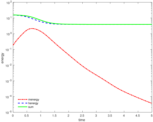
Figure 1: Plot of $\|\nabla\boldsymbol{m}_{hk}(t)\|_{{\mathbb{L}}^{2}{(D})}$ and $\|\boldsymbol{H}_{hk}(t)\|_{{\mathbb{H}}({\rm curl},D)}$ over the time.

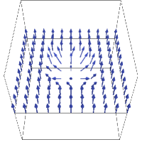
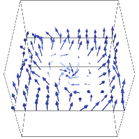
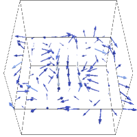
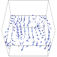
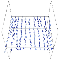
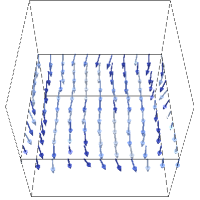
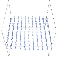
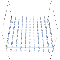
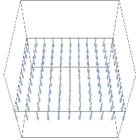
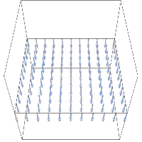
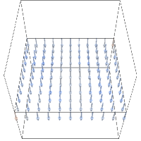
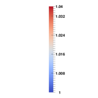
Figure 2: Slice of the magnetisation $\boldsymbol{m}_{hk}(t_{i})$ at $[0,1]^{2}\times\{1/2\}$ for $i=0,\ldots,10$ with $t_{i}=0.2i$. The colour of the vectors represents the magnitude $|\boldsymbol{m}_{hk}|$. We observe that the magnetisation aligns itself with the initial magnetic field $\boldsymbol{H}^{0}$ by performing a damped precession.

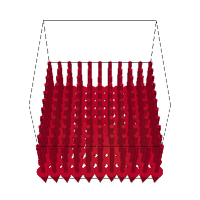
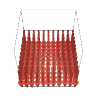
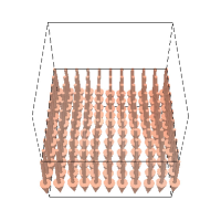
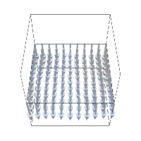
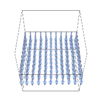
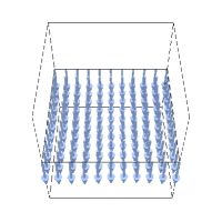
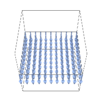
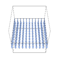
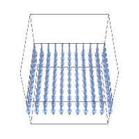
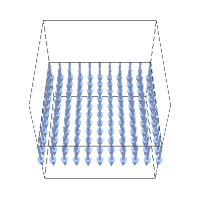
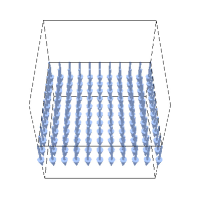
Figure 3: Slice of the magnetic field $\boldsymbol{H}_{hk}(t_{i})$ at $[0,1]^{2}\times\{1/2\}$ for $i=0,\ldots,10$ with $t_{i}=0.2i$. The colour of the vectors represents the magnitude $|\boldsymbol{H}_{hk}|$. We observe only a slight movement in the middle of the cube combined with an overall reduction of field strength.

4.2 Example 2

We use uniform time and space discretisation of the domain $D_{T}:=[0,0.1]\times D$ to partition $[0,0.1]$ into $1/k$ time intervals for $k\in\{0.001$, $0.002$, $0.004$, $0.008$, $0.016\}$ and $D$ into $\mathcal{O}(N^{3})$ tetrahedra for $N\in\{5,10,15,20,25\}$. Figure 4 shows convergence rates with respect to the space discretisation and Figure 5 with respect to the time discretization. Since the exact solution is unknown, we use the finest computed approximation as a reference solution. The convergence plots reveal that the space discretization error dominates the time discretization error by far. The expected convergence rate $\mathcal{O}(k)$ can be observed in Figure 5 which underlines the theoretical results of Theorem 2.8. It is less clear in Figure 4 if there is a convergence of order $\mathcal{O}(h)$. Preconditioners, a topic of further study, are required for implementation with larger values of $N$.

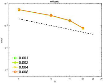
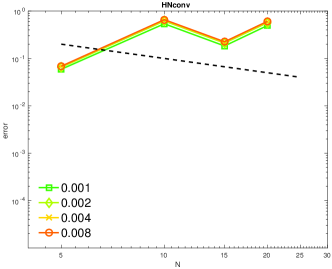
Figure 4: The convergence rate of $\|\boldsymbol{m}_{\star}-\boldsymbol{m}_{hk}\|_{L^{\infty}(0,T;H^{1}(D))}$ (left) and $\|\boldsymbol{H}_{\star}-\boldsymbol{H}_{hk}\|_{L^{2}(0,T;{\mathbb{H}}({\rm curl},D))}$ (right), where $\boldsymbol{m}_{\star}=\boldsymbol{m}_{hk}$ and $\boldsymbol{H}_{\star}=\boldsymbol{H}_{hk}$ for $h=1/25$ and $k=0.001$. The dashed line indicates $\mathcal{O}(h)$.

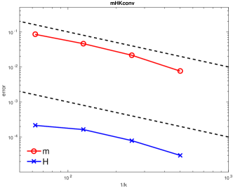
Figure 5: The convergence rate of $\|\boldsymbol{m}_{\star}-\boldsymbol{m}_{hk}\|_{L^{\infty}(0,T;H^{1}(D))}$ (red) and $\|\boldsymbol{H}_{\star}-\boldsymbol{H}_{hk}\|_{L^{2}(0,T;{\mathbb{H}}({\rm curl},D))}$ (blue), where $\boldsymbol{m}_{\star}=\boldsymbol{m}_{hk_{\star}}$ and $\boldsymbol{H}_{\star}=\boldsymbol{H}_{hk_{\star}}$ for $h=1/25$ and $k_{\star}=0.001$. The dashed lines indicate $\mathcal{O}(k)$.

Appendix

Below, we state some well-known results.

Lemma .1.

Given ${\mathcal{T}}_{h}$, there exists a constant $C_{\rm norm}>0$ which depends solely on the shape regularity of ${\mathcal{T}}_{h}$ such that

$$C_{\rm norm}^{-1}\|\nabla\boldsymbol{w}\|_{{\mathbb{L}}^{2}{(D})}\leq\Big{(}h\sum_{T\in{\mathcal{T}}_{h}}\sum_{z\in{\mathcal{N}}_{h}\cap T}|\boldsymbol{w}(z)-\boldsymbol{w}(z_{T})|^{2}\Big{)}^{1/2}\leq C_{\rm norm}\|\nabla\boldsymbol{w}\|_{{\mathbb{L}}^{2}{(D})}$$

for all $\boldsymbol{w}\in\SS^{1}({\mathcal{T}}_{h})$ and some arbitrary choice of nodes $z_{T}\in{\mathcal{N}}_{h}\cap T$ for all $T\in{\mathcal{T}}_{h}$.

Proof .2.

The proof follows from scaling arguments.

Lemma .3.

If $\{a_{i}\}$, $\{b_{i}\}$, $\{c_{i}\}$ are sequences of non-negative numbers satisfying

$$a_{i+1}\leq(1+b_{i})a_{i}+c_{i}\quad\text{for all }i\in{\mathbb{N}}_{0}$$

then for all $j\in{\mathbb{N}}_{0}$ there holds

$$a_{j}\leq\exp\big{(}\sum_{i=0}^{j-1}b_{i}\big{)}\big{(}a_{0}+\sum_{i=0}^{j-1}c_{i}\big{)}.$$

Proof .4.

The lemma can be easily shown by induction.

References

- [1] C. Abert, G. Hrkac, M. Page, D. Praetorius, M. Ruggeri, and D. Süss, Spin-polarized transport in ferromagnetic multilayers: An unconditionally convergent FEM integrator, Comput. Math. Appl., 68 (2014), pp. 639–654.
- [2] R. A. Adams, Sobolev Spaces, Academic Press [A subsidiary of Harcourt Brace Jovanovich, Publishers], New York-London, 1975. Pure and Applied Mathematics, Vol. 65.
- [3] F. Alouges, A new finite element scheme for Landau-Lifchitz equations, Discrete Contin. Dyn. Syst. Ser. S, 1 (2008), pp. 187–196, doi:10.3934/dcdss.2008.1.187.
- [4] F. Alouges, E. Kritsikis, J. Steiner, and J.-C. Toussaint, A convergent and precise finite element scheme for Landau-Lifschitz-Gilbert equation, Numer. Math., 128 (2014), pp. 407–430, doi:10.1007/s00211-014-0615-3.
- [5] F. Alouges and A. Soyeur, On global weak solutions for Landau-Lifshitz equations: existence and nonuniqueness, Nonlinear Anal., 18 (1992), pp. 1071–1084, doi:10.1016/0362-546X(92)90196-L.
- [6] M. Aurada, M. Feischl, and D. Praetorius, Convergence of some adaptive FEM-BEM coupling for elliptic but possibly nonlinear interface problems, ESAIM Math. Model. Numer. Anal., 46 (2012), pp. 1147–1173, doi:10.1051/m2an/2011075.
- [7] L. Baňas, S. Bartels, and A. Prohl, A convergent implicit finite element discretization of the Maxwell–Landau–Lifshitz–Gilbert equation, SIAM J. Numer. Anal., 46 (2008), pp. 1399–1422.
- [8] L. Baňas, M. Page, and D. Praetorius, A convergent linear finite element scheme for the Maxwell-Landau-Lifshitz-Gilbert equations, Electron. Trans. Numer. Anal., 44 (2015), pp. 250–270.
- [9] S. Bartels, Projection-free approximation of geometrically constrained partial differential equations, Math. Comp., (2015), doi:10.1090/mcom/3008.
- [10] S. Bartels, J. Ko, and A. Prohl, Numerical analysis of an explicit approximation scheme for the Landau-Lifshitz-Gilbert equation, Math. Comp., 77 (2008), pp. 773–788, doi:10.1090/S0025-5718-07-02079-0.
- [11] S. Bartels and A. Prohl, Convergence of an implicit finite element method for the Landau-Lifshitz-Gilbert equation, SIAM J. Numer. Anal., 44 (2006), pp. 1405–1419 (electronic), doi:10.1137/050631070.
- [12] J. Bergh and J. Löfström, Interpolation spaces. An introduction, Springer-Verlag, Berlin-New York, 1976. Grundlehren der Mathematischen Wissenschaften, No. 223.
- [13] A. Bossavit, Two dual formulations of the -D eddy-currents problem, COMPEL, 4 (1985), pp. 103–116, doi:10.1108/eb010005.
- [14] F. Bruckner, D. Süss, M. Feischl, T. Führer, P. Goldenits, M. Page, D. Praetorius, and M. Ruggeri, Multiscale modeling in micromagnetics: existence of solutions and numerical integration, Math. Models Methods Appl. Sci., 24 (2014), pp. 2627–2662, doi:10.1142/S0218202514500328.
- [15] A. Buffa and P. Ciarlet, Jr., On traces for functional spaces related to Maxwell’s equations. I. An integration by parts formula in Lipschitz polyhedra, Math. Methods Appl. Sci., 24 (2001), pp. 9–30, doi:10.1002/1099-1476(20010110)24:1<9::AID-MMA191>3.0.CO;2-2.
- [16] A. Buffa and P. Ciarlet, Jr., On traces for functional spaces related to Maxwell’s equations. II. Hodge decompositions on the boundary of Lipschitz polyhedra and applications, Math. Methods Appl. Sci., 24 (2001), pp. 31–48, doi:10.1002/1099-1476(20010110)24:1<9::AID-MMA191>3.0.CO;2-2.
- [17] G. Carbou and P. Fabrie, Time average in micromagnetism, J. Differential Equations, 147 (1998), pp. 383–409, doi:10.1006/jdeq.1998.3444.
- [18] I. Cimrák, Existence, regularity and local uniqueness of the solutions to the Maxwell–Landau–Lifshitz system in three dimensions, J. Math. Anal. Appl., 329 (2007), pp. 1080–1093.
- [19] I. Cimrák, A survey on the numerics and computations for the Landau-Lifshitz equation of micromagnetism, Arch. Comput. Methods Eng., 15 (2008), pp. 277–309, doi:10.1007/s11831-008-9021-2.
- [20] CTCMS, Mmmg: Micromagnetic Modeling Activity Group, http://www.ctcms.nist.gov/ rdm/mumag.org.html.
- [21] T. Gilbert, A Lagrangian formulation of the gyromagnetic equation of the magnetic field, Phys Rev, 100 (1955), pp. 1243–1255.
- [22] B. He and F. L. Teixeira, Differential forms, Galerkin duality, and sparse inverse approximations in finite element solutions of Maxwell equations, IEEE Trans. Antennas and Propagation, 55 (2007), pp. 1359–1368, doi:10.1109/TAP.2007.895619, http://dx.doi.org/10.1109/TAP.2007.895619.
- [23] M. Kružík and A. Prohl, Recent developments in the modeling, analysis, and numerics of ferromagnetism, SIAM Rev., 48 (2006), pp. 439–483, doi:10.1137/S0036144504446187.
- [24] L. Landau and E. Lifschitz, On the theory of the dispersion of magnetic permeability in ferromagnetic bodies, Phys Z Sowjetunion, 8 (1935), pp. 153–168.
- [25] K.-N. Le, M. Page, D. Praetorius, and T. Tran, On a decoupled linear FEM integrator for eddy-current-LLG, Appl. Anal., 94 (2015), pp. 1051–1067, doi:10.1080/00036811.2014.916401.
- [26] K.-N. Le and T. Tran, A convergent finite element approximation for the quasi-static Maxwell-Landau-Lifshitz-Gilbert equations, Comput. Math. Appl., 66 (2013), pp. 1389–1402, doi:10.1016/j.camwa.2013.08.009.
- [27] J. L. Lions, Quelques Méthodes de Résolution des Problèmes aux Limites Non Linéaires, Dunod Gauthier-Villars, Paris, 1969.
- [28] Automated solution of differential equations by the finite element method, vol. 84 of Lecture Notes in Computational Science and Engineering, Springer, Heidelberg, 2012, doi:10.1007/978-3-642-23099-8. The FEniCS book.
- [29] W. McLean, Strongly elliptic systems and boundary integral equations, Cambridge University Press, Cambridge, 2000.
- [30] P. Monk, Finite Element Methods for Maxwell’s equations, Numerical Mathematics and Scientific Computation, Oxford University Press, New York, 2003, doi:10.1093/acprof:oso/9780198508885.001.0001.
- [31] A. Prohl, Computational Micromagnetism, Advances in Numerical Mathematics, B. G. Teubner, Stuttgart, 2001, doi:10.1007/978-3-663-09498-2.
- [32] W. Śmigaj, T. Betcke, S. Arridge, J. Phillips, and M. Schweiger, Solving boundary integral problems with BEM++, ACM Trans. Math. Software, 41 (2015), pp. Art. 6, 40, doi:10.1145/2590830.
- [33] A. Visintin, On Landau-Lifshitz’ equations for ferromagnetism, Japan J. Appl. Math., 2 (1985), pp. 69–84, doi:10.1007/BF03167039.