Two-component generalizations of the Camassa-Holm equation

Abstract

A classification of integrable two-component systems of non-evolutionary partial differential equations that are analogous to the Camassa-Holm equation is carried out via the perturbative symmetry approach. Independently, a classification of compatible pairs of Hamiltonian operators is carried out, which leads to bi-Hamiltonian structures for the same systems of equations. Some exact solutions and Lax pairs are also constructed for the systems considered.

1 Introduction

In recent years there has been a growing interest in integrable non-evolutionary partial differential equations of the form

$$(1-D_{x}^{2})u_{t}=F(u,u_{x},u_{xx},u_{xxx},\ldots),\quad u=u(x,t),\quad D_{x}=\frac{\partial}{\partial x},$$ (1)

where $F$ is some function of $u$ and its derivatives with respect to $x$. The most celebrated example of this type of equation is the Camassa–Holm equation [1]:

$$(1-D_{x}^{2})u_{t}=3uu_{x}-2u_{x}u_{xx}-uu_{xxx}.$$ (2)

Other examples of integrable equations of the form (1) include the Degasperis-Procesi equation

$$(1-D_{x}^{2})u_{t}=4uu_{x}-3u_{x}u_{xx}-uu_{xxx},$$

(see [5, 6]) as well as equations with cubic nonlinearity, such as

$$(1-D_{x}^{2})u_{t} = u^{2}u_{xxx}+3uu_{x}u_{xx}-4u^{2}u_{x},$$

$$(1-\epsilon^{2}D_{x}^{2})u_{t} = D_{x}\left(u^{2}u_{xx}-u_{x}^{2}u_{xx}+uu_{x}^{2}-u^{3}\right)$$

(see [13, 19] and [9, 24], respectively). All the of the latter equations of Camassa-Holm type are integrable by the inverse scattering transform. They possess infinite hierarchies of local conservation laws and (quasi-)local higher symmetries, bi-Hamiltonian structures and other remarkable attributes of integrable systems. Part of the fascination with these sorts of equations is due to the fact that as well as having traditional (smooth) multi-soliton solutions, they admit weak solutions of peakon (peaked soliton) type, and also display interesting blowup and wave-breaking phenomena [14]. The complete classification of integrable equations of the form (1) was carried out in [19] using the perturbative symmetry approach introduced in [17]. Various approaches to generating multicomponent systems of Camassa-Holm type have been proposed recently, based on energy-dependent spectral problems [11], or Novikov algebras [23].

In this paper we study integrable two-component systems of the form

$$\left\{\begin{array}[]{c}(1-D_{x})u_{t}=F(u,v,u_{x},v_{x},u_{xx},v_{xx}),\\ (1+D_{x})v_{t}=G(u,v,u_{x},v_{x},u_{xx},v_{xx}),\end{array}\right.$$ (3)

where $F,G$ are polynomials over ${\mathbb{C}}$ in $u,v$ and their $x$-derivatives. An example of an integrable system of the form (3) is

$$\left\{\begin{array}[]{c}(1-D_{x})u_{t}=2(u+v)u_{x}-(u+v)u_{xx}-u_{x}^{2},\\ (1+D_{x})v_{t}=2(u+v)v_{x}+(u+v)v_{xx}+v_{x}^{2}.\end{array}\right.$$ (4)

The above system is related to a system which (up to sending $t\to-t$ and renaming variables) was given as

$$\left\{\begin{array}[]{rcl}m_{t}&=&pm_{x}+2mp_{x}-qq_{x},\\ q_{t}&=&(pq)_{x},\qquad m=(1-D_{x}^{2})p,\end{array}\right.$$ (5)

by Chen, Liu and Zhang [3], and related to an alternative system of the form (3) presented by Falqui [7], namely

$$\left\{\begin{array}[]{rcl}(1-D_{x})U_{t}&=&V_{x}+2UU_{x}-UU_{xx}-U_{x}^{2},\\ (1+D_{x})V_{t}&=&2U_{x}V+2UV_{x}+UV_{xx}+U_{x}V_{x}\end{array}\right.$$ (6)

(again, up to renaming variables, and fixing the value of a parameter). To be precise, under the transformation

$$p=u+v,\qquad q=(1-D_{x})u+(1+D_{x})v,$$ (7)

which is of Miura type, solutions of the system (4) are mapped to solutions of (5), while

$$p=U,\qquad q^{2}=\Big{(}(1-D_{x})U\Big{)}^{2}-2(1+D_{x})V$$

is a Miura map from (6) to (5).

The rest of the paper is concerned with classifying integrable systems of the form (3). In the next section we outline the perturbative symmetry approach in the context of non-evolutionary systems with two dependent variables, and explain how it leads to an integrability test for such systems. Section 3 contains the result of applying this integrability test, in the form of a list of systems with quadratic, cubic and mixed quadratic/cubic nonlinear terms; there are six systems in total, presented in Theorems 2,3 and 4 below. The fourth section is concerned with a different problem, namely that of classifying pairs of compatible Hamiltonian operators in two dependent variables. However, this turns out to be highly relevant to the preceding considerations, since it provides a bi-Hamiltonian structure for (almost) every system in the aforementioned list. In the fifth section we consider changes of independent variables, specifically reciprocal transformations (sending conservation laws to conservation laws); these are helpful for the construction of Lax pairs and exact solutions, which we illustrate in some cases. The paper ends with conclusions and suggestions for future work.

2 Integrability test: perturbative symmetries

In this section we briefly recall the basic definitions and notations of the perturbative symmetry approach (for details see [17, 18]). We also present the integrability test which we will subsequently apply to isolate integrable generalizations of the Camassa–Holm equation.

2.1 Quasi-local polynomials and definition of symmetries

Let $u,v$ be functions in $x,t$. Polynomials in $u,v$ and their $x$-derivatives over ${\mathbb{C}}$ form a differential ring ${\cal R}$ with an $x$-derivation

$$D_{x}=\sum_{k=0}^{\infty}(u_{k+1}\frac{\partial{}}{\partial{u_{k}}}+v_{k+1}\frac{\partial{}}{\partial{v_{k}}}),$$

where $u_{k},v_{k}$ denote $k$-th derivatives of $u,v$ with respect to $x$. In particular, $u_{0}$ and $v_{0}$ denote the functions $u$ and $v$ themselves. We often omit the zero index of $u_{0}$ and $v_{0}$ and simply write $u$ and $v$.

We will assume that $1\not\in{\cal R}$. Elements of the ring ${\cal R}$ are finite sums of monomials in $u,v$ and their $x$-derivatives with complex coefficients. The degree of a monomial is defined as a total power, i.e. the sum of all powers of variables that contribute to the monomial. Let ${\cal R}^{n}$ denote the set of polynomials of degree $n$ in $u,v$ and their $x$-derivatives. Then ring ${\cal R}$ has a gradation

$${\cal R}=\bigoplus_{n\in{\mathbb{Z}}_{+}}{\cal R}^{n}\,,\quad{\cal R}^{n}\cdot{\cal R}^{m}\subset{\cal R}^{n+m}\,.$$

Elements of ${\cal R}^{1}$ are linear functions of the $u,v$ and their derivatives, elements of ${\cal R}^{2}$ are quadratic, etc. It is convenient to define a “little-oh” order symbol $o({\cal R}^{n})$. We say that $f=o({\cal R}^{n})$ if $f\in\bigoplus_{k>n}{\cal R}^{k}$, i.e. the degree of every monomial of $f$ is bigger than $n$.

Since $1\not\in{\cal R}$, the kernel of the linear map $D_{x}:{\cal R}\mapsto\mbox{Im}\,D_{x}\subset{\cal R}$ is empty and therefore $D_{x}^{-1}$ is defined uniquely on $\mbox{Im}\,D_{x}$.

To an element $g\in{\cal R}$ we associate differential operators $g_{*,u}$ and $g_{*,v}$ called Fréchet derivatives with respect to $u$ and $v$ and defined as

$$g_{*,u}=\sum_{k\geq 0}\frac{\partial g}{\partial u_{k}}D_{x}^{k},\qquad g_{*,v}=\sum_{k\geq 0}\frac{\partial g}{\partial v_{k}}D_{x}^{k}.$$

Now we need to introduce a concept of quasi-local differential polynomials and the corresponding extension of the ring ${\cal R}$. The idea of this extension is similar to that in [15, 26, 17].

To rewrite the Camassa-Holm type system (3) in evolutionary form, we introduce a pair of pseudo-differential operators

$$\Delta_{-}=(1-D_{x})^{-1},\quad\Delta_{+}=(1+D_{x})^{-1}.$$ (8)

System (3) then can be rewritten as

$$\left\{\begin{array}[]{l}u_{t}=\Delta_{-}F(u,v,u_{1},v_{1},\cdots,u_{n},v_{m})\\ v_{t}=\Delta_{+}G(u,v,u_{1},v_{1},\cdots,u_{n},v_{m})\end{array}\right..$$ (11)

Clearly, if $F,G\in{\cal R}$ then the right hand side of the system (11) no longer consists of differential polynomials and we need an extension of the original differential ring ${\cal R}$.

Consider the following sequence of ring extensions:

$${\cal R}_{0}={\cal R},\quad{\cal R}_{1}=\overline{{\cal R}_{0}\bigcup\Delta_{+}({\cal R}_{0})\bigcup\Delta_{-}({\cal R}_{0})},\quad{\cal R}_{n+1}=\overline{{\cal R}_{n}\bigcup\Delta_{+}({\cal R}_{n})\bigcup\Delta_{-}({\cal R}_{n})},$$

where the set $\Delta_{\pm}({\cal R}_{n})=\{\Delta_{\pm}(a):a\in{\cal R}_{n}\}$ and the horizontal line denotes the ring closure. The index $n$ indicates the “nesting depth” of operators $\Delta_{\pm}$. We then define quasi-local differential polynomials as follows.

Definition 1.

An element $f$ is called a quasi-local differential polynomial if $f\in{\cal R}_{n}$ for sufficiently large $n$.

The right-hand side of equations in (11) lies in ${\cal R}_{1}$. Its symmetries and densities of conservation are also generally speaking all quasi-local and belong to ${\cal R}_{k}$ for some $k\geq 0$ .

We now recall the definition of a symmetry.

Definition 2.

A pair of quasi-local differential polynomials $P$ and $Q$ is called a symmetry of an evolutionary system $u_{t}=f,v_{t}=g$, where $f,g$ are quasi-local polynomials, if the system

$$u_{\tau}=P,\ v_{\tau}=Q$$

is compatible with $u_{t}=f,v_{t}=g$.

If ${\bf a}=(f,g)^{T}$ and ${\bf b}=(P,Q)^{T}$ then the above definition is equivalent to the vanishing of the Lie bracket

$$[{\bf a},{\bf b}]=\left(\begin{array}[]{cc}f_{*,u}&f_{*,v}\\ g_{*,u}&g_{*,v}\end{array}\right)\left(\begin{array}[]{l}P\\ Q\end{array}\right)-\left(\begin{array}[]{cc}P_{*,u}&P_{*,v}\\ Q_{*,u}&Q_{*,v}\end{array}\right)\left(\begin{array}[]{l}f\\ g\end{array}\right)\ .$$ (20)

We finally define a notion of formal pseudodifferential series (or just formal series) as an object of the form

$$A=\sum_{k\geq 0}a_{N-k}D_{x}^{N-k}\,,$$ (21)

with coefficients being quasi-local differential polynomials or constants. The order of the formal series (21) is $N$ (we assume that the leading coefficient $a_{N}\neq 0$). The formal series form a ring: the sum of formal series is defined in the obvious way, while multiplication (composition) is defined by

$$a_{n}D_{x}^{n}\circ b_{m}D_{x}^{m}=\sum_{k\geq 0}\left(\begin{array}[]{c}n\\ k\end{array}\right)a_{n}D_{x}^{k}(b_{m})D_{x}^{m+n-k}\,.$$ (22)

For positive $n$ the sum (22) is finite since the binomial coefficients

$$\left(\begin{array}[]{c}n\\ k\end{array}\right)=\frac{n(n-1)(n-2)\cdots(n-k+1)}{k!}$$

vanish for $k>n$, and for negative $n$ the composition is well-defined in the sense of formal series.

In the symmetry approach we admit the following definition of integrability:

Definition 3.

System (11) is integrable if it possesses an infinite hierarchy of symmetries.

In the following subsections we present the necessary conditions for existence of a hierarchy of symmetries. For this it is convenient to introduce the symbolic representation of the ring of quasi-local polynomials and derive the necessary conditions in the symbolic representation.

2.2 Symbolic representation

In this subsection we introduce the symbolic representation of the ring of differential polynomials and its extensions. We first recall the symbolic representation $\hat{\cal R}$ of the ring ${\cal R}$. A symbolic representation of a monomial

$$u_{0}^{n_{0}}u_{1}^{n_{1}}\cdots u_{p}^{n_{p}}v_{0}^{m_{0}}v_{1}^{m_{1}}\cdots v_{q}^{m_{q}},\qquad n_{0}+n_{1}+\cdots+n_{p}=n,\,m_{0}+m_{1}+\cdots+m_{q}=m$$

is defined as:

$$u_{0}^{n_{0}}u_{1}^{n_{1}}\cdots u_{p}^{n_{p}}v_{0}^{m_{0}}v_{1}^{m_{1}}\cdots v_{q}^{m_{q}}\to$$

$$\to{\hat{u}}^{n}{\hat{v}}^{m}\langle\xi_{1}^{0}\xi_{2}^{0}\cdots\xi_{n_{0}}^{0}\xi_{n_{0}+1}^{1}\cdots\xi_{n_{0}+n_{1}}^{1}\cdots\xi_{n}^{p}\rangle_{\xi}\langle\zeta_{1}^{0}\zeta_{2}^{0}\cdots\zeta_{m_{0}}^{0}\zeta_{m_{0}+1}^{1}\cdots\zeta_{m_{0}+m_{1}}^{1}\cdots\zeta_{m}^{q}\rangle_{\zeta}\ ,$$ (23)

where triangular brackets $\langle\rangle_{\xi}$ and $\langle\rangle_{\zeta}$ denote the averaging over the group $\Sigma_{n}$ of permutations of $n$ elements $\xi_{1},\ldots,\xi_{n},$ and the group $\Sigma_{m}$ of $m$ elements $\zeta_{1},\ldots,\zeta_{m}$ respectively. That is $\langle c(\xi_{1},\ldots,\xi_{n},\zeta_{1},\ldots,\zeta_{m})\rangle_{\xi}$ is

$$\langle c(\xi_{1},\ldots,\xi_{n},\zeta_{1},\ldots,\zeta_{m})\rangle_{\xi}=\frac{1}{n!}\sum_{\sigma\in\Sigma_{n}}c(\sigma(\xi_{1}),\ldots,\sigma(\xi_{n}),\zeta_{1},\ldots,\zeta_{m})$$

and the similar definition holds for averaging with respect to $\zeta$ arguments. Later we refer to this as symmetrisation operation. For example, linear monomials $u_{n},v_{m}$ are represented by

$$u_{n}\to{\hat{u}}\xi_{1}^{n},\quad v_{m}\to{\hat{v}}\zeta_{1}^{m}$$ (24)

and quadratic monomials $u_{n}u_{m}$, $u_{n}v_{m}$, $v_{n}v_{m}$ have the following symbols

$$u_{n}u_{m}\to\frac{{\hat{u}}^{2}}{2}(\xi_{1}^{n}\xi_{2}^{m}+\xi_{1}^{m}\xi_{2}^{n}),\quad u_{n}v_{m}\to{\hat{u}}{\hat{v}}(\xi_{1}^{n}\zeta_{1}^{m}),\quad v_{n}v_{m}\to\frac{{\hat{v}}^{2}}{2}(\zeta_{1}^{n}\zeta_{2}^{m}+\zeta_{1}^{m}\zeta_{2}^{n})\ .$$ (25)

To the sum of two elements of the ring corresponds the sum of their symbols. To the product of two elements $f,g\in{\cal R}$ with symbols $f\to{\hat{u}}^{n}{\hat{v}}^{m}a(\xi_{1},\ldots,\xi_{n},\zeta_{1},\ldots,\zeta_{m})$ and $g\to{\hat{u}}^{p}{\hat{v}}^{q}b(\xi_{1},\ldots,\xi_{p},\zeta_{1},\ldots,\zeta_{q})$ corresponds

$$fg\to{\hat{u}}^{n+p}{\hat{v}}^{m+q}\langle\langle a(\xi_{1},\ldots,\xi_{n},\zeta_{1},\ldots,\zeta_{m})b(\xi_{n+1},\ldots,\xi_{n+p},\zeta_{m+1},\ldots,\zeta_{m+q})\rangle_{\xi}\rangle_{\zeta},$$ (26)

where the symmetrisation operation is taken with respect to permutations of all arguments $\xi$ and $\zeta$. It is easy to see that the symbolic representations of quadratic (25) and general (23) monomials immediately follow from (24) and (26).

If $f\in{\cal R}$ has a symbol $f\to{\hat{u}}^{n}{\hat{v}}^{m}a(\xi_{1},\ldots,\xi_{n},\zeta_{1},\ldots,\zeta_{m})$, then the symbolic representation for its $N$th derivative $D_{x}^{N}(f)$ is

$$D_{x}^{N}(f)\to{\hat{u}}^{n}{\hat{v}}^{m}(\xi_{1}+\xi_{2}+\cdots+\xi_{n}+\zeta_{1}+\zeta_{2}+\cdots\zeta_{m})^{N}a(\xi_{1},\ldots,\xi_{n},\zeta_{1},\ldots,\zeta_{m}).$$

We will assign a symbol $\eta$ to the operator $D_{x}$ in the symbolic representation, with the action

$$\eta^{N}\cdot{\hat{u}}^{n}{\hat{v}}^{m}a(\xi_{1},\ldots,\xi_{n},\zeta_{1},\ldots,\zeta_{m})={\hat{u}}^{n}{\hat{v}}^{m}(\xi_{1}+\xi_{2}+\cdots+\xi_{n}+\zeta_{1}+\zeta_{2}+\cdots\zeta_{m})^{N}a(\xi_{1},\ldots,\xi_{n},\zeta_{1},\ldots,\zeta_{m})$$

If $f\in{\cal R}$ and $f\to{\hat{u}}^{n}{\hat{v}}^{m}a_{n,m}(\xi_{1},\ldots,\xi_{n},\zeta_{1},\ldots,\zeta_{m})$ then for the symbol of its Fréchet derivatives $f_{*,u}$ and $f_{*,v}$ we have

$$f_{*,u}\to n{\hat{u}}^{n-1}{\hat{v}}^{m}a_{n,m}(\xi_{1},\ldots,\xi_{n-1},\eta,\zeta_{1},\ldots,\zeta_{m}),\,f_{*,v}\to m{\hat{u}}^{n}{\hat{v}}^{m-1}a_{n,m}(\xi_{1},\ldots,\xi_{n},\zeta_{1},\ldots,\zeta_{m-1},\eta).$$

Thus we have described the symbolic representation $\hat{\cal R}$ of the differential ring ${\cal R}$.

To construct the symbolic representation of the quasi-local rings ${\cal R}_{k},\,k=1,2,\ldots$ it is enough to note that the symbolic representation of operator $\Delta_{\pm}=(1\pm D_{x})^{-1}$ is

$$\Delta_{\pm}\to(1\pm\eta)^{-1}.$$

Now if $f\in{\cal R}$ and $f\to{\hat{u}}^{n}{\hat{v}}^{m}a(\xi_{1},\ldots,\xi_{n},\zeta_{1},\ldots,\zeta_{m})$, then

$$\Delta_{\pm}(f)\to{\hat{u}}^{n}{\hat{v}}^{m}\frac{a(\xi_{1},\ldots,\xi_{n},\zeta_{1},\ldots,\zeta_{m})}{1\pm(\xi_{1}+\cdots+\xi_{n}+\zeta_{1}+\cdots+\zeta_{m})}.$$

Using the addition and multiplication operations where necessary, we thus construct the symbolic representation of $\hat{{\cal R}}_{k},\,k=1,2,\ldots$.

Finally, we define the symbolic representation for pseudo-differential formal series. For any two terms $fD_{x}^{p},\,gD_{x}^{q}$ of formal series ($p,q\in{{\mathbb{Z}}}$ and $f,g\in{\cal R}_{k}$) with symbols

$$f\to{\hat{u}}^{n}{\hat{v}}^{m}a(\xi_{1},\ldots,\xi_{n},\zeta_{1},\ldots,\zeta_{m}),\qquad g\to{\hat{u}}^{s}{\hat{v}}^{r}b(\xi_{1},\ldots,\xi_{s},\zeta_{1},\ldots,\zeta_{r})$$

the composition rule in the symbolic representation reads

$$\quad fD_{x}^{p}\circ gD_{x}^{q}\to{\hat{u}}^{n}{\hat{v}}^{m}a(\xi_{1},\ldots,\xi_{n},\zeta_{1},\ldots,\zeta_{m})\eta^{p}\circ{\hat{u}}^{s}{\hat{v}}^{r}b(\xi_{1},\ldots,\xi_{s},\zeta_{1},\ldots,\zeta_{r})\eta^{q}$$

$$={\hat{u}}^{n+s}{\hat{v}}^{m+r}\langle\langle a(\xi_{1},\ldots,\xi_{n},\zeta_{1},\ldots,\zeta_{m})(\xi_{n+1}+\cdots+\xi_{n+s}+\zeta_{m+1}+\cdots+\zeta_{m+r}+\eta)^{p}\times$$

$$\times\,b(\xi_{n+1},\ldots,\xi_{n+s},\zeta_{m+1},\ldots,\zeta_{m+r})\eta^{q}\rangle_{\xi}\rangle_{\zeta},$$ (27)

where the symmetrisation is taken with respect to permutations of arguments $\xi$ and arguments $\zeta$, but not the argument $\eta$.

More generally we consider formal series of the form

$$A=a_{00}(\eta)+{\hat{u}}a_{10}(\xi_{1},\eta)+{\hat{v}}a_{01}(\zeta_{1},\eta)+{\hat{u}}^{2}a_{20}(\xi_{1},\xi_{2},\eta)+{\hat{u}}{\hat{v}}a_{11}(\xi_{1},\zeta_{1},\eta)+{\hat{v}}^{2}a_{02}(\zeta_{1},\zeta_{2},\eta)+\cdots,$$ (28)

where the coefficients $a_{nm}(\xi_{1},\ldots,\xi_{n},\zeta_{1},\ldots,\zeta_{m},\eta)$ are formal series in $\eta$, i.e.

$$a_{nm}(\xi_{1},\ldots,\xi_{n},\zeta_{1},\ldots,\zeta_{m},\eta)=\sum_{k=k_{nm}}^{\infty}a_{nm}^{k}(\xi_{1},\ldots,\xi_{n},\zeta_{1},\ldots,\zeta_{m})\eta^{-k},$$

with $a_{nm}^{k}(\xi_{1},\ldots,\xi_{n},\zeta_{1},\ldots,\zeta_{m})$ being symmetric functions with respect to permutations of arguments $\xi_{i}$ and arguments $\zeta_{i}$. Similar to the rule (27), the composition of two monomials is defined as

$${\hat{u}}^{n}{\hat{v}}^{m}a(\xi_{1},\ldots,\xi_{n},\zeta_{1},\ldots,\zeta_{m},\eta)\circ{\hat{u}}^{p}{\hat{v}}^{q}b(\xi_{1},\ldots,\xi_{p},\zeta_{1},\ldots,\zeta_{q},\eta)$$

$$={\hat{u}}^{n+p}{\hat{v}}^{m+q}\langle\langle a(\xi_{1},\ldots,\xi_{n},\zeta_{1},\ldots,\zeta_{m},\xi_{n+1}+\cdots+\xi_{n+p}+\zeta_{m+1}+\cdots+\zeta_{m+q}+\eta)\times$$

$$\times b(\xi_{n+1},\ldots,\xi_{n+p},\zeta_{m+1},\ldots,\zeta_{m+q},\eta)\rangle_{\xi}\rangle_{\zeta}.$$

Definition 4.

We shall call a function $a_{nm}(\xi_{1},\ldots,\xi_{n},\zeta_{1},\ldots,\zeta_{m},\eta)$ quasi-local if all the coefficients of its expansion

$$a_{nm}(\xi_{1},\ldots,\xi_{n},\zeta_{1},\ldots,\zeta_{m},\eta)=\sum_{k}a_{nm}^{k}(\xi_{1},\ldots,\xi_{n},\zeta_{1},\ldots,\zeta_{m})\eta^{-k},\quad\eta\to\infty$$ (29)

are the symbolic representations of some elements from ${\cal R}_{k}$ for some $k\geq 0$.

In particular, if all the coefficients in (29) are symmetric polynomials in each of the two sets of variables $\xi_{1},\ldots,\xi_{n}$, and $\zeta_{1},\ldots,\zeta_{m}$, we say that the function $a_{nm}(\xi_{1},\ldots,\xi_{n},\zeta_{1},\ldots,\zeta_{m},\eta)$ is local.

The set of formal series (28) has the structure of an associative noncommutative ring $\hat{{\cal R}}_{\Delta}(\eta)$. It inherits the natural gradation from ${\cal R}$, namely

$$\hat{{\cal R}}_{\Delta}(\eta)=\bigoplus_{n=0}\hat{{\cal R}}_{\Delta}^{n}(\eta),$$

where $\hat{{\cal R}}_{\Delta}^{n}(\eta)$ with $n=0,1,2,3,\ldots$ are constant (i.e. independent of $u,v$ ), linear in $u$ or $v$, quadratic, cubic, etc. We say that a formal series $A=o(\hat{{\cal R}}_{\Delta}^{n}(\eta))$ if $A\in\bigoplus_{k>n}\hat{{\cal R}}_{\Delta}^{k}(\eta)$.

2.3 Formal recursion operator and necessary conditions for integrability

In this subsection we formulate the necessary conditions for integrability of a system of the form

$$\left\{\begin{array}[]{l}u_{t}=\Delta_{-}f(u,v,u_{1},v_{1},\cdots,u_{n},v_{m})\\ v_{t}=\Delta_{+}g(u,v,u_{1},v_{1},\cdots,u_{n},v_{m})\end{array}\right..$$ (32)

Let $\hat{f},\,\hat{g}$ be the symbolic representations of the differential polynomials $f,g$, so that

$$\begin{array}[]{c}\hat{f}={\hat{u}}\omega_{1}(\xi_{1})+{\hat{v}}\omega_{2}(\zeta_{1})+{\hat{u}}^{2}a_{2,0}(\xi_{1},\xi_{2})+{\hat{u}}{\hat{v}}a_{1,1}(\xi_{1},\zeta_{1})+{\hat{v}}^{2}a_{0,2}(\zeta_{1},\zeta_{2})+\cdots\\ \hat{g}={\hat{u}}\omega_{3}(\xi_{1})+{\hat{v}}\omega_{4}(\zeta_{1})+{\hat{u}}^{2}b_{2,0}(\xi_{1},\xi_{2})+{\hat{u}}{\hat{v}}b_{1,1}(\xi_{1},\zeta_{1})+{\hat{v}}^{2}b_{0,2}(\zeta_{1},\zeta_{2})+\cdots\end{array}$$ (33)

Define

$$F=\left(\begin{array}[]{cc}\hat{f}_{*,u}&\hat{f}_{*,v}\\ \hat{g}_{*,u}&\hat{g}_{*,v}\end{array}\right)$$

and let

$$\Lambda=\left(\begin{array}[]{cc}L^{(1)}&L^{(2)}\\ L^{(3)}&L^{(4)}\end{array}\right),$$ (34)

where $L^{(i)},\,i=1,\ldots,4$ are formal series,

$$L^{(i)}=\phi^{(i)}(\eta)+{\hat{u}}\phi^{(i)}_{10}(\xi_{1},\eta)+{\hat{v}}\phi^{(i)}_{01}(\zeta_{1},\eta)+{\hat{u}}^{2}\phi^{(i)}_{20}(\xi_{1},\xi_{2},\eta))+{\hat{u}}{\hat{v}}\phi^{(i)}_{11}(\xi_{1},\zeta_{1},\eta)+{\hat{v}}^{2}\phi^{(i)}_{02}(\zeta_{1},\zeta_{2},\eta)+\cdots.$$

Definition 5.

A formal series $\Lambda$ (34) is called a formal recursion operator for system (32) if all the coefficients $\phi^{(i)}_{jk}$ are quasi-local and it satisfies the equation

$$\Lambda_{t}=F\circ\Lambda-\Lambda\circ F$$ (35)

In the above definition $\Lambda_{t}$ stands for a formal series obtained from $\Lambda$ by differentiating all the coefficients $\phi_{jk}^{(i)}$ by $t$ and replacing $u_{t}$ and $v_{t}$ according to the system (32).

Theorem 1.

Assume that the system (32) is such that

$$\omega_{2}(\zeta)=0=\omega_{3}(\xi)=0$$ (36)

and $\omega_{1}(\xi)\neq c_{1}\xi,\,\,\omega_{4}(\zeta)\neq c_{4}\zeta$ (for constants $c_{1},c_{4}$). Suppose that the system (32) possesses an infinite hierarchy of quasi-local higher symmetries. Then the system possesses a formal recursion operator (34) with $\phi^{(2)}(\eta)=\phi^{(3)}(\eta)=0$ and $\phi^{(1)}(\eta)=\phi^{(4)}(\eta)=\eta$.

The assumption (36) implies that the linear part of the system (32) is diagonal; in principle, this condition may be removed. (Note that Falqui’s system (6) is excluded by this assumption.) In the diagonal case the proof of the theorem is essentially the same as the proof of the analogous Theorem 2 from [17] and therefore we omit it here.

Theorem 1 provides the necessary integrability conditions for the system (32). These can be obtained as follows:

• For a given system (32) one solves the equation (35) with respect to $\Lambda$ and finds $\phi^{(i)}_{jk}(\xi_{1},\ldots,\xi_{j},\zeta_{1},\zeta_{k},\eta)$.

• One then verifies the quasi-locality conditions of $\phi^{(i)}_{jk}(\xi_{1},\ldots,\xi_{j},\zeta_{1},\zeta_{k},\eta)$ and obtains the obstructions to integrability (if any) for the system (32).

To classify integrable systems of the Camassa-Holm type (see the next section) we only need to verify quasi-locality of $\phi^{(i)}_{jk},\,\,i=1,\ldots,4$ with $j+k\leq 3$.

3 Classification theorems

In this section we present the classification of integrable Camassa-Holm type systems of the form

$$\left\{\begin{array}[]{c}(1-D_{x})u_{t}=\lambda_{1}u_{1}+\lambda_{2}u_{2}+f\\ (1+D_{x})v_{t}=\mu_{1}v_{1}+\mu_{2}v_{2}+g\end{array}\right.,$$ (37)

where $f,g$ are polynomials containing terms of degree two or above in $u,v,u_{1},v_{1},u_{2},v_{2}$. We will also assume that $\lambda_{2}\neq-\lambda_{1}$ and $\mu_{2}\neq\mu_{1}$ as otherwise the linear part of each equation of the system will be $\lambda_{1}(1-D_{x})u_{1}$ and $\mu_{1}(1+D_{x})v_{1}$, and individually these terms are removable by a Galilean transformation.

We will restrict the classification to non-linearisable systems and therefore require the existence of non-trivial conservation laws. This allows us to further restrict the admissible linear terms in (37).

Proposition 1.

If the system (37) possesses a conservation law with nonlinear density $\rho$ then $\mu_{2}=-\lambda_{2}$ and $\mu_{1}=\lambda_{1}$.

• Rewriting the system (37) in evolutionary form and transforming the system to the symbolic representation we obtain

  $$\left\{\begin{array}[]{c}{\hat{u}}_{t}={\hat{u}}\omega_{1}(\xi_{1})+\hat{f}\\ {\hat{v}}_{t}={\hat{v}}\omega_{2}(\zeta_{1})+\hat{g}\end{array}\right.,$$ (38)

  where

  $$\omega_{1}(k)=\frac{\lambda_{1}k+\lambda_{2}k^{2}}{1-k},\quad\omega_{2}(k)=\frac{\mu_{1}k+\mu_{2}k^{2}}{1+k}$$

  and $\hat{f},\,\hat{g}$ are the symbolic representations of the $f$ and $g$. Clearly, the condition $\lambda_{2}\neq-\lambda_{1}$ and $\mu_{2}\neq\mu_{1}$ implies that $\omega_{1,2}(k)\neq c_{1,2}k$ for constants $c_{1,2}$. Assume first that $\rho$ is a density of a conservation law with symbol $\hat{\rho}={\hat{u}}^{n}{\hat{v}}^{m}a(\xi_{1},\ldots,\xi_{n},\zeta_{1},\ldots,\zeta_{m})+o(\hat{{\cal R}}^{n+m}).$ Then we must have $\rho_{t}\in\mbox{Im}(D_{x})$. In the symbolic representation we have

  $$\hat{\rho}_{t}={\hat{u}}^{n}{\hat{v}}^{m}a(\xi_{1},\ldots,\xi_{n},\zeta_{1},\ldots,\zeta_{m})\left[\omega_{1}(\xi_{1})+\cdots+\omega_{1}(\xi_{n})+\omega_{2}(\zeta_{1})+\cdots+\omega_{2}(\zeta_{m})\right]+o(\hat{{\cal R}}^{n+m}).$$

  Since $\rho_{t}\in\mbox{Im}(D_{x})$ we must have

  $$(\xi_{1}+\cdots+\xi_{n}+\zeta_{1}+\cdots+\zeta_{m})\,|\,a(\xi_{1},\ldots,\xi_{n},\zeta_{1},\ldots,\zeta_{m})\left[\omega_{1}(\xi_{1})+\cdots+\omega_{1}(\xi_{n})+\omega_{2}(\zeta_{1})+\cdots+\omega_{2}(\zeta_{m})\right]$$

  Since $\rho$ is a non-trivial density, $\rho\notin\mbox{Im}(D_{x})$ so that $a(\xi_{1},\ldots,\xi_{n},\zeta_{1},\ldots,\zeta_{m})$ is not divisible by $(\xi_{1}+\cdots+\xi_{n}+\zeta_{1}+\cdots+\zeta_{m})$, and therefore we must have

  $$(\xi_{1}+\cdots+\xi_{n}+\zeta_{1}+\cdots+\zeta_{m})\,|\,\omega_{1}(\xi_{1})+\cdots+\omega_{1}(\xi_{n})+\omega_{2}(\zeta_{1})+\cdots+\omega_{2}(\zeta_{m}).$$

  This implies

  $$\omega_{1}(\xi_{1})+\cdots+\omega_{1}(\xi_{n})+\omega_{2}(\zeta_{1})+\cdots+\omega_{2}(\zeta_{m-1})+\omega_{2}(-\xi_{1}-\cdots-\xi_{n}-\zeta_{1}-\cdots-\zeta_{m-1})=0.$$

  Assume that $n+m>2$. Then differentiating the above expression with respect to any two distinct arguments in succession we obtain either $\omega_{1}^{\prime\prime}=0$ or $\omega_{2}^{\prime\prime}=0$, which contradicts the conditions $\omega_{1,2}(k)\neq c_{1,2}k$. Clearly, if $\rho$ is a density of a non-trivial conservation law with symbol

  $$\hat{\rho}=\sum_{i=0}^{n}{\hat{u}}^{i}{\hat{v}}^{n-i}a_{i}(\xi_{1},\ldots,\xi_{i},\zeta_{1},\ldots,\zeta_{n-i})+o(\hat{{\cal R}^{n}})$$

  and $n>2$ then we again arrive at the same contradiction. So the density must necessarily start with quadratic terms, and therefore $\hat{\rho}={\hat{u}}^{2}\,a(\xi_{1},\xi_{2})+{\hat{u}}{\hat{v}}\,b(\xi_{1},\zeta_{1})+{\hat{v}}^{2}\,c(\zeta_{1},\zeta_{2})+o(\hat{{\cal R}^{2}})$. Hence

  $$\hat{\rho}_{t}={\hat{u}}^{2}\,a(\xi_{1},\xi_{2})[\omega_{1}(\xi_{1})+\omega_{1}(\xi_{2})]+{\hat{u}}{\hat{v}}\,b(\xi_{1},\zeta_{1})[\omega_{1}(\xi_{1})+\omega_{2}(\zeta_{1})]+{\hat{v}}^{2}\,c(\zeta_{1},\zeta_{2})[\omega_{2}(\zeta_{1})+\omega_{2}(\zeta_{2})]+o(\hat{{\cal R}^{2}}).$$

  Since $\rho_{t}\in\mbox{Im}{D_{x}}$ we must have

  $$a(\xi_{1},-\xi_{1})[\omega_{1}(\xi_{1})+\omega_{1}(-\xi_{1})]=0,\quad c(\zeta_{1},-\zeta_{1})[\omega_{2}(\zeta_{1})+\omega_{2}(-\zeta_{1})]=0,$$

  and $b(\xi_{1},-\xi_{1})[\omega_{1}(\xi_{1})+\omega_{2}(-\xi_{1})]=0$. If $\omega_{1}(\xi_{1})+\omega_{1}(-\xi_{1})=0$ then $\lambda_{2}=-\lambda_{1}$, which contradicts the assumptions. Thus $a(\xi_{1},-\xi_{1})=0$ and we can disregard this term as trivial. Similarly, if $\omega_{2}(\zeta_{1})+\omega_{2}(-\zeta_{1})=0$ then $\mu_{2}=\mu_{1}$, and thus we have $c(\zeta_{1},-\zeta_{1})=0$ and disregard this term as well. Therefore we must have $b(\xi_{1},-\xi_{1})\neq 0$,The last condition gives $\mu_{2}=-\lambda_{2}$ and $\mu_{1}=\lambda_{1}$. ∎

Using the above proposition with a combination of a Galilean transformation and rescaling $t$, we thus can consider only systems of the form

$$\left\{\begin{array}[]{c}(1-D_{x})u_{t}=u_{1}+f,\\ (1+D_{x})v_{t}=v_{1}+g,\end{array}\right.$$ (39)

where we assume that $f,g$ are polynomials in $u,v,u_{1},v_{1},u_{2},v_{2}$ with only quadratic terms, cubic terms, or both, and we consider these different cases separately.

Applying the integrability test as described above leads to a total of six different systems, which are listed below according to the type of nonlinearity.

Systems with quadratic nonlinearity:

Theorem 2.

If the system (39) with $f,g$ being quadratic polynomials in $u,v,u_{1},v_{1},u_{2},v_{2}$ possesses an infinite hierarchy of higher symmetries then modulo the scaling transformations $u\to\alpha u,\,v\to\beta v,\,x\to\gamma x,\,t\to\delta t$ it is one of the list

$$\left\{\begin{array}[]{l}(1-D_{x})u_{t}=u_{1}+D_{x}(2-D_{x})u^{2}+2vD_{x}(2-D_{x})u,\\ (1+D_{x})v_{t}=v_{1}+2uD_{x}(2+D_{x})v+D_{x}(2+D_{x})v^{2};\end{array}\right.$$ (40)

$$\left\{\begin{array}[]{l}(1-D_{x})u_{t}=u_{1}+D_{x}(2-D_{x})u^{2}+2D_{x}v(2-D_{x})u,\\ (1+D_{x})v_{t}=v_{1}+2D_{x}u(2+D_{x})v+D_{x}(2+D_{x})v^{2}.\end{array}\right.$$ (41)

Systems with cubic nonlinearity:

Theorem 3.

If the system (39) with $f,g$ being cubic polynomials in $u,v,u_{1},v_{1},u_{2},v_{2}$ possesses an infinite hierarchy of higher symmetries then modulo the scaling transformations $u\to\alpha u,\,v\to\beta v,\,x\to\gamma x,\,t\to\delta t$ it is one of the list

$$\left\{\begin{array}[]{l}(1-D_{x})u_{t}=u_{1}+vD_{x}(2-D_{x})u^{2},\\ (1+D_{x})v_{t}=v_{1}+uD_{x}(2+D_{x})v^{2};\end{array}\right.$$ (42)

$$\left\{\begin{array}[]{l}(1-D_{x})u_{t}=u_{1}+D_{x}v(2-D_{x})u^{2},\\ (1+D_{x})v_{t}=v_{1}+D_{x}u(2+D_{x})v^{2}.\end{array}\right.$$ (43)

Mixed nonlinearity:

Theorem 4.

If the system (39) with $f,g$ being mixed quadratic and cubic polynomials in $u,v,u_{1},v_{1},u_{2},v_{2}$ possesses an infinite hierarchy of higher symmetries then modulo the scaling transformations $u\to\alpha u,\,v\to\beta v,\,x\to\gamma x,\,t\to\delta t$ it is one of the list

$$\left\{\begin{array}[]{l}(1-D_{x})u_{t}=u_{1}+\alpha D_{x}(2-D_{x})u^{2}+2\beta D_{x}v(2-D_{x})u+\gamma D_{x}v(2-D_{x})u^{2},\\ (1+D_{x})v_{t}=v_{1}+2\alpha D_{x}u(2+D_{x})v+\beta D_{x}(2+D_{x})v^{2}+\gamma D_{x}u(2+D_{x})v^{2};\end{array}\right.$$ (44)

$$\left\{\begin{array}[]{l}(1-D_{x})u_{t}=u_{1}+\alpha D_{x}(2-D_{x})u^{2}+2\beta vD_{x}(2-D_{x})u+\gamma vD_{x}(2-D_{x})u^{2},\\ (1+D_{x})v_{t}=v_{1}+2\alpha uD_{x}(2+D_{x})v+\beta D_{x}(2+D_{x})v^{2}+\gamma uD_{x}(2+D_{x})v^{2}.\end{array}\right.$$ (45)

In the next section we consider compatible pairs of Hamiltonian operators, which will lead to bi-Hamiltonian structures for each of the six systems listed above.

4 Compatible Hamiltonian Operators

In this section, we attempt to classify integrable two-component Camassa-Holm equations based on bi-Hamiltonian structures. This is similar to the approach of [23], based on Novikov algebras; however, in due course we will obtain systems with cubic nonlinearity, which do not appear in the latter approach.

We use the multivector method, as described in the standard reference [20], to investigate the conditions such that the specified types of antisymmetric operators ${\cal H}$ with entries ${\cal H}_{ij}$, $i,j=1,2$, depending on a pair of fields $m,n$, form Hamiltonian pairs with a nondegenerate constant-coefficient differential Hamiltonian operator given by

$${\cal J}=\left(\begin{array}[]{cc}c_{1}D_{x}-c_{2}D_{x}^{3}&c_{3}D_{x}-c_{4}D_{x}^{2}\\ c_{3}D_{x}+c_{4}D_{x}^{2}&c_{5}D_{x}-c_{6}D_{x}^{3}\end{array}\right),\qquad\text{with}\,\,\text{constants}\,\,c_{i},\,i=1,\ldots,6.$$ (48)

For the purpose of deriving coupled two-component Camassa-Holm equations, we are going to study three cases:

$$({\rm i})\ c_{4}=1;\quad({\rm ii})\ c_{4}=0,c_{2}=1;\quad({\rm iii})\ c_{4}=c_{2}=0,c_{6}=1.$$ (49)

Moreover, we also use elimination requirements to get rid of non-coupled (triangular) or non-Camassa-Holm type equations by removing pairs satisfying one or more of the conditions

• $c_{1}c_{2}=c_{3}c_{4}=c_{5}c_{6}=0$;

• The determinant of ${\cal J}$ is a multiple of $D_{x}$;

• $({\cal H}_{11})_{\star,n}=({\cal H}_{12})_{\star,n}=0$ and ${\cal H}_{11}{\cal J}_{12}-{\cal H}_{12}{\cal J}_{11}=0$;

• $({\cal H}_{21})_{\star,m}=({\cal H}_{22})_{\star,m}=0$ and ${\cal H}_{21}{\cal J}_{22}-{\cal H}_{22}{\cal J}_{21}=0$.

Otherwise, we refer to the Hamiltonian pairs ${\cal H}$ and ${\cal J}$ as non-trivial CH Hamiltonian pairs.

4.1 Compatible linear Hamiltonian operators

We consider linear antisymmetric differential operators in dependent variables ${m}$, ${n}$, of the form

$${\cal H}=\left(\begin{array}[]{cc}a_{1}({m}D_{x}+D_{x}{m})+a_{2}({n}D_{x}+D_{x}{n})&a_{3}{m}D_{x}+a_{4}{m}_{1}+a_{5}{n}D_{x}+a_{6}{n}_{1}\\ a_{3}D_{x}{m}-a_{4}{m}_{1}+a_{5}D_{x}{n}-a_{6}{n}_{1}&a_{7}({m}D_{x}+D_{x}{m})+a_{8}({n}D_{x}+D_{x}{n})\end{array}\right),$$ (52)

where $a_{i},i=1,\ldots,8$ are constants.

Theorem 5.

Let the operators ${\cal H}$ and ${\cal J}$ be given by (52) and (48), respectively.

• Suppose that $c_{4}=1$. There are three non-trivial CH Hamiltonian pairs:

  1. ${\cal H}^{(1)}\!=\!\left(\!\!\!\begin{array}[]{cc}a_{1}({m}D_{x}+D_{x}{m})&a_{1}{n}D_{x}\\ a_{1}D_{x}{n}&0\end{array}\!\!\!\right),\ {\cal J}^{(1)}=\left(\!\!\!\begin{array}[]{cc}c_{1}D_{x}-c_{2}D_{x}^{3}&c_{3}D_{x}-D_{x}^{2}\\ c_{3}D_{x}+D_{x}^{2}&c_{5}D_{x}\end{array}\!\!\!\right),\ a_{1}c_{2}\neq 0;$

  2. ${\cal H}^{(2)}\!=\!\left(\!\!\!\begin{array}[]{cc}0&a_{8}D_{x}{m}\\ a_{8}{m}D_{x}&a_{8}({n}D_{x}+D_{x}{n})\end{array}\!\!\!\right),\ {\cal J}^{(2)}\!=\!\left(\!\!\!\begin{array}[]{cc}c_{1}D_{x}&c_{3}D_{x}-D_{x}^{2}\\ c_{3}D_{x}+D_{x}^{2}&c_{5}D_{x}-c_{6}D_{x}^{3}\end{array}\!\!\!\right),\ a_{8}c_{6}\neq 0;$

  3. ${\cal H}^{(3)}\!\!=\!\!\left(\!\!\!\!\begin{array}[]{cc}a_{1}({m}D_{x}+D_{x}{m})\!&\!a_{1}{n}D_{x}+a_{8}D_{x}{m}\\ a_{1}D_{x}{n}+a_{8}{m}D_{x}\!&\!a_{8}({n}D_{x}+D_{x}{n})\end{array}\!\!\!\right)\!,\ {\cal J}^{(3)}\!\!=\!\!\left(\!\!\!\!\begin{array}[]{cc}c_{1}D_{x}\!&\!c_{3}D_{x}-D_{x}^{2}\\ c_{3}D_{x}+D_{x}^{2}\!&\!c_{5}D_{x}\end{array}\!\!\!\right)\!,$ $a_{1}a_{8}\neq 0$.

• Suppose that $c_{4}=0$, $c_{2}=1$ and the parameter $c_{3}$ is arbitrary.There are two non-trivial CH Hamiltonian pairs:

  1. ${\cal H}^{(4)}\!=\!\left(\!\!\begin{array}[]{cc}a_{1}({m}D_{x}+D_{x}{m})+a_{2}({n}D_{x}+D_{x}{n})&a_{2}c_{6}({m}D_{x}+D_{x}{m})+a_{6}({n}D_{x}+D_{x}{n})\\ a_{2}c_{6}({m}D_{x}+D_{x}{m})+a_{6}({n}D_{x}+D_{x}{n})&a_{6}c_{6}({m}D_{x}+D_{x}{m})+a_{8}({n}D_{x}+D_{x}{n})\end{array}\!\!\right),\\ {\cal J}^{(4)}\!\!=\!\!\left(\!\!\begin{array}[]{cc}c_{1}D_{x}\!-\!D_{x}^{3}&0\\ 0&\!\!\!\!\!\!c_{1}c_{6}D_{x}\!-\!c_{6}D_{x}^{3}\end{array}\right),\qquad a_{1}a_{6}-a_{2}^{2}c_{6}+a_{2}a_{8}-a_{6}^{2}=0\ \mbox{and}\ c_{6}\neq 0;$

  2. ${\cal H}^{(5)}\!=\!\left(\!\!\!\begin{array}[]{cc}a_{1}({m}D_{x}+D_{x}{m})&a_{1}{n}D_{x}\\ a_{1}D_{x}{n}&0\end{array}\!\!\!\right),\ {\cal J}^{(5)}\!=\!\left(\!\!\!\begin{array}[]{cc}c_{1}D_{x}-D_{x}^{3}&c_{3}D_{x}\\ c_{3}D_{x}&c_{5}D_{x}\end{array}\!\!\!\right),\ a_{1}c_{5}\neq 0.$

• Suppose that $c_{4}=c_{2}=0$, $c_{6}=1$ and the parameter $c_{3}$ is arbitrary. There is only one non-trivial CH Hamiltonian pair:

  1. ${\cal H}^{(6)}=\left(\!\!\!\begin{array}[]{cc}0&a_{8}D_{x}{m}\\ a_{8}{m}D_{x}&a_{8}({n}D_{x}+D_{x}{n})\end{array}\!\!\!\right),\ {\cal J}^{(6)}=\left(\!\!\!\begin{array}[]{cc}c_{1}D_{x}&c_{3}D_{x}\\ c_{3}D_{x}&c_{5}D_{x}-D_{x}^{3}\end{array}\!\!\!\right),\quad a_{8}c_{1}\neq 0.$

• For the operators (48) and (52), acting on the univector $\bf\xi$, we have

  $${\cal J}({\bf\xi})\!=\!{\cal J}\left(\!\!\!\begin{array}[]{c}\theta\\ \eta\end{array}\!\!\!\right)\!=\!\left(\!\!\!\begin{array}[]{c}c_{1}\theta_{1}-c_{2}\theta_{3}+c_{3}\eta_{1}-c_{4}\eta_{2}\\ c_{3}\theta_{1}+c_{4}\theta_{2}+c_{5}\eta_{1}-c_{6}\eta_{3}\end{array}\!\!\!\right);$$ (57)

  $${\cal H}({\bf\xi})\!=\!{\cal H}\left(\!\!\!\begin{array}[]{c}\theta\\ \eta\end{array}\!\!\!\right)\!=\!\left(\!\!\!\begin{array}[]{c}P\\ Q\end{array}\!\!\!\right)$$ (62)

  $$\!=\!\left(\!\!\!\begin{array}[]{c}2a_{1}{m}\theta_{1}+a_{1}{m}_{1}\theta+2a_{2}{n}\theta_{1}+a_{2}{n}_{1}\theta+a_{3}{m}\eta_{1}+a_{4}{m}_{1}\eta+a_{5}{n}\eta_{1}+a_{6}{n}_{1}\eta\\ a_{3}{m}\theta_{1}\!+\!(a_{3}\!-\!a_{4}){m}_{1}\theta\!+\!a_{5}{n}\theta_{1}\!+\!(a_{5}\!-\!a_{6}){n}_{1}\theta\!+\!2a_{7}{m}\eta_{1}\!+\!a_{7}{m}_{1}\eta\!+\!2a_{8}{n}\eta_{1}\!+\!a_{8}{n}_{1}\eta\end{array}\!\!\!\right)\!\!,$$ (65)

  where we used the notation $D_{x}^{i}\theta=\theta_{i}$ and $D_{x}^{i}\eta=\eta_{i}$. We define the bivector associated to the operator ${\cal H}$ by

  $$\Theta_{{\cal H}}=\frac{1}{2}\int{\bf\xi}\wedge{\cal H}({\bf\xi}) = \!\!\!\int\!\!(a_{1}{m}+a_{2}{n})\theta\wedge\theta_{1}\!+\!\Big{(}(a_{3}-a_{4}){m}+(a_{5}-a_{6}){n}\Big{)}\theta\wedge\eta_{1}\!$$

  $$\!\!-\!(a_{4}{m}+a_{6}{n})\theta_{1}\wedge\eta\!+\!(a_{7}{m}+a_{8}{n})\eta\wedge\eta_{1},$$

  where $\int f=\int g$ denotes the equivalence relation $f\equiv g$ iff $f-g\in{\rm Im}D_{x}$. The operator ${\cal H}$ is Hamiltonian if and only if it satisfies the Jacobi identity, which is equivalent [20] to the vanishing of the trivector

  $${\rm Pr}_{{\cal H}({\bf\xi})}(\Theta_{{\cal H}})\!\!=\!\!\!\int\!\!\{(a_{1}P+a_{2}Q)\wedge\theta\wedge\theta_{1}\!+\!(a_{3}-a_{4})P\wedge\theta\wedge\eta_{1}\!\}$$

  $$+\int\!\!\{(a_{5}-a_{6})Q\wedge\theta\wedge\eta_{1}-\!(a_{4}P+a_{6}Q)\wedge\theta_{1}\wedge\eta\!+\!(a_{7}P+a_{8}Q)\wedge\eta\wedge\eta_{1}\},$$ (66)

  where $P$ and $Q$ are given by (65). We substitute them into it and simplify the expression, which leads to an algebraic system for the constants $a_{j},j=1,\ldots,8$, that is

  $$\left\{\!\!\begin{array}[]{l}a_{1}a_{5}+2a_{2}a_{8}-2a_{2}a_{3}+2a_{2}a_{4}-a_{5}^{2}+a_{5}a_{6}=0;\quad a_{2}a_{7}-a_{3}a_{6}+a_{4}a_{6}=0;\\ 2a_{2}a_{7}-a_{1}a_{3}+2a_{1}a_{4}-a_{3}a_{5}+a_{3}a_{6}=0;\ \ 2a_{1}a_{7}+a_{3}a_{8}-a_{3}a_{4}-2a_{6}a_{7}=0;\\ a_{1}a_{6}+a_{2}a_{8}-a_{5}a_{6}+a_{6}^{2}-a_{2}a_{4}=0;\quad 2a_{2}a_{7}+a_{5}a_{8}-a_{4}a_{5}-2a_{6}a_{8}=0;\\ a_{1}a_{7}+a_{3}a_{8}-a_{4}a_{8}-a_{3}a_{4}+a_{4}^{2}-a_{5}a_{7}+a_{6}a_{7}=0;\quad a_{2}a_{7}-a_{3}a_{6}+a_{4}a_{6}=0.\end{array}\right.$$ (71)

  The system (71) provides necessary and sufficient conditions for ${\cal H}$ to be Hamiltonian. For the purposes of this theorem, we solve it together with the conditions for ${\cal H}$ to be compatible with the constant Hamiltonian operator ${\cal J}$, that is, the trivector ${\rm Pr}_{{\cal J}({\bf\xi})}(\Theta_{{\cal H}})$ vanishes [20]. We carry out this calculation in the same way as for (66) and obtain an algebraic system for the constants $c_{i},a_{j}$, for $i=1,\ldots,6$, $j=1,\ldots,8$, namely

  $$\left\{\begin{array}[]{l}a_{2}c_{4}=0;\ a_{7}c_{4}=0;\ a_{6}c_{4}=0;\ a_{1}c_{3}+a_{2}c_{5}-a_{3}c_{1}+a_{4}c_{1}-a_{5}c_{3}+a_{6}c_{3}=0;\\ a_{5}c_{4}-a_{6}c_{4}-a_{1}c_{4}=0;\ -a_{2}c_{6}+a_{3}c_{2}-a_{4}c_{2}=0;\ a_{3}c_{2}-2a_{4}c_{2}=0;\ a_{3}c_{4}-a_{4}c_{4}=0;\\ (a_{8}-a_{4})c_{4}=0;\ -a_{5}c_{6}+2a_{6}c_{6}=0;\ a_{7}c_{1}+a_{8}c_{3}-a_{4}c_{3}-a_{6}c_{5}=0;\ -a_{7}c_{2}+a_{6}c_{6}=0.\end{array}\right.$$ (75)

  Upon solving the latter system together with (71), when $c_{4}=1$ we get the following three solutions after applying our elimination requirements:

  1. $a_{5}=a_{1},\ a_{2}=a_{3}=a_{4}=a_{6}=a_{7}=a_{8}=c_{6}=0,\ a_{1}c_{2}\neq 0;$

  2. $a_{3}=a_{4}=a_{8},\ a_{1}=a_{2}=a_{5}=a_{6}=a_{7}=c_{2}=0,\ a_{8}c_{6}\neq 0;$

  3. $a_{5}=a_{1},\ a_{3}=a_{4}=a_{8},\ a_{2}=a_{6}=a_{7}=c_{2}=c_{6}=0,\ a_{1}a_{8}\neq 0$;

  these correspond to the three nontrivial CH Hamiltonian pairs (i)-(iii) in the statement. Similarly, we treat the other two cases with the help of the Maple package Gröebner and obtained the listed pairs (iv)-(vi). This completes the proof. ∎

Any compatible Hamiltonian pair ${\cal H}$ and ${\cal J}$ which does not depend explicitly on the independent variables $x$ and $t$, with ${\cal J}$ nondegenerate, leads to an integrable equation for the vector of dependent variables ${\bf m}$, that is

$${\bf m}_{t}={\cal H}{\cal J}^{-1}({\bf m}_{x}).$$ (76)

In fact, for scalar ${\bf m}$, the Camassa-Holm equation (2) was first constructed in this way in [8] (although the correct form of the equation itself did not appear until [1]). In the case at hand, with the vector ${\bf m}=\left({m},{n}\right)^{T}$, we apply this construction to the compatible Hamiltonian pairs listed in Theorem 5. Since the pairs of operators ${\cal J}^{(i)},{\cal H}^{(i)}$ for $i=1,\ldots,6$ in the six cases above depend linearly on arbitrary constant parameters, in each case we have a lot of freedom to obtain different compatible pairs, by fixing the constants in the operator ${\cal J}^{(i)}$ to get ${\cal J}$, and taking linear combinations of ${\cal J}^{(i)}$ and ${\cal H}^{(i)}$ with different constants to get ${\cal H}$.

From case (i), we get the integrable equation

$$\left(\begin{array}[]{c}{m}_{t}\\ {n}_{t}\end{array}\right)=\left({\cal H}^{(1)}+\left(\begin{array}[]{cc}c_{1}D_{x}-c_{2}D_{x}^{3}&c_{3}D_{x}\\ c_{3}D_{x}&\!\!\!\!c_{5}D_{x}\end{array}\right)\right)\left(\begin{array}[]{cc}0&\!\!\!\!\!D_{x}-D_{x}^{2}\\ D_{x}+D_{x}^{2}&0\end{array}\right)^{-1}\left(\begin{array}[]{c}{m}_{x}\\ {n}_{x}\end{array}\right).$$

Letting

$${m}=(1-D_{x}){u},\quad{n}=(1+D_{x}){v},$$ (78)

it follows that

$$\left\{\begin{array}[]{l}(1-D_{x}){u}_{t}=a_{1}D_{x}{v}(2-D_{x}){u}+c_{3}{u}_{x}+c_{1}{v}_{x}-c_{2}{v}_{xxx}\\ (1+D_{x}){v}_{t}=\frac{a_{1}}{2}D_{x}(2+D_{x}){v}^{2}+c_{3}{v}_{x}+c_{5}{u}_{x}\end{array}\right.\qquad(a_{1}c_{2}\neq 0).$$ (81)

In the same way, from cases (ii) and (iii) we get two pairs of integrable equations, given by

$$\left\{\begin{array}[]{l}(1-D_{x}){u}_{t}=\frac{a_{8}}{2}D_{x}(2-D_{x}){u}^{2}+c_{3}{u}_{x}+c_{1}{v}_{x}\\ (1+D_{x}){v}_{t}=a_{8}D_{x}{u}(2+D_{x}){v}+c_{3}{v}_{x}+c_{5}{u}_{x}-c_{6}{u}_{xxx}\end{array}\right.\qquad(a_{8}c_{6}\neq 0),$$ (84)

$$\left\{\begin{array}[]{l}(1-D_{x}){u}_{t}=a_{1}D_{x}{v}(2-D_{x}){u}+\frac{a_{8}}{2}D_{x}(2-D_{x}){u}^{2}+c_{3}{u}_{x}+c_{1}{v}_{x}\\ (1+D_{x}){v}_{t}=\frac{a_{1}}{2}D_{x}(2+D_{x}){v}^{2}+a_{8}D_{x}{u}(2+D_{x}){v}+c_{3}{v}_{x}+c_{5}{u}_{x}\end{array}\right.\ (a_{1}a_{8}\neq 0),$$ (87)

respectively. Notice that system (84) is the same as (81), upon swapping dependent variables ${u}\leftrightarrow{v}$ and sending $x\to-x$; they do not belong in the list in the previous section since they include third derivatives, putting them outside the family (37). In fact, the system (81) can be seen to be a reduction of Example 2 on p.97 of [23] by setting the parameters $h=0$, $f=1$ and performing a Galilean transformation. It is also worth pointing out that it is possible to relax our elimination conditions slightly and still obtain interesting bi-Hamiltonian systems; for instance, setting $c_{3}=c_{5}=c_{6}=0$ in (84) or $a_{1}=c_{3}=c_{5}=0$ in (87), with $a_{8}=c_{1}=1$ in both cases, gives Falqui’s system (6), which is almost triangular (it would be with $c_{1}=0$).

For the system (87), if we take $c_{1}=c_{5}=0$ and $c_{3}=1$ and rescale ${u}$ and ${v}$, we get the system (41) in Theorem 2. Thus we arrive at the following result:

Corollary 1.

Define ${m}$ and ${n}$ as in (78). System (41) is bi-Hamiltonian, having the form

$${\bf m}_{t}={\cal H}_{1}\delta\rho_{2}={\cal H}_{2}\delta\rho_{1},$$

where the compatible Hamiltonian operators ${\cal H}_{1}$ and ${\cal H}_{2}$ are given by

$${\cal H}_{1}\!\!=\!\!\left(\!\!\begin{array}[]{cc}0\!&\!D_{x}-D_{x}^{2}\\ D_{x}+D_{x}^{2}\!&\!0\end{array}\!\!\right),\quad{\cal H}_{2}\!\!=\!\!\left(\!\!\begin{array}[]{cc}2{m}D_{x}+2D_{x}{m}\!&\!2{n}D_{x}+2D_{x}{m}+D_{x}\\ 2D_{x}{n}+2{m}D_{x}+D_{x}\!&\!2{n}D_{x}+2D_{x}{n}\end{array}\!\!\right)$$

and the corresponding Hamiltonian functions are given by the densities $\rho_{1}={u}{n}$ and $\rho_{2}={u}{v}(2{m}+2{n}+1)$.

Remark 1.

To fix the notation, note that for the Hamiltonian $H=H[{\bf m}]=\int\rho\,\mathrm{d}x$ defined by the density $\rho$, we write the variational derivative as

$$\delta\rho=\frac{\delta H}{\delta{\bf m}}=\left(\frac{\delta H}{\delta m},\frac{\delta H}{\delta n}\right)^{T},$$

in the two-component case at hand. Also, recall that when $\rho$ (and hence $H$) is specified in terms of Miura-related variables ${\bf u}$, with the Miura map ${\bf m}={\cal M}({\bf u})$, the chain rule is

$$\frac{\delta H}{\delta{\bf u}}={\cal M}_{*}({\bf u})^{\dagger}\frac{\delta H}{\delta{\bf m}},$$

where the star denotes the Fr’echet derivative, and the dagger denotes the adjoint operator.

Remark 2.

Upon taking the linear combinations $\hat{u}=\frac{1}{2}(u-v)$, $\hat{v}=\frac{1}{2i}(u+v)$ and applying a Galilean transformation together with suitable rescalings, the system (41) can be seen to be equivalent to Example 1 on p.97 of [23] with parameters $h=\beta=0$.

For case (iv), if we let

$${m}=(1-D_{x}^{2}){u};\quad{n}=(1-D_{x}^{2}){v},$$ (89)

then we obtain the integrable equation

$$\left(\begin{array}[]{c}{m}_{t}\\ {n}_{t}\end{array}\right)=\left({\cal H}^{(4)}+\left(\begin{array}[]{cc}c_{1}D_{x}&0\\ 0&\!\!\!\!c_{1}c_{6}D_{x}\end{array}\right)\right)\left(\begin{array}[]{cc}D_{x}-D_{x}^{3}&\!\!\!\!\!0\\ 0&c_{6}(D_{x}-D_{x}^{3})\end{array}\right)^{-1}\left(\begin{array}[]{c}{m}_{x}\\ {n}_{x}\end{array}\right).$$

in the explicit form

$$\left\{\begin{array}[]{l}{m}_{t}=a_{1}(2{m}{u}_{x}+{m}_{x}{u})+a_{2}(2{n}{u}_{x}+{n}_{x}{u}+2{m}{v}_{x}+{m}_{x}{v})+\frac{a_{6}}{c_{6}}(2{n}{v}_{x}+{n}_{x}{v})+c_{1}{u}_{x}\\ {n}_{t}=a_{2}c_{6}(2{m}{u}_{x}+{m}_{x}{u})\!+\!a_{6}(2{n}{u}_{x}+{n}_{x}{u}+2{m}{v}_{x}+{m}_{x}{v})\!+\!\frac{a_{8}}{c_{6}}(2{n}{v}_{x}+{n}_{x}{v})+c_{1}{v}_{x}\\ a_{1}a_{6}-a_{2}^{2}c_{6}+a_{2}a_{8}-a_{6}^{2}=0\ \mbox{and}\ c_{6}\neq 0\end{array}\right.$$ (94)

In particular, if we take either $a_{6}=0$ or $a_{2}=0$ then we get

$$\left\{\begin{array}[]{l}{m}_{t}=a_{1}(2{m}{u}_{x}+{m}_{x}{u})+a_{2}(2{n}{u}_{x}+{n}_{x}{u}+2{m}{v}_{x}+{m}_{x}{v})\\ {n}_{t}=a_{2}c_{6}(2{m}{u}_{x}+{m}_{x}{u})+a_{2}(2{n}{v}_{x}+{n}_{x}{v})\end{array}\right.\qquad(a_{2}c_{6}\neq 0),$$ (97)

$$\left\{\begin{array}[]{l}{m}_{t}=a_{1}(2{m}{u}_{x}+{m}_{x}{u})+\frac{a_{1}}{c_{6}}(2{n}{v}_{x}+{n}_{x}{v})\\ {n}_{t}=a_{1}(2{n}{u}_{x}+{n}_{x}{u}+2{m}{v}_{x}+{m}_{x}{v})+\frac{a_{8}}{c_{6}}(2{n}{v}_{x}+{n}_{x}{v})\end{array}\right.\qquad(a_{1}c_{6}\neq 0),$$ (100)

respectively. In fact, the latter two systems are seen to be the same by swapping ${u}\leftrightarrow{v}$ and identifying parameters suitably. Taking $a_{1}=1$, $a_{8}=0$ and $c_{6}=-1$ in (100), we get the two-component CH system (26) in [25].

For case (v), we let ${m}=(1-D_{x}^{2}){u}$. Then we get the integrable system

$$\left\{\begin{array}[]{l}{m}_{t}=a_{1}(2{m}{u}_{x}+{m}_{x}{u})+\frac{a_{1}}{c_{5}}{n}{n}_{x}+\frac{c_{3}}{c_{5}}{n}_{x}+c_{1}{u}_{x}\\ {n}_{t}=c_{3}{u}_{x}+a_{1}({n}{u}_{x}+{n}_{x}{u})\end{array}\right.\qquad(a_{1}c_{5}\neq 0).$$ (103)

For case (vi), we let ${n}=(1-D_{x}^{2}){v}$. Then we get the integrable system

$$\left\{\begin{array}[]{l}{m}_{t}=c_{3}{v}_{x}+a_{8}({m}{v}_{x}+{m}_{x}{v})\\ {n}_{t}=a_{8}(2{n}{v}_{x}+{n}_{x}{v})+\frac{a_{8}}{c_{1}}{m}{m}_{x}+\frac{c_{3}}{c_{1}}{m}_{x}+c_{5}{v}_{x}\end{array}\right.\qquad(a_{8}c_{1}\neq 0).$$ (106)

Similarly to before, equations (103) and (106) are seen to be the same by swapping the dependent variables. After taking $c_{1}=0$, $c_{3}=0$ and rescaling suitably, the system (103) becomes the known two-component CH equation (5) from [3].

With a change of notation, the transformation (7) presented in the introduction is

$${u}={U}+{V},\quad{n}=(1-D_{x}){U}+(1+D_{x}){V},$$ (107)

which implies that

$$(1-D_{x}){U}=\frac{1}{2}D_{x}^{-1}({m}-(1-D_{x}){n}),\quad(1+D_{x}){V}=\frac{1}{2}D_{x}^{-1}((1+D_{x}){n}-{m}).$$ (108)

Thus equation (103) when $c_{5}=-1$, $c_{3}=1$ and $c_{1}=2$ becomes

$$\left\{\begin{array}[]{l}(1-D_{x}){U}_{t}=a_{1}(2{U}{U}_{x}-{U}{U}_{xx}-{U}_{x}^{2}+2{U}_{x}{V}-{U}_{xx}{V})+{U}_{x}\\ (1+D_{x}){V}_{t}=a_{1}(2{U}{V}_{x}+{U}{V}_{xx}+2{V}{V}_{x}+{V}{V}_{xx}+{V}_{x}^{2})+{V}_{x}\end{array}\right.\quad(a_{1}\neq 0),$$ (111)

which is system (40) when $a_{1}=2$. Thus we obtain the bi-Hamiltonian structure of system (40) by using the result for equation (103), as follows:

Corollary 2.

Define ${m}$ and ${n}$ as in (78). System (40) is a bi-Hamiltonian system, given by

$${\bf m}_{t}={\cal H}_{1}\delta\rho_{2}={\cal H}_{2}\delta\rho_{1},$$

where the compatible Hamiltonian operators ${\cal H}_{1}$ and ${\cal H}_{2}$ are given by

$${\cal H}_{1}\!\!=\!\!-\frac{1}{2}\left(\!\!\begin{array}[]{cc}0\!&\!D_{x}-1\\ D_{x}+1\!&\!0\end{array}\!\!\right),$$

$${\cal H}_{2}\!\!=\!\!\left(\!\!\begin{array}[]{cc}-D_{x}^{-1}{m}_{x}-{m}_{x}D_{x}^{-1}\!&\!{m}+{n}+\frac{1}{2}+{m}_{x}D_{x}^{-1}-D_{x}^{-1}{n}_{x}\\ -({m}+{n}+\frac{1}{2})-{n}_{x}D_{x}^{-1}+D_{x}^{-1}{m}_{x}\!&\!{n}_{x}D_{x}^{-1}+D_{x}^{-1}{n}_{x}\end{array}\!\!\right)$$

and the Hamiltonian functions are given by the densities $\rho_{1}=2{u}_{x}{n}$ and $\rho_{2}=2({v}^{2}{m}_{x}-{u}^{2}{n}_{x}-{u}^{2}{v}_{x}+{v}^{2}{u}_{x}+{u}_{x}{v})$.

• To clarify the notation, we put hats on all variables in equation (103), that is, we write $\hat{{m}},\hat{{n}}$ etc. Thus the transformation (108) becomes ${m}=\frac{1}{2}D_{x}^{-1}(\hat{{m}}-(1-D_{x})\hat{{n}})$, ${n}=\frac{1}{2}D_{x}^{-1}((1+D_{x})\hat{{n}}-\hat{{m}})$, so that

  $$\hat{{n}}={m}+{n},\quad\hat{{m}}=(1+D_{x}){m}+(1-D_{x}){n}.$$ (114)

  With $a_{1}=2$, $c_{5}=-1$, $c_{3}=1$ and $c_{1}=2$ in equation (103), the compatible Hamiltonian operators are

  $${\cal H}\!=\!\left(\!\!\!\begin{array}[]{cc}2(\hat{{m}}D_{x}+D_{x}\hat{{m}})+2D_{x}&2\hat{{n}}D_{x}+D_{x}\\ 2D_{x}\hat{{n}}+D_{x}&0\end{array}\!\!\!\right),\quad{\cal J}\!=\!\left(\!\!\!\begin{array}[]{cc}D_{x}-D_{x}^{3}&0\\ 0&-D_{x}\end{array}\!\!\!\right).$$

  Under the transformation (114), the Hamiltonian operator ${\cal J}$ is sent to

  $$\left(\!\!\!\begin{array}[]{cc}1+D_{x}&1-D_{x}\\ 1&1\end{array}\!\!\!\right)^{-1}\!\!\!{\cal J}\left(\!\!\!\begin{array}[]{cc}1-D_{x}&1\\ 1+D_{x}&1\end{array}\!\!\!\right)^{-1}\!\!\!=\frac{1}{4}\left(\!\!\!\begin{array}[]{cc}D_{x}^{-1}&1-D_{x}^{-1}\\ -D_{x}^{-1}&1+D_{x}^{-1}\end{array}\!\!\!\right)\!\!{\cal J}\left(\!\!\!\begin{array}[]{cc}-D_{x}^{-1}&D_{x}^{-1}\\ 1+D_{x}^{-1}&1-D_{x}^{-1}\end{array}\!\!\!\right)\!\!={\cal H}_{1}$$

  and ${\cal H}$ is transformed to ${\cal H}_{2}$ in the statement. ∎

Remark 3.

The inverse operator of Hamiltonian operator $2{\cal H}_{2}$ in Corollary 2 is of the form

$$\!\!\left(\!\!\begin{array}[]{cc}\frac{2{n}_{x}}{(1+2{m}+2{n})^{2}}D_{x}^{-1}+D_{x}^{-1}\frac{2{n}_{x}}{(1+2{m}+2{n})^{2}}\!&\!-\frac{1}{1+2{m}+2{n}}+\frac{2{n}_{x}}{(1+2{m}+2{n})^{2}}D_{x}^{-1}-D_{x}^{-1}\frac{2{m}_{x}}{(1+2{m}+2{n})^{2}}\\ \frac{1}{1+2{m}+2{n}}-\frac{2{m}_{x}}{(1+2{m}+2{n})^{2}}D_{x}^{-1}+D_{x}^{-1}\frac{2{n}_{x}}{(1+2{m}+2{n})^{2}}\!&\!-\frac{2{m}_{x}}{(1+2{m}+2{n})^{2}}D_{x}^{-1}-D_{x}^{-1}\frac{2{m}_{x}}{(1+2{m}+2{n})^{2}}\end{array}\!\!\right)$$

Thus the local symmetries for system (40) can be generated by the recursion operator ${\cal H}_{1}{\cal H}_{2}^{-1}$.

4.2 Compatible quadratic Hamiltonian operators

In this section, we consider antisymmetric differential operators that are quadratic in the dependent variables ${m}$ and ${n}$, instead of linear as in the previous subsection. We assume that they are of the form

$${\cal H}=\left(\begin{array}[]{cc}{\cal H}_{11}&{\cal H}_{12}\\ -{\cal H}_{12}^{\dagger}&{\cal H}_{22}\end{array}\right)+b_{14}\left(\begin{array}[]{c}{m}_{x}\\ {n}_{x}\end{array}\right)D_{x}^{-1}\left(\begin{array}[]{cc}{m}_{x}&{n}_{x}\end{array}\right),$$ (123)

where, as before, $\dagger$ denotes the adjoint operator, with

$${\cal H}_{11}=b_{1}{m}D_{x}{m}+b_{2}({m}D_{x}{n}+{n}D_{x}{m})+b_{3}{n}D_{x}{n};$$

$${\cal H}_{12}=(b_{4}{m}^{2}+b_{5}{m}{n}+b_{6}{n}^{2})D_{x}+b_{7}{m}{m}_{x}+b_{8}{m}{n}_{x}+b_{9}{m}_{x}{n}+b_{10}{n}{n}_{x};$$

$${\cal H}_{22}=b_{11}{m}D_{x}{m}+b_{12}({m}D_{x}{n}+{n}D_{x}{m})+b_{13}{n}D_{x}{n}$$

and $b_{i},i=1,\ldots,14$ being constants.

Theorem 6.

Let the operators ${\cal H}$ and ${\cal J}$ be given by (123) and (48), respectively.

• Assume that $c_{4}=1$. There is only one non-trivial CH Hamiltonian pair:

  $${\cal H}^{(c)}\!\!=\!\!b_{1}\left(\!\!\!\begin{array}[]{cc}{m}D_{x}{m}&{n}D_{x}{m}\\ {m}D_{x}{n}&{n}D_{x}{n}\!\!\!\end{array}\right)\!\!-\!\!b_{1}\left(\!\!\!\begin{array}[]{c}{m}_{x}\\ {n}_{x}\end{array}\!\!\!\right)\!\!D_{x}^{-1}\!\!\left(\!\!\!\begin{array}[]{cc}{m}_{x}&{n}_{x}\!\!\!\end{array}\right)\!=\!b_{1}D_{x}\left(\!\!\!\begin{array}[]{c}{m}\\ {n}\end{array}\!\!\!\right)\!\!D_{x}^{-1}\!\!\left(\!\!\!\begin{array}[]{cc}{m}&{n}\!\!\!\end{array}\right)D_{x},$$ (132)

  $${\cal J}^{(c)}=\left(\!\!\!\begin{array}[]{cc}c_{1}D_{x}&\!\!\!c_{3}D_{x}-D_{x}^{2}\\ c_{3}D_{x}+D_{x}^{2}&c_{5}D_{x}\end{array}\!\!\!\right),b_{1}\neq 0;$$ (135)

• Assume that $c_{4}=0$, $c_{2}=1$ or $c_{4}=c_{2}=0$, $c_{6}=1$, and the parameter $c_{3}$ is arbitrary. There are no non-trivial CH Hamiltonian pairs.

• We prove this statement in the same way as we did for Theorem 5. Due to the large degree of similarity, we avoid tedious repetition and only write down the necessary steps and results. The operator ${\cal H}$ is compatible with the Hamiltonian operator ${\cal J}$ if and only if the constants in ${\cal H}$ and ${\cal J}$ satisfy an overdetermined algebraic system of the same type as (75). When $c_{4}=1$, we solve it and obtain only one solution after applying our elimination requirements: the nonzero constants in (123) should satisfy $-b_{14}=b_{9}=b_{5}=b_{13}=b_{1}$, and $c_{2}=c_{6}=0$. We denote the operators ${\cal H}$ and ${\cal J}$ under the above constraints by ${\cal H}^{(c)}$ and ${\cal J}^{(c)}$. By direct computation, we are able to show the operator ${\cal H}^{(c)}$ is Hamiltonian, and thus we obtain the Hamiltonian pair in the statement. For other cases, there are no solutions for the above system after applying our elimination requirements. ∎

For the Hamiltonian pair given by (132) and (135) we can immediately write down the integrable two-component equation

$$\left(\begin{array}[]{c}{m}_{t}\\ {n}_{t}\end{array}\right)=\left({\cal H}^{(c)}+\left(\begin{array}[]{cc}c_{1}D_{x}&c_{3}D_{x}\\ c_{3}D_{x}&\!\!\!\!c_{5}D_{x}\end{array}\right)\right)\left(\begin{array}[]{cc}0&\!\!\!\!\!D_{x}\!-\!D_{x}^{2}\\ D_{x}\!+\!D_{x}^{2}&0\end{array}\right)^{-1}\left(\begin{array}[]{c}{m}_{x}\\ {n}_{x}\end{array}\right).$$

We introduce the same notation for ${u}$ and ${v}$ as in (78). It follows that

$$\left\{\begin{array}[]{l}(1-D_{x}){u}_{t}=\frac{b_{1}}{2}D_{x}{v}(2-D_{x}){u}^{2}+c_{3}{u}_{x}+c_{1}{v}_{x}\\ (1+D_{x}){v}_{t}=\frac{b_{1}}{2}D_{x}{u}(2+D_{x}){v}^{2}+c_{5}{u}_{x}+c_{3}{v}_{x}\end{array}\right.\qquad(b_{1}\neq 0).$$ (139)

For equation (139), if we take $c_{1}=c_{5}=0$ and $c_{3}=1$ and rescale ${u}$ and ${v}$, then we get the system (43) in Theorem 3. Thus we have the following result.

Corollary 3.

Define ${m}$ and ${n}$ as in (78). System (43) is a bi-Hamiltonian system, that is, it takes the form

$${\bf m}_{t}={\cal H}_{1}\delta\rho_{2}={\cal H}_{2}\delta\rho_{1},$$

where the compatible Hamiltonian operators ${\cal H}_{1}$ and ${\cal H}_{2}$ are given by

$${\cal H}_{1}\!\!=\!\!\left(\!\!\begin{array}[]{cc}0\!&\!D_{x}-D_{x}^{2}\\ D_{x}+D_{x}^{2}\!&\!0\end{array}\!\!\right),\quad{\cal H}_{2}\!\!=\!\!\left(\!\!\!\begin{array}[]{cc}2{m}D_{x}{m}&2{n}D_{x}{m}+D_{x}\\ 2{m}D_{x}{n}+D_{x}&2{n}D_{x}{n}\!\!\!\end{array}\right)\!\!-\!\!2\left(\!\!\!\begin{array}[]{c}{m}_{x}\\ {n}_{x}\end{array}\!\!\!\right)\!\!D_{x}^{-1}\!\!\left(\!\!\!\begin{array}[]{cc}{m}_{x}&{n}_{x}\!\!\!\end{array}\right)$$

and the corresponding Hamiltonian functions are specified by the densities $\rho_{1}={u}{n}$ and $\rho_{2}={u}^{2}{v}{n}+{u}{v}$.

Notice that we did not get system (42) in Theorem 3. This is due to the assumptions we made on the Hamiltonian operators. Indeed, it is also bi-Hamiltonian, but does not have a Hamiltonian operator of the form (123); this shows that the classification using Hamiltonian pairs is not equivalent to the symmetry approach. Here we just state the relevant result without proof, since the proof uses the same method as for Theorem 5.

Proposition 2.

Define ${m}$ and ${n}$ as in (78). System (42) is a bi-Hamiltonian system, that is,

$${\bf m}_{t}={\cal H}_{1}\delta\rho_{2}={\cal H}_{2}\delta\rho_{1},$$

where the compatible Hamiltonian operators ${\cal H}_{1}$ and ${\cal H}_{2}$ are given by

$${\cal H}_{1}\!\!=\!\!\left(\!\!\begin{array}[]{cc}0\!&\!D_{x}-1\\ D_{x}+1\!&\!0\end{array}\!\!\right),$$

$${\cal H}_{2}\!\!=\!\!\left(\!\!\!\begin{array}[]{cc}{m}D_{x}^{-1}{m}_{x}+{m}_{x}D_{x}^{-1}{m}&-{m}{n}-\frac{1}{2}+{m}D_{x}^{-1}{n}_{x}-{m}_{x}D_{x}^{-1}{n}\\ {m}{n}+\frac{1}{2}-{n}D_{x}^{-1}{m}_{x}+{n}_{x}D_{x}^{-1}{m}&-{n}D_{x}^{-1}{n}_{x}-{n}_{x}D_{x}^{-1}{n}\!\!\!\end{array}\right)$$

and the corresponding Hamiltonian densities are $\rho_{1}=2{u}{n}_{x}$ and $\rho_{2}={u}^{2}{v}{n}_{x}+{u}^{2}{v}_{x}{n}+{u}{v}_{x}$.

Remark 4.

The inverse of the Hamiltonian operator $2{\cal H}_{2}$ in Proposition 2 takes the form

$$\!\!-\left(\!\!\begin{array}[]{cc}\frac{2{n}_{x}}{(1+2{m}{n})^{2}}D_{x}^{-1}{n}+{n}D_{x}^{-1}\frac{2{n}_{x}}{(1+2{m}{n})^{2}}\!&\!-\frac{1}{1+2{m}{n}}+\frac{2{n}_{x}}{(1+2{m}{n})^{2}}D_{x}^{-1}{m}-{n}D_{x}^{-1}\frac{2{m}_{x}}{(1+2{m}{n})^{2}}\\ \frac{1}{1+2{m}{n}}-\frac{2{m}_{x}}{(1+2{m}{n})^{2}}D_{x}^{-1}{n}+{m}D_{x}^{-1}\frac{2{n}_{x}}{(1+2{m}{n})^{2}}\!&\!-\frac{2{m}_{x}}{(1+2{m}{n})^{2}}D_{x}^{-1}{m}-{m}D_{x}^{-1}\frac{2{m}_{x}}{(1+2{m}{n})^{2}}\end{array}\!\!\right)$$

Thus the local symmetries for system (42) can be generated using the recursion operator ${\cal H}_{1}{\cal H}_{2}^{-1}$.

It follows from Corollary 1 and Corollary 3 that both systems possess the same Hamiltonian operator ${\cal H}_{1}$ (in fact, ${\cal J}^{(3)}={\cal J}^{(c)}$). So both Hamiltonian operators ${\cal H}^{(3)}$ and ${\cal H}^{(c)}$ form Hamiltonian pairs with the same operator. We are able to directly verify that any linear combination of ${\cal H}^{(3)}$ and ${\cal H}^{(c)}$ is also Hamiltonian, and forms a Hamiltonian pair with ${\cal J}^{(3)}$. Thus we can construct the integrable system

$$\left\{\begin{array}[]{l}(1-D_{x}){u}_{t}=a_{1}D_{x}{v}(2-D_{x}){u}+\frac{a_{8}}{2}D_{x}(2-D_{x}){u}^{2}+\frac{b_{1}}{2}D_{x}{v}(2-D_{x}){u}^{2}+c_{3}{u}_{x}+c_{1}{v}_{x},\\ (1+D_{x}){v}_{t}=\frac{a_{1}}{2}D_{x}(2+D_{x}){v}^{2}+a_{8}D_{x}{u}(2+D_{x}){v}+\frac{b_{1}}{2}D_{x}{u}(2+D_{x}){v}^{2}+c_{5}{u}_{x}+c_{3}{v}_{x},\end{array}\right.$$ (146)

which contains both equations (87) and (139). If we take $c_{1}=c_{5}=0$, $c_{3}=1$, $a_{8}=2\alpha,a_{1}=2\beta,$ and $b_{1}=2\gamma$, then we get the system (44) in Theorem 4. Thus we have the following result.

Corollary 4.

Define ${m}$ and ${n}$ as in (78). System (44) is bi-Hamiltonian, being given by

$${\bf m}_{t}={\cal H}_{1}\delta\rho_{2}={\cal H}_{2}\delta\rho_{1},$$

where the compatible Hamiltonian operators ${\cal H}_{2}$ and ${\cal H}_{1}$ are given by

$${\cal H}_{2}\!\!=\!\!\left(\!\!\begin{array}[]{cc}2\beta({m}D_{x}+D_{x}{m})+2\gamma{m}D_{x}{m}\!&\!2\beta{n}D_{x}+2\alpha D_{x}{m}+2\gamma{n}D_{x}{m}+D_{x}\\ 2\beta D_{x}{n}+2\alpha{m}D_{x}+2\gamma{m}D_{x}{n}+D_{x}\!&\!2\alpha({n}D_{x}+D_{x}{n})+2\gamma{n}D_{x}{n}\end{array}\!\!\right)$$

$$\qquad-2\gamma\left(\!\!\!\begin{array}[]{c}{m}_{x}\\ {n}_{x}\end{array}\!\!\!\right)\!\!D_{x}^{-1}\!\!\left(\!\!\!\begin{array}[]{cc}{m}_{x}&{n}_{x}\!\!\!\end{array}\right),\qquad{\cal H}_{1}\!\!=\!\!\left(\!\!\begin{array}[]{cc}0\!&\!D_{x}-D_{x}^{2}\\ D_{x}+D_{x}^{2}\!&\!0\end{array}\!\!\right)$$

and the corresponding Hamiltonian densities are $\rho_{1}={u}{n}$ and $\rho_{2}={u}{v}(2\alpha{m}+2\beta{n}+\gamma{u}{n}+1)$.

The same situation arises for systems (40) and (42), upon comparing Corollary 2 to Proposition 2. We present the result immediately, as follows.

Corollary 5.

Define ${m}$ and ${n}$ as in (78). System (45) takes the bi-Hamiltonian form

$${\bf m}_{t}={\cal H}_{1}\delta\rho_{2}={\cal H}_{2}\delta\rho_{1},$$

where the compatible Hamiltonian operators ${\cal H}_{1}$ and ${\cal H}_{2}$ are given by

$${\cal H}_{1}\!\!=\!\!\left(\!\!\begin{array}[]{cc}0\!&\!D_{x}-1\\ D_{x}+1\!&\!0\end{array}\!\!\right),$$

$${\cal H}_{2}\!\!=\!\!\gamma\left(\!\!\!\begin{array}[]{cc}{m}D_{x}^{-1}{m}_{x}+{m}_{x}D_{x}^{-1}{m}&-{m}{n}+{m}D_{x}^{-1}{n}_{x}-{m}_{x}D_{x}^{-1}{n}\\ {m}{n}-{n}D_{x}^{-1}{m}_{x}+{n}_{x}D_{x}^{-1}{m}&-{n}D_{x}^{-1}{n}_{x}-{n}D_{x}^{-1}{n}_{x}\!\!\!\end{array}\right)$$

$$\quad+\!\!\left(\!\!\begin{array}[]{cc}\beta(D_{x}^{-1}{m}_{x}+{m}_{x}D_{x}^{-1})\!&\!-\alpha({m}+{m}_{x}D_{x}^{-1})-\beta({n}-D_{x}^{-1}{n}_{x})-\frac{1}{2}\\ \alpha({m}-D_{x}^{-1}{m}_{x})+\beta({n}+{n}_{x}D_{x}^{-1})+\frac{1}{2}\!&\!-\alpha({n}_{x}D_{x}^{-1}+D_{x}^{-1}{n}_{x})\end{array}\!\!\right)$$

and the corresponding Hamiltonian densities are $\rho_{1}=2{u}{n}_{x}$ and

$$\rho_{2}=\gamma{u}^{2}({v}{n}_{x}+{v}_{x}{n})-\beta{v}^{2}({m}_{x}+{u}_{x})+\alpha{u}^{2}({n}_{x}+{v}_{x})+{u}{v}_{x}.$$

5 Reciprocal links, Lax pairs and exact solutions

In this section we describe reciprocal transformations relating the coupled Camassa-Holm type systems to negative flows in other known integrable hierarchies. We also present Lax pairs, and provide some exact solutions in certain cases.

Before we proceed, it is worth commenting on the linear terms appearing in the systems under consideration. It is necessary to include linear dispersion terms in order to be able to apply the perturbative symmetry approach. However, given a system in the form (39), we can rescale the dependent variables and time so that $u\to\epsilon^{-1}u$, $v\to\epsilon^{-1}v$, $t\to\epsilon^{d}t$, where $d$ is the common degree of $f$ and $g$ in $u,v$ and their derivatives, and then take the limit $\epsilon\to 0$, to obtain the system in the form

$$m_{t}=\hat{f},\qquad n_{t}=\hat{g},$$

where $m=u-u_{x}$, $n=v+v_{x}$ and $\hat{f},\hat{g}$ are homogeneous of degree $d$. In general, the latter system is not isomorphic to the original system (39), although this is the case for the first quadratic system (40). Indeed, if we perform a combination of shifting the dependent variables with a Galilean transformation, that is

$$u\to u+u_{0},\qquad v\to v+v_{0},\qquad x\to x-ct,\qquad t\to t,$$ (152)

then with $u_{0}=v_{0}$ and a suitable choice of $c$ it is possible to remove the $u_{x}$ and $v_{x}$ terms on the right-hand side of (40). However, for the second quadratic system (41) this is not the case, because applying (152) creates a mixture of $u_{x}$ and $v_{x}$ terms on the right-hand side of the system; and for the systems with cubic nonlinearity, applying (152) produces additional quadratic and linear terms.

5.1 First quadratic system

We have already seen that the first quadratic system is related by a Miura map to the system (5) of Chen-Liu-Zhang. This means that we can immediately obtain a Lax pair for (40), by using the results in [3].

Proposition 3.

The first quadratic system (40) has the Lax representation

$$\begin{array}[]{rcl}\psi_{xx}&=&\left[\lambda^{2}\Big{(}2(m+n)+1\Big{)}^{2}-\lambda\Big{(}2(m+n)+1+2m_{x}-2n_{x}\Big{)}+\frac{1}{4}\right]\psi,\\ \psi_{t}&=&\,\left(\frac{1}{2\lambda}+2(u+v)+1\right)\psi_{x}-(u_{x}+v_{x})\psi,\end{array}$$

where $m=u-u_{x}$, $n=v+v_{x}$.

In fact, as already mentioned, the linear dispersion terms can be removed from this particular system without taking any scaling limit, by using (152), and after rescaling time the system becomes (4), which can be written in the form

$$m_{t}=(um)_{x}+v(m+u)_{x},\qquad n_{t}=(vn)_{x}+u(n+v)_{x}.$$

In order to obtain solutions of the system, it is helpful to make use of the second equation of the system (5), which is in conservation form, and leads to the introduction of new independent variables $X,T$ via the reciprocal transformation

$$\mathrm{d}X=q\,\mathrm{d}x+pq\,\mathrm{d}t,\quad\mathrm{d}T=\mathrm{d}t,\qquad\text{with}\quad p=u+v,\quad q=m+n.$$ (153)

As explained in [3], this change of independent variables transforms (5) to the first negative flow of the AKNS hierarchy (which, at the level of the Lax pair, is equivalent to the classical Boussinesq hierarchy, up to a gauge transformation). Under the reciprocal transformation, we have the following system of four equations relating $u,v,m,n$:

$$\begin{array}[]{rcl}m_{T}=(m+n)(m+v)u_{X},&&(m+n)u_{X}=u-m,\\ n_{T}=(m+n)(n+u)v_{X},&&(m+n)v_{X}=n-v.\end{array}$$ (154)

Solutions of this system, as functions of $X,T$, lead to parametric solutions of the original system (4). However, it turns out that it is more convenient to first obtain solutions of the second quadratic system, as described in the next subsection, and then exploit a Miura map between the two systems, rather than attempting to solve (154) directly.

5.2 Second quadratic system

In this subsection we consider the second quadratic system (41) without linear dispersion terms, which (after rescaling $t$) can be written as

$$M_{t}=\Big{(}(U+V)M+UV\Big{)}_{x},\qquad N_{t}=\Big{(}(U+V)N+UV\Big{)}_{x},$$ (155)

with $M=U-U_{x}$, $N=V+V_{x}$, where all the dependent variables are given upper case letters to distinguish them from the variables in the first quadratic system. The need to make this distinction here is due to the following result.

Proposition 4.

A solution of the first quadratic system (4) gives rise to a solution of the second quadratic system (155) via the Miura map

$$U=u+v+v_{x},\qquad V=-v_{x}$$ (156)

• From (156) it follows that $U=u+n$ and $U+V=u+v$, so that

  $$M=m+(1-D_{x})n,\qquad N=-n_{x},$$

  which gives

  $$M-N=m+n,\qquad M+N=m+n-2n_{x}.$$

  Upon taking the time derivative of the latter two equations and using (4), we see that the difference and sum of $M$ and $N$ evolve according to

  $$(M-N)_{t}=\Big{(}(U+V)(M-N)\Big{)}_{x},\qquad(M+N)_{t}=\Big{(}(U+V)(M+N)+2UV\Big{)}_{x},$$ (157)

  which is equivalent to (155). ∎

From the above, we see that the system (155) is intermediate between (4) and (5), and we can write the Miura map from (155) to (5) directly as

$$p=U+V,\qquad q=M-N.$$ (158)

By taking the Lax pair in [3], or by shifting/scaling the coefficients of the Lax pair in Proposition 3 and using (156), we immediately have the following.

Proposition 5.

The second quadratic system (155) has the Lax representation

$$\begin{array}[]{rcl}\psi_{xx}&=&\left[\lambda^{2}(M-N)^{2}-\lambda(M+N+M_{x}-N_{x})+\frac{1}{4}\right]\psi,\\ \psi_{t}&=&\,\left(\frac{1}{2\lambda}+U+V\right)\psi_{x}-\frac{1}{2}(U_{x}+V_{x})\psi,\end{array}$$

where $M=U-U_{x}$, $N=V+V_{x}$.

Next, observe that the first equation in (157) is just the conservation law $q_{t}=(pq)_{x}$. This means that the same reciprocal transformation (153) can be used to link (155) to the first negative AKNS flow. The equations (157) and the relations $M=U-U_{x}$, $N=V+V_{x}$ are transformed to

$$\begin{array}[]{rcl}(q^{-1})_{T}+p_{X}=0,&&qU_{X}=U-M,\\ \Big{(}(M+N)q^{-1}\Big{)}_{T}=(2UV)_{X},&&qV_{X}=N-V.\end{array}$$ (159)

Upon adding and subtracting the equations that involve only $X$ derivatives, and using (158), we see that the relations

$$(M+N)q^{-1}=pq^{-1}-(U-V)_{X},\qquad U-V=q(1+p_{X})$$ (160)

hold. With the introduction of a potential $f(X,T)$ into the conservation law for $q^{-1}$, such that $q^{-1}=f_{X}$, $p=-f_{T}$, it is possible to use (158) and (160) to express $U,V$ purely in terms of derivatives of $f$. Moreover, all of the terms in the conservation law for $(M+N)q^{-1}$ in (159) can also be rewritten in terms of $f$, to yield a single equation for this potential, namely

$$\left(\Big{(}\frac{f_{XT}-1}{f_{X}}\Big{)}_{X}-f_{X}f_{T}\right)_{T}=\frac{1}{2}\left(f_{T}^{2}-\frac{(f_{XT}-1)^{2}}{f_{X}^{2}}\right)_{X}.$$ (161)

The latter equation is equivalent to equation (2.16) in [3]; below we rewrite it in a form which makes it more easily identifiable as such.

Theorem 7.

Let $f(X,T)$ be a solution of the equation

$$f_{X}^{2}f_{XXTT}-f_{X}f_{XX}f_{XTT}-f_{X}f_{XT}f_{XXT}-f_{X}^{4}f_{TT}+f_{XX}f_{XT}^{2}-2f_{X}^{3}f_{T}f_{XT}-f_{XX}=0.$$

Then taking

$$U=\frac{1}{2}\Big{(}-f_{T}-(f_{XT}-1)f_{X}^{-1}\Big{)},\qquad V=\frac{1}{2}\Big{(}-f_{T}+(f_{XT}-1)f_{X}^{-1}\Big{)}$$ (162)

and

$$x=f(X,t)$$

gives a solution $(U(x,t),V(x,t))$ of the system (155) in parametric form.

Corollary 6.

A solution $(u(x,t),v(x,t))$ of the system (4) is given in parametric form by taking

$$u=\frac{1}{2}\Big{(}-X-f_{T}-\int f_{X}f_{T}\,\mathrm{d}X\Big{)},\qquad v=\frac{1}{2}\Big{(}X-f_{T}+\int f_{X}f_{T}\,\mathrm{d}X\Big{)}.$$

Proof of Corollary: Applying the reciprocal transformation (153) to the second equation in (156) yields $v_{X}=-q^{-1}V=-f_{X}V$. The expression for $v$ then follows by using the formula for $V$ in (162) and integrating with respect to $X$ (which leaves a function of time unspecified); $u$ is then found by noting that $u+v=U+V=p=-f_{T}$. ∎

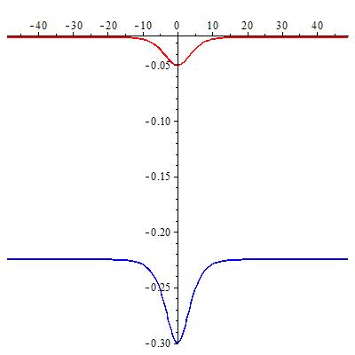
(a) Dark soliton case: $k=1/2$, $\delta=1$, $r_{0}=4$     with $c=3/4$, $\mathrm{C}=1/10$.

(b) Bright soliton case: $k=1/2$, $\delta=1$, $r_{0}=2$     with $c=9\sqrt{10}/20$, $\mathrm{C}=1/\sqrt{10}$.

Figure 1: Parametric plots of $U$ (red) and $V$ (blue) showing dark/bright solitons.

Example: travelling waves. Travelling waves of the system (155) depend on $x,t$ via the combination $z=x-ct$, where $c$ is the wave velocity. They are obtained in parametric form by taking

$$z=\hat{f}(Z),\qquad f(X,T)=\hat{f}(Z)+cT,\qquad Z=X-\mathrm{C}T,$$

which gives solutions of (161) corresponding to travelling waves with velocity $\mathrm{C}$ in the reciprocally transformed system (159). If we set $\rho=\hat{f}^{\prime}$, then (161) becomes an ordinary differential equation of third order for $\rho$, and after integrating twice this yields

$$(\rho^{\prime})^{2}=\rho^{4}-2c\mathrm{C}^{-1}\rho^{3}+K_{2}\rho^{2}+K_{1}\rho+\mathrm{C}^{-2},$$ (163)

where $K_{1},K_{2}$ are arbitrary constants. The general solution of the latter equation is an elliptic function $\rho(Z)$. In general, from (162), $U$ and $V$ are then given in parametric form in terms of $\rho(Z)$ and $\rho^{\prime}(Z)$ according to

$$U=\frac{1}{2}\left(\mathrm{C}\rho-c+\frac{\mathrm{C}\rho^{\prime}+1}{\rho}\right),\qquad V=\frac{1}{2}\left(\mathrm{C}\rho-c-\frac{\mathrm{C}\rho^{\prime}+1}{\rho}\right).$$ (164)

Here we consider single soliton solutions, which are obtained by choosing the quartic in (163) to have a double root. In that case, the solutions take the form

$$\rho(Z)=r_{0}\pm\left(\frac{2\delta k(1-k^{2})\mathrm{sinh}^{2}(\delta Z)}{1+(1-k^{2})\mathrm{sinh}^{2}(\delta Z)}\right),\qquad 0<k<1,$$ (165)

where the values of $\mathrm{C}$ and $c$ are fixed by the choice of parameters $k$ and $r_{0},\delta>0$. To be more precise, substituting the solution (165) into (163) determines $C,c,K_{1},K_{2}$, and $r_{0}$ must be chosen to ensure that $\mathrm{d}z/\mathrm{d}Z=\rho(Z)>0$ everywhere, in order for the parametric solution for $U,V$ to be single-valued. Upon integrating (165), the similarity variable $z=x-ct$ is obtained as

$$z=r_{0}Z\pm 2k\log\left(\frac{1+\mathrm{tanh}(\delta Z/2)}{1+\mathrm{tanh}(\delta Z/2)}\right)+\log\left(\frac{1\mp 2k\mathrm{tanh}(\delta Z/2)+\mathrm{tanh}^{2}(\delta Z/2)}{1\pm 2k\mathrm{tanh}(\delta Z/2)+\mathrm{tanh}^{2}(\delta Z/2)}\right),$$

up to shifting by an arbitrary constant. The field $\rho$ has the shape of a dark soliton (a wave of depression) when the plus sign is chosen in (165), while with a minus sign it is a bright soliton; in Figure 1 the corresponding fields $U,V$ given by (164) are plotted in these two different cases.

5.3 First cubic system

For simplicity, we consider the system (42) in the absence of linear terms on the right-hand sides, in which case (with suitable scaling) it can be written as

$$m_{t}=v(um)_{x},\qquad n_{t}=u(vn)_{x},\qquad\text{with}\quad m=u-u_{x},\,n=v+v_{x}.$$ (166)

In that case, it is useful to consider the first non-trivial symmetry of the system, which (up to rescaling) takes the form

$$u_{\tau}=\frac{m_{x}}{(mn)^{2}},\qquad v_{\tau}=\frac{n_{x}}{(mn)^{2}}.$$ (167)

The quantity $F=mn$ is a conserved density for both (166) and the latter symmetry, which satisfies

$$F_{t}=(uv\,F)_{x},\qquad F_{\tau}=-G_{x},\qquad\text{with}\quad F=mn,\,G=F^{-1}\Big{(}1+(\log(m/n))_{x}\Big{)}.$$ (168)

In order to find the Lax pair for the cubic system, it is helpful to consider a simultaneous reciprocal transformation in the independent variables $x,t,\tau$, by setting

$$\mathrm{d}X=F\,\mathrm{d}x+uvF\,\mathrm{d}t-G\mathrm{d}\tau,\quad\mathrm{d}T=\mathrm{d}t,\quad\mathrm{d}s=\mathrm{d}\tau.$$ (169)

(Of course, this could be extended to include the whole hierarchy of symmetries of (166), but the symmetry $\partial\tau$ is sufficient for our purposes.) The partial derivatives transform as $\partial_{x}=F\partial_{X}$, $\partial_{t}=\partial_{T}+uvF\partial_{X}$ and $\partial_{\tau}=\partial_{s}-G\partial_{X}$. To begin with, we identify the symmetry (167) by introducing new dependent variables

$$p=\frac{1}{m},\qquad q=\frac{1}{n},$$

and find that under the reciprocal transformation (169) it yields a system of derivative nonlinear Schrödinger type, namely

$$p_{s}=-p_{XX}+2qpp_{X},\qquad q_{s}=-q_{XX}+2pqq_{X},$$ (170)

which is the Chen-Lee-Liu system [2]. For the latter system, we take the Lax pair in the form

$$\begin{array}[]{l}\Psi_{X}={\bf F}\Psi,\quad\Psi_{s}={\bf G}\Psi,\qquad\text{with}\qquad{\bf F}=\left(\begin{array}[]{cc}\frac{1}{2}({\lambda}+pq)&-q\\ p{\lambda}&-\frac{1}{2}({\lambda}+pq)\end{array}\right),\\ {\bf G}=\left(\begin{array}[]{cc}\frac{1}{2}{\lambda}^{2}+pq{\lambda}+\frac{1}{2}(pq_{X}-p_{X}q+p^{2}q^{2})&-q{\lambda}-q_{X}-pq^{2}\\ p{\lambda}^{2}+(-p_{X}+p^{2}q){\lambda}&-\frac{1}{2}{\lambda}^{2}-pq{\lambda}-\frac{1}{2}(pq_{X}-p_{X}q+p^{2}q^{2})\end{array}\right).\end{array}$$ (171)

If the same reciprocal transformation (169) is applied to (166), then in terms of the variables $p,q,u,v$ we find a system given by two pairs of equations, that is

$$\begin{array}[]{rclrcl}p_{T}&=&v-puv,&q_{T}&=&-u+quv,\\ u_{X}&=&-q+upq,&v_{X}&=&p-vpq,\\ \end{array}$$ (172)

which is symmetrical under the involution

$$p\leftrightarrow-u,\qquad q\leftrightarrow-v,\qquad X\leftrightarrow-T.$$ (173)

The latter system corresponds to a negative flow in the hierarchy of symmetries of the Chen-Lee-Liu system [2], and its Lax pair is found by taking the same $X$ part as in (171) and a $T$ part which is linear in the inverse of the spectral parameter ${\lambda}$.

Proposition 6.

The system (172) has the Lax pair

$$\Psi_{X}={\bf F}\Psi,\qquad\Psi_{s}={\bf H}\Psi,$$ (174)

where ${\bf F}$ is as in (171), and

$${\bf H}=\left(\begin{array}[]{cc}\frac{1}{2}({\lambda}^{-1}+uv)&-u{\lambda}^{-1}\\ v&-\frac{1}{2}({\lambda}^{-1}+uv)\end{array}\right).$$

Remark 5.

Upon taking the first component of the vector $\Psi$ to be $\psi_{1}=\sqrt{q}\phi$, the $X$ part of the Lax pair implies that the function $\phi$ is a solution of the energy-dependent Schrödinger equation

$$\phi_{XX}=\Big{(}\frac{1}{4}{\lambda}^{2}+U{\lambda}+V\Big{)}\phi,$$

where $U,V$ are certain functions of $p,q$ and their derivatives. This shows that the system (172) is related by a Miura transformation to the first negative flow in the classical Boussinesq hierarchy.

Corollary 7.

The system (166) has the Lax pair

$$\begin{array}[]{rcl}\left(\begin{array}[]{c}\psi_{1,x}\\ \psi_{2,x}\end{array}\right)&=&\left(\begin{array}[]{cc}\frac{1}{2}(mn{\lambda}+1)&-m\\ n{\lambda}&-\frac{1}{2}(mn{\lambda}+1)\end{array}\right)\left(\begin{array}[]{c}\psi_{1}\\ \psi_{2}\end{array}\right),\\ \left(\begin{array}[]{c}\psi_{1,t}\\ \psi_{2,t}\end{array}\right)&=&\left(\begin{array}[]{cc}\frac{1}{2}(uvmn{\lambda}+2uv+{\lambda}^{-1})&-uvm-u{\lambda}^{-1}\\ uvn{\lambda}+v&-\frac{1}{2}(uvmn{\lambda}+2uv+{\lambda}^{-1})\end{array}\right)\left(\begin{array}[]{c}\psi_{1}\\ \psi_{2}\end{array}\right).\end{array}$$ (175)

Proof of Corollary: This follows immediately by applying the inverse of the reciprocal transformation (169) to the vector wave function $\Psi=(\psi_{1},\psi_{2})^{T}$ in (174). ∎

As it stands, the system (172) is not so easy to analyse from the point of view of obtaining solutions. However, the dependent variables $u,v$ can be rewritten in terms of $p,q$ and their derivatives according to the expression

$$\left(\begin{array}[]{c}u\\ v\end{array}\right)=\frac{1}{2w^{2}-w(\log r)_{X}}\left(\begin{array}[]{cc}q_{X}-qw&-q\\ p_{X}+pw&-p\end{array}\right)\left(\begin{array}[]{c}w_{T}\\ w_{XT}-2w\end{array}\right),$$ (176)

where

$$w=pq,\qquad r=\frac{q}{p}.$$

Under the reciprocal transformation (169), the conservation law for $F=w^{-1}$ becomes $w_{T}+(uv)_{X}=0$, and using (176) the product $\Pi=uv$ can be rewritten purely in terms of $w$ and $r$, leading to a system for these two variables alone, namely

$$w_{T}+\Pi_{X}=0,\qquad(\log r)_{T}=2\Pi-\frac{\cal A}{\cal B},$$ (177)

with

$$\Pi=\frac{w}{4}\left(\frac{{\cal A}^{2}}{{\cal B}^{2}}-\frac{w_{T}^{2}}{w^{2}}\right),\qquad{\cal A}=2\frac{w_{XT}}{w}-\frac{w_{X}w_{T}}{w^{2}}-4,\qquad{\cal B}=(\log r)_{X}-2w.$$

The system (177) passes the Painlevé test with expansions around a movable singularity manifold $\varphi(X,T)=0$ having the two different leading order behaviours $w\sim\pm\varphi^{-1}$, $\log r\sim\mp\log\varphi$. Moreover, from a solution of this system one recovers $p,q$, and hence also $u,v$ from (176), as functions of $X$ and $T$; via the reciprocal transformation (169), this produces a solution of (166).

Theorem 8.

Let $(f(X,T),r(X,T))$ be a solution of the system

$$\begin{array}[]{rcl}4f_{T}+f_{X}\Big{(}\hat{\cal A}^{2}\hat{\cal B}^{-2}-f_{XT}^{2}f_{X}^{-2}\Big{)}&=&0,\\ (\log r)_{T}+2f_{T}+\hat{\cal A}\hat{\cal B}^{-1}&=&0,\end{array}$$ (178)

with

$$\hat{\cal A}=2\frac{f_{XXT}}{f_{X}}-\frac{f_{XX}f_{XT}}{f_{X}^{2}}-4,\qquad\hat{\cal B}=(\log r)_{X}-2f_{X}.$$

Then taking $w(X,T)=f_{X}(X,T)$, $p=\sqrt{w/r}$, $q=\sqrt{wr}$ together with (176), and setting

$$x=f(X,t)$$

gives a solution $(u(x,t),v(x,t))$ of the system (166) in parametric form. Equivalently, a parametric solution of (166) is obtained from a solution $(f(X,T),r^{*}(X,T))$ of the system

$$\begin{array}[]{rcl}4f_{X}+f_{T}\Big{(}({\cal A}^{*})^{2}({\cal B}^{*})^{-2}-f_{XT}^{2}f_{T}^{-2}\Big{)}&=&0,\\ (\log r^{*})_{X}+2f_{X}-{\cal A}^{*}({\cal B}^{*})^{-1}&=&0,\end{array}$$ (179)

with

$${\cal A}^{*}=2\frac{f_{XTT}}{f_{T}}-\frac{f_{XT}f_{TT}}{f_{T}^{2}}-4,\qquad{\cal B}^{*}=-(\log r^{*})_{T}+2f_{T},$$

by taking $\Pi(X,T)=-f_{T}(X,T)$, $u=\sqrt{\Pi/r^{*}}$, $v=\sqrt{\Pi r^{*}}$.

• The quantity $f$ arises by introducing a potential in the first equation in (177). The differential of the above formula for $x$ gives $\mathrm{d}x=f_{X}(X,t)\,\mathrm{d}X+f_{T}(X,t)\mathrm{d}t=w\,\mathrm{d}X-\Pi\,\mathrm{d}T$, which follows by identifying $\Pi=-f_{T}$, ${\cal A}=\hat{\cal A}$ and ${\cal B}=\hat{\cal B}$, upon comparing the terms from the second equation in (177) with those in (178); this expression for $\mathrm{d}x$ corresponds precisely to the inverse of the reciprocal transformation (169), as required. The same parametric solution $(u(x,t),v(x,t))$, with $x=f(X,t)$, can be obtained in a different way by exploiting the symmetry (173). Indeed, from (172), or by applying the involution to (176), the dependent variables $p,q$ can be rewritten in terms of $u,v$ and their derivatives as

  $$\left(\begin{array}[]{c}p\\ q\end{array}\right)=\frac{1}{2\Pi^{2}+\Pi(\log r^{*})_{T}}\left(\begin{array}[]{cc}v_{T}+v\Pi&v\\ u_{T}-u\Pi&u\end{array}\right)\left(\begin{array}[]{c}\Pi_{X}\\ -\Pi_{XT}+2\Pi\end{array}\right),$$ (180)

  with $\Pi=uv$ and $r^{*}=\frac{v}{u}$. The involution (173) swaps $w\leftrightarrow\Pi$ and $r\leftrightarrow r^{*}$, and this leads to the alternative system (179), from which $u,v$ are recovered directly. ∎

Figure 2: Parametric plots of $u$ and $v$ against $z$ for (188) with $c=-3$, $\mathrm{C}=-1$, $A=1$.

Example: travelling wave solutions. To illustrate the preceding result, we consider travelling wave solutions of (166), such that $u$ and $v$ are functions of $z=x-ct$, where $c$ is the velocity of the waves. By comparing the conservation law (168), or the first equation in (177), with the reciprocal transformation (169) (where we ignore $\mathrm{d}\tau$ and $\mathrm{d}s$), it follows that such solutions correspond to travelling waves in the system (172) which are functions of the variable $Z=X-\mathrm{C}T$ for another constant $\mathrm{C}$, where setting $pq=w(X,T)\to w(Z)$, $uv=\Pi(X,T)\to\pi(Z)$ yields

$$\mathrm{C}w=\pi+c.$$ (181)

Furthermore, for the independent variables we have

$$\mathrm{d}z=\mathrm{d}x-c\mathrm{d}t=w(X,T)\,\mathrm{d}X-\Pi(X,T)\,\mathrm{d}T-c\,\mathrm{d}t=w(Z)\,\mathrm{d}X-(\pi(Z)+c)\mathrm{d}T=w(Z)\,\mathrm{d}Z,$$

by (181). so if we replace $f(X,T)\to\tilde{f}(Z)+cT$ then

$$z=\tilde{f}(Z),\qquad\text{with}\quad\tilde{f}^{\prime}(Z)=w(Z)=\mathrm{C}^{-1}(\pi(Z)+c),$$ (182)

where the prime denotes $\mathrm{d}/\mathrm{d}Z$. To describe these travelling waves, it is most convenient to obtain a single equation for $\pi(Z)$, which is achieved by first using the definition of ${\cal B}^{*}$ to write

$$(\log r^{*})^{\prime}=\mathrm{C}^{-1}({\cal B}^{*}+2\pi),$$ (183)

then putting this and (181) into (179), to obtain a pair of quadratic equations in ${\cal B}^{*}$ with coefficients depending only on $\pi$ and its derivatives. After eliminating ${\cal B}^{*}$ to find

$${\cal B}^{*}=-\frac{\mathrm{C}\Big{(}2\mathrm{C}\pi\pi^{\prime\prime}-\mathrm{C}(\pi^{\prime})^{2}+4\pi^{2}\Big{)}\Big{(}\mathrm{C}\pi^{\prime\prime}+4\pi+2c\Big{)}}{\pi(2\pi+c)\Big{(}\mathrm{C}(\pi^{\prime})^{2}+4\pi^{2}+4c\pi\Big{)}},$$ (184)

then removing a prefactor, a single equation of second order and second degree for $\pi$ results:

$$\Big{(}\pi^{\prime\prime}+\mathrm{C}^{-1}(4\pi+2c)\Big{)}^{2}=\mathrm{C}^{-2}\Big{(}4\pi^{2}+4c\pi+c^{2}\Big{)}(\pi^{\prime})^{2}+\mathrm{C}^{-3}\Big{(}16\pi^{4}+32c\pi^{3}+20c^{2}\pi^{2}+4c^{3}\pi\Big{)}.$$ (185)

The latter equation has a first integral: if $\pi$ satisfies the first order equation

$$(\pi^{\prime})^{2}=\frac{\pi^{4}}{\mathrm{C}^{2}}+\frac{2c\pi^{3}}{\mathrm{C}^{2}}+\left(\frac{c^{2}}{\mathrm{C}^{2}}-4K\right)\pi^{2}-4Kc\pi+4(K\mathrm{C}-1)^{2}\equiv\mathrm{Q}(\pi),$$ (186)

for any constant value $K$, then it satisfies (185). The generic solution of (186) is an elliptic function of $Z$, but to have bounded periodic solutions for real $c,\mathrm{C},K$ requires that the curve $(\pi^{\prime})^{2}=\mathrm{Q}(\pi)$ in the real $(\pi,\pi^{\prime})$ phase plane should have a compact component (see Figure 3(a)), otherwise solutions are generically unbounded with simple poles on the real $Z$ axis.

(a) The quartic curve (186) in the $(\pi,\pi^{\prime})$ plane.

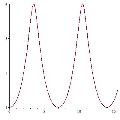
(b) Parametric plot of $(z(Z),\pi(Z)$).

Figure 3: Phase plane and $\pi$ against $z$ in the case $c=-5$, $\mathrm{C}=-1$, $K=-1$.

The quartic $\mathrm{Q}$ has discriminant $\Delta=256(2K\mathrm{C}-1)^{2}\mathrm{C}^{-8}(16c^{2}\mathrm{C}+(8K\mathrm{C}^{2}+c^{2}-8\mathrm{C})^{2})$. In order to obtain non-periodic bounded solutions, we fix $K=(2\mathrm{C})^{-1}$, so that $\Delta=0$ and (186) gives

$$\pi^{\prime}=\pm\mathrm{C}^{-1}(\mathrm{C}-c\pi-\pi^{2}).$$ (187)

Upon taking the plus sign above, this yields

$$\pi(Z)=\mathrm{C}k\,\mathrm{tanh}(kZ)-\frac{c}{2},\qquad k=\frac{\sqrt{c^{2}+4\mathrm{C}}}{2\mathrm{C}},$$

up to shifting the origin in $Z$, and then using (183) and (184) we find

$$r^{*}(Z)=\exp\int\mathrm{C}^{-1}({\cal B}^{*}+2\pi)\mathrm{d}Z=A\Pi(Z),$$

where $A>0$ is an arbitrary integration constant. Finally, from (182) and Theorem 8, we see that the solution of (166) is given parametrically by

$$z=\log\mathrm{cosh}(kZ)+\frac{cZ}{2\mathrm{C}},\qquad u=\frac{1}{\sqrt{A}},\qquad v=\sqrt{A}\left(\mathrm{C}k\,\mathrm{tanh}(kZ)-\frac{c}{2}\right),$$ (188)

up to shifting $z$ by an arbitrary constant. It is necessary to impose the conditions

$$c<0,\qquad\mathrm{C}<0,\qquad c^{2}+4\mathrm{C}>0,$$

in order to have a real single-valued solution in $z$, otherwise $\frac{\mathrm{d}z}{\mathrm{d}Z}=w(Z)$ will vanish for some $Z$. So in this solution, corresponding to the plus sign in (187), $u$ is constant and $v$ is a kink-shaped travelling wave - see Figure 2; with the opposite choice of sign, the roles of $u$ and $v$ are reversed.

(a) Parametric plot of $(z(Z),u(Z)$).

(b) Parametric plot of $(z(Z),v(Z)$).

Figure 4: Travelling wave profiles of $u$ and $v$ against $z$ with $c=-5$, $\mathrm{C}=-1$, $K=-1$, $A=1$.

To obtain explicit formulae for travelling waves in general, one should fix a root $\pi_{0}$ of the quartic Q in (186), and make a birational change of variables of the form $\wp={\alpha}(\pi-\pi_{0})^{-1}+{\beta}$, $\wp^{\prime}=-{\alpha}\pi^{\prime}(\pi-\pi_{0})^{-2}$, to yield a cubic equation of the form $(\wp^{\prime})^{2}=4\wp^{3}-g_{2}\wp-g_{3}$ for the Weierstrass $\wp$-function. For example, the special case $c=-m^{2}-1$, $\mathrm{C}=-1$, $K=-m^{2}/2-m-1$ gives a one-parameter family of quartics, which has the root $\pi_{0}=-1$ for all values of the parameter $m$, and has 4 real roots whenever $m<-1$ or $m>3$, giving a curve with a compact oval (as in Figure 3(a)). To illustrate the form of the solution, we fix $m=-2$, so that Q$=\pi(\pi-1)(\pi-4)(\pi-5)$, and find

$$\pi(Z)=\frac{3}{\wp(Z)-\frac{5}{12}}+1=\frac{\wp^{\prime}(Z^{*})}{\wp(Z)-\wp(Z^{*})}+1,$$ (189)

where $\wp(Z)$ denotes the $\wp$-function with invariants $g_{2}=\frac{241}{12}$, $g_{3}=-\frac{3689}{216}$ and half-periods ${\omega}_{1}\approx 1.40060304$, ${\omega}_{2}\approx.79812111i$, and

$$Z^{*}=-\int_{5/12}^{7/6}\frac{\mathrm{d}\zeta}{\sqrt{4\zeta^{3}-\frac{241}{12}\zeta+\frac{3689}{216}}}+{\omega}_{1}+{\omega}_{2}\approx.70030152+.79812111i.$$

Using (181), together with (183) and (184), we see that

$$(\log r^{*})^{\prime}=-w=\frac{\wp^{\prime}(Z^{*})}{\wp(Z)-\wp(Z^{*})}-4,$$

and upon integration this yields

$$r^{*}(Z)=A\,\frac{{\sigma}(Z^{*}-Z)}{{\sigma}(Z^{*}+Z)}\,\exp(2\zeta(Z^{*})z-4z),\qquad z=-\log r^{*}(Z),$$ (190)

up to shifting $z\to z+$const, where the constant $A>0$ is arbitrary. As a function of $Z$, the product $\pi=uv$ given by (189) has real period $2{\omega}_{1}$, and from (190) it follows that it is also periodic in $z$: when $Z\to Z+2{\omega}_{1}$ then $z\to z+\Omega$, where $\Omega=-\log|\exp(4\zeta(Z^{*}){\omega}_{1}-4\zeta({\omega}_{1})Z^{*})|+8{\omega}_{1}\approx 7.00301521$ is the period (see Figure 3(b)). On the other hand, from (190) we also have $r^{*}=\exp(-z)$, so by Theorem 8 the travelling wave profiles of $u=\sqrt{\pi/r^{*}}$ and $v=\sqrt{\pi r^{*}}$ consist of exponentially/growing decaying solutions on a periodic background (see Figure 4).

5.4 Second cubic system

After removing the linear dispersion terms and rescaling for the sake of simplicity, the system (43) becomes

$$m_{t}=(uvm)_{x},\qquad n_{t}=(uvn)_{x},\qquad\text{with}\quad m=u-u_{x},\,n=v+v_{x}.$$ (191)

Both equations in this system are in conservation form, but in order to apply a reciprocal transformation we pick the conservation law

$$q_{t}=(p\,q)_{x},\qquad\text{where}\quad q=(mn)^{\frac{1}{2}},\quad p=uv.$$ (192)

For what follows, we also note the equation

$${\kappa}_{t}=p\,{\kappa}_{x},\qquad\text{where}\quad{\kappa}=(n/m)^{\frac{1}{2}}.$$ (193)

Now from (192) we can define new independent variables according to

$$\mathrm{d}X=q\,\mathrm{d}x+pq\,\mathrm{d}t,\qquad\mathrm{d}T=\mathrm{d}t,$$ (194)

so that derivatives transform according to $\partial_{x}=q\,\partial_{X}$, $\partial_{t}=\partial_{T}+pq\,\partial_{X}$. Since this is a reciprocal transformation, the equation (192) becomes a conservation law in the new variables, that is

$$\left(\frac{1}{q}\right)_{T}+p_{X}=0,$$ (195)

while the evolution of ${\kappa}$ in (193) becomes

$$\frac{\partial{\kappa}}{\partial T}=0\implies{\kappa}={\kappa}(X).$$

This means we can write the quantities $m$ and $n$ in terms of $q$ as

$$m={\kappa}^{-1}\,q,\qquad n={\kappa}\,q,$$ (196)

where the prefactor ${\kappa}^{\mp 1}$ depends only on the new independent variable $X$. The question is now how to find an equation for $q=q(X,T)$ and thence obtain the fields $u$ and $v$ in terms of functions of $X$ and $T$, and thence obtain solutions $u(x,t)$, $v(x,t)$ in parametric form.

To begin with note that, in view of (194) and (196), we can use $u_{x}=u-m$, $v_{x}=n-v$ and transform the derivatives to find

$$u_{X}=q^{-1}\,u-{\kappa}^{-1},\qquad v_{X}={\kappa}-q^{-1}\,v.$$ (197)

This means that from (195) we obtain $\partial_{T}(q^{-1})=-(u_{X}v+uv_{X})=-{\kappa}\,u+{\kappa}^{-1}v$, and hence

$$v={\kappa}^{2}\,u+{\kappa}\,(q^{-1})_{T}.$$ (198)

The above expression for $v$ can be substituted back into (195) to yield

$$\left(\dfrac{1}{q}\right)_{T}=-\frac{\partial}{\partial X}\Big{(}u\,({\kappa}\,(q^{-1})_{T}-{\kappa}^{2}\,u)\Big{)}.$$ (199)

In order to get a single equation involving only ${\kappa}$ and $q$, it is necessary to write $u$ in terms of ${\kappa}$,$q$ and their derivatives, and this is achieved by substituting (198) into the second equation in (197), so that the latter becomes a linear system for $u$ and $u_{X}$, which is readily solved. However, it turns out that it is most convenient to introduce a new function ${\vartheta}(X,T)$, which is defined by

$$\frac{1}{q}=2{\vartheta}-\frac{\mathrm{d}}{\mathrm{d}X}\log{\kappa}(X).$$ (200)

In terms of ${\vartheta}$ and ${\kappa}$, $u$ and $v$ are then given by

$$u={\kappa}^{-1}\,\frac{(1-{\vartheta}_{XT}-2{\vartheta}{\vartheta}_{T})}{2{\vartheta}},\quad v={\kappa}\,\frac{(1-{\vartheta}_{XT}+2{\vartheta}{\vartheta}_{T})}{2{\vartheta}},$$ (201)

so that the product $p=uv$ is independent of ${\kappa}$, and so (195), or equivalently (199), becomes an autonomous partial differential equation for ${\vartheta}$ alone, namely

$${\vartheta}_{T}=\frac{1}{2}\frac{\partial}{\partial X}\left({\vartheta}_{T}^{2}-\frac{({\vartheta}_{XT}-1)^{2}}{4{\vartheta}^{2}}\right).$$ (202)

Upon introducing a potential $f(X,T)$ such that ${\vartheta}=f_{X}$, this equation can be integrated with respect to $X$, and an arbitrary function of $T$ that appears can be absorbed into $f$ without loss of generality, so that an equation of third order for $f$ results, that is

$$(f_{XXT}-1)^{2}-4f_{X}^{2}f_{XT}^{2}+8f_{X}^{2}f_{T}=0.$$ (203)

Theorem 9.

Let $f=f(X,T)$ be a solution of (203), let ${\kappa}={\kappa}(X)$ be an arbitrary function, and let ${\vartheta}(X,T)=f_{X}(X,T)$. Then setting

$$x=2f(X,t)-\log{\kappa}(X)$$

together with (201) gives a solution $(u(x,t),v(x,t))$ of the system (191) in parametric form.

• Comparison of (203) with (201) shows that $p=uv=-2f_{T}$. Then taking the differential of $x$ above gives $\mathrm{d}x=(2f_{X}(X,t)-\partial_{X}\log{\kappa})\,\mathrm{d}X+2f_{T}(X,t)\,\mathrm{d}t=q^{-1}\mathrm{d}X-p\,\mathrm{d}T$, in accordance with the inverse of the reciprocal transformation (194). By reversing the reciprocal transformation, the equations (192) and (193) result, and together these imply the system (191) for $u$ and $v$. ∎

In order to find solutions of the equation (203), it is instructive to consider the behaviour near singularities. The equation has two types of expansions near a movable singularity manifold $\varphi(X,T)=0$, with leading order behaviour $f\sim\pm\log\varphi$, corresponding to simple poles in the solution of (202). This suggests that one can apply the two-singular-manifold method introduced in [4], leading to the following result.

Proposition 7.

The equation (203) has an auto-Bäcklund transformation which relates two solutions $f,\hat{f}$ according to the transformation

$$\hat{f}=\log Y+f,$$

where $Y$ is a solution of the Riccati system

$$\begin{array}[]{rcl}Y_{X}&=&\lambda-2f_{X}\,Y+Y^{2},\\ Y_{T}&=&\left(\dfrac{f_{XT}}{2}+\dfrac{(1-f_{XXT})}{4f_{X}}\right)-\dfrac{1}{2\lambda}\,Y+\left(-\dfrac{f_{XT}}{2}+\dfrac{(1-f_{XXT})}{4f_{X}}\right)\,Y^{2}\end{array}$$ (204)

with an arbitrary parameter ${\lambda}$. The Riccati system is linearized via the transformation

$$Y^{-1}=\frac{1}{{\lambda}}\left(\frac{\psi_{X}}{\psi}+{\vartheta}\right),$$

to yield a scalar Lax pair for (202), given by

$$\begin{array}[]{l}\psi_{XX}+({\vartheta}_{X}-{\vartheta}^{2}+{\lambda})\psi=0,\\ \psi_{T}={\lambda}^{-1}({\cal U}\psi_{X}-\frac{1}{2}{\cal U}_{X}\psi),\qquad{\cal U}=\dfrac{{\vartheta}_{T}}{2}+\dfrac{(1-{\vartheta}_{XT})}{4{\vartheta}_{X}}.\end{array}$$ (205)

Corollary 8.

The system (191) has the scalar Lax pair

$$\begin{array}[]{l}\phi_{xx}+(q^{2}{\lambda}+r)\phi=0,\\ \phi_{t}=(p+w{\lambda}^{-1})\phi_{x}-\frac{1}{2}(p_{x}+w_{x}{\lambda}^{-1})\phi,\end{array}$$ (206)

where

$$r=-\frac{w_{xx}}{2w}+\frac{w_{x}^{2}}{4w}-\frac{1}{16w^{2}},\quad w=\frac{1}{4q}\left(\frac{\Big{(}(p_{x}\,q^{-1})_{x}+2q\Big{)}}{\Big{(}1+(\log{\kappa})_{x}\Big{)}}-\frac{p_{x}}{q}\right),$$ (207)

with $p=uv$, $q=\sqrt{mn}$, ${\kappa}=\sqrt{n/m}$ as above.

Proof of Corollary: The Lax pair follows from (205) by setting $\psi=\sqrt{q}\,\phi$ and applying the inverse of the reciprocal transformation (194). The compatibility conditions for this linear system consist of (192) together with

$$r_{t}=\frac{1}{2}p_{xxx}+2p_{x}r+pr_{x}+2q^{2}w_{x}+2qq_{x}w\quad\text{and}\quad w_{xxx}+4rw_{x}+2r_{x}w=0,$$

where the last one is a consequence of the definition of $r$ in (207). These conditions are best checked with computer algebra. ∎

The form of the Lax pair (205) reveals that ${\vartheta}$ corresponds to the dependent variable for the modified KdV equation, and the standard Miura map ${\cal V}={\vartheta}_{X}-{\vartheta}^{2}$ relates (202) to the first negative flow of the KdV hierarchy, as considered in [10] (see also [12]), which takes the form

$${\cal V}_{T}=2{\cal U}_{X},\qquad{\cal U}{\cal U}_{XX}-\frac{1}{2}{\cal U}_{X}^{2}+2{\cal V}{\cal U}^{2}+\frac{1}{8}=0$$

in terms of the variables ${\cal U}$, ${\cal V}$. If $r$ and $w$ were constants, then (206) would reduce to the Lax pair for the Camassa-Holm equation, as presented in [1].

(a) Plots of $u$ and $v$ at $t=0$ with $\kappa=1$.

(b) Plots of $u$ and $v$ at $t=0$ with $\kappa=\exp(\sin X)$.

Figure 5: Parametric plots of $u$ (blue) and $v$ (red) against $x$ for different choices of ${\kappa}(X)$.

Example: periodic solutions and their deformations. To obtain simple solutions of the system (191), we consider solutions of (203) which, apart from a shift by a linear function of $T$, depend only on the travelling wave variable $Z=X-\mu T$. Upon setting

$$f(X,T)=\tilde{f}(Z)-\nu T,$$

we find that $W(Z)=\tilde{f}^{\prime}(Z)$ satisfies the following ordinary differential equation of second order and second degree:

$$(\mu W^{\prime\prime}+1)^{2}-4\mu^{2}W^{2}(W^{\prime})^{2}-8(\mu W+\nu)W^{2}=0.$$ (208)

The latter equation is solved in elliptic functions: for any value of the constant $c_{2}$, $W$ is a solution of (208) whenever it satisfies

$$(W^{\prime})^{2}=W^{4}+c_{2}W^{2}-2\mu^{-1}W+c_{0},\qquad c_{0}=\frac{c_{2}^{2}}{4}-\frac{2\nu}{\mu^{2}}.$$ (209)

For such a solution, Theorem 9 gives

$$x=\log\left(\frac{\rho(X-\mu t)^{2}}{{\kappa}(X)}\right)-\nu t,\qquad\text{with}\quad\rho(Z)=\exp\int W(Z)\,\mathrm{d}Z,$$ (210)

while (201) becomes

$$u={\kappa}^{-1}\,\frac{(1+\mu W^{\prime\prime}+2\mu WW^{\prime})}{2W},\quad v={\kappa}\,\frac{(1+\mu W^{\prime\prime}-2\mu WW^{\prime})}{2W},$$ (211)

so in order to avoid singularities in $u$ and $v$, we require that $W$ should be a bounded, positive periodic function of $Z$; this is achieved by choosing the quartic on the right-hand side of (209) to have three positive real roots, $0<w_{1}<w_{2}<w_{3}$, whence the fourth root is $w_{0}=-(w_{1}+w_{2}+w_{3})<0$. Using a Möbius transformation $W={\alpha}(\wp-{\beta})^{-1}+w_{1}$ to send the first positive root to infinity leads to the solution in terms of Weierstrass functions, similarly to the previous example for the system (166).

For illustration, we pick the quartic $(W+9)(W-2)(W-3)(W-4)$ in (209), so that $c_{2}=-55,c_{0}=-216,\mu=-1/105,\nu=3889/88200$, and then

$$W(Z)=\frac{11}{2\wp(Z)+\frac{31}{6}}+2=\frac{\wp^{\prime}(Z^{*})}{\wp(Z)-\wp(Z^{*})}+2,$$ (212)

where the $\wp$ function is associated with the cubic $(\wp^{\prime})^{2}=4\wp^{3}-\frac{433}{12}\wp+\frac{1295}{216}$ with half-periods ${\omega}_{1}\approx 0.77203133$, ${\omega}_{2}\approx.74313318i$, and

$$Z^{*}=-\int_{-31/12}^{1/6}\frac{\mathrm{d}\zeta}{\sqrt{4\zeta^{3}-\frac{433}{12}\zeta+\frac{1295}{216}}}+{\omega}_{1}+{\omega}_{2}\approx.16697654+.74313318i.$$

For the function $\rho$ in (210) we find

$$\rho(Z)=\frac{{\sigma}(Z^{*}-Z)}{{\sigma}(Z^{*}+Z)}\,\exp(2\zeta(Z^{*})Z+2Z).$$

The behaviour of the solutions $u(x,t)$, $v(x,t)$ obtained in this way depends crucially on the choice of function ${\kappa}(X)$. In order to have singled-valued soutions it is necessary that the derivative $\partial x/\partial X$ should never vanish, which requires that the logarithmic derivative ${\kappa}^{\prime}/{\kappa}$ should be suitably bounded. In particular, if ${\kappa}=\,$constant then this is so, and in that case travelling wave solutions of (191) result, and both $u$ and $v$ are periodic functions. More generally, taking ${\kappa}=\exp k(X)$ in (211), where both the function $k$ and its first derivative are bounded, gives bounded deformations of these periodic solutions - see Figure 5 for the comparison between the cases ${\kappa}=1$ and ${\kappa}=\exp\sin X$. However, if ${\kappa}=\exp k(X)$ with $k(X)$ being a linear function of $X$, then unbounded solutions result, exhibiting similar profiles to the solutions of (166) with exponential growth/decay on a periodic background, as illustrated in Figure 4.

6 Conclusions

The perturbative symmetry approach has yielded a classification of integrable two-component systems of the form (3), producing two systems with quadratic nonlinearities (Theorem 2), two systems with cubic nonlinearities (Theorem 3), and two mixed quadratic/cubic systems (Theorem 4); the systems with mixed nonlinear terms include the others as limiting cases, by sending suitable parameters to zero. At the same time, an alternative approach via compatible Hamiltonian operators has provided a different set of two-component systems, and has allowed us to find bi-Hamiltonian structures for all of the systems obtained from the symmetry approach. We have also found Lax pairs for all of the systems in Theorems 2 and 3, at least in the absence of linear dispersion terms, as well as reciprocal transformations linking them to known integrable hierarchies, and this has allowed us to construct some simple solutions explicitly.

As far as we know, integrable systems of the form (3) have not been considered in detail before, apart from Falqui’s system (6). However, while we were completing this work we learned of a three-component system in which two of the equations involve nonlocal terms of this type; the system was constructed as a dispersive version of the WDVV associativity equations [21]. There are several issues still to be resolved regarding the systems introduced here. In particular, for the systems (41), (42) and (43), as well as the systems in Theorem 4, we have not presented Lax pairs that include the linear dispersion terms. Also, the system (81), or equivalently (84), is worthy of further analysis, since it is outside the class (3).

In the near future, we further intend to classify two-component systems with the nonlocal terms $(1-D_{x}^{2})u_{t}$, $(1-D_{x}^{2})v_{t}$ on the left-hand side, which include (94). Recently, various different systems of this kind have been proposed [22, 27], which deserve to be studied further.

Acknowledgments: ANWH is supported by Fellowship EP/M004333/1 from the Engineering and Physical Sciences Research Council (EPSRC). JPW and VN were partially supported by Research in Pairs grant no. 41418 from the London Mathematical Society; VN also thanks the University of Kent for the hospitality received during his visit in June 2015, funded by the grant. In addition, JPW was supported by the EPSRC grant EP/1038659/1.

References

- [1] R. Camassa and D.D. Holm, Phys. Rev. Lett. 71 (1993) 1661–1664; R. Camassa, D.D. Holm and J.M. Hyman, Adv. Appl. Mech. 31 (1994) 1–33.
- [2] M. Chen, Lee, S. Liu, Phys. Scr. 20 (1979) 490.
- [3] M. Chen, S. Liu and Y. Zhang, Letters in Mathematical Physics 75 (2006) 1–15.
- [4] R. Conte and M. Musette, J. Phys. A: Math. Gen. 27 (1994) 3895–3913.
- [5] A. Degasperis and M. Procesi, Asymptotic integrability, in Symmetry and Perturbation Theory ed A Degasperis and G Gaeta, Singapore: World Scientific, pp 23–37, 1999.
- [6] A. Degasperis, D.D. Holm and A.N.W. Hone, Theoretical and Mathematical Physics 133 (2002) 1461–1472.
- [7] G. Falqui, J. Phys. A: Math. Gen. 39 (2006) 327–342.
- [8] A.S. Fokas and B. Fuchssteiner, Physica D 4 (1981) 47–66.
- [9] A.S. Fokas, Physica D 87 (1995) 145–150.
- [10] B. Fuchssteiner, Physica D 95 (1996) 229–243.
- [11] D. D. Holm and R. I. Ivanov, J. Phys. A: Math. Theor. 43 (2010) 492001.
- [12] A.N.W. Hone and J.P. Wang, Inverse Problems 19 (2003) 129–145.
- [13] A.N.W. Hone and J.P. Wang, Journal of Physics A: Mathematical and Theoretical 41 (2008) 372002.
- [14] H. P. McKean, Asian J. Math. 2 (1998) 867–874.
- [15] A.V. Mikhailov and R.I. Yamilov, Journal of Physics A: Math. Gen. 31 (1998) 6707–6715.
- [16] A.V. Mikhailov, V.V. Sokolov and A.B. Shabat, The Symmetry Approach to Classification of Integrable Equations, in What is Integrability, Springer, pp 115–184, 1991.
- [17] A.V. Mikhailov and V.S. Novikov, Journal of Physics A: Math. Gen. 35 (2002) 4775–4790.
- [18] A.V. Mikhailov, V.S. Novikov, J.P. Wang, Symbolic representation and classification of integrable systems, in Algebraic theory of differential equations, ed M. MacCallum, A. Mikhailov, Cambridge University Press, pp 156–216, 2009.
- [19] V. Novikov, Journal of Physics A: Mathematical and Theoretical 42 (2009) 342002 (14pp).
- [20] P. J. Olver, Applications of Lie groups to differential equations, 2nd ed. (Springer-Verlag, New York, 1993).
- [21] M. V. Pavlov and N. M. Stoilov, arXiv:1504.05664v1
- [22] J. Song, C. Qu, and Z. Qiao, J. Math. Phys. 52 (2011) 013503.
- [23] I. A. B. Strachan and B. M. Szablikowski, Studies in Applied Mathematics 133 (2014) 84–117.
- [24] Z. Qiao, New integrable hierarchy, its parametric solutions, cuspons, one-peak solutions, and M/W-shape peak solitons, Journal of Mathematical Physics, 48, 082701 (2007).
- [25] C. Qu, J. Song and R. Yao, Multi-Component Integrable Systems and Invariant Curve Flows in Certain Geometries, Symmetry, Integrability and Geometry: Methods and Applications 9 (2013) 001.
- [26] J. P. Wang, Journal of Mathematical Physics 47 (2006) 113508 (19pp).
- [27] B. Xia, Z. Qiao and R. Zhou, Studies in Applied Mathematics 135 (2015) 248–276.