Inflation and late-time acceleration from a double-well potential with cosmological constant

Abstract

A model of a universe without big bang singularity is presented, which displays an early inflationary period ending just before a phase transition to a kination epoch. The model produces enough heavy particles so as to reheat the universe at temperatures in the MeV regime. After the reheating, it smoothly matches the standard $\Lambda$CDM scenario.

I Introduction

Starting from the celebrated surveys of type Ia supernovae 1 as standard candles and from the anisotropy findings in the power spectrum of the Cosmic Microwave Background (CMB) 2 , which showed the evidence that the universe is undergoing a phase of accelerated expansion –that started quite recently in redshift scale– the unified description of early time inflation Inflation and the current cosmic acceleration is one of the most attractive topics in cosmology nowadays. Several possibilities, such as modified gravity odintsov , quintessential inflation Spokoiny ; pv , the Horava-Lifshitz theory elizalde , or entropic cosmology cai have been put forward to actually perform this unification.

In hap , following the spirit of quintessential inflation and in order to unify it with the current cosmic acceleration, the authors have proposed a model where the potential of the scalar field is a combination of a double-well inflationary potential DWI and a cosmological constant. This model provides a (non geodesically past-complete) background that could be obtained explicitly and allows to perform analytic calculations. It depicts a non-singular universe at finite cosmic time (the big bang singularity being absent), which at early times exhibits an inflationary period followed by an abrupt phase transition to a stiff matter dominated (kination or deflationary) regime Spokoiny ; joyce , able to produce, via gravitational pre-heating, a number of particles large enough in order to reheat the universe and to eventually match the standard $\Lambda$CDM model to high accuracy.

The aim of the present work is to study in detail some important aspects of this model and to explicitly calculate most relevant quantities, as the value of the reheating temperature and the precise time when it does occur. In fact, we will show that the obtained gravitational production of heavy, conformally coupled massive particles, with masses of the order $m\sim 10^{12}$ GeV, leads to a reheating temperature in the MeV regime. This result is consistent with the reheating temperature bounds coming from nucleosynthesis, which have been found to be of the order of $1$ MeV gkr . Moreover, this low temperature prevents a late time entropy production due to the decay of non-relativistic gravitational relics such as gravitinos or moduli particles kks .

Furthermore, those heavy particles reach thermal equilibrium quite fast, namely in some $10^{-24}$ seconds after their production, leading to a relativistic plasma that is able to reheat the universe some $10^{-5}$ seconds after the phase transition. We will also compare our model, in the aspects mentioned, with the pioneering one proposed by Peebles and Vilenkin pv , with the result that, owing to the smoothness of the phase transition in that very popular model, reheating via heavy massive particle production leads, for particles with mass $m\sim 10^{12}$ GeV, to an abnormally small temperature of about $10^{2}$ eV.

The present paper is structured as follows. In Sect. 2 we present the model and the corresponding background derived from it. Sect. 3 is devoted to the study of cosmological perturbations and it is there shown that our model fits well recent observational data. The reheating process is studied in detail in Sect. 3, where we prove, in particular, that our model leads to reheating temperatures in the MeV regime. Finally, in the last section all the evolution of the inflation field from the phase transition to the present epoch is discussed.

The units used throughout the paper are $\hbar=c=1$.

II The model

The gravitational model here considered is endowed with a cosmological constant, $\Lambda\equiv 4\lambda^{4}M_{pl}^{4}$ ($\lambda$ being a dimensionless parameter different from zero and $M_{pl}$ the reduced Planck’s mass), and a potential with the form (see hap for a detailed description)

$$V(\varphi)=\left\{\begin{array}[]{ccc}9\bar{\lambda}^{4}\left(\varphi^{2}-\frac{2}{3}M_{pl}^{2}\right)^{2}&\mbox{for}&\varphi<\varphi_{E}\\ 4\lambda^{4}M_{pl}^{4}&\mbox{for}&\varphi\geq\varphi_{E},\end{array}\right.$$ (3)

where $\varphi_{E}=-M_{pl}\sqrt{\frac{2}{3}}\sqrt{\left(\frac{\lambda}{\bar{\lambda}}\right)^{2}+1}$, and $\bar{\lambda}\gg\lambda$ is another dimensionless parameter. As we want the cosmological constant to dominate at present time, we have to impose $\lambda^{4}M_{pl}^{4}\sim H_{0}^{2}M_{pl}^{2}\Longrightarrow\lambda\sim 6\times 10^{-31}$ where we take into account that the current value of the Hubble parameter is $H_{0}\sim 6\times 10^{-61}M_{pl}$.

An important property of the potential (3) is that the conservation equation

$$\ddot{\varphi}+3H\dot{\varphi}+V_{\varphi}=0,$$ (4)

has the following solution

$$\varphi(t)=\left\{\begin{array}[]{ccc}-M_{pl}\sqrt{\frac{H(t)}{\sqrt{3}\bar{\lambda}^{2}M_{pl}}-\frac{2}{3}}&\mbox{for}&t<0\\ &&\\ -\frac{2}{3}M_{pl}\ln\left(\frac{\sqrt{3H^{2}(t)-2{\lambda^{2}M_{pl}^{2}}}+\sqrt{3}H(t)}{\sqrt{3H_{E}^{2}-2{\lambda^{2}M_{pl}^{2}}}+\sqrt{3}H_{E}}\right)+\varphi_{E}&\mbox{for}&t>0,\end{array}\right.$$ (8)

where $H_{E}=\frac{2M_{pl}}{\sqrt{3}}\left(2\bar{\lambda}^{2}+{\lambda^{2}}\right)$ and $H(t)$ is the background coming from the potential

$$H(t)=\left\{\begin{array}[]{ccc}\frac{2M_{pl}}{\sqrt{3}}\left(\bar{\lambda}^{2}+(\bar{\lambda}^{2}+{\lambda^{2}})e^{-{8}{\sqrt{3}}\bar{\lambda}^{2}M_{pl}t}\right)&\mbox{for}&t<0\\ &&\\ \frac{2\lambda^{2}M_{pl}}{\sqrt{3}}\left(\frac{\bar{\lambda}^{2}+\lambda^{2}+\bar{\lambda}^{2}e^{-4\sqrt{3}\lambda^{2}M_{pl}t}}{\bar{\lambda}^{2}+{\lambda^{2}}-\bar{\lambda}^{2}e^{-4\sqrt{3}\lambda^{2}M_{pl}t}}\right)&\mbox{for}&t>0.\end{array}\right.$$ (12)

For this background, the effective equation of state (EoS) parameter $w_{eff}(t)=-1-\frac{2\dot{H}}{3H^{2}}$ satisfies

$$w_{eff}=\left\{\begin{array}[]{ccc}-1&\mbox{for}&t\ll-\frac{1}{\bar{\lambda}^{2}M_{pl}}\\ 1&\mbox{for}&0<t\ll\frac{1}{\lambda^{2}M_{pl}}\\ -1&\mbox{for}&t\gg\frac{1}{\lambda^{2}M_{pl}}.\end{array}\right.$$ (16)

This means that both at very early and at late times the universe is nearly de Sitter, thus providing a good description of the inflationary era, and of the current cosmic acceleration, respectively. Moreover, after inflation the universe experiences a phase transition to a kination phase, where heavy particles are produced in a sufficient amount in order to be able to reheat the universe, in accordance with the observational bounds.

Note also that the Hubble parameter, and thus the energy density, only diverge when $t\rightarrow-\infty$. This means that the big bang singularity (understood as a divergence of the energy density at finite, early cosmic time) is not present in this model. Actually, in analogy with the so-called little rip singularity where the EoS parameter tends asymptotically to $-1$ at future time (see, for instance, fls ; beno ), we may argue that, in our model, the universe starts in a little bang. Moreover, following the arguments given in bgv , we will see that our background is not past-complete. This can be easily realized, because for $t<0$ the scale factor in our model is given by

$$a(t)=a_{E}e^{{-\frac{\bar{\lambda}^{2}+\lambda^{2}}{12\bar{\lambda}^{2}}}e^{-{8}{\sqrt{3}}\bar{\lambda}^{2}M_{pl}t}}e^{\frac{2M_{pl}}{\sqrt{3}}\bar{\lambda}^{2}t},$$ (17)

and thus, the maximum affine parameter $\tilde{\lambda}_{max}\equiv\frac{1}{a_{E}}\int_{-\infty}^{0}a(t)dt$ is finite, meaning that any backward-going null geodesic has a finite affine length, i.e., it is past-incomplete. The same happens with massive particles moving along time-like geodesics, in this case let $p_{0}\not=0$ be the three-momentum at time $t=0$, then, the maximum proper time $\tau_{max}\equiv\int_{-\infty}^{0}\frac{ma(t)}{\sqrt{m^{2}a^{2}(t)+p_{0}^{2}a^{2}(0)}}dt$ will also be finite.

In the same way, by choosing periodic potentials one can find a universe starting and ending in a de Sitter phase (see Eqs. (26) and (68) of phpj ). The background actually leads to a universe (although not geodesically past-complete) where the energy density never diverges.

Finally, note that this analysis is at the classical level, while for energy densities at Planck scales the classical picture losses it sense. In fact, from the best of our knowledge the only way to have a nonsingular universe which is geodesically complete is in the context of bouncing cosmologies bounces , where in order to obtain a bounce one needs to introduce nonstandard matter fields nonstandard or to go beyond General Relativity LQC .

III Cosmological perturbations

We first review some results obtained in hap and start by introducing the main slow roll parameters btw ,

$$\epsilon=-\frac{\dot{H}}{H^{2}},\quad\eta=2\epsilon-\frac{\dot{\epsilon}}{2H\epsilon},$$ (18)

needed to calculate the parameters associated with the power spectrum, namely the spectral index ($n_{s}$), its running ($\alpha_{s}$), and the ratio of tensor to scalalar perturbations ($r$), defined by

$$n_{s}-1=-6\epsilon+2\eta,\quad\alpha_{s}\equiv\frac{dn_{s}}{d\ln(aH)}=\frac{H\dot{n}_{s}}{H^{2}+\dot{H}},\quad r=16\epsilon.$$ (19)

Now, taking de derivative with respect to the cosmic time of our background (12), we see that, for $t<0$, we have

$$\dot{H}=-8\bar{\lambda}^{2}M_{pl}(\sqrt{3}H-2\bar{\lambda}^{2}M_{pl}),$$ (20)

and, introducing a new variable $x\equiv\frac{8\sqrt{3}\bar{\lambda}^{2}M_{pl}}{H}$, the slow roll parameters (18) can be expressed, in an alternative way, as

$$\epsilon=x\left(1-\frac{x}{12}\right),\quad\eta=\epsilon+\frac{x}{2}.$$ (21)

As a consequence, we find $n_{s}-1=-3x+\frac{x^{2}}{3}$ and $r=16x-\frac{4x^{2}}{3}$, which depict a curve on the plane $(n_{s},r)$ (Fig. $1$).

Note that, since $n_{s}=0.9583\pm 0.0081$ Ade , one has $x=\frac{9}{2}\left(1-\sqrt{1-\frac{4(1-n_{s})}{27}}\right)\sim 10^{-2}$. Then, due to this small value of $x$ and using (21), one has $\epsilon\cong x$. Moreover, we will have $n_{s}-1\cong-3x$ and $r\cong 16x$, meaning that the curve in the plane $(n_{s},r)$ is approximately the straight line $n_{s}-1=-\frac{3}{16}r$, which is the same that one obtains for a quartic potential $V(\varphi)=\lambda_{0}\varphi^{4}$. Effectively, for that potential we have to use the formulas

$$\epsilon\cong\frac{M_{pl}^{2}}{2}\left(\frac{V_{\varphi}}{V}\right)^{2}=\frac{8M_{pl}^{2}}{\varphi^{2}}\quad\mbox{and}\quad\eta\cong\frac{M_{pl}^{2}V_{\varphi\varphi}}{V}=\frac{12M_{pl}^{2}}{\varphi^{2}}.$$ (22)

A simple calculation leads finally to

$$n_{s}-1=-\frac{24M_{pl}^{2}}{\varphi^{2}}\quad r=\frac{128M_{pl}^{2}}{\varphi^{2}}\Longrightarrow n_{s}-1=-\frac{3}{16}r.$$ (23)

Another relevant quantity is given by $N\equiv\int^{t_{end}}_{t}H(s)ds$, namely the number of e-folds from observable scales exiting the Hubble radius towards the end of inflation, where we choose, as usual, that inflation ends when $\epsilon=1$; that is, when the Hubble parameter has the value $H_{end}=\frac{8\sqrt{3}\bar{\lambda}^{2}M_{pl}}{6(1-\sqrt{2/3})}$. Then, since $w_{eff}(H)=-1+\frac{2}{3}\epsilon$, the inflationary period will end when $w_{eff}(H_{end})=-\frac{1}{3}$, which implies that the universe will subsequently enter into a decelerating phase. To calculate the number of e-folds, we will perform the change of variable $H=H(t)$, thus obtaining the formula $N(H)=-\int_{H_{end}}^{H}\frac{H}{\dot{H}}dH$, which after inserting (12) and (20) in it leads to the following equation

$$N(x)=\frac{1}{x}-\frac{1}{x_{end}}+\frac{1}{12}\ln\left(\frac{12-x}{12-x_{end}}\frac{x_{end}}{x}\right),$$ (24)

where $x_{end}=6(1-\sqrt{2/3})\cong 1.1010$ denotes the value of the parameter $x$ when inflation ends.

In order to check for the viability of the model, we consider the 2-dimensional marginalized confidence level on the plane $(n_{s},r)$ in the presence of running, since our model includes it (from the second formula of (19) one easily deduces that $\alpha_{s}\cong-3x^{2}$), see Fig. $1$ –where the black path corresponds to the curve $((n_{s}(x),r(x))$ as coming from our model. Planck2013 and Planck2015 observations respectively constraint our parameter $x$ as follows. Planck2013 data Ade at $95\%$ CL constraint the parameter $x$ to the interval $[0.0075,0.0156]$ which means that the number of e-folds is bounded between $64\leq N(x)\leq 133$. On the other hand, Planck2015 TT$+$low P data Planck at $95\%$ CL constraint the parameter $x$ to be in the range $[0.0061,0.0124]$, and hence, $80\leq N(x)\leq 163$.

As we will show at the end of this section (see formula (33)), nucleosynthesis bounds constrain the number of e-folds from $70$ to $80$, as a consequence our model matches perfectly with the Planck2013 data.

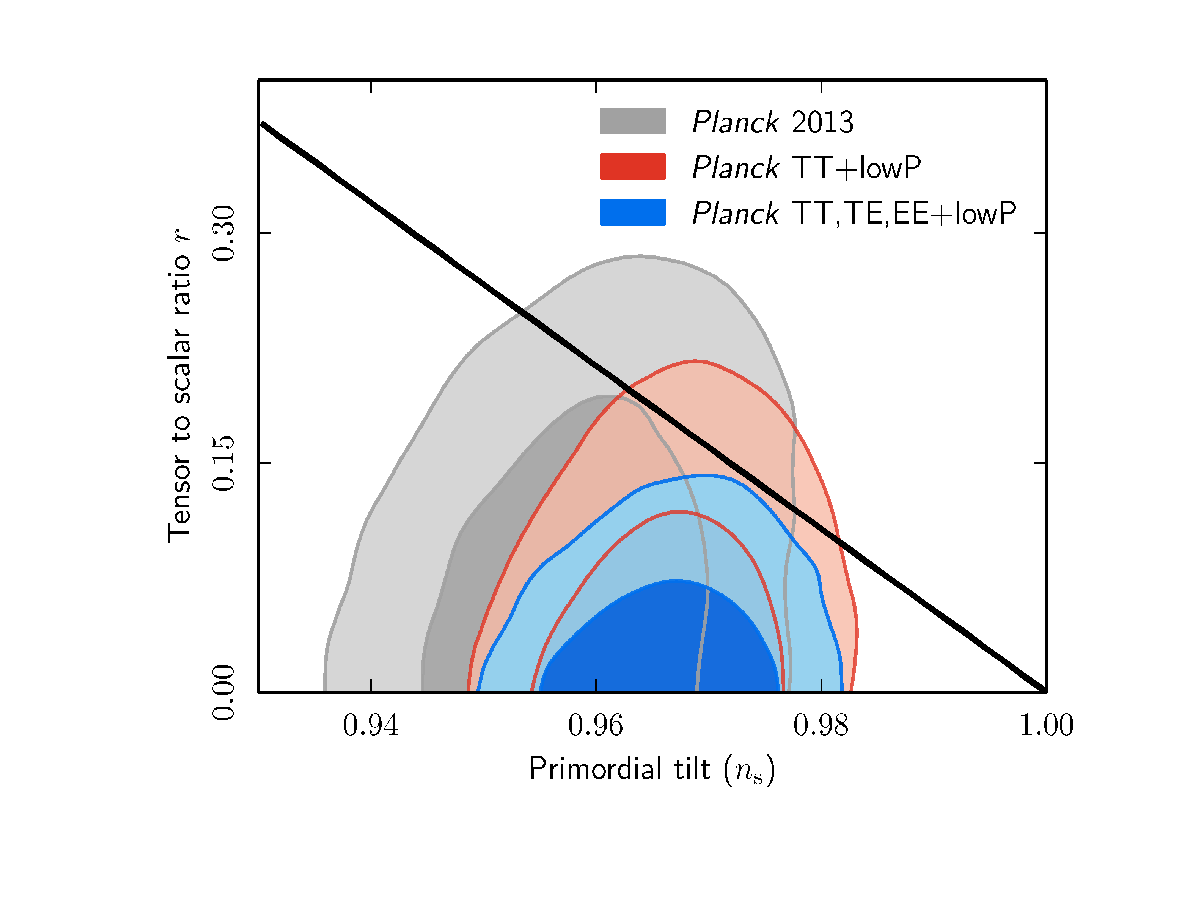
Figure 1: Marginalized joint confidence contours for $(n_{\mathrm{s}}\,,r)$, at the 68 % and 95 % CL, in the presence of running of the spectral indices. The black path corresponds to the curve $(n_{s}(x),r(x)))$ of our model (Figure courtesy of the Planck2015 Collaboration).

To determine the value of the parameter $\bar{\lambda}$, one has to take into account the theoretical btw and the observational bld values of the power spectrum when the pivot scale, namely $k_{*}$, crosses the Hubble radius

$${\mathcal{P}}\cong\frac{H^{2}_{*}}{8\pi^{2}M_{pl}^{2}\epsilon}\cong\frac{24\bar{\lambda}^{4}}{\pi^{2}x^{3}}\cong 2\times 10^{-9},$$ (25)

where $H_{*}$ denotes the value of the Hubble parameter when the pivot scale leaves the Hubble radius. Finally, using the values of $x$ in the range $[0.0075,0.0156]$, we conclude that

$$\bar{\lambda}\sim 10^{-4}.$$ (26)

To get more in touch with observational data, we note that, for a given $k$-mode, we can write

$$\frac{k}{a_{0}H_{0}}=e^{-N_{k}}\frac{H_{k}}{H_{0}}\frac{a_{end}}{a(0)}\frac{a(0)}{a_{R}}\frac{a_{R}}{a_{M}}\frac{a_{M}}{a_{0}}=e^{-N_{k}}\frac{H_{k}}{H_{0}}\frac{a_{end}}{a(0)}\frac{\rho_{R}^{-1/12}\rho_{M}^{1/4}}{\rho^{1/6}(0)}\frac{a_{M}}{a_{0}},$$ (27)

where $R$ (resp. $M$) denotes the point when radiation (resp. matter) starts to dominate, $N_{k}$ is the number of e-folds from the $k$-mode exiting the Hubble radius to the end of inflation, $H_{k}$ is the value of the Hubble parameter when the $k$-mode leaves the Hubble radius, and we have used the relation between the scale factor and the energy density in the corresponding different phases

$$\left(\frac{a(0)}{a_{R}}\right)^{6}=\frac{\rho_{R}}{\rho(0)},\quad\left(\frac{a_{R}}{a_{M}}\right)^{4}=\frac{\rho_{M}}{\rho_{R}}.$$ (28)

Then, for modes in the current horizon scale $k=a_{0}H_{0}$, one has

$$N_{hor}=\ln\left(\frac{H_{hor}}{H_{0}}\right)+\ln\left(\frac{a_{end}}{a(0)}\right)+\frac{1}{4}\ln\left(\frac{\rho_{M}}{\rho_{R}}\right)+\frac{1}{6}\ln\left(\frac{\rho_{R}}{\rho(0)}\right)+\ln\left(\frac{a_{M}}{a_{0}}\right).$$ (29)

If we assume, as usual, that inflation ends when the universe starts to decelerate ($\epsilon=1)$, this means $\dot{H}=-H^{2}$; in our model, this will happen when $e^{-8\sqrt{3}M_{pl}\bar{\lambda}^{2}t_{end}}\cong 10$, thus, $H_{end}\cong\frac{20M_{pl}\bar{\lambda}^{2}}{\sqrt{3}}$ and $a_{end}=0.35a(0)$, and, therefore, $\ln\left(\frac{a_{end}}{a(0)}\right)\cong-1.04$.

Using $\frac{a_{0}}{a_{M}}=3360$ rg , one obtains $\ln\left(\frac{a_{M}}{a_{0}}\right)\cong-8.12$. Further, from (25) we also have

$$\ln\left(\frac{H_{hor}}{H_{0}}\right)\cong 130.75+\frac{1}{2}\ln x.$$ (30)

Now, since the current temperature of the cosmic background is $T_{0}=2.73$ K and the conservation of entropy implies $T_{M}=\frac{a_{0}}{a_{M}}T_{0}\sim 9\times 10^{3}$ K $\sim 9\times 10^{-10}$ GeV, using that $\left(\frac{\rho_{M}}{\rho_{R}}\right)^{1/4}\cong\frac{T_{M}}{T_{R}}$, we obtain that

$$\frac{1}{4}\ln\left(\frac{\rho_{M}}{\rho_{R}}\right)\cong-20.83-\ln\left(\frac{T_{R}}{\mbox{GeV}}\right).$$ (31)

Moreover, for our model it turns out that $\rho^{\frac{1}{4}}(0)\cong 2\bar{\lambda}M_{pl}\sim 2\times 10^{14}$ GeV. Then,

$$\frac{1}{6}\ln\left(\frac{\rho_{R}}{\rho(0)}\right)=\frac{2}{3}\left(-32.57+\ln\left(\frac{T_{R}}{\mbox{GeV}}\right)\right).$$ (32)

Finally, collecting all the results above, it follows that we obtain

$$N_{hor}\cong 79.04+\frac{1}{2}\ln x-\frac{1}{3}\ln\left(\frac{T_{R}}{\mbox{GeV}}\right),$$ (33)

what means that if the reheating temperature –with the purpose to ensure the success of nucleosynthesis– needs to belong in the range between $10^{9}$ GeV and $1$ MeV, then the number of e-folds must lie between $70$ and $80$. In particular, when the reheating temperature is of the order of $10$ MeV –the scale we obtain if reheating is due to the creation of heavy particles with masses of about $10^{12}$ GeV during the phase transition– the number of e-folds of the universe expansion in our model, from modes in the current horizon scale exiting the Hubble radius towards the end of inflation, is approximately $78$.

We observe that this number of e-folds is larger than the one obtained if it is assumed that there is not a substantial drop of energy density during the last stages of inflation ($\rho_{hor}\cong\rho_{end}$) and that the universe reheats immediately after the end of it ($\rho_{R}\cong\rho_{end}$). Then, a simple calculation leads to $N_{hor}\cong 68.25+\frac{1}{4}\ln\left(\frac{\rho_{hor}}{M_{pl}^{4}}\right)\cong 64.6+\frac{1}{4}\ln x\cong 62$ ll . In fact, from those results we can see that such assumptions are unjustified, because in our model the drop of energy density plus a reheating temperature compatible with nucleosynthesis leads to an increase of between $8$ and $12$ e-folds. Moreover, there is a key difference between standard inflation, where the potential has a minimum and particle production is due to the oscillations of the inflaton, and quintessential inflation, because in the first case it is usually assumed that from the end of inflation onto reheating the universe is matter dominated, leading to the formula ll

$$N_{hor}\cong 64.6+\frac{1}{4}\ln\epsilon+\frac{1}{4}\ln\left(\frac{\rho_{hor}}{\rho_{end}}\right)+\frac{1}{12}\ln\left(\frac{\rho_{R}}{\rho_{end}}\right),$$ (34)

which gives, for admissible reheating temperatures, between $50$ and $60$ e-folds. However, in quintessential inflation after the phase transition to reheating the universe is stiff matter dominated, leading to the expression (recall that in our model $x\cong\epsilon$)

$$N_{hor}\cong 64.6+\frac{1}{4}\ln\epsilon+\ln\left(\frac{a_{end}}{a(0)}\right)+\frac{1}{4}\ln\left(\frac{\rho_{hor}}{\rho(0)}\right)-\frac{1}{12}\ln\left(\frac{\rho_{R}}{\rho(0)}\right),$$ (35)

which, we have showed, gives between $70$ and $80$ e-folds. The main difference lies in the sign of the last term: in the first expression is positive, which means that the number of e-folds decreases, while in the second one it is negative, and thus, the number of e-folds will grow.

A final remarks are in order: Here we have calculated the number of e-folds for modes in the current horizon scale $k=a_{0}H_{0}$. However, if one chooses modes, as in the Ade , in the scale of $k=0.005$ $\mbox{Mpc}^{-1}$, then the number of e-folds is reduced in $5$ units, and thus, for our model, it will lie between $65$ and $75$. This result agrees with Planck2013 data (see figure 1), because as we have already explained, at $95.5\%$ C.L., for our model, Planck2013 data constrains the number of e-folds to lie between $64$ and $133$.

IV The reheating process

When dealing with the so-called inflationary non-oscillatory models fkl , i.e, models where the potential does not have an absolute minimum, preheating occurs due to a sudden phase transition from an inflationary phase to another one. There, the breakdown of adiabaticity leads to the production of particles coupled to gravity. For instance, in ford the production of massless nearly conformally coupled particles originated in a sudden transition from inflation to the radiation era is studied.

Here, we will discuss the production of heavy massive $\chi$-particles ($m\gg\bar{\lambda}^{2}M_{pl}$) conformally coupled to gravity coming from a phase transition to a kination regime (see he for details).

Working in Fourier space, the dynamical equation of the $\chi$-particles is the same as an harmonic oscillatory

$$\chi_{k}^{\prime\prime}+\omega^{2}_{k}(\tau)\chi_{k}=0,$$ (36)

where the derivatives are taken with respect to the conformal time $\tau$ and the time dependent frequency of the $k$-mode is given by $\omega_{k}(\tau)=\sqrt{k^{2}+m^{2}a^{2}(\tau)}$.

In this case, since for our model (12) the second derivative of the Hubble parameter is nearly continuous at the transition point (the difference between the second derivative immediately before and after the phase transition being of order $\lambda^{2}\bar{\lambda}^{4}M_{pl}^{3}\sim 10^{-77}M_{pl}^{3}$), to take into account particle production during the adiabatic regimes, one has to use the second-order WBK solution (the first order WKB solution only contains first order derivatives of the Hubble parameter that, for our models, are always continuous, meaning that using this approximation it is impossible to take into account particle production) with the purpose to approximately define, before the transition time, the vacuum modes Haro

$$\chi_{2,k}^{WKB}(\tau)\equiv\frac{1}{\sqrt{2W_{2,k}(\tau)}}e^{-{i}\int^{\tau}W_{2,k}(\bar{\tau})d\bar{\tau}},$$ (37)

where the analytic expression of $W_{2,k}$ was calculated in Bunch

$$W_{2,k}=\omega_{k}-\frac{m^{2}a^{4}}{4\omega_{k}^{3}}(\dot{H}+3H^{2})+\frac{5m^{4}a^{6}}{8\omega_{k}^{5}}H^{2}+\frac{m^{2}a^{6}}{16\omega_{k}^{5}}(\dddot{H}+15\ddot{H}H+10\dot{H}^{2}+86\dot{H}H^{2}+60H^{4})$$

$$-\frac{m^{4}a^{8}}{32\omega_{k}^{7}}(28\ddot{H}H+19\dot{H}^{2}+394\dot{H}H^{2}+507H^{4})+\frac{221m^{6}a^{10}}{32\omega_{k}^{9}}(\dot{H}+3H^{2})H^{2}-\frac{1105m^{8}a^{12}}{128\omega_{k}^{11}}H^{4}.$$ (38)

Note that, near the transition time, the adiabatic condition $\frac{\omega_{k}^{\prime}}{\omega^{2}_{k}}\ll 1$ (the derivative is taken with respect to the conformal time) is fulfilled, because one has

$$\frac{\omega_{k}^{\prime}}{\omega^{2}_{k}}=\frac{m^{2}a^{3}H}{\omega^{3}_{k}}\sim\frac{H}{m}\sim\frac{\bar{\lambda}^{2}M_{pl}}{m}\ll 1,$$ (39)

what justifies the use of (37) to approximate the vacuum modes near the transition time. However, at the transition time the positive and negative frequencies mix, and after the abrupt phase transition the vacuum modes become approximately

$$\alpha_{k}\chi_{2,k}^{WKB}(\tau)+\beta_{k}(\chi_{2,k}^{WKB})^{*}(\tau),$$ (40)

where $\alpha_{k}$ and $\beta_{k}$ are Bogoliubov coefficients.

Then, impossing the continuity of the first derivative of (37) and (40) at the transition time, one obtains the system

$$\left\{\begin{array}[]{ccc}\chi_{2,k}^{WKB}(\tau_{E}^{-})&=&\alpha_{k}\chi_{2,k}^{WKB}(\tau_{E}^{+})+\beta_{k}(\chi_{2,k}^{WKB})^{*}(\tau_{E}^{+})\\ \frac{d}{d\tau}\chi_{2,k}^{WKB}(\tau_{E}^{-})&=&\alpha_{k}\frac{d}{d\tau}\chi_{2,k}^{WKB}(\tau_{E}^{+})+\beta_{k}\frac{d}{d\tau}(\chi_{2,k}^{WKB})^{*}(\tau_{E}^{+}),\end{array}\right.$$ (43)

where $\chi_{2,k}^{WKB}(\tau_{E}^{-})$ (resp. $\chi_{2,k}^{WKB}(\tau_{E}^{+})$) is the value of $\chi_{2,k}^{WKB}(\tau)$ before (resp. after) the phase transtion time $\tau_{E}$. Simple algebra shows that the $\beta_{k}$-Bogoliubov coefficient is given by (see Haro ; he )

$$\beta_{k}=\frac{{\mathcal{W}}[\chi_{2,k}^{WKB}(\tau_{E}^{-}),\chi_{2,k}^{WKB}(\tau_{E}^{+})]}{{\mathcal{W}}[(\chi_{2,k}^{WKB})^{*}(\tau_{E}^{+}),\chi_{2,k}^{WKB}(\tau_{E}^{+})]},$$ (44)

where ${\mathcal{W}}[f(\tau_{E}^{-}),g(\tau_{E}^{+})]\equiv f(\tau_{E}^{-})g^{\prime}(\tau_{E}^{+})-f^{\prime}(\tau_{E}^{-})g(\tau_{E}^{+})$ is the Wronskian of the functions $f$ and $g$ at time $\tau_{E}$.

Taking into account that the only discontinuous term in (IV) is $\frac{m^{2}a^{6}\dddot{H}}{16\omega_{k}^{5}}$, it is not difficult to show that the squared modulus of the Bogoliubov coefficient is given by

$$|\beta_{k}|^{2}\cong\frac{m^{4}a_{E}^{12}\left(\dddot{H}(0^{+})-\dddot{H}(0^{-})\right)^{2}}{1024(k^{2}+m^{2}a^{2}(0))^{6}},$$ (45)

where $\dddot{H}(0^{-})$ (resp. $\dddot{H}(0^{+})$), is the value of the second derivative of the Hubble parameter before (after) the phase transition. Recall that, for our model, this quantity is discontinuous at the transition time.

From here, using that $\int_{0}^{\infty}\frac{y^{2}}{(y^{2}+1)^{6}}dy=\frac{7!!}{10!!}\frac{\pi}{2}$, the number density of produced particles and their energy density are, respectively, Birrell

$$n_{\chi}(t)\equiv\frac{1}{2\pi^{2}a^{3}(t)}\int_{0}^{\infty}k^{2}|\beta_{k}|^{2}dk\sim 5\bar{\lambda}^{6}M_{pl}^{3}\left(\frac{\bar{\lambda}^{2}M_{pl}}{m}\right)^{5}\left(\frac{a(0)}{a(t)}\right)^{3},\rho_{\chi}(t)\equiv\frac{1}{2\pi^{2}a^{4}(t)}\int_{0}^{\infty}\omega_{k}(t)k^{2}|\beta_{k}|^{2}dk\sim mn_{\chi}(t).$$ (46)

Since these heavy particles are far from thermal equilibrium, they will decay into lighter particles, which will interact through multiple scattering, and thus, redistribute their energies to achieve a relativistic plasma phase in thermal equilibrium (for a more detailed explanation, see 37 ; 38 ).

To calculate the moment when thermalization occurs, we will use the thermalization process depicted in 38 , where the cross section is given by $\sigma={\alpha^{3}}\rho_{\chi}^{-\frac{1}{2}}(0)$, with $\alpha^{2}\sim 10^{-3}$. Then, the thermalization rate is

$$\Gamma=\sigma n_{\chi}(0)=\alpha^{3}\left(\frac{n_{\chi}(0)}{m}\right)^{\frac{1}{2}}\sim\alpha^{3}\left(\frac{\bar{\lambda}^{2}M_{pl}}{m}\right)^{3}\bar{\lambda}^{2}M_{pl}.$$ (47)

Equilibrium is reached when $\Gamma\sim H(t_{eq})=\bar{\lambda}^{2}M_{pl}\left(\frac{a(0)}{a_{eq}}\right)^{3}$, obtaining $\frac{a(0)}{a_{eq}}\sim\alpha\frac{\bar{\lambda}^{2}M_{pl}}{m}$. Thus, at the time of equilibrium, the energy densities of the produced particles and background are, respectively,

$$\rho_{\chi}(t_{eq})\sim 5\alpha^{3}\bar{\lambda}^{8}\left(\frac{\bar{\lambda}^{2}M_{pl}}{m}\ \right)^{7}{M_{pl}^{4}},\quad\rho(t_{eq})\sim 3\alpha^{6}\bar{\lambda}^{4}\left(\frac{\bar{\lambda}^{2}M_{pl}}{m}\ \right)^{6}M_{pl}^{4}.$$ (48)

After this thermalization, the relativistic plasma evolves as $\rho_{\chi}(t)=\rho_{\chi}(t_{eq})\left(\frac{a_{eq}}{a(t)}\right)^{4}$, and the background evolves as $\rho(t)=\rho(t_{eq})\left(\frac{a_{eq}}{a(t)}\right)^{6}$, because we are in the kination regime. Reheating is obtained when both energy densities are of the same order, and this will happen when $\frac{a_{eq}}{a_{R}}\sim\sqrt{\frac{\rho_{\chi}(t_{eq})}{\rho(t_{eq})}}$. Thus, we obtain a reheating temperature of the order

$$T_{R}\sim\rho_{\chi}^{\frac{1}{4}}(t_{eq})\sqrt{\frac{\rho_{\chi}(t_{eq})}{\rho(t_{eq})}}\sim\alpha^{-\frac{3}{4}}\bar{\lambda}^{4}\left(\frac{\bar{\lambda}^{2}M_{pl}}{m}\ \right)^{\frac{9}{4}}M_{pl}\sim 10^{3}\left(\frac{\bar{\lambda}^{2}M_{pl}}{m}\ \right)^{\frac{9}{4}}\mbox{ GeV}.$$ (49)

As an example, if we consider heavy particles with mass $m\sim 10^{12}$ GeV (recall that the condition $m\gg\bar{\lambda}^{2}M_{pl}$, implies $m\gg 10^{10}$ GeV), the temperature reduces to $T_{R}\sim 3\times 10$ MeV, that is, we obtain a temperature in the MeV regime.

Note that there are different thermalization processes. For example, in 37 the authors propose the following thermalization rate $\Gamma=\alpha^{2}n_{\chi}^{\frac{1}{3}}$, which has been used recently in hap in order to calculate the reheating temperature. In fact, for that process the reheating temperature is approximately

$$T_{R}\sim\sim 10^{4}\left(\frac{\bar{\lambda}^{2}M_{pl}}{m}\ \right)^{\frac{19}{8}}\mbox{ GeV},$$ (50)

which for masses satisfying $m\sim 10^{12}$ GeV, is of the order of $10^{2}$ MeV.

Finally, since we have the explicit form of the Hubble parameter in (12), we can calculate the time when reheating occurs, via the equality

$$3M_{pl}^{2}H^{2}(t_{R})\sim\alpha^{-3}\bar{\lambda}^{16}\left(\frac{\bar{\lambda}^{2}M_{pl}}{m}\ \right)^{{9}}M_{pl}^{4}.$$ (51)

Using the approximation $e^{-4\sqrt{3}\lambda^{2}M_{pl}t_{R}}\cong 1-4\sqrt{3}\lambda^{2}M_{pl}t_{R}$, one can see that $H(t_{R})\sim t_{R}^{-1}$, and thus

$$t_{R}\sim\alpha^{\frac{3}{2}}\bar{\lambda}^{-8}\left(\frac{\bar{\lambda}^{2}M_{pl}}{m}\ \right)^{-\frac{9}{2}}\frac{1}{M_{pl}}.$$ (52)

In the case of particles with mass $m\sim 10^{12}$ GeV, using that $t_{pl}\sim 5\times 10^{-44}s$, we obtain that the time from the phase transition to the end of reheating is of the order of

$$t_{R}\sim 5\times 10^{38}\frac{1}{M_{pl}}\sim 2\times 10^{-5}s.$$ (53)

In the same way we can calculate when the equilibrium will occur, via the identity $\rho(t_{eq})=3H^{2}(t_{eq})M_{pl}^{2}$, thus obtaining

$$H(t_{eq})\sim\alpha^{3}\bar{\lambda}^{2}\left(\frac{\bar{\lambda}^{2}M_{pl}}{m}\ \right)^{3}{M_{pl}}\Longrightarrow t_{eq}\sim\alpha^{-3}\bar{\lambda}^{-2}\left(\frac{\bar{\lambda}^{2}M_{pl}}{m}\ \right)^{-3}\frac{1}{M_{pl}},$$ (54)

which, in the case $m\sim 10^{12}$ Gev, becomes $t_{eq}\sim 10^{-24}s$.

A last important remark is in order. In pv the authors proposed the following model

$$V(\varphi)=\left\{\begin{array}[]{ccc}\lambda_{1}(\varphi^{4}+M^{4})&\mbox{for}&\varphi\leq 0\\ \frac{\lambda_{1}M^{8}}{\varphi^{4}+M^{4}}&\mbox{for}&\varphi\geq 0,\end{array}\right.$$ (57)

where, to match with observations, the dimensionless constant $\lambda_{1}$ has to be of order $10^{-14}$.

Since the derivatives of the potential are continuous up to order three included, it turns out that the first discontinuity in the Hubble parameter appears in the fifth derivative. In fact, $\frac{d^{5}H(t_{E}^{+})}{dt^{5}}-\frac{d^{5}H(t_{E}^{-})}{dt^{5}}\sim\frac{\lambda_{1}\dot{\varphi}^{4}(t_{E})}{M_{pl}^{2}}$, where $t_{E}$ is the transition time.

In order to calculate this quantity, we need do some considerations. First of all, for our model 1 the Hubble parameter at the transition time is $H_{E}\cong\frac{4\bar{\lambda}^{2}M_{pl}}{\sqrt{3}}$, and since its value when the pivot scale leaves the Hubble radius is $H_{*}\cong\frac{8\sqrt{3}\bar{\lambda}^{2}M_{pl}}{\epsilon}$, the energy drops by approximately $\frac{H_{E}}{H_{*}}\cong\frac{\epsilon}{6}$. Second, we will assume that for the Peebles-Vilenkin model one has an energy drop of the same order. Then, being so that when the pivot scale leaves the Hubble radius all the energy density is potential one, we will have $H_{*}=\sqrt{\frac{V(\varphi)}{3}}\cong\frac{8\sqrt{\lambda_{1}}}{\sqrt{3}\epsilon}M_{pl}$, where we did approximate the potential by $V(\varphi)=\lambda_{1}\varphi^{4}$, and we have used the first equation of (22). We thus obtain that at the transition time the Hubble parameter is approximately $H_{E}\sim\frac{4\sqrt{\lambda_{1}}}{3\sqrt{3}}M_{pl}$, for such model. Finally, since at the transition time all the energy density is kinetic, we will have $\dot{\varphi}(t_{E})=\sqrt{6}H_{E}M_{pl}\sim\sqrt{\lambda_{1}}M^{2}_{pl}$, what means that $\frac{d^{5}H(t_{E}^{+})}{dt^{5}}-\frac{d^{5}H(t_{E}^{-})}{dt^{5}}\sim\lambda_{1}^{3}M_{pl}^{6}$.

On the other hand, using the WKB approximation at a higher order, it follows that the square modulus of the $\beta$-Bogoliubov coefficient is

$$|\beta_{k}|^{2}\sim\frac{m^{4}a_{E}^{16}\lambda_{1}^{6}M_{pl}^{12}}{(k^{2}+m^{2}a^{2}_{E})^{8}},$$ (58)

what means that in the Peebles-Vilenkin model the number density of particles produced at the transition time, namely $n_{\chi}^{PV}(t_{E})$, is given by

$$n_{\chi}^{PV}(t_{E})\sim\lambda_{1}^{\frac{3}{2}}\left(\frac{\sqrt{\lambda_{1}}M_{pl}}{m}\right)^{9}M_{pl}^{3}.$$ (59)

Note the relation $\lambda_{1}=4\bar{\lambda}^{4}$; thus, to compare both models one has to choose $\sqrt{\lambda_{1}}\sim 10^{-8}$. In this situation, dealing with particles of mass $m\sim 10^{12}$ GeV, we find $n_{\chi}^{PV}(t_{E})\sim 10^{-42}M_{pl}^{3}$ which is $8$ orders smallers than the number density of particles obtained in our model, and thus, we conclude that the Peebles-Vilenkin model leads to an abnormally small reheating temperature. Actually, following the same steps as above one finds, for that model, a reheating temperature of the order $T_{R}^{PV}\sim\alpha^{-\frac{3}{4}}\lambda_{1}\left(\frac{\sqrt{\lambda_{1}}M_{pl}}{m}\right)^{\frac{19}{4}}M_{pl}\sim 10^{3}\left(\frac{\sqrt{\lambda_{1}}M_{pl}}{m}\right)^{\frac{19}{4}}$ GeV. This means that for particles with mass $m\sim 10^{12}$ GeV, the reheating temperature, in the Peebles-Vilenkin model would be of the order $T_{R}^{PV}\sim 3\times 10^{-7}$ GeV $\sim 3\times 10^{2}$ eV $\sim 3\times 10^{6}$ K, which is in fact a very low temperature.

For further comparison, even lower reheating temperatures appear, in the above sense, in the models of Spokoiny , where some very smooth potentials are chosen in order to describe universes with an early inflationary period and a late-time acceleration, leading indeed to very small reheating temperatures. In all that papers, however, it is never assumed that reheating is due to particle production of heavy particles conformally coupled to gravity, on the contrary, it is arguably produced there by light particles not conformally coupled with gravity (recall that massless conformally coupled particles are never at play), and previous results about reheating obtained in ford ; Damour ; Giovannini are used. The problem is that these results are model dependent and that, in all of them, an abrupt phase transition is crucially assumed –in order to get the necessary high amount of particle production– what invalidates their application to models with a smooth phase transition (see the discussion in hap ).

V Evolution after reheating

At the reheating time the kinetic energy of the field will be of the same order of the energy density of the universe $\dot{\varphi}^{2}(t_{R})\sim\rho(t_{R})$, because the potential energy is given by $V(\varphi)=4\lambda^{4}M_{pl}^{4}\sim 10^{-121}M_{pl}^{4}$, which is smaller than the energy density at reheating.

To find the evolution of the scalar field after reheating, note that when the relativistic plasma starts to dominate, the Hubble parameter is given by

$$H(t)=\frac{H_{R}}{1+2(t-t_{R})H_{R}},$$ (60)

where $H_{R}\sim\frac{\sqrt{\rho(t_{R})}}{M_{pl}}\sim\frac{\dot{\varphi}(t_{R})}{M_{pl}}$, what means that the scalar field satisfies the equation

$$\ddot{\varphi}+\frac{3H_{R}}{1+2(t-t_{R})H_{R}}\dot{\varphi}=0,$$ (61)

which solution is

$$\dot{\varphi}(t)=\frac{\dot{\varphi}(t_{R})}{\left(1+2(t-t_{R})H_{R}\right)^{\frac{3}{2}}}.$$ (62)

Since matter decays as $a^{-3}$ and radiation as $a^{-4}$, the universe enters into a matter domination regime at $t_{M}$, which can be calculated as follows. As we have seen in Sect. 3, due to the adiabatic regime after the phase transition, the temperature at the beginning of matter domination will be $T_{M}\cong 9\times 10^{3}$ K. Then, using that $\rho(t_{M})\sim H^{2}(t_{M})M_{pl}^{2}\sim\frac{M_{pl}^{2}}{t_{M}^{2}}\sim T_{M}^{4}$, one gets $t_{M}\sim\frac{M_{pl}}{T_{M}^{2}}\sim 10^{54}\frac{1}{M_{pl}}\sim 10^{10}$ s $\sim 3\times 10^{2}$ y.

As a consequence, for times after $t_{M}$, the field satisfies the equation

$$\ddot{\varphi}+\frac{6H_{M}}{2+3(t-t_{M})H_{M}}\dot{\varphi}=0,$$ (63)

where $H_{M}\cong\frac{H_{R}}{1+2(t_{M}-t_{R})H_{R}}$ is the value of the Hubble parameter at the beginning of the matter domination epoch. The solution of (63) is

$$\dot{\varphi}(t)=\frac{\dot{\varphi}(t_{M})}{\left(2+3(t-t_{M})H_{M}\right)^{{2}}},$$ (64)

where now $\dot{\varphi}(t_{M})\cong\frac{\dot{\varphi}(t_{R})}{\left(1+2(t_{M}-t_{R})H_{R}\right)^{\frac{3}{2}}}$.

At some given time $t_{\Lambda}$ the cosmological constant starts to dominate; this happens when

$$H^{2}(t_{\Lambda})M_{pl}^{2}\sim\lambda^{4}M_{pl}^{4}\Longrightarrow(t_{\Lambda}-t_{M})^{-1}\sim\lambda^{2}M_{pl},$$ (65)

that is, when $t_{\Lambda}\sim t_{M}+10^{20}s\sim t_{M}+3\times 10^{12}y.$ Further, when the cosmological constant dominates the fied equation will be

$$\ddot{\varphi}+\sqrt{12}\lambda^{2}M_{pl}\dot{\varphi}=0,$$ (66)

which solution is

$$\dot{\varphi}(t)=\dot{\varphi}(t_{\Lambda})e^{-\sqrt{12}\lambda^{2}M_{pl}(t-t_{\Lambda})},$$ (67)

where

$$\dot{\varphi}(t_{\Lambda})=\frac{\dot{\varphi}(t_{M})}{(2+(t_{\Lambda}-t_{M})H_{M})^{2}}\sim\frac{\dot{\varphi}(t_{M})\lambda^{4}M_{pl}^{2}}{H_{M}^{2}}=\frac{\dot{\varphi}(t_{R})\lambda^{4}M_{pl}^{2}}{H_{R}^{2}}(1+2(t_{M}-t_{R})H_{R})^{\frac{1}{2}}$$

$$\sim\frac{\lambda^{4}M_{pl}^{4}}{\rho_{\chi}^{\frac{1}{2}}(t_{R})}(1+2(t_{M}-t_{R})H_{R})^{\frac{1}{2}}\ll\frac{\lambda^{3}M_{pl}^{3}}{\rho_{\chi}^{\frac{1}{4}}(t_{R})},$$ (68)

where we have use that $t_{M}-t_{R}\ll t_{\Lambda}-t_{M}\sim\lambda^{-2}\frac{1}{M_{pl}}.$

From this result, we conclude that at the time $t_{\Lambda}$ the ratio of the kinetic to the potential energy is bounded

$$R\equiv\frac{\dot{\varphi}^{2}(t_{\Lambda})}{\lambda^{4}M_{pl}^{4}}\ll\frac{\lambda^{2}M_{pl}^{2}}{\rho_{\chi}^{\frac{1}{2}}(t_{R})}\sim\alpha^{\frac{3}{2}}\left(\frac{\lambda}{\bar{\lambda}^{4}}\right)^{2}\left(\frac{\bar{\lambda}^{2}M_{pl}}{m}\ \right)^{-\frac{9}{2}}\sim 2\times 10^{-31}\left(\frac{\bar{\lambda}^{2}M_{pl}}{m}\ \right)^{-\frac{9}{2}}.$$ (69)

We realize that for heavy particles with mass $m\sim 10^{12}$ GeV, this ratio satisfies $R\ll 2\times 10^{-22}\ll 1$, meaning that at present time the kinetic energy of the field is sub-dominant and it will be the potential one which will drive the universe evolution.

VI Conclusions

We have considered a model that unifies inflation with the current cosmic acceleration via a single scalar field whose potential is the combination of a double well inflationary potential and a cosmological constant. The model provides a background that is free from a big bang singularity, and which can be studied analytically, as we have here shown. It exhibits an early inflationary period where, for observable modes, the universe inflates for a number of $70$ to $80$ e-folds. This number seems large as compared with the usual range of e-fold values used to discard inflationary models. The reason behind is that, in standard inflation, where the potential as a minimum of energy and particle production is due to the oscillations of the inflaton, the universe evolves, from the end of inflation to reheating, as if it were matter dominated. However, in quintessential inflation, from the phase transition all the way to reheating, the universe evolves instead as if it were driven by an stiff fluid, and it is this difference that is responsible for an increase in the number of e-folds in favor of non-oscillatory models.

At the end of the inflationary period, the universe experiences a sudden phase transition to a kination phase, where heavy massive particles are created which reheat the universe some $10^{-5}$ seconds after they appear. At that point the universe enters into a radiation regime that finishes, as we have calculated, some $300$ years after the phase transition, the universe then becoming matter dominated. This domination lasts, as has been here shown, for about $3\times 10^{12}$ years after the beginning of the matter domination stage, until the cosmological constant starts to rule the universe evolution, what is still happening today.

Acknowledgments. We would like to thank professor Yifu Cai for his comments, in particular concerning the past-incompleteness of our model. This investigation has been supported in part by MINECO (Spain), projects MTM2014-52402-C3-1-P and FIS2013-44881, by I-LINK1019 from CSIC, and by the CPAN Consolider Ingenio Project.

References

• (1) A.G. Reiss et al, Astron. J. 116, 1009 (1998) [arXiv:9805201].
S. Perlmutter et al, Astrophys. J. 517, 565 (1999) [arXiv:9812133].
• (2) C.B. Netterfield et al, Astrophys. J. 571 604 (2002) [arXiv:0104460].
N.W. Halverson et al, Astrophys. J. 568, 38 (2002) [arXiv:0104489].
• (3) A. Guth, Phys.Rev. D23, 347 (1981).
A. Linde, Phys.Lett. B108, 389 (1982).
A. Albrecht and P.J. Steinhardt, Phys. Rev. Lett. 48, 1220 (1982).
• (4) S. Nojiri and S.D. Odintsov, Phys. Rev. D68, 123512 (2003) [arXiv:0307288].
• (5) B. Spokoiny, Phys. Lett. B315, 40 (1993) [arXiv:9306008].
• (6) P.J.E. Peebles and A. Vilenkin, Phys.Rev. D59, 063505 (1999) [arXiv:9810509].
• (7) E. Elizalde, S. Nojiri, S. D. Odintsov and D. Saez-Gomez, Eur.Phys.J. C70, 351 (2010) [arXiv:1006.3387].
• (8) Yi-Fu Cai, J. Liu and H. Li, Phys. Lett. B690, 213 (2010) [arXiv:1003.4526].
• (9) J. de Haro, J. Amorós and S. Pan, Phys. Rev. D93, 084818 (2016) [arXiv: 1601.08175].
• (10) M. Joyce, Phys. Rev. D55, 1875 (1997).
• (11) A. D. Linde and D. A. Linde, Phys.Rev. D50, 2456 (1994) [arXiv:9402115].
A. Vilenkin, Phys.Rev.Lett. 72, 3137 (1994) [arXiv:9402085].
• (12) G.F. Giudice, E.W. Kolb and A. Riotto, Phys. Rev. D64 023508 (2001), [arXiv:0005123].
S. Hannestad, Phys. Rev. D70, 043506 (2004) [arXiv:0403291].
• (13) M. Kawasaki, K. Kohri and N. Sugiyama, Phys. Rev. Lett. 82, 4168 (1999) [arXiv:9811437].
• (14) P.H. Frampton, K.J. Ludwick and R.J. Scherrer, Phys. Rev. D68, 103503 (2003) [arXiv:1106.4996].
• (15) I. Brevik, E. Elizalde, S. Nojiri, and S.D. Odintsov. Phys. Rev. D84, 103508 (2011) [arXiv:1107.4642].
• (16) A. Borde, A.H. Guth and A. Vilenkin, Phys. Rev. Lett. 90, 151301 (2003) [arXiv:0110012].
• (17) S. Pan, J. de Haro, A. Paliathanasis and R.J. Slagter, [arXiv:1601.03955].
• (18) D. Battefeld and P. Peter, Phys. Rep. bf 12, 004 (2014) [arXiv:1406.2790].
• (19) Y.F. Cai, T. Qiu, Y.S. Piao M. Li and X. Zhang, JHEP 0710, 071 (2007) [arXiv:0704.1090].
T. Qiu, J. Evslin, Y.F. Cai, M. Li and X. Zhang, JCAP 10, 036 (2011) [arXiv:1108.0593].
C. Lin, R.H. Brandenberger and L.L. Perreault, JCAP 04, 019 (2011) [arXiv:1007.2654].
• (20) E. Wilson-Ewing, JCAP 1303, 026 (2013) [arXiv:1211.6269].
E. Wilson-Ewing, JCAP 1308, 015 (2013) [arXiv:1306.6582].
Yi-Fu Cai, Jerome Quintin, Emmanuel N. Saridakis, Edward Wilson-Ewing, JCAP 1407, 033 (2014) [arXiv:1404.4364].
J. Haro and J. Amoros, JCAP 1412, 031 (2014) [arXiv:1406.0369].
• (21) B.A. Bassett, S. Tsujikawa and D. Wands, Rev.Mod.Phys. 78, 537 (2006) [arXiv:0507632].
• (22) P. A. R. Ade et al. [Planck Collaboration], Astron. Astrophys.  571, A22 (2014) [arXiv:1303.5082].
• (23) P. A. R. Ade et al. [Planck Collaboration], [arXiv:1502.02114] (2015).
• (24) E.F. Bunn, A.R. Liddle and M. J. White, Phys. Rev.D54, 5917 (1996).
• (25) T. Rehagen, G. B. Gelmini, (2015) [arXiv:1504.03768].
• (26) A.R Liddle and S.M. Leach, Phys.Rev. D68, 103503 (2003) [arXiv:0305263].
• (27) G. Felder, L. Kofman and A. Linde, Phys. Rev. D60, 103505 (1999) [arXiv:9903350]
• (28) L.H. Ford, Phys. Rev. D35, 2955 (1987).
• (29) J. Haro and E. Elizalde, JCAP 10, 028 (2015) [arXiv:1505.07948].
• (30) J. Haro, J. Phys. A: Mat. Theor. 44 205401 (2011).
• (31) T.S. Bunch, J. Phys A: Math. Gen. 13, 1297 (1980).
S. Habib, C. Molina-París and E. Motola, Phys. Rev. D61, 024010 (2002) [arXiv:9906120].
• (32) N.D. Birrell and C.P.W. Davies, Quantum Fields in Curved Space (Cambridge: Cambridge University Press) (1982).
• (33) R. Allahverdi and M. Drees, Phys. Rev. D66, 063513 (2002) [arXiv:0205246].
• (34) R. Allahverdi, R. Brandenberger, F.-Y. Cyr-Racine and A. Mazumdar, Ann. Rev. Nucl. Part. Sci. 60, 27 (2010) [arXiv:1001.2600].
• (35) T. Damour and A. Vilenkin, Phys.Rev.D53, 2981 (1995) [arXiv:9503149].
• (36) M. Giovannini, Phys.Rev.D58, 083504 (1998) [arXiv:9806329].