Radio disappearance of the magnetar XTE J1810$-$197 and continued X-ray timing

Abstract

We report on timing, flux density, and polarimetric observations of the transient magnetar and 5.54 s radio pulsar XTE J1810$-$197 using the Green Bank, Nançay, and Parkes radio telescopes beginning in early 2006, until its sudden disappearance as a radio source in late 2008. Repeated observations through 2016 have not detected radio pulsations again. The torque on the neutron star, as inferred from its rotation frequency derivative $\dot{\nu}$, decreased in an unsteady manner by a factor of 3 in the first year of radio monitoring, until approximately mid-2007. In contrast, during its final year as a detectable radio source, the torque decreased steadily by only 9%. The period-averaged flux density, after decreasing by a factor of 20 during the first 10 months of radio monitoring, remained relatively steady in the next 22 months, at an average of $0.7\pm 0.3$ mJy at 1.4 GHz, while still showing day-to-day fluctuations by factors of a few. There is evidence that during this last phase of radio activity the magnetar had a steep radio spectrum, in contrast to earlier flat-spectrum behavior. There was no secular decrease that presaged its radio demise. During this time the pulse profile continued to display large variations, and polarimetry, including of a new profile component, indicates that the magnetic geometry remained consistent with that of earlier times. We supplement these results with X-ray timing of the pulsar from its outburst in 2003 up to 2014. For the first 4 years, XTE J1810$-$197 experienced non-monotonic excursions in frequency derivative by at least a factor of 8. But since 2007, its $\dot{\nu}$ has remained relatively stable near its minimum observed value. The only apparent event in the X-ray record that is possibly contemporaneous with the radio shut-down is a decrease of $\approx 20\%$ in the hot-spot flux in 2008–2009, to a stable, minimum value. However, the permanence of the high-amplitude, thermal X-ray pulse, even after the (unexplained) radio demise, implies continuing magnetar activity.

1. Introduction

Magnetars are ultra-highly magnetized neutron stars (inferred surface dipolar field strengths $B_{s}\approx 10^{14-15}$ G) that display hugely variable and sometimes very bright X-ray emission, powered by their decaying fields (Duncan & Thompson, 1992). This process is reflected in their extremely unsteady rotation. Their magnetic fields cause magnetars to spin down very rapidly, and all those known have long periods, $2<P<12$ s.

Among the 23 known magnetars (Olausen & Kaspi, 2014), four are known to be transient emitters of radio pulsations. The first to be so identified was the $P=5.54$ s anomalous X-ray pulsar (AXP) XTE J1810$-$197, discovered in early 2003 following an X-ray outburst (Ibrahim et al., 2004). It is unclear when radio emission started, but pulsations were not present in 1998, while a point source was visible by early 2004 (Halpern et al., 2005). Radio pulsations were detected in early 2006 (Camilo et al., 2006), with some properties that are markedly different from those of ordinary rotation-powered pulsars, including extremely variable flux densities and pulse profiles, and flat spectra (e.g., Camilo et al., 2007d; Lazaridis et al., 2008). The emission is also highly linearly polarized, like that of several ordinary young radio pulsars (Camilo et al., 2007b; Kramer et al., 2007). To a great extent, these properties are shared by all four radio magnetars identified so far (Camilo et al., 2007a, 2008; Levin et al., 2010; Keith et al., 2011; Shannon & Johnston, 2013).

The radio emission from XTE J1810$-$197 arose following the X-ray outburst. The X-ray flux then decayed exponentially and returned to pre-outburst levels in 2007–2008 (Bernardini et al., 2011). Here we show that XTE J1810$-$197 ceased to emit detectable radio pulsations in late 2008, and present the timing, flux density, polarimetric, and pulse profile behavior during its last 20 months of radio activity. We also present X-ray timing measurements and fluxes through 2014.

2. Radio Observations

Our previously published radio studies of XTE J1810$-$197 (also known as PSR J1809$-$1943) are based on extensive data sets largely from 2006. Here we present results based on observations done with the Robert C. Byrd Green Bank Telescope (GBT), the Nançay radio telescope (NRT), and the CSIRO Parkes telescope, mainly through the end of 2008. Table 1 summarizes relevant parameters for all the radio observations presented in this paper.

Table 1Parameters and Sensitivities for Radio Observations of XTE J1810$-$197

	NRT	PKS AFB	PKS DFB	GBT
Center frequency (MHz)	1398	1374	1369	1950
Bandwidth (MHz)	64	288	256	600
Gain, $G$ (K Jy-1)	1.55	0.735	0.735	1.9
System temperature, $T_{\rm sys}$ (K)	47	44	44	28
SEFD (Jy)	30	60	60	15
$\eta$	1.0	$\sqrt{(\pi/2)}$	1.0	1.2
SEFDeff (Jy)	30	76	60	17

Note. — Observations used the Berkeley-Orléans-Nançay (BON) coherent dedispersor (Cognard & Theureau, 2006) at the NRT, the analog (AFB; Manchester et al., 2001) and digital (DFB; Manchester et al., 2013) filterbanks at Parkes, and the pulsar Spigot (Kaplan et al., 2005) at the GBT. Sensitivity parameters are given in the direction of XTE J1810$-$197 for the specified frequencies and bandwidths. The sky temperature at 1.4 GHz in this direction is $T_{\rm sky}=16.4$ K including CMB (obtained from http://www3.mpifr-bonn.mpg.de/survey.html; Reich et al. 2001).

2.1. Radio Timing

In Camilo et al. (2007c) we showed the timing behavior of XTE J1810$-$197 through 2007 January, based largely on 1.4 GHz data collected with the BON spectrometer at the NRT. As the flux density decreased it became preferable to time the pulsar at the GBT. We did this at 2 GHz using the Spigot spectrometer, recording the data in search mode and folding offline. Nevertheless, BON timing continued to be important, particularly during 2007 May–August when the GBT was not available. The NRT observations were coherently dedispersed, with the full band divided into 16 frequency channels, then folded at the predicted pulsar period with 2 minute sub-integrations before mid-2007 and 30 s thereafter. See Table 2 for a log of the timing observations newly presented here. Daily observations typically lasted 1 hr at Nançay and varied greatly at the GBT, from 0.25 hr to 2 hr with most at least 0.5 hr (i.e., from a couple of hundred to over 1000 pulsar rotations per session).

Table 2 Log of Radio Timing Observations of XTE J1810$-$197

MJD range (days)	Number of daily TOAs	Telescope
54128–54218 (90)	$53+18$	$\mbox{GBT}+\mbox{Nan\c{c}ay}$
54226–54357 (131)	27	Nançay
54352–54739 (387)	51	GBT

Note. — GBT TOAs were obtained with Spigot at 2 GHz; Nançay TOAs were obtained with BON at 1.4 GHz (see Section 2.1). The average observing cadence in the three periods listed decreased from once every 1.5 days, to once every 5 days, to once every 7.5 days.

In principle there are unusual challenges involved in radio timing of XTE J1810$-$197, because of changing pulse profiles. In practice we found that on the vast majority of days a simple procedure was sufficient to obtain times-of-arrival (TOAs) that could be used to describe reliably the rotation of the star. We first excised strong radio frequency interference from the BON and Spigot data. BON timing was detailed in Camilo et al. (2007c). For Spigot we obtained TOAs by cross-correlating individual folded pulse profiles with a Gaussian template. We then used the TOAs with the TEMPO software to obtain timing solutions.

Figure 1.— Torque and radio flux density of XTE J1810$-$197. (a) Frequency derivative versus date (Section 2.1). Measurements from before MJD 54127 (2007.1) are reproduced from Camilo et al. (2007c). (b) Period-averaged flux density versus date. Data from before 2007.1 were presented in Camilo et al. (2007c) but have been reanalyzed for this paper (see Section 2.2).

The position of XTE J1810$-$197 was held fixed in all our timing fits at that determined from VLBI observations (Helfand et al., 2007); the measured proper motion is too small to affect the timing of this pulsar. As explained in Camilo et al. (2007c), we maintained phase connection for this pulsar since 2006 April, but the rotation frequency derivative was changing so rapidly that it proved more informative to measure $\dot{\nu}$ (where $\nu=1/P$) by using TOAs typically spanning one month and doing a TEMPO fit for only $\nu$ and $\dot{\nu}$. We did such fits in segments of data offset by roughly 15 days to provide good sampling of $\dot{\nu}$, and the results are shown in Figure 1a. In this panel, the first 17 measurements are reproduced from Camilo et al. (2007c), while the next 33 measurements are new.

Figure 2.— Timing residuals for XTE J1810$-$197. (a) Phase residuals versus date for a timing model that fits only for rotation phase, frequency, and frequency derivative, showing a cubic trend. (b) Residuals for a model that fits for phase, $\nu$, $\dot{\nu}$, and $\ddot{\nu}$ (see Section 2.1 and Table 3).

Table 3 Two Radio Timing Solutions for XTE J1810$-$197

Parameter	Value
R.A. (J2000.0)	$18^{\rm h}09^{\rm m}51\fs 087$
Decl. (J2000.0)	$-19\arcdeg 43\arcmin 51\farcs 93$
Dispersion measure, DM	178.0 pc cm-3
Epoch (MJD TDB)	54550.0
Range of dates (MJD)	54352–54729
Frequency, $\nu$	0.18048830377(8) Hz
Frequency derivative, $\dot{\nu}$	$-9.163(1)\times 10^{-14}$ Hz s-1
Frequency, $\nu$	0.1804882977(1) Hz
Frequency derivative, $\dot{\nu}$	$-9.090(2)\times 10^{-14}$ Hz s-1
Frequency second derivative, $\ddot{\nu}$	$2.46(5)\times 10^{-22}$ Hz s-2
RMS post-fit timing residual ($P$)	0.007

Note. — The celestial coordinates were held fixed at the values obtained from VLBA observations (Helfand et al., 2007), and the DM was held fixed at the value obtained from simultaneous 0.7 and 2.9 GHz observations (Camilo et al., 2006).

It is clear from Figure 1a that over the last $\sim 400$ days $\dot{\nu}$ stabilized greatly, compared to earlier large variations. To investigate this in detail we obtained phase-connected fits spanning the last year of timing data. In Figure 2a we show the residuals from a simple fit to rotation phase, $\nu$, and $\dot{\nu}$, showing large residuals. In Figure 2b, we see that the addition of $\ddot{\nu}$ absorbs all remaining residual trends. These timing solutions are listed in Table 3. The positive value of $\ddot{\nu}$ implies that during this span $-\dot{\nu}$ (proportional to the braking torque) was decreasing steadily, by a total of 9% during the year.

2.2. Radio Flux Densities

One unusual aspect of radio emission from XTE J1810$-$197 is the fluctuation on $\sim$ daily timescales of its period-averaged flux density, largely intrinsic to the pulsar (e.g., Lazaridis et al., 2008). These variations result from a combination of different pulse profile components becoming active (i.e., because of radically changing profiles) and varying intensity from particular components. Superimposed on this apparently chaotic variation, the average flux density of the pulsar decreased by over an order of magnitude in the 10 months following its pulsed radio discovery, as seen in Figure 1b (these pre-2007 data were originally presented in Camilo et al. 2007c but have been reanalyzed here in order to present a consistent flux density record).

Most period-averaged flux densities presented in this paper (including all in Figure 1b) were obtained by measuring for each daily observation the area under the pulse profile, scaled to its off-pulse rms, and converting to a Jansky scale using the observing parameters and telescope system noise (cf. the SEFD_eff values in Table 1; see section 7.3.2 of Lorimer & Kramer 2004 for more details on this method). We estimate that the absolute 1.4 GHz flux density scale is accurate to within 10%.

The greatest source of uncertainty arises from the impact of radio frequency interference (RFI) and system noise fluctuations on this long period and, from 2007, faint pulsar. Each pulse profile was carefully excised of RFI in both the frequency and time domains. Nevertheless, for approximately one-third of all the post-2006 NRT observations, the RFI was so bad or the flux density was so low (approaching the $\approx 0.1$ mJy detection threshold), that we did not extract a flux density measurement at all. In some of the remaining instances, as much as half of the data had to be discarded in order to obtain an integrated profile clean enough to measure flux density. Mindful of these caveats (most often some residual RFI is bound to remain, and individual measurements could be greatly affected), we estimate that the NRT flux density measurements in Figure 1b have a typical relative fractional uncertainty of $\approx 20$%, with a minimum of 0.1 mJy.

Two things immediately stand out from Figure 1b: daily flux density variations continued through the end of our data set, by factors of a few; and the average 1.4 GHz flux density stabilized early in 2007, at a level of $0.68\pm 0.27$ mJy for all post-2006 NRT detections presented here. Also, the panels of Figure 1 are curiously something of a mirror image to each other.

2.2.1 Radio Disappearance

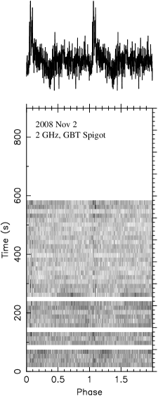
Figure 3.— Last radio detection of XTE J1810$-$197 at the GBT. The period-averaged flux density is among the smallest we observed ($\sim 50\,\mu$Jy), but pulse detection is aided by the “spiky” nature of its narrow sub-pulses. Two rotations are shown as a function of time, with the summed profile at the top. White areas are subintegrations masked due to particularly bad RFI.

Figure 4.— Fourty-seven radio non-detections of XTE J1810$-$197 since late 2008 (Section 2.2.1). The dots represent measured NRT flux densities, reproduced from Figure 1b. The other symbols denote individual observations without a detection, placed at approximately the upper flux density limits for the respective sets of observations.

With no warning from either its timing or flux density behavior, XTE J1810$-$197 ceased to emit detectable radio pulsations in late 2008. The last detection at the NRT was on October 29, on November 2 at the GBT (Figure 3), and at Parkes on the following day. The next attempt to detect it was on November 10. We attempted to detect the pulsar at Parkes on 20 occasions through 2016 January, largely at 1.4 GHz, each time for 0.5–1 hr. At the NRT we did 10 more observations through 2009 June. At the GBT we made a total of 17 attempts at 2 GHz, each $\approx 0.5$ hr, through 2012 August. The pulsar was not detected in any of these 47 observations spanning 7 years since 2008 November (Figure 4). We emphasize that XTE J1810$-$197 did not gradually fade into undetectability. A few weeks before the last detection, we recorded beautiful profiles (e.g., Figures 6d, 7c and 7d); the signal strength and pulse profiles were fluctuating at least as much as they had for the previous $\sim 500$ days. And then the radio pulses were gone.

For an assumed pulse duty cycle of 6% (comparable to the component widths often observed for this pulsar) and the parameters used in our monitoring observations (Table 1), the upper limit on the flux density of XTE J1810$-$197 since late 2008 is approximately 0.1 mJy at 1.4 GHz based on the NRT observations, slightly lower than that for the Parkes observations, and approximately 0.03 mJy at 2 GHz based on the GBT observations (Figure 4). These limits are nearly an order of magnitude below the average flux densities during the 1.8 years of radio emission post-2006, although not much below the faintest established detections (see Figures 3 and 5). The great profile variability, long period, and RFI, make more detailed estimates unreliable. In any case, since the last detection in late 2008, in none of 47 observations spanning 7 years was the pulsar as detectable as in the poorest of more than 200 detections made over a period of 2 years before 2008 November.

Figure 5.— Flux density measurements for XTE J1810$-$197 at 1.4 GHz and 2 GHz in 2007–2008. Parkes observations include those done with analog (AFB) and full-Stokes digital (DFB) filterbanks. See Section 2.3 for details.

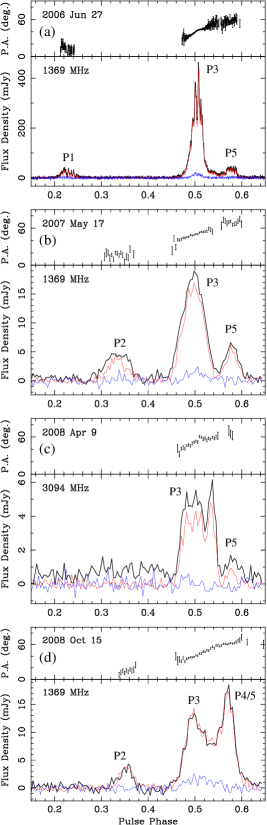
Figure 6.— Polarimetric pulse profiles of XTE J1810$-$197 recorded at Parkes. Only 50% of pulse phase is shown. In each lower panel the black trace represents total intensity, red is linear polarization, and blue is circular. Each upper panel shows the position angle of linear polarization, rotated to the pulsar frame using $\mbox{RM}=78$ rad m^-2. The profiles are phase-aligned with respect to each other by eye, and absolute phase is arbitrary. Recurring profile features are labelled P1–P5 (as in Figure 7).

2.3. Radio Spectrum

The available evidence suggests that during the faint epoch that lasted for 2 years preceding its radio disappearance in late 2008, XTE J1810$-$197 had a steep radio spectrum, contrasting to its earlier generally flat spectrum.

In Figure 5 we present all our post-2006 flux density measurements at 1.4 GHz and 2 GHz. The 1.4 GHz NRT values are reproduced from Figure 1b. These are fundamentally consistent with Parkes measurements at the same frequency from six full-Stokes observations using pulsar digital filterbanks (DFBs), analyzed with PSRCHIVE (Hotan et al., 2004), and 12 analog filterbank (AFB) observations.

The 2 GHz flux density values presented here were obtained from a subset of the GBT data used to derive TOAs (Section 2.1), using the method outlined in Section 2.2 for NRT and Parkes AFB observations. We determined the system noise (Table 1) from a full-Stokes 2 GHz observation in the direction of XTE J1810$-$197, flux-calibrated with PSRCHIVE. Even after careful RFI excision, we selected for reliable flux density measurements only 40% of all observations from which we extracted a TOA. We estimate relative fractional uncertainties of $\approx 20$% on average.

The 2 GHz measurements in Figure 5 range over 0.1–0.5 mJy, with an average and standard deviation of $S_{2}=0.25\pm 0.10$ mJy. This is to be compared to $S_{1.4}=0.68\pm 0.27$ mJy for the 1.4 GHz measurements in the figure (Section 2.2), spanning much the same time interval. At face value this would seem to suggest a spectral index of $\alpha\approx-3$ (where $S_{\nu}\propto\nu^{\alpha}$). Given the inherent difficulties in extracting such a measurement for this variable pulsar from non-simultaneous multi-frequency observations susceptible to RFI despite our best efforts, we do not claim a reliable numerical value for $\alpha$. But Figure 5 strongly suggests that XTE J1810$-$197 indeed became a steep-spectrum object during its final “weak” state prior to disappearance as a radio source, in that respect more akin to an ordinary pulsar than earlier in its “high” state, when the torque was also varying rapidly (Figure 1).

2.4. Polarimetry

All of our previously published XTE J1810$-$197 polarimetric data are from before 2006 December (Camilo et al., 2007b). The data published by Kramer et al. (2007) end even earlier, but include single-pulse polarimetry. Here we present some polarimetric observations done in 2007 and 2008 with Parkes at 1.4 GHz and 3 GHz, using respectively the center beam of the multibeam receiver and the 10 cm band of the 1050cm receiver. The data were collected using DFBs, and analyzed with PSRCHIVE, as in Camilo et al. (2007b).

Figure 6a is a reprocessed version of a 2006 observation presented in Camilo et al. (2007b), differing mainly in the flux density scale and amount of data excised due to RFI. The recalculated rotation measure is $\mbox{RM}=76\pm 1$ rad m^-2, entirely consistent with the value in Camilo et al. (2007b), and the RMs calculated for the latter observations are consistent with this value within their larger uncertainties.

The 3 GHz full-Stokes profile (Figure 6c) looks similar to its counterpart from 1.5 years before (Figure 1c of Camilo et al., 2007b). At 1.4 GHz, the two 2007/2008 profiles (Figure 6b and 6d) show very similar position angles of linear polarization (PA), and differ mainly in the relative amplitudes of three total-intensity profile components (labelled P2, P3, and P4/5). Both profiles are close to 100% linearly polarized.

Comparison between the 2006 profile (Figure 6a) and the 2007/2008 1.4 GHz profiles shows that the PA sweep and its absolute values are similar for the “main pulse” regions (components P3–P5). However, the 2007/2008 profiles show component P2 not present in the 2006 profile — whose P1 component in turn is not seen later on. Profile components P1–P5 altogether span 40% of pulse phase, and if they all display stable PAs between 2006 and 2007/2008, then in principle this allows for a more conclusive investigation of geometry than previously possible (see Section 4.1).

2.5. Radio Pulse Profiles

Figure 7.— A selection of XTE J1810$-$197 radio pulse profiles. Prominent features in the profile that reoccur are labelled P1–P5 (as in Figure 6). We define the “main pulse” (MP) region as being composed of up to features P3–P5. Profiles are aligned by eye, and the absolute phase here is arbitrary.

The total-intensity pulse profiles of XTE J1810$-$197 were always extremely variable, both in phase of active emitting regions and in the daily appearance of each pulse profile component. The description that follows is based on a review of hundreds of daily profiles that we obtained during 2006–2008 at the GBT, Parkes, and Nançay. There was never any stable pulse profile, but we detected emission from some pulse longitudes more often than from others, with some discernible patterns over time, and radio pulsations were never detected from many longitudes. In that sense, there was some long-lasting stability to the radio-emitting region.

Referring to Figure 7a, emission was always detected from the main pulse region (MP, in turn made up of at least three discernible sub-structures, labelled P3–P5, not all necessarily emitting at once). Emission from component P1 (see also Figure 6a) was detected only during 2006, and it was the most variable, sometimes being much brighter than the MP components. On the other hand, P2 was active sometimes in 2006 and 2007 (Figure 6b), but became more common in 2008 (Figures 6d and 7c–d). In 2007 the observed profile often consisted of emission from the MP region alone (Figure 7b). In only one (2006) observation out of hundreds did we detect emission from all these regions at once (Figure 7a).

The relative amplitudes of the different components varied widely, exemplified in Figure 7d by P4, usually not preeminent but on this day the brightest of any. The very “spiky” nature of the individual sub-pulses that built up the broader integrated profile components (see, e.g., Serylak et al., 2009) continued to the very end (Figure 3).

Our sense is that in 2007–2008 the profiles were less variable than in 2006, but this impression may be biased by two factors: the pulsar was much brighter in 2006, which allowed the detection of very faint rarely observed components (see Figure 2 of Camilo et al., 2007c); and the total integration (both in number and in average duration of observations) was larger in 2006 compared to later. In any case it is clear that during the period when the torque had stabilized by comparison to earlier huge variations, and when the period-averaged flux density had also stabilized in an average sense at a low level (Figure 1), the pulse profiles of XTE J1810$-$197 were still varying at unprecedented levels compared to normal pulsars, and continued to do so until radio pulsations disappeared.

3. X-ray Observations

In order to search for clues to the disappearance of radio pulsations from XTE J1810$-$197, we reviewed all its archival Chandra and XMM-Newton data collected from 2003–2014. Timing results from 2009 November onward are newly published here. Detailed spectroscopic and flux analysis are presented in Alford & Halpern (2016), with a summary of the fluxes given in Section 3.2. In summary, we find that the X-ray fluxes stepped down to a minimum value around the time that the radio pulsations shut off, and this is the only recognizable event in X-rays that is plausibly contemporaneous with the disappearance in radio.

3.1. X-ray Timing

Table 4Log of X-ray Timing Observations of XTE J1810$-$197

Mission/Instrument	ObsID	Date	Epoch	Exposure	Frequency
		(UT)	(MJD)	(ks)	(Hz)
Chandra HRC	4454	2003 Aug 27	52878	2.8	0.180531(11)
XMM-Newton pn+MOS	0161360301	2003 Sep 8	52890	12.1	0.18052682(30)
XMM-Newton pn	0152833201	2003 Oct 12	52924	8.9	0.1805245(12)
Chandra HRC	5240	2003 Nov 1	52944	2.8	0.180536(10)
XMM-Newton pn+MOS	0161360501	2004 Mar 11	53075	18.9	0.18052415(25)
XMM-Newton pn+MOS	0164560601	2004 Sep 18	53266	28.9	0.18051856(18)
XMM-Newton pn+MOS	0301270501	2005 Mar 18	53447	42.2	0.18051142(16)
XMM-Newton pn+MOS	0301270401	2005 Sep 20	53633	42.2	0.1805046(3)
XMM-Newton pn+MOS	0301270301	2006 Mar 12	53806	51.4	0.1804991(4)
Chandra ACIS-S	6660	2006 Sep 10	53988	30.1	0.1804942(14)
XMM-Newton pn+MOS	0406800601	2006 Sep 24	54002	50.3	0.18049355(34)
XMM-Newton pn+MOS	0406800701	2007 Mar 6	54165	68.3	0.18049117(27)
XMM-Newton pn+MOS	0504650201	2007 Sep 16	54359	74.9	0.18048987(19)
Chandra ACIS-S	7594	2008 Mar 18	54543	29.6	0.1804868(15)
XMM-Newton pn+MOS	0552800201	2009 Mar 5	54895	65.8	0.18048610(24)
XMM-Newton pn+MOS	0605990201	2009 Sep 5	55079	21.6	0.1804857(13)
XMM-Newton pn+MOS	0605990301	2009 Sep 7	55081	19.9	0.1804829(16)
XMM-Newton pn+MOS	0605990401	2009 Sep 23	55097	14.2	0.1804872(24)
Chandra ACIS-S	11102	2009 Nov 1	55136	25.1	0.1804852(16)
Chandra ACIS-S	12105	2010 Feb 15	55242	12.6	0.180476(6)
Chandra ACIS-S	11103	2010 Feb 17	55244	12.6	0.180484(6)
XMM-Newton pn+MOS	0605990501	2010 Apr 9	55295	9.9	0.1804820(48)
Chandra ACIS-S	12221	2010 Jun 07	55354	10.0	0.180489(8)
XMM-Newton pn+MOS	0605990601	2010 Sep 5	55444	11.3	0.1804771(40)
Chandra ACIS-S	13149	2010 Oct 25	55494	15.4	0.1804766(35)
Chandra ACIS-S	13217	2011 Feb 8	55600	15.0	0.1804835(35)
XMM-Newton pn+MOS	0671060101	2011 Apr 3	55654	22.9	0.1804796(13)
XMM-Newton pn+MOS	0671060201	2011 Sep 9	55813	15.9	0.1804751(18)
Chandra ACIS-S	13746	2012 Feb 19	55976	20.0	0.1804790(23)
Chandra ACIS-S	13747	2012 May 24	56071	20.0	0.1804774(21)
XMM-Newton pn+MOS	0691070301	2012 Sep 6	56176	17.9	0.1804721(17)
XMM-Newton pn+MOS	0691070401	2013 Mar 3	56354	17.9	0.1804722(18)
XMM-Newton pn+MOS	0720780201	2013 Sep 5	56540	24.5	0.1804721(12)
Chandra ACIS-S	15870	2014 Mar 1	56717	20.1	0.1804723(20)
XMM-Newton pn+MOS	0720780301	2014 Mar 4	56720	25.0	0.1804682(11)
Chandra ACIS-S	15871	2014 Sep 7	56911	20.1	0.1804710(23)

Figure 8.— X-ray timing and flux properties of XTE J1810$-$197 from Chandra and XMM-Newton. (a) Frequency measurements, where the points linked with the solid line in 2009–2012 comprise the phase-connected solution in Table 5. The dashed line segment is the radio timing solution from Table 3. (b) Frequency derivatives obtained by differencing adjacent frequency measurements, and from the 2009–2012 phase-connected solution. The vertical lines denote the first two epochs of radio detection at 1.4 GHz with the VLA (Halpern et al., 2005; Camilo et al., 2006), and the shaded region encompasses the epochs of pulsed radio detection from Figure 1. It is not known whether radio emission at the flux density level of the first detection ($4.5\pm 0.5$ mJy) was present earlier in the X-ray outburst, which was detected in 2003 January. (c) X-ray flux measurements from the three- or two-temperature blackbody fits of Alford & Halpern (2016). Open triangles are the sum of the varying hot and warm areas, and filled squares are the total flux including the triangles and the cooler full surface area of the neutron star represented by the (constant) dashed line.

Table 4 is a log of all XTE J1810$-$197 timing observations performed by Chandra and XMM-Newton through 2014. The Chandra ACIS observations were taken with the source on the S3 CCD, and with a subarray of 100 or 128 rows to obtain time resolution of 0.3 s or 0.4 s, respectively. XMM-Newton observations used the pn CCD in full-frame or large-window mode, with 74 ms or 44 ms resolution and, in most cases, the MOS CCDs in small-window mode with 0.3 s resolution. We corrected the processed archival XMM-Newton photons for leap seconds and time jumps when needed, and applied the barycentric correction at the VLBI measured position. We then computed frequencies and $1\,\sigma$ errors using the $Z_{1}^{2}$ test on photons in the 0.3–4 keV band. The two short Chandra HRC observations that were obtained for the purpose of source location have relatively uncertain frequencies, and were not used in the subsequent analysis.

The frequency measurements are shown in Figure 8a. These were used to track the time-varying frequency derivative from 2003–2009 by computing the difference in frequency between adjacent XMM-Newton observations, usually 6 months apart. Where these $\dot{\nu}$ measurements overlap with the more precise record obtained from radio observations during 2006–2008 (Figure 1a), they agree. Figure 8b illustrates that $\dot{\nu}$ varied by a factor of $\approx 6$. In the months immediately following the outburst, which was first detected in 2003 January, monitoring by RXTE showed noisy spin-down with an even higher mean frequency derivative of $-6.7\times 10^{-13}$ Hz s^-1 (Ibrahim et al., 2004), which is $\approx 8$ times the minimum value of $\approx-8\times 10^{-14}$ Hz s^-1 measured by XMM-Newton in 2007–2008 (Figure 8b).

Starting in 2009 September, more frequent observations allowed a phase-connected solution to be established up through 2012 May. This process was facilitated by the relatively stable spin-down with small rate at later times. Beginning with the two observations on 2009 September 5 and 7, we folded the photons jointly using the $Z_{1}^{2}$ test, and used the resulting frequency to fold the next observation, verifying that the predicted phase agrees with the observed one to $<0.2$ cycles. Each subsequent observation was then added to the joint fit and the $Z_{1}^{2}$ test was iterated with free parameters $\nu$ and $\dot{\nu}$, and finally $\ddot{\nu}$, until 15 observations were included. The resulting fit is shown by the solid line in Figure 8a, and its $\dot{\nu}=-9.21\times 10^{-14}$ Hz s^-1 (Table 5) is very nearly a continuation of the minimum spindown rate that was first reached in 2007. The second frequency derivative as listed in Table 5 is necessary to fit the 2009–2012 series with a continuous ephemeris.

Table 5X-ray Timing Solution for XTE J1810$-$197

Parameter	Value
R.A. (J2000.0)	$18^{\rm h}09^{\rm m}51\fs 087$
Decl. (J2000.0)	$-19\arcdeg 43\arcmin 51\farcs 93$
Epoch (MJD TDB)	55444.0
Range of dates (MJD)	55079–56071
Frequency, $\nu$	0.18048121539(63) Hz
Frequency derivative, $\dot{\nu}$	$-9.2121(35)\times 10^{-14}$ Hz s-1
Frequency second derivative, $\ddot{\nu}$	$4.1(3)\times 10^{-23}$ Hz s-2
Surface dipole magnetic field, $B_{s}$	$1.3\times 10^{14}$ G
Spin-down luminosity, $\dot{E}$	$6.6\times 10^{32}$ erg s-1
Characteristic age, $\tau_{c}$	31 kyr

Analyzing the same data from which we established the phase-connected ephemeris of Table 5, Pintore et al. (2016) claimed to identify a timing anomaly in which the pulsar was spinning up (positive $\dot{\nu}$) between 2010 September and 2011 February. This could have arisen from their underestimation of uncertainties in frequency measurements. In any case, our phase-coherent ephemeris spanning this time shows no such event. Pintore et al. (2016) also propose that there is a single phase-connected timing solution spanning all of 2007–2014. This is clearly invalid, because their listed uncertainties on the polynomial coefficients ($\nu$, $\dot{\nu}$, $\ddot{\nu}$) are two orders of magnitude larger than what would be needed to describe a unique cycle count. Also, the parameters of our actual phase-coherent timing segments in radio (Table 3) and X-ray (Table 5) disagree with theirs. In particular, their fitted $\dot{\nu}=-4.9\times 10^{-14}$ Hz s^-1 is about half of the true value.

After 2012 May we were unable to maintain phase connection. The prior coherent timing solution fails to predict the phase of the 2012 September observation by $\approx 0.5$ cycles. Possibly an anti-glitch (Archibald et al., 2013; Şaşmaz Muş et al., 2014) and/or change in torque occurred between 2012 May and September. But we cannot tell for sure what happened because the change in frequency differs from the extrapolation by only $2\,\sigma$. We can only estimate the frequency derivative from 2012 September to 2014 September with an incoherent fit to the frequencies, which is highly uncertain. All we can say is that the long-term frequency derivative did not clearly change in 2012 (see Figure 8b).

From 2009 September to 2012 May, $\dot{\nu}$ changed by at most 4%, as measured by the frequency second derivative (which is a factor of 6 smaller than that measured over the year following 2007 September; Table 3). Such behavior is common in AXPs and soft gamma repeaters (SGRs), which often show extended periods of smooth spin-down at small $|\dot{\nu}|$ as well as noisier epochs with larger $|\dot{\nu}|$ (Kaspi et al., 1999, 2001; Gavriil & Kaspi, 2002; Woods et al., 2002, 2007; Tam et al., 2008; Dib et al., 2009; Dib & Kaspi, 2014). At one time, it was proposed that the combined action of free and radiative precession could explain “bumpy” spin-down of AXPs (Melatos, 1999, 2000), which predicted that $\dot{\nu}$ would oscillate with a period of several years. However, as observations of dramatic changes in $\dot{\nu}$ from magnetars have accumulated over the years, none are apparently dominated by such periodic variations (see references above). There is at best some evidence possibly indicating quasi-periodic $\dot{\nu}$ behavior in one magnetar (Archibald et al., 2015). The timing behavior of XTE J1810$-$197 shown in Figure 8 seems typical when compared with other magnetars that have been monitored for longer times with no cyclic pattern evident in their spin-down.

Figure 9 shows three sample energy-dependent X-ray pulse profiles from XMM-Newton, during (2007) and after (2009, 2011) the epoch of pulsed radio detection. They share the same characteristics as earlier observations, in particular those from 2005 and 2006 as shown in Gotthelf & Halpern (2007). The pulse peaks are in phase as a function of energy, while the pulsed fraction increases sharply with energy. This is understood in a model in which a small hot spot is surrounded by a cooler, larger annulus that covers most of the neutron star. In summary, there is no obvious change in X-ray timing or pulse shapes corresponding to the shut-down of radio emission in late 2008.

Figure 9.— Energy-dependent pulse profiles of XTE J1810$-$197 from three XMM-Newton observations. Background has been subtracted, and the counts per bin are normalized so that the average is 1 in each panel. The profiles are centered on phase 1, which is arbitrary with respect to the radio phases as displayed in Figures 6 and 7.

3.2. X-ray Fluxes

Figure 8c summarizes the results from blackbody spectral modelling that is described in more detail in Alford & Halpern (2016). The spectrum is fitted with either two or three blackbodies, where the coolest one is restricted to having a constant temperature and area representing the full surface of the neutron star (dashed line in Figure 8c). The triangles represent the fluxes from one or two blackbodies (hot and warm) of much smaller area that account for the decaying outburst flux. The squares are the total flux at each epoch. It is evident that the fluxes have been steady since after 2009, just after a slight decrease of $\approx 20\%$ in the hot/warm component between 2008 March and 2009 March. This small step-down in flux, corresponding to $\sim 8\times 10^{32}$ erg s^-1 in bolometric luminosity, is the only event in X-rays that we have been able to find that is approximately coincident with the turn-off of radio pulsations in late 2008.

3.3. X-ray and Radio Pulse Phase Alignment

Five of the X-ray observations listed in Table 4 were made during the period in which XTE J1810$-$197 was an active radio source (see also Figure 8). For these observations, we can therefore compare the emission phases of the X-ray and radio profiles. For each of these observations (two made with Chandra and three with XMM-Newton), we used TEMPO to fit for an offset between the X-ray TOA and a small number of surrounding radio TOAs (the latter corrected to infinite frequency using the DM from Table 3). The radio reference phase is the peak of the main radio component, which owing to changing pulse shapes can contribute up to $0.02\,P$ jitter in this comparison. The X-ray reference phase is the peak of the approximately sinusoidal profile, which has an effective uncertainty of up to $0.1\,P$ for the Chandra observations and is a little better for the XMM-Newton profiles.

The measured offset between the X-ray and the radio TOAs was, in chronological order, 0.21, 0.03, $-0.17$, 0.01, and $-0.28$ s. All radio and X-ray TOAs therefore match to within $0.05\,P$. Thus, at least between 2006 September and 2008 March, the peak of radio emission coincided with the peak of X-ray emission.

4. Discussion

4.1. Geometry of the Rotating Neutron Star

Since the main radio pulse coincides with the peak of the X-ray emission, it is reasonable to assume that both radio and X-ray are coming from near the surface, where a hot spot is located at the footpoint of a bundle of magnetic field lines (for the other two magnetars with detected radio and X-ray pulsations, the radio profile is not as well aligned with, but still overlaps, the X-ray profile; Halpern et al., 2008; Pennucci et al., 2015). In this picture, currents flowing along this field-line bundle are responsible for both surface heating and radio emission. The X-ray and radio pulses should coincide as long as the field lines are normal to the surface and the radio emission height is much smaller than the radius of the speed of light cylinder. While these are reasonable assumptions for the open field-line bundle in ordinary pulsars, the geometry may be different in the case of magnetars, where currents on closed, twisted magnetic field lines are thought to contribute to X-ray emission via resonant cyclotron scattering (Lyutikov & Gavriil, 2006; Fernández & Thompson, 2007), and the location of the radio emission region is not obvious. Therefore, the rotating vector model (RVM; Radhakrishnan & Cooke, 1969) is not necessarily applicable unless the radio emission is produced on open field lines as in ordinary pulsars. Theory and observation are inconclusive as to whether radio emission in magnetars is produced on open or closed magnetic field lines (Thompson, 2008).

Assuming that the RVM applies to magnetars, Camilo et al. (2007b) used it to deduce the geometry of the star. There were two possible solutions depending on whether an orthogonal jump in polarization was introduced between widely spaced pulse components (P1 and P3 in Figure 6a). In the first solution, without an orthogonal jump, the magnetic and rotational axes are almost aligned, $\alpha\approx 4\arcdeg$ and $\beta\approx 4\arcdeg$, where $\alpha$ is the angle between the magnetic and rotation axes, and $\beta$ is the angle of closest approach of the line-of-sight to the magnetic axis. The second solution, with an orthogonal jump inserted, had $\alpha\approx 70\arcdeg$ and $\beta\approx 25\arcdeg$.

New data reported here show a polarized component not present earlier (P2 in Figure 6b and d, at pulse phase between those of P1 and P3). If we combine all the information on the PA values from different epochs (namely from data represented in Figures 6a, b, and d), we obtain RVM fits which are consistent with those presented in Camilo et al. (2007b). The result is again $\alpha\approx 4\arcdeg$, $\beta\approx 4\arcdeg$ with no orthogonal jump. The addition of an orthogonal jump between components P2 and P3 (see Figure 6b) yields $\alpha\approx 67\arcdeg\pm 10\arcdeg$ and $\beta\approx 16\arcdeg\pm 5\arcdeg$. Broadly speaking, therefore, the same arguments apply as before — either the pulsar is aligned, which is problematic given the X-ray pulse properties discussed below, or $\alpha$ is large and the emission height, determined from the width of the pulse, is also relatively large, $\sim 2\times 10^{4}$ km, about 8% of the light cylinder radius (see Camilo et al., 2007b).

It appears that the X-ray spectrum of XTE J1810$-$197 has always been dominated by the thermal hot spot and surrounding warm region (Gotthelf & Halpern, 2005; Halpern & Gotthelf, 2005), which is supported by the single-peaked X-ray pulse that aligns well in phase as a function of energy. So the X-ray pulse has been modeled independently of the radio as an indicator of the spin orientation and viewing geometry of a surface hot spot, which can then be compared with the results of the RVM fits under the assumption that the hot spot underlies a perpendicular radio beam. The most recent such X-ray modeling results (Bernardini et al., 2011) allow, in our notation, $\alpha$ in the range $29^{\circ}$–$52^{\circ}$, which is degenerate with $\zeta=|\beta+\alpha|$, while $\beta$ ranges from $0^{\circ}$ to $23^{\circ}$. Their extreme solutions have $(\alpha,\zeta)=(29^{\circ},52^{\circ})$ or $(\alpha,\zeta)=(52^{\circ},29^{\circ})$. Neither of the RVM solutions are entirely consistent with the model of the X-ray pulse, although the high pulsed fraction of the harder X-rays would at least seem to rule out a nearly aligned rotator with $\alpha\sim 4\arcdeg$, and a geometry with $(\alpha,\beta)\approx(52\arcdeg,16\arcdeg)$ seems reasonably compatible with both radio and X-ray observations.

4.2. Decline of the X-ray and Radio Luminosity

A detailed explanation for the exponential X-ray decay of XTE J1810$-$197 was developed by Beloborodov (2009). In this model, a bundle of closed, twisted magnetic field lines centered on the magnetic dipole axis carries the current that heats a spot on the surface. This so-called “j-bundle” is the result of a twist of the crust by the starquake that initiated the outburst. As the j-bundle untwists, its boundary recedes toward the magnetic pole; thus, the area of its footpoint decreases, which accounts for the declining blackbody area fitted to the X-ray spectrum (Gotthelf & Halpern, 2007; Bernardini et al., 2009).

Beloborodov (2009) also accounts for the non-monotonic change in spin-down rate of XTE J1810$-$197, which after the outburst first increased then decreased as shown in Figure 8b. The initial increase in torque is caused by growing twist of field lines near the magnetic axis, even as the outer boundary of the j-bundle is shrinking. This twist inflates the poloidal field lines, effectively increasing the dipole moment and the magnetic field strength at the light cylinder. Once the twist reaches a maximum stable value of $\sim 1$ radian, the dipole moment decreases due to the continued contracting of the j-bundle, and the torque decreases.

In this picture, radio emission is produced on the closed field lines of the j-bundle, which is wider and more energetic than the open field-line bundle. Therefore, radio emission from a transient magnetar in outburst could be easier to see, both for geometric and energetic reasons, than in its quiescent state. Its radio beam could be broader and different in many respects (spectrum, polarization, variability) from those of ordinary radio pulsars. The radio pulse in this model is coincident with the X-ray pulse, and when the j-bundle contracts to less than the width of the observed radio beam, then the radio emission should decrease rapidly.

However, in this model one may expect the width of the radio pulse to decrease gradually to zero as the j-bundle shrinks, possibly approaching zero width and disappearing when the outer boundary of the emitting region reaches the tangent point to the observer’s line of sight. But this is contrary to the observations, which show no change in the width or complexity of the radio pulse just before it disappeared. The X-ray flux from the hot/warm spot showed at most a 20% decrease ($\sim 8\times 10^{32}$ erg s^-1) at the epoch of radio disappearance, when there was no detectable change in spin-down power in the X-ray timing. Since this luminosity change is comparable to or greater than the spin-down power at the time, it is difficult to understand how spin power could be responsible for the event. Probably a more subtle physical process is required to explain the sudden quenching of the radio emission.

Rea et al. (2012) proposed that the (then) three radio-detected magnetars share the property that their quiescent X-ray luminosity is smaller than their spin-down power, but not the converse: not all magnetars with $L_{x}/\dot{E}<1$ are radio pulsars. However, review of these parameters for XTE J1810$-$197 shows that the minimum spin-down power of XTE J1810$-$197, which it reached in quiescence in 2007–2012, is in the range $\dot{E}=(5.6-6.6)\times 10^{32}$ erg s^-1, while its quiescent (0.3–10 keV) X-ray luminosity is $L_{x}\approx 1\times 10^{33}\,d_{3.5}^{2}$ erg s^-1, uncorrected for absorption, both before and after the outburst (Gotthelf et al., 2004; Bernardini et al., 2011; Alford & Halpern, 2016). The distance of 3.5 kpc is taken from Minter et al. (2008). The bolometric luminosity of the cool component alone from Alford & Halpern (2016) is $4\times 10^{34}\,d_{3.5}^{2}$ erg s^-1. These values of $\dot{E}$ and $L_{x}$ disagree with the ones used in Rea et al. (2012), and do not support their proposition, because the X-ray luminosity of XTE J1810$-$197 is greater than its spin-down power, whether before, during, or after the outburst.

Szary et al. (2015) explain radio pulsations from magnetars and ordinary radio pulsars by a single model, the partially screened gap. It assumes that rotational energy heats the open-field-line polar cap, and the resulting temperature, compared with a critical temperature for ion emission, is what determines whether a partially screened gap is maintained. Only if the luminosity of the polar cap is much less than the spin-down power is radio emission possible. However, the temperature of the X-ray/radio emitting cap in XTE J1810$-$197 is larger than that of a rotation-powered pulsar with the same timing parameters because it is heated by magnetic field decay, not by rotation. During the outburst of XTE J1810$-$197 the polar cap luminosity rose by more than two orders of magnitude while the spin-down luminosity only increased by a factor of 8. So it is not clear how this model could explain the onset or turn-off of radio pulsations during the outburst of XTE J1810$-$197.

5. Conclusions

Radio pulsations appear to be characteristic of some, but not all transient magnetars in outburst. The long record left by the single known outburst of XTE J1810$-$197 provides a prototype for investigating the mechanism of magnetar radio emission. The radio flux densities and X-ray fluxes each declined by about a factor of 50 from the peak of the outburst to the year 2006. Then the X-ray and radio luminosities both levelled off in 2007. This large-amplitude correlation would argue that the power for the radio emission comes from the magnetar mechanism that creates currents in the pulsar magnetosphere and heats the neutron star crust, rather than from rotation power.

The radio pulses of XTE J1810$-$197 before they turned off continued to show large day-to-day fluctuations, unlike ordinary radio pulsars. The radio spectrum appears to have changed from flat to steep as the radio (and X-ray) emission leveled off. The emission remained highly polarized, and the observation of a new polarized pulse component allowed us to test and refine the previously derived emission geometry assuming a dipole field geometry. This was compared with independent modeling of the X-ray pulse, which is coincident in phase with the main radio pulse. The radio polarization allows two solutions, depending on whether an orthogonal jump in polarization is assumed between pulse components. However, the almost aligned solution appears inconsistent with the large-amplitude X-ray pulse, so we favor the more inclined model.

Finally, the radio pulsations turned off abruptly in late 2008, and have not reappeared in the subsequent 7 years. However, a continuing pulse of hard X-rays from a hot spot persists during the radio quiet epoch and exceeds the spin-down luminosity, evidence of continuing magnetar activity. This should not be thought of as a “return to quiescence,” because magnetar activity is not a quiescent state, but a continuing conversion of magnetic energy to luminosity that, for a period of years, may well result in a quasi-constant luminosity. Also, we do not know enough about the pre-outburst state of XTE J1810$-$197 to determine if it had precisely the same emission properties then as is does now, or if it was truly quiescent prior to the outburst detected in early 2003.

The sudden radio disappearance prompted us to search for any contemporaneous event in the X-ray record that could be associated. The only possible such occurrence was a step-down in the X-ray flux of the hot spot by $\approx 20\%$ between 2008 March and 2009 March. Although this would appear to be a small effect, it bears some consideration, as none of the other observations and theories offer a natural explanation for the sharp radio turn-off.

References

- Alford & Halpern (2016) Alford, J. A. J., & Halpern, J. P. 2016, ApJ, 818, 122
- Archibald et al. (2015) Archibald, R. F., Kaspi, V. M., Ng, C.-Y., et al. 2015, ApJ, 800, 33
- Archibald et al. (2013) Archibald, R. F., Kaspi, V. M., Ng, C.-Y., et al. 2013, Natur, 497, 591
- Baars et al. (1977) Baars, J. W. M., Genzel, R., Pauliny-Toth, I. I. K., & Witzel, A. 1977, A&A, 61, 99
- Beloborodov (2009) Beloborodov, A. M. 2009, ApJ, 703, 1044
- Bernardini et al. (2011) Bernardini, F., Perna, R., Gotthelf, E. V., et al. 2011, MNRAS, 418, 638
- Bernardini et al. (2009) Bernardini, F., Israel, G. L., Dall’Osso, S., et al. 2009, A&A, 498, 195
- Şaşmaz Muş et al. (2014) Şaşmaz Muş, S., Aydın, B., & Göğüş, E. 2014, MNRAS, 440, 2916
- Camilo et al. (2007a) Camilo, F., Ransom, S. M., Halpern, J. P., & Reynolds, J. 2007a, ApJ, 666, L93
- Camilo et al. (2006) Camilo, F., Ransom, S. M., Halpern, J. P., et al. 2006, Natur, 442, 892
- Camilo et al. (2008) Camilo, F., Reynolds, J., Johnston, S., Halpern, J. P., & Ransom, S. M. 2008, ApJ, 679, 681
- Camilo et al. (2007b) Camilo, F., Reynolds, J., Johnston, S., et al. 2007b, ApJ, 659, L37
- Camilo et al. (2007c) Camilo, F., Cognard, I., Ransom, S. M., et al. 2007c, ApJ, 663, 497
- Camilo et al. (2007d) Camilo, F., Ransom, S. M., Peñalver, J., et al. 2007d, ApJ, 669, 561
- Cognard & Theureau (2006) Cognard, I., & Theureau, G. 2006, On the Present and Future of Pulsar Astronomy, 26th meeting of the IAU, JD02, #36, 2
- Dib & Kaspi (2014) Dib, R., & Kaspi, V. M. 2014, ApJ, 784, 37
- Dib et al. (2009) Dib, R., Kaspi, V. M., & Gavriil, F. P. 2009, ApJ, 702, 614
- Duncan & Thompson (1992) Duncan, R. C., & Thompson, C. 1992, ApJ, 392, L9
- Fernández & Thompson (2007) Fernández, R., & Thompson, C. 2007, ApJ, 660, 615
- Gavriil & Kaspi (2002) Gavriil, F. P., & Kaspi, V. M. 2002, ApJ, 567, 1067
- Gotthelf & Halpern (2005) Gotthelf, E. V., & Halpern, J. P. 2005, ApJ, 632, 1075
- Gotthelf & Halpern (2007) Gotthelf, E. V., & Halpern, J. P. 2007, Ap&SS, 308, 79
- Gotthelf et al. (2004) Gotthelf, E. V., Halpern, J. P., Buxton, M., & Bailyn, C. 2004, ApJ, 605, 368
- Halpern & Gotthelf (2005) Halpern, J. P., & Gotthelf, E. V. 2005, ApJ, 618, 874
- Halpern et al. (2005) Halpern, J. P., Gotthelf, E. V., Becker, R. H., Helfand, D. J., & White, R. L. 2005, ApJ, 632, L29
- Halpern et al. (2008) Halpern, J. P., Gotthelf, E. V., Reynolds, J., Ransom, S. M., & Camilo, F. 2008, ApJ, 676, 1178
- Helfand et al. (2007) Helfand, D. J., Chatterjee, S., Brisken, W. F., et al. 2007, ApJ, 662, 1198
- Hotan et al. (2004) Hotan, A. W., van Straten, W., & Manchester, R. N. 2004, PASA, 21, 302
- Ibrahim et al. (2004) Ibrahim, A. I., Markwardt, C. B., Swank, J. H., et al. 2004, ApJ, 609, L21
- Kaplan et al. (2005) Kaplan, D. L., Escoffier, R. P., Lacasse, R. J., et al. 2005, PASP, 117, 643
- Kaspi et al. (1999) Kaspi, V. M., Chakrabarty, D., & Steinberger, J. 1999, ApJ, 525, L33
- Kaspi et al. (2001) Kaspi, V. M., Gavriil, F. P., Chakrabarty, D., Lackey, J. R., & Muno, M. P. 2001, ApJ, 558, 253
- Keith et al. (2011) Keith, M. J., Johnston, S., Levin, L., & Bailes, M. 2011, MNRAS, 416, 346
- Kramer et al. (2007) Kramer, M., Stappers, B. W., Jessner, A., Lyne, A. G., & Jordan, C. A. 2007, MNRAS, 377, 107
- Lazaridis et al. (2008) Lazaridis, K., Jessner, A., Kramer, M., et al. 2008, MNRAS, 390, 839
- Levin et al. (2010) Levin, L., Bailes, M., Bates, S., et al. 2010, ApJ, 721, L33
- Lorimer & Kramer (2004) Lorimer, D. R., & Kramer, M. 2004, Handbook of Pulsar Astronomy (Cambridge: CUP)
- Lyutikov & Gavriil (2006) Lyutikov, M., & Gavriil, F. P. 2006, MNRAS, 368, 690
- Manchester et al. (2001) Manchester, R. N., Lyne, A. G., Camilo, F., et al. 2001, MNRAS, 328, 17
- Manchester et al. (2013) Manchester, R. N., Hobbs, G., Bailes, M., et al. 2013, PASA, 30, e017
- Melatos (1999) Melatos, A. 1999, ApJ, 519, L77
- Melatos (2000) Melatos, A. 2000, MNRAS, 313, 217
- Minter et al. (2008) Minter, A. H., Camilo, F., Ransom, S. M., Halpern, J. P., & Zimmerman, N. 2008, ApJ, 676, 1189
- Olausen & Kaspi (2014) Olausen, S. A., & Kaspi, V. M. 2014, ApJS, 212, 6
- Pennucci et al. (2015) Pennucci, T. T., Possenti, A., Esposito, P., et al. 2015, ApJ, 808, 81
- Pintore et al. (2016) Pintore, F., Bernardini, F., Mereghetti, S., et al. 2016, MNRAS, in press (arXiv:1602.03359)
- Radhakrishnan & Cooke (1969) Radhakrishnan, V., & Cooke, D. J. 1969, ApL, 3, 225
- Rea et al. (2012) Rea, N., Pons, J. A., Torres, D. F., & Turolla, R. 2012, ApJ, 748, L12
- Reich et al. (2001) Reich, P., Testori, J. C., & Reich, W. 2001, A&A, 376, 861
- Serylak et al. (2009) Serylak, M., Stappers, B. W., Weltevrede, P., et al. 2009, MNRAS, 394, 295
- Shannon & Johnston (2013) Shannon, R. M., & Johnston, S. 2013, MNRAS, 435, L29
- Szary et al. (2015) Szary, A., Melikidze, G. I., & Gil, J. 2015, MNRAS, 447, 2295
- Tam et al. (2008) Tam, C. R., Gavriil, F. P., Dib, R., et al. 2008, ApJ, 677, 503
- Theureau et al. (2005) Theureau, G., Coudreau, N., Hallet, N., et al. 2005, A&A, 430, 373
- Thompson (2008) Thompson, C. 2008, ApJ, 688, 499
- Woods et al. (2007) Woods, P. M., Kouveliotou, C., Finger, M. H., et al. 2007, ApJ, 654, 470
- Woods et al. (2002) Woods, P. M., Kouveliotou, C., Göğüş, E., et al. 2002, ApJ, 576, 381