An approach towards debiasing user ratings

Abstract

With increasing importance of e-commerce, many websites have emerged where users can express their opinions about products, such as movies, books, songs, etc. Such interactions can be modeled as bipartite graphs where the weight of the directed edge from a user to a product denotes a rating that the user imparts to the product. These graphs are used for recommendation systems and discovering most reliable (trusted) products. For these applications, it is important to capture the bias of a user when she is rating a product. Users have inherent bias—many users always impart high ratings while many others always rate poorly. It is necessary to know the bias of a reviewer while reading the review of a product. It is equally important to compensate for this bias while assigning a ranking for an object. In this paper, we propose an algorithm to capture the bias of a user and then subdue it to compute the true rating a product deserves. Experiments show the efficiency and effectiveness of our system in capturing the bias of users and then computing the true ratings of a product.

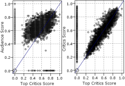
Figure 1: Audience in general have propensity to give high scores with respect to the top critics score. However, average score of critics appears to be more correlated with the score of top critics.

I Introduction

With the growing popularity of the Internet and e-commerce, many new websites have emerged where users can express their opinions about products, such as movies, books, songs, etc. Amazon, for example, stores millions of products that users can search, browse, buy and rate. Consequently, it records millions of hits per day and is one of the most important product websites that has ever existed. Similarly, IMDB lets users get informed about movies and also allows them to read other users’ reviews as well as rate movies themselves.

Most such product rating websites can be modeled as (directed) graphs where users and products are modeled as nodes and the rating of a user for a product is captured by adding a directed edge from the user node to the product node. The graph is bipartite as only users rate products. The weight on the edge captures the “rating” that the user provides to the product. The ratings can be used to rank products as well as recommend them to other users.

Users have inherent bias while rating a product—many users always impart high ratings while many others always rate poorly. For applications in recommendation-based systems where products are ranked according to their ratings, it is important to capture the bias of a user when she is rating a product. In Figure 1, we show the average ratings given to the movies by audience and critics. These ratings are collected from www.rottentomatoes.com and are available as a public dataset. Values on the axes are mostly missing values in the dataset. The website www.rottentomatoes.com also scores the movies by aggregating the reviews from top critics; these scores are deemed more trustworthy. We can observe that audience score is overwhelmingly positive with respect to the top critics score, where as the average score of all the critics is highly correlated with those of top critics. This phenomenon is well observed [2] and is attributed to a difference between quality and user rating. It implies that user ratings have inherent bias and are not trustworthy.

While global ratings (for example, computed as an average of all ratings) are less prone to individual biases of users, individual ratings are susceptible. Many users read the ratings and reviews of other users when trying to decide whether to buy a product or not. Thus, it is necessary to know the bias of a reviewer while reading the review of a product. It is equally important to compensate for this bias while assigning a ranking to an object. It is also observed that for the objects that receive very few ratings, a slight bias on the part of users can lead to a significant change in their ratings [2]. In experiments, we observe such phenomenon as well.

Product ratings usually follow the J-shaped distribution [5], i.e., most of the ratings are overwhelmingly positive along with a small but significant number of high negatives. In Figure 1, we infer similar behavior as well. These ratings do not follow the expected normal distribution. This also indicates that the average rating may not be a right metric to judge product quality because of bias [4, 5]. In this paper we propose a technique which captures user bias and factors it while computing the rating of an object. We follow the intuition that if a user is known to exaggerate her ratings, i.e., user is positively biased, then we compensate for her exaggeration by reducing the ratings. Likewise if a user is known to give low scores, then we increase the ratings.

Specifically, our main contributions are as follows:

1. We propose an iterative technique, where we model both bias and true rating of an item and derive a mutually-recursive formulation.

2. We show that our technique converges to a unique solution, i.e., it does not depend on the initial conditions. Further, we prove that error after any iteration is bounded, and thus, maximum number of iterations required can be fixed apriori.

3. We conduct an in-depth evaluation with the earlier work, current schemes used in the modern system, and more specifically we show that our technique adheres well with the ground truth in terms of absolute error, error in ranking, etc.

4. We also analyze the behavior and error associated with items that receive fewer ratings. We conjectured that such items are likely to be impacted more by user bias. We experimentally verify and analyze this phenomenon in detail.

In section II, we discuss causes of user bias and related approaches for debiasing. In section III, we formally define bias of a user and true rating associated with items. We present the algorithm, its interpretation, iterative technique to compute it, and finally we discuss the complexity of the algorithm. We show the necessary properties such as convergence, uniqueness, and the error-bound in Section IV. In Section V, we give the experimental results such as performance of our algorithm and other approaches (Section V-B), effect of sparse ratings, analysis of ranking, convergence analysis (Section V-C). Finally, we conclude in Section VI.

II Related Work

In this section, we review prior work about the origin of bias and argue that users are indeed biased. We then give a overview of related approaches to compute bias.

II-A Sources of Bias

The bias we usually refer to is known as cognitive bias. It is the human inability to judge the situation based on evidences alone and is influenced by cognitive factors as well. It has been studied in great detail in the area of cognitive science and social psychology. This was introduced by Tversky and Kahneman [6]. In an experiment [12], they presented a numerical estimation of $8!$ (shown in a different manner) to two groups. Two groups came up with a significantly different estimates. When we rely too heavily on few parameters, the bias is known as anchoring bias.

II-B Bias in product ratings

In this subsection, we focus on biases that affects product ratings. First we consider affect heuristic. In general, if a reviewer is presented with large positive ratings and reviews, then she is more likely to give positive scores [11]. Also sorting the reviews based on ratings triggers the affect heuristic as well. Purchasing bias [5] is another example, where people who value a product highly are likely to buy and will not usually write a poor review. Even if we assume that an online rating system (for a user to rate) has been built perfectly including capturing the minute details of an object such as packaging of the object, color, etc., a truthful user may still not conceive it perfectly. For example, it has been observed that user is likely to give high score on Amazon than on eBay [13]. This is because human judgments are subject to a number of bias, including focusing more on few parameters (Amazon emphasizes strength parameter [13]) of the evidence [6].

II-C Existing Approaches

In this section, we review related algorithms proposed to compute bias. In all the algorithms, the main goal was to identify the net bias rather than computing different biases for each user. The first such work [8] noticed that product evaluation depends greatly on the evaluator. They proposed an algorithm to compute bias and showed that it outperforms standard statistical measures. However, their technique looks locally to compute true rating ([8] refer it as consensus), i.e., when source bias is not considered. This will work if these biased ratings can give an unbiased estimate of true rating. However, this is not true. Ranking algorithms like HITS [7] and PageRank [1] look at the global structure, e.g., opinion of a better node should be given more weight. In our case, opinion of a highly biased user should not be directly used to calculate true rating. Recently, [10] proposed many heuristics to compute true ratings based on local approaches. Later, [9] authors improved their existing system by considering the global structure as well. In experiments, we consider this algorithm [9] as the benchmark and give in-depth comparison with our technique.

III Algorithm

The system is modeled as a directed bipartite graph $G=(V=U\cup O,E\subseteq U\times O)$ where $U$ and $O$ denote the set of users and objects (products) respectively. The only edges allowed are those from $U$ to $O$, i.e., users rate objects. Thus, users have only outgoing edges and objects have only incoming edges. We constraint the user to give at most one rating to a product.

The weight of a directed edge, denoted by $w_{ij}$, captures the rating given by user $u_{i}\in U$ to object $o_{j}\in O$. It is assumed that if the weight is high, the user is rating the object positively; on the other hand, if it is low, it is a negative opinion. In this work, we assume the weights to be between $0$ and $1$, i.e., $w_{ij}\in[0,1]$. The neutral rating is somewhere in between, but not necessarily at $0.5$.

The number of edges in such a graph may be large, even if the number of users and objects are not very large. In most real life graph datasets, however, users rate only a few products, and hence, the size of the graph remains within a small factor of the number of nodes.

The standard method to compute the net rating of any item $i$ is to consider the average of all the ratings item $i$ receives ($avg_{j}\{w_{ji}\}$). The method may have some filters such as frequent users, but in general, the mean is considered to be the best estimate. In our work, we aim to remove bias from each individual rating, and then we take the mean. If $f(w_{ji})$ is an estimate of the bias-free rating of a user to a product, then according to our formulation, $avg_{j}\{f(w_{ji})\}$ is the net bias-free rating of the item $i$.

III-A Model

In this section, we precisely define the terms bias of a user $u_{i}$, denoted by $b_{i}$, and true rating of an object $o_{j}$, denoted by $r_{j}$. Further, $d^{+}_{i}$ denotes the set of objects a user $u_{i}$ rates and $d^{-}_{j}$ denotes the set of users that an object $o_{j}$ receives ratings from. Then,

$$\sum_{u_{i}\in U}\left|d^{+}_{i}\right|=\sum_{o_{j}\in O}\left|d^{-}_{j}\right|.$$ (1)

If we know that a user is gives higher ratings than usual, then we expect her ratings to be less trustworthy. In fact, we try to factor in such exaggeration in ratings while coming up with a more realistic rating. We refer to such exaggeration (either high or low) in ratings as bias, and the realistic rating as true rating. In our approach, we compute bias of each user assuming that we know the true ratings of all object. Likewise, we compute true rating of an object by assuming that we know the bias of all object. We create an simple iterative system of two mutually recursive variables, bias and true rating. The precise details are presented next.

III-A1 Bias

The bias of a user is defined as the average deviation of ratings given by her from the true ratings:

$$b_{i}=\frac{1}{\left|d^{+}_{i}\right|}\sum_{o_{j}\in d^{+}_{i}}{\big{(}w_{ij}-r_{j}\big{)}}.$$ (2)

In the above equation, $w_{ij}-r_{j}$ measures the deviation of the user $i$ while rating an object $j$. Here $w_{ij}$ denotes the rating given by the user $i$ to the object $j$, and $r_{j}$ is the true rating of the object $j$. For now, we assume that the true ratings are known. Later, we show that the algorithm converges to a unique solution, irrespective of the initial values of true ratings assumed.

If a user gives higher ratings to objects than the true ratings those objects deserve, the bias of the user will be positive, and the user is said to be positively biased. Such intuition is clearly captured in Eq. (2). Bias of a user can thus be seen as expected exaggeration in her rating an object. Assuming the true ratings also lie between $[0,1]$, the bias values range from $-1$ to $1$, i.e., $b_{i}\in[-1,1]$. If $b_{i}<0$, it means that the user $i$ usually gives lower scores, and likewise if $b_{i}>0$ indicates that the user give higher ratings.

It can be argued that products also have biases, i.e., some products are likely to get high ratings and some are expected to get poor ratings. For example, a good movie is expected to attract high ratings from the viewers. If $\delta$ be the average rating of all the products and $b_{o}$ be the bias of object $o$, then clearly, true rating of the object $o$ is $\delta+b_{o}$. Therefore, the true rating implicitly captures the product bias, and thus we do not have to model item bias separately.

III-A2 True Rating

If we know that the bias of a user, i.e., she gives high/low scores than the average, then we can adjust her rating by factoring in bias. For example, if a user has a positive bias, then her ratings are more than what they should be. Hence, to offset the effect of bias, some fraction of the ratings should be reduced. Similarly, if a user is negatively biased, some fraction of the ratings should be increased. Intuitively, the transformed weight would be the user’s rating minus the bias, i.e., $(w_{ij}-b_{i})$. But this formulation does not guarantee a convergence. Therefore, we make a relaxation to the formulation.

A simple relaxation for a new rating, denoted by $w^{\prime}_{ij}$, after factoring bias can be written as:

$$w^{\prime}_{ij}=w_{ij}-\alpha\cdot b_{i}.$$ (3)

Here we increase the rating, if bias is negative, and decrease if bias is positive. We restrict $\alpha$ to $(0,1)$. For technical reasons, such as convergence, we are forced to keep $\alpha<1$. This will be made clear in later sections. If $\alpha$ is high, we remove more bias and likewise, if $\alpha$ is low, we change the weight by a smaller amount. At the same time, keeping a parameter is also helpful in many situations. For example, if we know that there are few trusted users such as top critics, who are considered as unbiased users. In such a scenario, we can keep $\alpha=0$ for such users. Similarly, if we know that there are few users who are unreliable, then we can keep a high $\alpha$ for such users.

In the above formulation, it should be noted that the new weight can be outside the range $[0,1]$. To overcome this undesirable property, we define a hard cut-off at the boundaries, i.e., $0$ and $1$.

$$w^{\prime}_{ij}=\left\{\begin{array}[]{cl}0&\text{ if }w_{ij}-\alpha\cdot b_{i}\leq 0\\ 1&\text{ if }w_{ij}-\alpha\cdot b_{i}\geq 1\\ w_{ij}-\alpha\cdot b_{i}&\text{ otherwise }\end{array}\right.$$ (7)

This ensures that whenever the new weight is more than $1$, it is reset to $1$ and similarly, whenever it is negative, it is reset to $0$. Eq. (7) can be succinctly written as

$$w^{\prime}_{ij}=\max\big{\{}0,\min\{1,w_{ij}-\alpha\cdot b_{i}\}\big{\}}.$$ (8)

The above function to compute $w^{\prime}_{ij}$ is our de-biasing function (mentioned as $f(\cdot)$ earlier), and it returns the unbiased ratings. Using unbiased ratings, the true rating of an object is defined as the average of the unbiased ratings:

$$r_{j}=\frac{1}{|d^{-}_{j}|}\sum_{u_{i}\in d^{-}_{j}}w^{\prime}_{ij}.$$ (9)

Note that the above definitions, as given in Eq. (2), Eq. (8) and Eq. (9) depend on each other. Later, we show how to solve such a system of interdependent equations using an iterative algorithm.

III-A3 Connection with Co-reference and Co-citation Matrices

We now analyze the bias and true rating formulation using matrix algebra, and see an intriguing connection with the co-reference and co-citation matrices. Notice that there is a non-linearity involved in the formulation of true rating in the form of max and min operators. For simplicity, we ignore these terms in the current section, but later we given an unconditional proof of convergence and uniqueness.

Suppose $\vec{b}$ and $\vec{r}$ are the bias and true rating vectors and $W$ is the adjacency matrix. Let $D^{+}=diag(\left|d^{+}_{1}\right|,\left|d^{+}_{2}\right|,\left|d^{+}_{3}\right|,\ldots)$ and $D^{-}=diag(\left|d^{-}_{1}\right|,\left|d^{-}_{2}\right|,\left|d^{-}_{3}\right|,\ldots)$ be the two diagonal degree matrices. Further, let $C$ be the (symmetric) connection matrix with $0/1$ entries, i.e., if a user rates an item, there is a $1$ entry in the matrix; otherwise, it is $0$. We can now write the bias and true rating vectors as follows:

$$\vec{b} =(D^{+})^{-1}(W\vec{1}-C\vec{r})$$ (10)

$$\vec{r} =(D^{-})^{-1}(W^{T}\vec{1}-\alpha C^{T}\vec{b})$$ (11)

where $(D^{*})^{-1}$ denotes the Moore-Penrose pseudoinverse of the degree matrix.

The analytical solution for bias can be written as:

$$\vec{b} =\left(I-\alpha\cdot(D^{+})^{-1}C(D^{-})^{-1}C^{T}\right)^{-1}\vec{m}$$ (12)

$$=\left(I-\alpha\cdot C^{\prime}C^{{}^{\prime\prime}T}\right)^{-1}\vec{m}$$ (13)

Here, $C^{\prime}$ and $C^{\prime\prime}$ are two degree normalized connection matrices and $\vec{m}=(D^{+})^{-1}(W-C(D^{-})^{-1}W^{T})\vec{1}$. For $(I-\alpha\cdot C^{\prime}C^{{}^{\prime\prime}T})^{-1}$ to exist, we need $\alpha<1$. This constraint on $\alpha$ would ensure that the spectral radius is less than $1$. This is the reason we put a constraint on $\alpha$.

Notice that $C^{\prime}C^{{}^{\prime\prime}T}$ is the co-reference matrix, thus our formulation bears a significant similarity with the Randomized HITS [14], and matrix equations are of similar forms. We can similarly analyze true rating vector which relies on the co-citation matrix.

III-B Iterative algorithm

The iterative algorithm proceeds by updating the bias and rating of nodes in each iteration. Given the bias of users obtained in the previous iteration (say, iteration $t$), the true ratings of objects are computed for the current iteration (i.e., iteration $t+1$). Using these values in turn, the biases are again computed for the current iteration. Denoting the bias of user $u_{i}$ and true rating of object $r_{j}$ at iteration $t$ by $b_{i}^{t}$ and $r_{j}^{t}$ respectively,

$$r_{j}^{t+1} =\frac{1}{|d^{-}_{j}|}\sum_{u_{i}\in d^{-}_{j}}\max\big{\{}0,\min\{1,w_{ij}-\alpha\cdot b^{t}_{i}\}\big{\}}$$ (14)

$$b^{t+1}_{i} =\frac{1}{|d^{+}_{i}|}\sum_{o_{j}\in d^{+}_{i}}\big{(}w_{ij}-r^{t+1}_{j}\big{)}$$ (15)

The above two equations can be combined to obtain a single recursive equation for bias:

$$b^{t+1}_{i} =\frac{1}{|d^{+}_{i}|}\sum_{o_{j}\in d^{+}_{i}}\Big{(}w_{ij}-\frac{1}{|d^{-}_{j}|}\sum_{u_{i}\in d^{-}_{j}}\max\big{\{}0,\min\{1,w_{ij}-\alpha\cdot b^{t}_{i}\}\Big{)}$$

The algorithm proceeds till it reaches the stopping criterion. It may stop when the number of iterations reach a pre-defined threshold or when the change in values of bias and rating fall below another pre-defined threshold. In Section IV-B, we show that the errors fall below a given threshold after at most a certain number of iterations.

The initial bias and rating values are assigned randomly. In Section IV-C, we show that the initial values do not matter, and the final values obtained after convergence of the algorithm are unique.

III-C Complexity

We now analyze the runtime complexity of the above iterative algorithm. In each iteration, the values of bias and rating are updated for all nodes. Updating the rating of an object $o_{j}$ requires $O(|d^{-}_{j}|)$ time. For all objects, the amortized total time taken is $O(\sum_{o_{j}}|d^{-}_{j}|)=O(m)$, where $m$ is the number of edges in the graph. Similarly, updating the bias of user $u_{i}$ requires $O(|d^{+}_{i}|)$ time. The amortized total time taken for all users is $O(\sum_{u_{i}}|d^{+}_{i}|)$ which is again $O(m)$. Thus, the time spent per iteration is $O(m)$. If the algorithm is run for $k$ iterations, the total running time is $O(km)$.

Although $m$ can be as large as $|U|\cdot|O|$, for most practical datasets, the users rate only a handful of objects. Hence, in practice, $m\ll|U|\cdot|O|$. In general, $m$ is more close to $n=O(\max\{|U|,|O|\})$. We show in Section IV-B that the number of iterations $k$ is logarithmic in the (inverse) error term. Thus, the algorithm is very fast.

IV Properties of the algorithm

In this section, we characterize certain useful properties of the algorithm including error bounding of values and convergence to unique values. In this section, we show that error after any iteration is bounded. This helps in fixing the maximum number of required iterations apriori. Before we proceed to the proof, we present four facts. Namely

Fact 1: If $w-\alpha\cdot b_{i}\geq 1\implies$ $\max(0,\min(1,w-\alpha\cdot b_{i}))=1.$
Fact 2: If $w-\alpha\cdot b_{i}\leq 0\implies$ $\max(0,\min(1,w-\alpha\cdot b_{i}))=0.$
Fact 3: If $0\leq(w-\alpha\cdot b_{i})\leq 1\implies$ $\max(0,\min(1,w-\alpha\cdot b_{i}))=(w-\alpha\cdot b_{i})$.
Fact 4: $|b_{i}^{*}-b_{j}^{*}|\leq 2$.

We now prove the following lemma that states that the difference between the ratings are bounded by the difference between the different values of bias. It is used in later proofs.

Lemma 1

Suppose $b^{m}_{i}$ and $b^{n}_{i}$ are two values of bias of node $i$. These can be the values in two different iterations $m$ and $n$ or can also be two different biases when the initial conditions are different, i.e., we start with two different seed values of bias. We prove the following inequality:

$$M =|\max(0,\min(1,w-\alpha\cdot b^{m}_{i})-\max(0,\min(1,w-\alpha\cdot b^{n}_{i})|$$

$$\leq\alpha\cdot|b^{m}_{i}-b^{n}_{i}|$$

Proof:

We prove this for six possible cases:

1. When $(w-\alpha\cdot b^{m}_{i})\geq 1$ and $(w-\alpha\cdot b^{n}_{i})\geq 1$:
   Using Fact 1 we can observe that $M=0$. Since both $\alpha$ and $|b^{m}_{i}-b^{n}_{i}|$ are positive quantities, we can represent this in an inequality form as $M\leq\alpha\cdot|b^{m}_{i}-b^{n}_{i}|$.

2. When $(w-\alpha\cdot b^{m}_{i})\geq 1$ and $0\leq(w-\alpha\cdot b^{n}_{i})\leq 1$:
   Using Fact 1, we get $M=1-(w-\alpha\cdot b^{n}_{i})$. We know that $(w-\alpha\cdot b^{m}_{i})\geq 1$. Therefore, $M\leq((w-\alpha.b^{m}_{i})-(w-\alpha\cdot b^{n}_{i}))$. Hence $M\leq\alpha\cdot|b^{m}_{i}-b^{n}_{i}|$.

3. When $(w-\alpha\cdot b^{m}_{i})\geq 1$ and $(w-\alpha\cdot b^{n}_{i})\leq 0$:
   From Fact 1 and Fact 2, we get $M=1$. Since $(w-\alpha\cdot b^{m}_{i})\geq 1$ and $(w-\alpha\cdot b^{n}_{i})\leq 0$, $\alpha\cdot|b^{m}_{i}-b^{n}_{i}|\geq 1$. Therefore $M\leq\alpha\cdot|b^{m}_{i}-b^{n}_{i}|$.

4. When $0\leq(w-\alpha\cdot b^{m}_{i})\leq 1$ and $0\leq(w-\alpha\cdot b^{n}_{i})\leq 1$:
   Using Fact 3, we obtain $M=(w-\alpha\cdot b^{m}_{i})-(w-\alpha\cdot b^{n}_{i})=\alpha.|b^{m}_{i}-b^{n}_{i}|$. In other words, $M\leq\alpha\cdot|b^{m}_{i}-b^{n}_{i}|$.

5. When $0\leq(w-\alpha\cdot b^{m}_{i})\leq 1$ and $(w-\alpha\cdot b^{n}_{i})\leq 0$:
   Using Fact 3 and Fact 2, we get $M=(w-\alpha\cdot b^{m}_{i})$. Now, let us consider a quantity $N=|(w-\alpha\cdot b^{m}_{i})-(w-\alpha\cdot b^{n}_{i})|$. Since, $(w-\alpha\cdot b^{n}_{i})\leq 0$, therefore, $N=|(w-\alpha\cdot b^{m}_{i})|+|(w-\alpha\cdot b^{n}_{i})|$. Notice that $N\geq M$ and we can rewrite $N$ as $\alpha\cdot|b^{m}_{i}-b^{n}_{i}|$. Therefore, $M\leq\alpha\cdot|b^{m}_{i}-b^{n}_{i}|$.

6. When $(w-\alpha\cdot b^{m}_{i})\leq 0$ and $(w-\alpha\cdot b^{n}_{i})\leq 0$:
   Using Fact 2, we get $M=0$. Since $\alpha\cdot|b^{m}_{i}-b^{n}_{i}|$ is a positive quantity, therefore, $M\leq\alpha\cdot|b^{m}_{i}-b^{n}_{i}|$.

∎

IV-A Error-bound

In this section, we bound the error; specifically, we show that the difference of bias of two consecutive iterations is bounded and it decreases exponentially as we increase the number of iterations.

Suppose $b^{t}_{i}$ is the bias value of node $i$ after $t$ iterations. We prove the following theorem on error that states that the difference is bounded by an exponential factor of $\alpha$.

Theorem 1

The difference of bias of a node at any iteration $t$ from the next iteration is bounded by an inverse exponential function of $t$:

$$|b^{t+1}_{i}-b^{t}_{i}|\leq{2\cdot\alpha^{t+1}}.$$ (16)

Proof:

We use mathematical induction for the proof. Basis: We first prove for $t=0$.

$$|b^{1}_{i}-b^{0}_{i}|$$

$$=\Big{|}\frac{1}{|d^{+}_{i}|}\sum_{j\in d^{+}_{i}}\Big{(}\frac{1}{|d^{-}_{j}|}\sum_{k\in d^{-}_{j}}\Big{(}\max(0,\min(1,w_{kj}-\alpha\cdot b^{1}_{k}))$$

$$\qquad\qquad-\max(0,\min(1,w_{kj}-\alpha\cdot b^{0}_{k}))\Big{)}\Big{)}\Big{|}$$

$$\leq\Big{|}\frac{1}{|d^{+}_{i}|}\sum_{j\in d^{+}_{i}}\Big{(}\frac{1}{|d^{-}_{j}|}\sum_{k\in d^{-}_{j}}\Big{|}\max(0,\min(1,w_{kj}-\alpha\cdot b^{1}_{k}))$$

$$\qquad\qquad-\max(0,\min(1,w_{kj}-\alpha\cdot b^{0}_{k}))\Big{|}\Big{)}\Big{|}$$

$$\leq\left|\frac{1}{|d^{+}_{i}|}\sum_{j\in d^{+}_{i}}\left(\frac{1}{|d^{-}_{j}|}\sum_{k\in d^{-}_{j}}(\alpha\cdot|b^{2}_{k}-b^{1}_{k}|)\right)\right|\mbox{ [Using Lemma 1]}$$

$$\leq\left|\frac{1}{|d^{+}_{i}|}\sum_{j\in d^{+}_{i}}\left(\frac{1}{|d^{-}_{j}|}\sum_{k\in d^{-}_{j}}(\alpha\cdot 2)\right)\right|\leq 2\cdot\alpha\qquad\mbox{[Using Fact 4]}$$

Induction step: We assume the bound to be true for $b^{t}_{i}$ in the $t^{\text{th}}$ iteration, i.e., $b^{t}_{i}-b^{t-1}_{i}\leq 2\cdot\alpha^{t}$. In the $(t+1)^{\text{th}}$ iteration,

$$|b^{t+1}_{i}-b^{t}_{i}|$$

$$=\Big{|}\frac{1}{2|d^{+}_{i}|}\sum_{j\in d^{+}_{i}}\Big{(}\frac{1}{|d^{-}_{j}|}\sum_{k\in d^{-}_{j}}\max(0,\min(1,w_{kj}+\alpha\cdot b^{t}_{k}))$$

$$\qquad\qquad-\max(0,\min(1,w_{kj}+\alpha\cdot b^{t-1}_{k})))\Big{)}\Big{|}$$

$$\leq\left|\frac{1}{|d^{+}_{i}|}\sum_{j\in d^{+}_{i}}\left(\frac{1}{|d^{-}_{j}|}\sum_{k\in d^{-}_{j}}(\alpha\cdot|b^{t}_{k}-b^{t-1}_{k}|)\right)\right|$$

$$\leq\left|\frac{1}{|d^{+}_{i}|}\sum_{j\in d^{+}_{i}}\left(\frac{1}{|d^{-}_{j}|}\sum_{k\in d^{-}_{j}}(\alpha\cdot 2\cdot(\alpha)^{t})\right)\right|\quad\mbox{[Induction assumption]}$$

$$=2\cdot\alpha^{t+1}$$

Thus, the error is bounded by an inverse exponential function of $t$. ∎

IV-B Proof of Convergence

Using the above error bounds, we can observe that difference of two consecutive iterations decrease as we increase the number of iterations. For any $\epsilon>0$, we have $t=\log_{1/\alpha}(\frac{2}{\epsilon})$ such that for any two iterations $m,n>t$, we have:

$$|b^{m}-b^{n}|\leq\epsilon$$

The above sequence is a Cauchy sequence and thus converges.

IV-C Proof of Uniqueness

We next establish the proof for the uniqueness of the system. We will prove it by contradiction. Assume that there are at least two values of bias that satisfy the bias equation. Suppose $b^{1}_{i}$ and $b^{2}_{i}$ be two converged values of node $i$ and their difference is $\delta(i)=b^{1}_{i}-b^{2}_{i}$. Suppose, $M$ denotes the largest such difference, i.e., $M=\max_{i}\delta(i)$. If we can show that $M$ is zero, then uniqueness is proved. In other words, there exist a single solution to the bias equation.

Theorem 2

The bias of a node converges to a unique value.

Proof:

$$M=\Big{|}\frac{1}{2|d^{+}_{i}|}\sum_{j\in d^{+}_{i}}\Big{(}\frac{1}{|d^{-}_{j}|}\sum_{k\in d^{-}_{j}}\max(0,\min(1,w_{kj}-\alpha\cdot b^{1}_{k}))$$

$$\qquad\qquad\qquad-\max(0,\min(1,w_{kj}-\alpha\cdot b^{2}_{k}))\Big{)}\Big{|}$$

$$\leq\Big{|}\frac{1}{|d^{+}_{i}|}\sum_{j\in d^{+}_{i}}\Big{(}\frac{1}{|d^{-}_{j}|}\sum_{k\in d^{-}_{j}}\Big{|}\max(0,\min(1,w_{kj}-\alpha\cdot b^{1}_{k}))$$

$$\qquad\qquad\qquad-\max(0,\min(1,w_{kj}-\alpha\cdot b^{2}_{k}))\Big{|}\Big{)}\Big{|}$$

$$\leq\left|\frac{1}{|d^{+}_{i}|}\sum_{j\in d^{+}_{i}}\left(\frac{1}{|d^{-}_{j}|}\sum_{k\in d^{-}_{j}}(\alpha\cdot|b^{1}_{k}-b^{2}_{k}|)\right)\right|\mbox{[Using Lemma 1]}$$

$$\leq\left|\frac{1}{|d^{+}_{i}|}\sum_{j\in d^{+}_{i}}\left(\frac{1}{|d^{-}_{j}|}\sum_{k\in d^{-}_{j}}(\alpha\cdot|b^{1}_{p}-b^{2}_{p}|)\right)\right|\mbox{[By definition ]}$$

$$=\left|\frac{1}{|d^{+}_{i}|}\sum_{j\in d^{+}_{i}}\left(\frac{1}{|d^{-}_{j}|}\sum_{k\in d^{-}_{j}}(\alpha\cdot M)\right)\right|$$

$$=\alpha\cdot M$$

Since $\alpha\leq 1$ and M is a positive quantity, inequality $M\leq\alpha\cdot M$ holds when $M=0$. This confirms uniqueness. ∎

Bin	Number of ratings	Count of movies
		Dataset 1	Dataset 2
1	1	114	13
2	2-3	131	26
3	4-7	142	40
4	8-15	204	76
5	16-31	311	109
6	32-63	463	216
7	64-127	508	258
8	128-255	633	363
9	256-511	598	366
10	512-1023	406	273
11	$>$1023	196	122
	Total	3706	1862

TABLE I: Grouping of movies based on the number of ratings received.

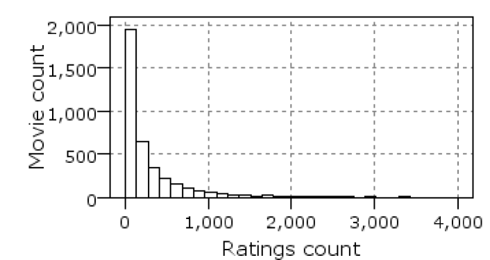
Figure 2: Distribution of number of movies with number of ratings received for Dataset 1. Most movies received very few ratings.

V Experiments

V-A Dataset description

We use two datasets for our experiments. They are available from http://www.grouplens.org. The first dataset from www.grouplens.org/node/73 consists of roughly 1 million movie ratings given by around 6,000 users to around 3,700 movies. The second dataset from http://www.grouplens.org/node/462 contains extra information about the movies such as ratings given by the top critics. Thus we have both user ratings and the net score given by the top critics. We call the first dataset as Dataset 1 and the second dataset as Dataset 2 throughout the paper.

In both the datasets, most of the movies receive only a few ratings. For example, in Figure 2, we show the histogram of movies over the number of ratings they receive for Dataset 1. We can notice that movies with few ratings dominates the set. In Dataset 2, we observe similar behavior as it is essentially a subset of Dataset 1 with extra information such as top critics ratings. To gain more insights, we divide the two datasets into different bins based on the number of ratings a movie receive. This helps in analyzing the rating data in much greater detail. We divided all the movies in 11 groups (or bins) based on the number of ratings they receive. While binning, we particularly focused on those movies which received fewer ratings. Table I shows the distribution. In both these datasets, we normalize the movie ratings in the range $0$ to $1$, with $0$ implying the lowest score and $1$ the highest.

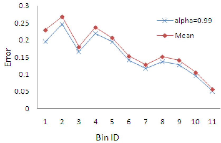
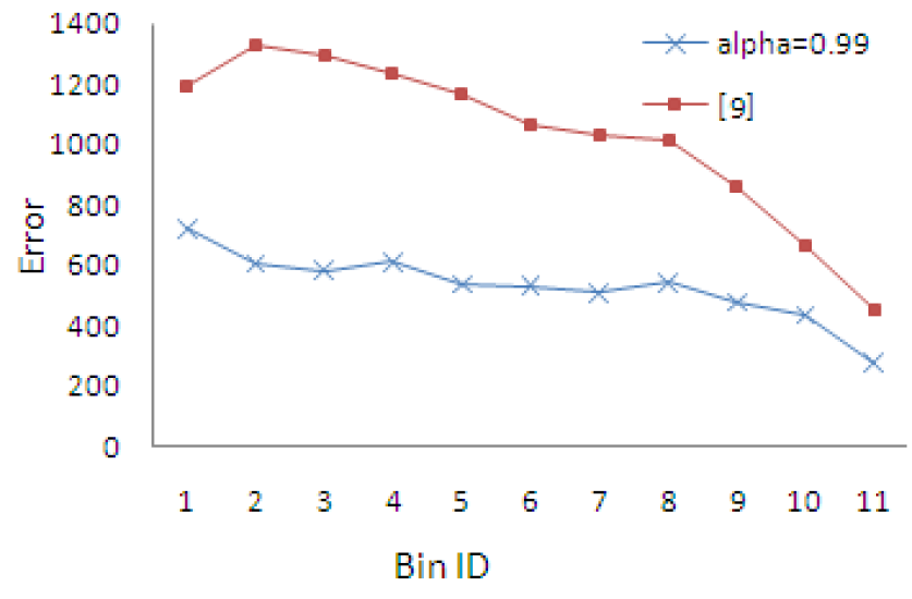
Figure 3: Mean Square Error for techniques on the Dataset 2.

Figure 4: Absolute error in ranking computed over the Dataset 2.

V-B Performance Evaluation

In this section, we report the results against the baseline and existing techniques. Later (Section V-C) we analyze the behavior of our algorithm qualitatively.

We consider the top critics rating as the ground truth, and we compare the various techniques against this metric. We compute the mean square error (MSE) and error in ranking. In MSE, we simply look at the deviation in ratings returned by different techniques with respect to the top critics rating. It has been shown that the critics score correlate well with the box office success of a movie in a long term, not so much with early box office receipts [3]. Therefore, it is fit to serve as a ground truth. To the best of our knowledge, Dataset 2 is the only publicly available dataset with critics ratings, and therefore in this set of experiments, we use this dataset alone.

We show that our algorithm adheres well with the critics’ rating than the baseline method and a representative algorithm [9]. Mean rating is currently the most widely used approach in most systems with small filtering mechanisms such as frequent users. Therefore, it is a good candidate for a baseline. The algorithm in [9], similar to our algorithm, exploits the global structure of the graph rather than focusing locally. The original algorithm suffers from the divide-by-zero problem and the authors suggested using a small value; so, for our comparison, we used $0.01$.

Note that the algorithm proposed in [9] does not converge and the final values (which are out of scale) depend on the initial seeds. For a fair comparison with this algorithm, we consider another metric—error in ranking. Initially, we sort the movies based on the top critics score to know their ranks and then we simply look at the average absolute distance between the ranking returned by the technique (our algorithm and [9]) and critics ranking.

The mean square error with mean rating on Dataset 2 is $0.142$ while our algorithm ($\alpha=0.99$) reduces it to $0.129$. In later sections, we analyze the behavior of our algorithm for different values of $\alpha$. For now, we assume that we are trying to remove as much bias as possible, and therefore, we keep a high value for $\alpha$ (such as $0.99$). To gain more insight, we plot the error across different bins Table I for these two techniques in Figure 4. We can observe that our algorithm gives superior results across all the bins, especially in the ones that receive few ratings. We can also observe that the error reduces as the number of ratings per bin increases. This phenomenon is explained in detail in Section V-C2.

Algorithm proposed in [9] does not converge, therefore we compare the ranking returned by our algorithm against those as authors [9] originally suggested. In Figure 4, we can notice that our algorithm outperforms the algorithm. Also, the error in ranking decreases as the number of ratings increases.

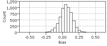
(a) Bias distribution for $\alpha=0.99$.

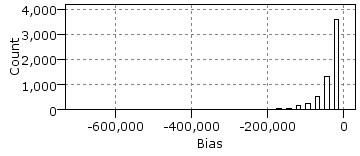
(b) Bias distribution for [9].

Figure 5: Distribution of bias.

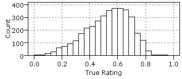
(a) True rating distribution for $\alpha=0.99$.

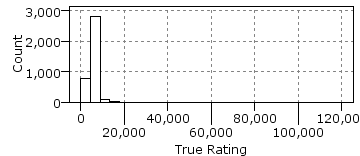
(b) True rating distribution for [9].

Figure 6: Distribution of true ratings.

V-C Qualitative Evaluation

In this section, we look at other properties of our algorithm, mean rating and the algorithm proposed in [9] such as the distribution of bias, effect of number of ratings a movie receives, convergence analysis of the algorithm, and comparison of relative rankings. As Dataset 2 is simply a smaller subset of Dataset 1 with the additional critics information, we now show results directly on the Dataset 1.

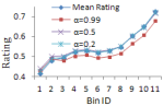
(a) Variation of ratings across bins.

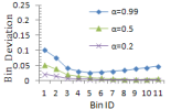
(b) Deviation of ratings across bins.

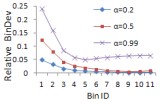
(c) Relative deviation of ratings across bins.

Figure 7: Comparison of ratings across different bins.

V-C1 Distribution of bias and true rating

In this experiment, we look at the distribution of bias and true rating obtained by running our algorithm and algorithm in [9]. Figure 5 shows the distribution of bias at the end of $10$ iterations. Our algorithm gives a bell curve type distribution. Note that the algorithm in [9] did not converge. We observed small changes in the bias distribution for different values of $\alpha$ such as $0.2$, $0.5$ and $0.99$. The bias values obtained by the algorithm in [9] are all negative and out of scale. Our bias values, on the other hand, quantify the effect by which the rankings etc. are shifted, and are therefore, more close to actual biases.

Figure 6(b) shows similar distribution of true ratings at the end of $10$ iterations for our method and the algorithm in [9]. Even with high $\alpha$ our algorithm gives meaningful value of true rating. Once again, the actual values of true ratings obtained using the algorithm in [9] are useful only for relative ranking purposes and the absolute values do not convey anything. The ratings obtained by our method are more indicative of the actual ratings.

V-C2 Effect of number of ratings

As discussed earlier, there are many movies for which the number of ratings is quite less. There are many reasons for fewer ratings. A movie that has been marked as “poor” by a user is likely to be watched by less number of people and will thus have only a few ratings. On the other hand, when a movie is rated “excellent”, more people watch/buy it, and the movie receives more ratings. This behavior is loosely termed as purchasing bias. Thus, we expect a movie with a large number of reviews to have high ratings, and a movie which is rated by few users to be lowly rated in general. Experiments also reveal such behavior.

Figure 7(a) shows the variation of the true ratings obtained using different $\alpha$ values. It also plots the mean of the original ratings. As predicted by the purchasing bias, movies with more ratings generally have higher values. We did not plot the ratings obtained using the algorithm in [9], as they are very high and out of scale and their absolute values do not signify anything. Instead, later we compare with the relative ranking as the authors in [9] intend to do.

The next graph, Figure 7(b), plots the deviations for each bin. It captures the average difference of the true ratings from the mean rating. The deviation of bin $k$ is

$$bindev(k)=\frac{1}{|bin(k)|}\sum_{o_{j}\in bin(k)}|r_{j}-meanRating_{j}|$$

where $|bin(k)|$ is the number of movies in bin $k$ and $meanRating_{j}$ is the mean rating of movie $o_{j}$.

The deviation is high for movies that receive fewer ratings and is much low for movies that are rated by many users. This can be explained by the “law of large numbers” that states that the average of a large number of values is closer to the expected value. The second important observation is the fact that the deviation is higher for larger $\alpha$. The parameter $\alpha$ denotes the quantity that is removed from the mean rating. When $\alpha=0$, the user is never biased, and the true rating is equal to the mean rating. With a larger amount of shift, the deviation is larger as well. Finally, it seems that the deviation in later bins (those with more ratings) are higher. It is because average true rating also increases in the later bins. However, we do not expect the relative deviation to be as large.

To understand this behavior better, we next compute the relative deviation in each bin as the ratio of deviation to the true rating:

$$relbindev(k)=\frac{1}{|bin(k)|}\sum_{o_{j}\in bin(k)}\frac{|r_{j}-meanRating_{j}|}{r_{j}}$$

Figure 7(c) shows the graph.

Indeed, the relative deviations in bins with fewer ratings are much higher. While for movies having less than 4 ratings, the relative deviation can be as high as 25% , for those with more ratings, it stabilizes to 1%. Even when $\alpha$ is very high ($0.99$), it is around 5% only.

Movie ID	Mean	$\alpha=$			[9]
	Rating	$0.2$	$0.5$	$0.99$
3280	1	12	101	1417	4
3233	2	3	3	4	2021
1830	3	7	7	9	19
3881	4	9	10	33	1641
3656	5	8	8	15	2688
787	6	5	5	5	1152
3607	7	6	6	10	10
3172	8	4	4	6	3456
3382	9	1	1	1	1
989	10	2	2	3	3369

TABLE II: Top ranked movie and their IDs upon sorting by mean rating.

Movie ID	$\alpha=$			Mean	[9]
	$0.99$	$0.2$	$0.5$	Rating
3282	1	1	1	9	1
557	2	15	9	23	5
989	3	2	2	10	3369
3233	4	3	3	2	2021
787	5	5	5	6	1152
3172	6	4	4	8	3456
578	7	17	14	25	9
2503	8	13	13	13	34
1830	9	7	7	3	19
3607	10	6	6	7	10

TABLE III: Top ranked movie and their IDs upon sorting by true rating for $\alpha=0.99$.

Movie ID	$\alpha=$			Mean	[9]
	$0.2$	$0.5$	$0.99$	Rating
2858	79	91	111	76	209
260	35	35	50	34	208
1196	98	108	149	91	318
1210	377	407	486	345	616
480	889	936	1016	861	1080
2028	67	77	107	64	316
589	320	354	417	300	594
2571	82	96	126	77	205
1270	429	455	529	438	838
593	60	62	76	60	277

TABLE IV: Movie are sorted (descending) based on the number of ratings they received.

Movie ID	$\alpha=$			Mean	[9]
	$0.2$	$0.5$	$0.99$	Rating
127	3674	3634	3225	3678	3686
133	3670	3544	2355	3679	3696
139	450	529	709	374	3555
142	3696	3691	3687	3684	3688
226	3529	3536	3573	3520	3551
286	2369	2145	1727	2464	94
311	2358	2112	1652	2466	3477
396	440	503	654	376	38
398	366	333	286	377	3380
402	2400	2216	1857	2543	37

TABLE V: Movies which received only $1$ vote.

V-C3 Comparison of relative ratings

A ranked solution has also been proposed by the authors of [9]. They have shown that relative ranking could still be preserved even if the algorithm does not converge. In this section, we compare the ranking of movies based on the ratings obtained using the algorithm in [9] and our algorithm.

The first table, Table V, ranks the movies according to the mean rating they received originally. When $\alpha$ is small, there is little effect of bias, and our rankings closely resemble that of mean rating. In general, we do not expect a movie with a high mean rating to become a very bad movie after removing bias. There will be some difference and as $\alpha$ increases, such differences may increase. Still, we do not expect a dramatic change. Even for very large $\alpha$ ($0.99$), the list obtained is better than that using [9]. Many of the top-10 movies in that list are ranked in thousands as opposed to only one such case for our algorithm. In general, our results are more stable.

In the next table, Table V, we first sort the movies according to the ratings obtained using $\alpha=0.99$, and then tabulate their rankings using the other schemes. Once more it can be observed that all the ranked lists are similar except for the algorithm in [9] as it shows instabilities.

Movies that are rated by many users generally receive higher ratings. In Table V, movies are sorted in a descending order according to the number of ratings they have received. Most largely rated movies are indeed highly rated. All the algorithms including the one from [9] rank them high (within 15%, but mostly within 10%).

It is, however, more interesting to analyze how the rankings behave for movies that receive very few ratings. The final table, Table V, show the results for movies that have received only a single vote. We have shown only 15 movies sorted according to their IDs. As indicated by the purchasing bias, these movies are poorly rated, both according to mean rating and our algorithm. The algorithm in [9], shows some inconsistent results and ranks certain poorly rated movies very highly (e.g., movie IDs 286, 396, and 402). Our algorithms show more meaningful and stable ranking.

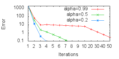
(a) True Rating.

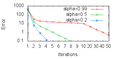
(b) Bias.

Figure 8: Convergence plot: error versus number of iterations.

V-C4 Convergence

In this set of experiments, we empirically measure the rate at which our algorithm converges. Figure 8 shows the rate of convergence for both true rating and bias. The error is measured as the sum of differences in bias (or true rating) values over all nodes between two consecutive iterations. The algorithm in [9] did not converge in our setting.

We choose $0$ as the initial seed value of bias for all nodes. In the first iteration, this value is used to compute true ratings and in turn the new bias values. Since seed bias is $0$, bias computation is independent of $\alpha$ for first iteration. From second iteration onward, $\alpha$ starts to make a difference in the convergence rate of bias and true rating.

In the graphs, we have plotted the error values up to 50 iterations. We use the $L_{1}$ norm to compute error. Note that an error value, say $0.1$, as shown in the graph is the sum of error values over 3,000 nodes. Consequently, the error for a single node is very low.

The rate of convergence is slower for a larger $\alpha$. When $\alpha\to 1$, the error in each node can be as large, and therefore, the rate of convergence will be slow. On the other hand, for a small $\alpha$, the values converge very rapidly, and the algorithm is very practical.

Since it has been shown that the error falls exponentially, the stopping criterion can also be chosen to be when the difference in values between two consecutive iterations becomes less than a threshold $\epsilon$. The number of iterations is a logarithmic function in the inverse of the threshold $\epsilon$.

VI Conclusion

In this work, we have proposed a novel technique to compute the bias of users and consequently true ratings for products. People have different views when they rate a product and it is necessary to capture their bias. By factoring bias, we obtain true ratings of a product. The bias and true rating values computed by our algorithm are meaningful and can be associated directly with the ratings user provide. Our algorithm is iterative, fast and has several nice properties including convergence to a unique solution and bounded errors. The maximum number of required iteration can also be fixed apriori depending on the level of accuracy required. In experiments, we observe that our technique produces consistent and good results. In future, we would like to analyze the change in user biases over time. For example, users tend to give high ratings right after a movie release.

References

- [1] S. Brin and L. Page. The anatomy of a large-scale hypertextual web search engine. In WWW, pages 107–117, 1998.
- [2] B.-C. Chen, J. Guo, B. Tseng, and J. Yang. User reputation in a comment rating environment. In KDD, pages 159–167, 2011.
- [3] J. Eliashberg and S. M. Shugan. Film Critics: Influencers or Predictors? The Journal of Marketing, 61(2):68–78, 1997.
- [4] N. Hu, P. A. Pavlou, and J. Zhang. Can online reviews reveal a product’s true quality?: empirical findings and analytical modeling of online word-of-mouth communication. In EC, pages 324–330, 2006.
- [5] N. Hu, J. Zhang, and P. A. Pavlou. Overcoming the j-shaped distribution of product reviews. Commun. ACM, 52(10):144–147, 2009.
- [6] D. Kahneman and A. Tversky. Judgment under uncertainty: Heuristics and biases. Cognitive Psych., 3:430–454, 1972.
- [7] J. M. Kleinberg. Authoritative sources in a hyperlinked environment. In SODA, pages 668–677, 1998.
- [8] H. W. Lauw, E.-P. Lim, and K. Wang. Bias and controversy: beyond the statistical deviation. In KDD, pages 625–630, 2006.
- [9] H. W. Lauw, E.-P. Lim, and K. Wang. Summarizing review scores of ”unequal” reviewers. In SDM, 2007.
- [10] M. McGlohon, N. S. Glance, and Z. Reiter. Star quality: Aggregating reviews to rank products and merchants. In ICWSM, 2010.
- [11] D. Pothier and D. Carlson. Cognitive bias in online open systems:examining relevant heuristics and cognitive biases in open systems on the internet. Knol, Version 17, 2010. Available at http://knol.google.com/k/dan/cognitive-bias-in-online-open-systems/bbftwjxfm1vs/3.
- [12] A. Tversky and D. Kahneman. Judgment under uncertainty: Heuristics and biases. Science, 185(4157):1124–1131, Sept. 1974.
- [13] J. R. Wolf and W. A. Muhanna. Feedback mechanisms, judgment bias and trust formation in online auctions. Decision Sciences, 42:43–68, 2011.
- [14] A. X. Zheng, A. Y. Ng, and M. I. Jordan. Stable algorithms for link analysis. In SIGIR, pages 258–266, 2001.