Fast calculation of inverse square root with the use of magic constant – analytical approach

Abstract

We present a mathematical analysis of transformations used in fast calculation of inverse square root for single-precision floating-point numbers. Optimal values of the so called magic constants are derived in a systematic way, minimizing either absolute or relative errors at subsequent stages of the discussed algorithm.

Keywords: floating-point arithmetics; inverse square root; magic constant; Newton-Raphson method

1 Introduction

Floating-point arithmetics has became wide spread in many applications such as 3D graphics, scientific computing and signal processing [1, 2, 3]. Basic operators such as addition, subtraction, multiplication are easier to design and yield higher performance, high throughput but advanced operators such as division, square root, inverse square root and trigonometric functions consume more hardware, slower in performance and slower throughput [4, 5, 6, 7, 8].

Inverse square root function is widely used in 3D graphics especially in lightning reflections [9, 10, 11]. Many algorithms can be used to approximate inverse square root functions [12, 13, 14, 15, 16]. All of these algorithms require initial seed to approximate function. If the initial seed is accurate then iteration required for this function is less time-consuming. In other words, the function requires less cycles. In most of the case, initial seed is obtained from Look-Up Table (LUT) and the LUT consume significant silicon area of a chip. In this paper we present initial seed using so called magic constant [17, 18] which does not require LUT and we then used this magic constant to approximate inverse square root function using Newton-Raphson method and discussed its analytical approach.

We present first mathematically rigorous description of the fast algorithm for computing inverse square root for single-precision IEEE Standard 754 floating-point numbers (type float).

1.	float InvSqrt(float x){
2.		float halfnumber = 0.5f * x;
3.		int i = *(int*) &x;
4.		i = R-(i$>>$1);
5.		x = *(float*)&i;
6.		x = x*(1.5f-halfnumber*x*x);
7.		x = x*(1.5f-halfnumber*x*x);
8.		return x ;
9.	}

This code, written in C, will be referred to as function InvSqrt. It realizes a fast algorithm for calculation of the inverse square root. In line 3 we transfer bits of varaible x (type float) to variable i (type int). In line 4 we determine an initial value (then subject to the iteration process) of the inverse square root, where $R=0x5f3759df$ is a “magic constant”. In line 5 we transfer bits of a variable i (type int) to the variable x (type float). Lines 6 and 7 contain subsequent iterations of the Newton-Raphson algoritm.

The algorithm InvSqrt has numerous applications, see [19, 20, 21, 22, 23]. The most important among them is 3D computer graphics, where normalization of vectors is ubiquitous. InvSqrt is characterized by a high speed, more that 3 times higher than in computing the inverse square root using library functions. This property is discussed in detail in [24]. The errors of the fast inverse square root algorithm depend on the choice of $R$. In several theoretical papers [18, 24, 25, 26, 27] (see also the Eberly’s monograph [9]) attempts were made to determine analytically the optimal value (i.e. minimizing errors) of the magic constant. These attempts were not fully successfull. In our paper we present missing mathematical description of all steps of the fast inverse square root algorithm.

2 Preliminaries

The value of a floating-point number can be represented as:

$$x=(-1)^{s_{x}}(1+m_{x})2^{e_{x}},$$ (2.1)

where $s_{x}$ is the sign bit ($s_{x}=1$ for negative numbers and $s_{x}=0$ for positive numbers), $1+m_{x}$ is normalized mantissa (or significand), where $m_{x}\in\langle 0,\;1)$ and, finally, $e_{x}$ is an integer.

In the case of the standard IEEE-754 a floating-point number is encoded by $32$ bits (Fig. 1). The first bit corresponds to a sign, next $8$ bits correspond to an exponent $e_{x}$ and the last $23$ bits encodes a mantissa. The fractional part of the mantissa is represented by an integer (without a sign) $M_{x}$:

$$M_{x}=N_{m}\,m_{x},\quad\quad\text{where: \ $N_{m}=2^{23}$},$$ (2.2)

and the exponent is represented by a positive value $E_{x}$ resulting from the shift of $e_{x}$ by a constant $B$ (biased exponent):

$$E_{x}=e_{x}+B,\quad\quad\text{where: \ $B=127$}.$$ (2.3)

Bits of a floating-point number can be interpreted as an integer given by:

$$I_{x}=(-1)^{s_{x}}(N_{m}\,E_{x}+M_{x}),$$ (2.4)

where:

$$M_{x}=N_{m}(2^{-e_{x}}x-1)$$ (2.5)

Figure 1: The layout of a 32-bit floating-point number.

In what follows we confine ourselves to positive numbers ($s_{x}\equiv b_{S}=0$). Then, to a given integer $I_{x}\in\langle 0,2^{32}-1\rangle$ there corresponds a floating number $x$ of the form (2.1), where

$$e_{x}:=\lfloor N_{m}^{-1}I_{x}\rfloor-B\ ,\qquad m_{x}:=N_{m}^{-1}I_{x}-\lfloor N_{m}^{-1}I_{x}\rfloor\ .$$ (2.6)

This map, denoted by $f$, is inverse to the map $x\rightarrow I_{x}$. In other words,

$$f(I_{x})=x\ .$$ (2.7)

The range of available 32-bit floating-point numbers for which we can determine inverse square roots can be divided into 127 disjoint intervals:

$$x\in\bigcup_{n=-63}^{63}A_{n},\quad\text{where: $A_{n}=\{2^{2n}\}\cup\underbrace{(2^{2n},2^{2n+1})}_{A_{n}^{I}}\cup\langle\underbrace{2^{2n+1},2^{2(n+1)})}_{A_{n}^{II}}$}.$$ (2.8)

Therefore, $e_{x}=2n$ for $x\in A^{I}_{n}\cup\{2^{2n}\}$ and $e_{x}=2n+1$ for $x\in A^{II}_{n}$. For any $x\in A_{n}$ exponents and significands of $y=1/\sqrt{x}$ are given by

$$e_{y}=\left\{\begin{array}[]{cl}-n&\text{for $x=2^{2n}$}\\ -n-1&\text{for $x\in A_{n}^{I}$}\\ -n-1&\text{for $x\in A_{n}^{II}$}\end{array}\right.,\quad m_{y}=\left\{\begin{array}[]{cl}0&\text{for $x=2^{2n}$}\\ 2/\sqrt{1+m_{x}}-1&\text{for $x\in A_{n}^{I}$}\\ \sqrt{2}/\sqrt{1+m_{x}}-1&\text{for $x\in A_{n}^{II}$}\end{array}\right..$$ (2.9)

It is convenient to introduce new variables $\tilde{x}=2^{-2n}x$ and $\tilde{y}=2^{n}y$ (in order to have $\tilde{y}=1/\sqrt{\tilde{x}}$). Then:

$$e_{\tilde{y}}=\left\{\begin{array}[]{cl}0&\text{for $x=2^{2n}$}\\ -1&\text{for $x\in A_{n}^{I}$}\\ -1&\text{for $x\in A_{n}^{II}$}\end{array}\right.,\quad m_{\tilde{y}}=\left\{\begin{array}[]{cl}0&\text{for $x=2^{2n}$}\\ 2/\sqrt{1+m_{x}}-1&\text{for $x\in A_{n}^{I}$}\\ \sqrt{2}/\sqrt{1+m_{x}}-1&\text{for $x\in A_{n}^{II}$}\end{array}\right.,$$ (2.10)

which means that without loss of the generality we can confine ourselves to $x\in\langle 1,4)$:

$$\left\{\begin{array}[]{ll}\tilde{x}=1&\text{for $x=2^{2n}$}\\ \tilde{x}\in\langle 1,2)&\text{for $x\in A_{n}^{I}$}\\ \tilde{x}\in\langle 2,4)&\text{for $x\in A_{n}^{II}$}\end{array}\right..$$ (2.11)

3 Theoretical explanation of InvSqrt code

In this section we present a mathematical interpretation of the code InvSqrt. The most important part of the code is contained in the line 4. Lines 4 and 5 produce a zeroth approximation of the inverse square root of given positive floating-point number $x$ ($s_{x}=0$). The zeroth approximation will be used as an initial value for the Newton-Raphson iterations (lines 6 and 7 of the code).

Theorem 3.1.

The porcedure of determining of an initial value using the magic constant, described by lines 4 and 5 of the code, can be represented by the following function

$$\tilde{y}_{0}(\tilde{x},t)=\left\{\begin{array}[]{ll}\displaystyle-\frac{1}{4}\tilde{x}+\frac{3}{4}+\frac{1}{8}t&\text{for}\ \ \tilde{x}\in\langle 1,2)\\[7.74997pt] \displaystyle-\frac{1}{8}\tilde{x}+\frac{1}{2}+\frac{1}{8}t&\text{for}\ \ \tilde{x}\in\langle 2,t)\\[7.74997pt] \displaystyle-\frac{1}{16}\tilde{x}+\frac{1}{2}+\frac{1}{16}t&\text{for}\ \ \tilde{x}\in\langle t,4)\end{array}\right.$$ (3.1)

where

$$t=t_{x}=2+4m_{R}+2\mu_{x}N_{m}^{-1},$$ (3.2)

$m_{R}:=N_{m}^{-1}R-\lfloor N_{m}^{-1}R\rfloor$ and $\mu_{x}=0$ for $M_{x}$ even and $\mu_{x}=1$ for $M_{x}$ odd. Finally, the floating-point number $f(R)$, corresponding to the magic constant $R$, satisfies

$$e_{R}=63\ ,\quad m_{R}<\frac{1}{2}\ ,$$ (3.3)

where $f(R)=(1+m_{R})2^{e_{R}}$.

Proof: The line 4 in the definition of the InvSqrt function consists of two operations. The first one is a right bit shift of the number $I_{x}$, defined by (2.4), which yields the integer part of its half:

$$I_{x/2}=\lfloor I_{x}/2\rfloor=2^{-1}N_{m}(B+e_{x})+\lfloor 2^{-1}N_{m}(2^{-e_{x}}x-1)\rfloor,$$ (3.4)

The second operation yields

$$I_{y_{0}}:=R-I_{x/2},$$ (3.5)

and $y_{0}\equiv f(R-I_{x/2})$ is computed in the line 5. This floating-point number will be used as a zeroth approximation of the inverse square root, i.e., $y_{0}\simeq 1/\sqrt{x}$ (for a justification see the next section). Denoting, as usual,

$$y_{0}=(1+m_{y_{0}})2^{e_{y_{0}}},$$ (3.6)

and remembering that

$$R=N_{m}(e_{R}+B+m_{R}),$$ (3.7)

we see from (2.6), (3.4) and (3.5) that

$$m_{y_{0}}=e_{R}+m_{R}-e_{y_{0}}-N_{m}^{-1}I_{x/2},\quad e_{y_{0}}=e_{R}+\lfloor m_{R}-N_{m}^{-1}I_{x/2}\rfloor.$$ (3.8)

Here $e_{R}$ is an integer part and $m_{R}$ is a mantissa of the floating-point number given by $f(R)$. It means that $e_{R}=63$ and $m_{R}<1/2$.

According to formulas (3.4), (3.8) and (2.5), confining ourselves to $\tilde{x}\in\langle 1,4)$, we obtain:

$$I_{\tilde{x}/2}=\lfloor 2^{-1}N_{m}m_{\tilde{x}}\rfloor+\left\{\begin{array}[]{cl}2^{-1}N_{m}B&\text{for $\tilde{x}\in\langle 1,2)$}\\ 2^{-1}N_{m}(B+1)&\text{for $\tilde{x}\in\langle 2,4)$}\\ \end{array}\right..$$ (3.9)

Hence

$$e_{\tilde{y}_{0}}=e_{R}-\frac{B+1}{2}+\left\{\begin{array}[]{cl}\lfloor m_{R}+2^{-1}-N_{m}^{-1}\lfloor 2^{-1}N_{m}m_{\tilde{x}}\rfloor\rfloor&\text{for $\tilde{x}\in\langle 1,2)$}\\ \lfloor m_{R}-N_{m}^{-1}\lfloor 2^{-1}N_{m}m_{\tilde{x}}\rfloor\rfloor&\text{for $\tilde{x}\in\langle 2,4)$}\\ \end{array}\right..$$ (3.10)

Therefore, requiring $e_{R}=\frac{1}{2}(B-1)=63$ and $m_{R}<\frac{1}{2}$ we get $e_{\tilde{y}_{0}}=-1$, which means that $e_{\tilde{y}_{0}}=e_{y}$ for $\tilde{x}=\langle 1,2)$. The condition $m_{R}<1/2$ implies

$$\lfloor m_{R}+2^{-1}-N_{m}^{-1}\lfloor 2^{-1}N_{m}m_{\tilde{x}}\rfloor\rfloor=0,$$ (3.11)

and

$$\lfloor m_{R}-N_{m}^{-1}\lfloor 2^{-1}N_{m}m_{\tilde{x}}\rfloor\rfloor=\left\{\begin{array}[]{cl}0&\text{for $m_{\tilde{x}}\in\langle 0,2m_{R}\rangle$}\\ -1&\text{for $m_{\tilde{x}}\in(2m_{R},1)$}\end{array}\right.,$$ (3.12)

which means that

$$e_{\tilde{y}_{0}}=\left\{\begin{array}[]{cl}e_{R}-\frac{B+1}{2}=-1&\text{for $\tilde{x}\in\langle 1,2+4m_{R}\rangle$}\\ e_{R}-\frac{B+3}{2}=-2&\text{for $\tilde{x}\in(2+4m_{R},4)$}\end{array}\right.,$$ (3.13)

which ends the proof. ∎

In order to get a simple expression for the mantissa $m_{\tilde{y}_{0}}$ we can make a next approximation:

$$\lfloor 2^{-1}N_{m}m_{\tilde{x}}\rfloor\simeq 2^{-1}N_{m}m_{\tilde{x}}-2^{-1},$$ (3.14)

which yields a new estimation of the inverse square root:

$$\tilde{y}_{00}=(1+m_{\tilde{y}_{00}})2^{e_{\tilde{y}_{00}}},$$ (3.15)

where for $t=2+4m_{R}+2N_{m}^{-1}$:

$$\left\{\begin{array}[]{lll}e_{\tilde{y}_{00}}=-1,&m_{\tilde{y}_{00}}=2^{-2}t-2^{-1}m_{\tilde{x}}&\text{for $\tilde{x}\in\langle 1,2)=\tilde{A}^{I}$}\\ e_{\tilde{y}_{00}}=-1,&m_{\tilde{y}_{00}}=2^{-2}t-2^{-1}m_{\tilde{x}}-2^{-1}&\text{for $\tilde{x}\in\langle 2,t\rangle=\tilde{A}^{II}$}\\ e_{\tilde{y}_{00}}=-2,&m_{\tilde{y}_{00}}=2^{-2}t-2^{-1}m_{\tilde{x}}+2^{-1}&\text{for $\tilde{x}\in(t,4)=\tilde{A}^{III}$}\end{array}\right..$$ (3.16)

Because $m_{\tilde{x}}=2^{-e_{\tilde{x}}}\tilde{x}-1$, the above equations yield

$$\tilde{y}_{00}=2^{e_{\tilde{y}_{00}}}(\tilde{\alpha}\cdot\tilde{x}+\tilde{\beta}),$$

where:

$$\tilde{\alpha}=-2^{-(1+e_{\tilde{x}})},\quad\tilde{\beta}=\frac{1}{4}t-\frac{1}{2}e_{\tilde{x}}-e_{\tilde{y}_{00}}+\frac{1}{2},$$

which means that $\tilde{y}_{00}$ is a piecewise linear function of $\tilde{x}$:

$$\tilde{y}_{00}(\tilde{x},t)=\left\{\begin{array}[]{rcll}\tilde{y}_{0}^{I}(\tilde{x},t)&=&-2^{-2}(\tilde{x}-2^{-1}t-3)&\text{for $\tilde{x}\in\langle 1,2)=\tilde{A}^{I}$}\\ \tilde{y}_{0}^{II}(\tilde{x},t)&=&-2^{-3}(\tilde{x}-t-4)&\text{for $\tilde{x}\in\langle 2,t\rangle=\tilde{A}^{II}$}\\ \tilde{y}_{0}^{III}(\tilde{x},t)&=&-2^{-4}(\tilde{x}-t-8)&\text{for $\tilde{x}\in(t,4)=\tilde{A}^{III}$}\end{array}\right..$$ (3.17)

Corollary 3.2.

${\tilde{y}}_{0}(\tilde{x})$ can be approximated by piece-wise linear function

$${\tilde{y}}_{00}(\tilde{x}):={\tilde{y}}_{0}(\tilde{x},t_{1}),$$ (3.18)

where $t_{1}=2+4m_{R}+2N_{m}^{-1}$ with a good accuracy $(2N_{m})^{-1}\approx 5.96\cdot 10^{-8}$.

This function is presented on Fig. 2 for a particular value of $m_{R}$:

$$m_{R}=(R-190N_{m})/N_{m}=3630127/N_{m}\simeq 0.4327449,$$

known from the literature. The right part of Fig. 2 shows a very small relative error $(\tilde{y}_{00}-\tilde{y}_{0})/\tilde{y}_{0}$, which confirms the validity and accuracy of the approximation (3.14).

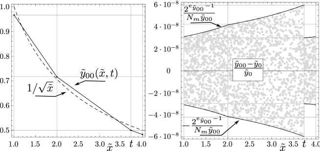
Figure 2: Left: function $1/\sqrt{\tilde{x}}\,$ and its zeroth approximation $\tilde{y}_{00}(\tilde{x},t)$ given by (3.17). Right: relative error of the zeroth approximation $\tilde{y}_{00}(\tilde{x},t)$ for $2000$ random values of $\tilde{x}$.

In order to improve the accuracy, the zeroth approximation ($\tilde{y}_{00}$) is corrected twice using the Newton-Raphson method (lines 6 and 7 in the InvSqrt code):

$$\tilde{y}_{01} =\tilde{y}_{00}-f(\tilde{y}_{00})/f^{\prime}(\tilde{y}_{00}),$$

$$\tilde{y}_{02} =\tilde{y}_{01}-f(\tilde{y}_{01})/f^{\prime}(\tilde{y}_{01}),$$

where $f(y)=y^{-2}-x$. Therefore:

$$\tilde{y}_{01}(\tilde{x},t) =2^{-1}\tilde{y}_{00}(\tilde{x},t)(3-\tilde{y}_{00}^{2}(\tilde{x},t)\,\tilde{x}),$$ (3.19)

$$\tilde{y}_{02}(\tilde{x},t) =2^{-1}\tilde{y}_{01}(\tilde{x},t)(3-\tilde{y}_{01}^{2}(\tilde{x},t)\,\tilde{x}).$$ (3.20)

In this section we gave a theoretical explanation of the InvSqrt code. In the original form of the code the magic constant $R$ was guessed. Our interpretation gives us a natural possibility to treat $R$ as a free parameter. In next section we will find its optimal values, minimizing errors.

4 Minimization of the relative error

Approximations of the inverse square root presented in the previous section depend on the parameter $t$ directly related to the magic constant. The value of this parameter can be estimated by analysing the relative error of $\tilde{y}_{0k}(\tilde{x},t)$ with respect to $\sqrt{\tilde{x}}$:

$$\tilde{\delta}_{k}(\tilde{x},t)=\sqrt{\tilde{x}}\tilde{y}_{0k}(\tilde{x},t)-1,\quad\text{where: $k\in\{0,1,2\}$}.$$ (4.1)

As the best estimation we consider $t=t_{k}^{(r)}$ minimizing the relative error $\tilde{\delta}_{k}(\tilde{x},t)$:

$$\forall_{t\neq t_{k}^{(r)}}\max_{\tilde{x}\in\tilde{A}}|\tilde{\delta}_{k}(\tilde{x},t_{k}^{(r)})|<\max_{\tilde{x}\in\tilde{A}}|\tilde{\delta}_{k}(\tilde{x},t)|\quad\text{where: $\tilde{A}=\tilde{A}^{I}\cup\tilde{A}^{II}\cup\tilde{A}^{III}$}.$$ (4.2)

4.1 Zeroth approximation

In order to determine $t_{0}^{(r)}$ we have to find extrema of $\tilde{\delta}_{0}(\tilde{x},t)$ with respect to $\tilde{x}$, to identify maxima, and to compare them with boundary values $\tilde{\delta}_{0}(1,t)=\tilde{\delta}^{I}_{0}(1,t)$, $\tilde{\delta}_{0}(2,t)=\tilde{\delta}^{I}_{0}(2,t)=\tilde{\delta}^{II}_{0}(2,t)$, $\tilde{\delta}_{0}(t,t)=\tilde{\delta}^{II}_{0}(t,t)=\tilde{\delta}^{III}_{0}(t,t)$, $\tilde{\delta}_{0}(4,t)=\tilde{\delta}^{III}_{0}(4,t)$ at the ends of the considered intervals $\tilde{A}^{I}$, $\tilde{A}^{II}$, $\tilde{A}^{III}$. Equating to zero derivatives of $\tilde{\delta}_{0}^{I}(\tilde{x},t)$, $\tilde{\delta}_{0}^{II}(\tilde{x},t)$, $\tilde{\delta}_{0}^{III}(\tilde{x},t)$:

$$0 =\partial_{\tilde{x}}\tilde{\delta}_{0}^{I}(\tilde{x},t)=2^{-3}x^{-1/2}(3-3x+2^{-1}t),$$

$$0 =\partial_{\tilde{x}}\tilde{\delta}_{0}^{II}(\tilde{x},t)=2^{-2}x^{-1/2}(1-3\cdot 2^{-2}x+2^{-2}t),$$

$$0 =\partial_{\tilde{x}}\tilde{\delta}_{0}^{III}(\tilde{x},t)=2^{-2}x^{-1/2}(1-3\cdot 2^{-3}x+2^{-3}t),$$ (4.3)

we find local extrema:

$$\tilde{x}_{0}^{I}=(6+t)/6,\quad\tilde{x}_{0}^{II}=(4+t)/3,\quad\tilde{x}_{0}^{III}=(8+t)/3.,$$ (4.4)

We easily verify that $\tilde{\delta}_{0}^{I}(\tilde{x},t)$, $\tilde{\delta}_{0}^{II}(\tilde{x},t)$, $\tilde{\delta}_{0}^{III}(\tilde{x},t)$ are concave functions:

$$\partial^{2}_{\tilde{x}}\tilde{\delta}_{0}^{K}(\tilde{x},t)<0,\quad\text{for: $K\in\{I,II,III\}$}$$

which means that we have local maxima at $\tilde{x}_{0}^{K}$ (where $K\in\{I,II,III\}$). One of them is negative:

$$\tilde{\delta}_{0m}^{III}(t)=\tilde{\delta}_{0}(\tilde{x}_{0}^{III},t)=-2^{-1}+2^{-3}t<0\quad\text{for $t\in(2,4)$}.$$

The other maxima, given by

$$\tilde{\delta}_{0m}^{I}(t) =\tilde{\delta}_{0}(x_{0}^{I},t)=-1+2^{-1}(1+t/6)^{3/2},$$

$$\tilde{\delta}_{0m}^{II}(t) =\tilde{\delta}_{0}(x_{0}^{II},t)=-1+2\cdot 3^{-3/2}(1+t/4)^{3/2},$$ (4.5)

are increasing functions of $t$, satisfying

$$\tilde{\delta}_{0m}^{II}(t) <\tilde{\delta}_{0m}^{I}(t)\quad\wedge\quad\tilde{\delta}_{0m}^{I}(t)\leq 0, \text{for $t\in(2,3\cdot 2^{5/3}-6\rangle$},$$ (4.6)

$$\tilde{\delta}_{0m}^{II}(t) <\tilde{\delta}_{0m}^{I}(t)\quad\wedge\quad\tilde{\delta}_{0m}^{I}(t)>0, \text{for $t\in(3\cdot 2^{5/3}-6,2^{5/3}+2^{4/3}-2)$},$$ (4.7)

$$\tilde{\delta}_{0m}^{II}(t) \geq\tilde{\delta}_{0m}^{I}(t)\quad\wedge\quad\tilde{\delta}_{0m}^{I}(t)>0, \text{for $t\in\langle 2^{5/3}+2^{4/3}-2,4)$}.$$ (4.8)

Because functions $\tilde{\delta}_{0}^{I}(\tilde{x},t)$, $\tilde{\delta}_{0}^{II}(\tilde{x},t)$, $\tilde{\delta}_{0}^{III}(\tilde{x},t)$ are concave, their minimal values with respect to $\tilde{x}$ are assumed at boundaries of the intervals $\tilde{A}^{I}$, $\tilde{A}^{II}$, $\tilde{A}^{III}$. It turns out that the global minimum is described by the following function:

$$\tilde{\delta}_{0}^{II}(t,t)=\tilde{\delta}_{0}^{III}(t,t)=-1+2^{-1}\sqrt{t},$$ (4.9)

which is increasing and negative for $t\in(2,4)$. Therefore, taking into account (4.6), (4.7) and (4.8), the condition (4.2) reduces to

$$\tilde{\delta}_{0m}^{I}(t_{0}^{(r)}) =|\tilde{\delta}_{0}^{II}(t_{0}^{(r)},t_{0}^{(r)})| \text{for \ \ $t_{0}^{(r)}\in(2,-2+2^{4/3}+2^{5/3})$},$$ (4.10)

$$\tilde{\delta}_{0m}^{II}(t_{0}^{(r)}) =|\tilde{\delta}_{0}^{II}(t_{0}^{(r)},t_{0}^{(r)})| \text{for \ \ $t_{0}^{(r)}\in\langle-2+2^{4/3}+2^{5/3},4)$}.$$ (4.11)

The right answer results from equation (4.11):

$$t_{0}^{(r)}\simeq 3.7309796.$$ (4.12)

Thus we obtain an estimation minimizing maximal relative error of zeroth approximation:

$$\delta_{0\max}=\max_{\tilde{x}\in\tilde{A}}|\delta_{0}(\tilde{x},t_{0}^{(r)})|=|\delta_{0}(t_{0}^{(r)},t_{0}^{(r)})|\simeq 0.03421281,$$ (4.13)

and the magic constant $R_{0}^{(r)}$:

$$R_{0}^{(r)} =N_{m}(e_{R}+B)+\lfloor 2^{-2}N_{m}(t_{0}^{(r)}-2)-2^{-1}\rceil=$$

$$=1597465647=0x5F37642F\,.$$ (4.14)

The resulting relative error is presented at Fig.3.

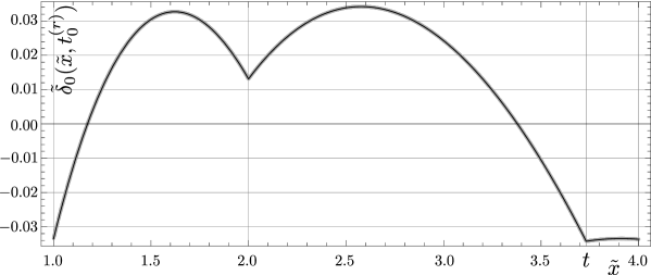
Figure 3: Relative error for zeroth approximation of the inverse square root. Grey points were generated by the function InvSqrt without two lines ($6$ and $7$) of code and with $R=R_{0}^{(r)}$, for $4000$ random values $x\in\langle 2^{-126},2^{128})$.

4.2 Newton-Raphson corrections

The relative error can be reduced by Newton-Raphson corrections (3.19) and (3.20). Substituting $\tilde{y}_{0k}(\tilde{x},t)=(1+\tilde{\delta}_{k}(\tilde{x},t))/\sqrt{\tilde{x}}$   we rewrite them as

$$\tilde{\delta}_{k}(\tilde{x},t)=-\frac{1}{2}\tilde{\delta}_{k-1}^{2}(3+\tilde{\delta}_{k-1}(\tilde{x},t)),\quad\text{where: $k\in\{1,2\}$}.$$ (4.15)

The quadratic dependence on $\tilde{\delta}_{k-1}$ implies a fast convergence of the Newton-Raphson iterations. Note that obtained functions $\tilde{\delta}_{k}$ are non-positive. Their derivatives with respect to $\tilde{x}$ can be easily calculated

$$\partial_{\tilde{x}}\tilde{\delta}_{k}(\tilde{x},t) =-\frac{3}{2}\tilde{\delta}_{k-1}(\tilde{x},t)(2+\tilde{\delta}_{k-1}(\tilde{x},t))\partial_{\tilde{x}}\tilde{\delta}_{k-1}(\tilde{x},t)$$

$$\partial^{2}_{\tilde{x}}\tilde{\delta}_{k}(\tilde{x},t) =-\frac{3}{2}\tilde{\delta}_{k-1}(\tilde{x},t)(2+\tilde{\delta}_{k-1}(\tilde{x},t))\partial^{2}_{\tilde{x}}\tilde{\delta}_{k-1}(\tilde{x},t)+$$

$$-3(\tilde{\delta}_{k-1}(\tilde{x},t)+1)[\partial_{\tilde{x}}\tilde{\delta}_{k-1}(\tilde{x},t)]^{2}$$

One can easily see that that extremes of $\tilde{\delta}_{k}$ can be determined by studying extremes and zeros of $\tilde{\delta}_{k-1}$.

• Local maxima of $\tilde{\delta}_{k}(\tilde{x},t)$ correspond to negative local minima of $\tilde{\delta}_{k-1}(\tilde{x},t)$ or for zeros of $\tilde{\delta}_{k-1}(\tilde{x},t)$. However, a local maximum of a non-positive function can not be a candidate for a global maximum of its modulus (compare (4.2)).

• Local minima of $\tilde{\delta}_{k}(\tilde{x},t)$ correspond to positive maxima and negative minima of $\tilde{\delta}_{k-1}(\tilde{x},t)$, which means that they are given by $\tilde{\delta}_{0m}^{I}(t)$, $\tilde{\delta}_{0m}^{II}(t)$, see (4.5).

Then, we compute

$$\frac{\partial\tilde{\delta}_{k}(\tilde{x},t)}{\partial\tilde{\delta}_{k-1}(\tilde{x},t)}=-\frac{3}{2}\tilde{\delta}_{k-1}(\tilde{x},t)(2+\tilde{\delta}_{k-1}(\tilde{x},t)),$$ (4.16)

which implies that $\tilde{\delta}_{k}(\tilde{x},t)$ is an increasing function of $\tilde{\delta}_{k-1}(\tilde{x},t)$ for $\tilde{\delta}_{k-1}(\tilde{x},t)<0$ and a decreasing function of $\tilde{\delta}_{k-1}(\tilde{x},t)$ for $\tilde{\delta}_{k-1}(\tilde{x},t)>0$. It means that there only two candidates for the minimum of $\tilde{\delta}_{1}(\tilde{x},t)$: one corresponding to the minimal negative value of $\tilde{\delta}_{k-1}(\tilde{x},t)$ and one corresponding to the maximal positive value of $\tilde{\delta}_{k-1}(\tilde{x},t)$. The smallest value of $\tilde{\delta}_{k}(\tilde{x},t)$ evaluated at boundaries of regions $\tilde{A}^{I}$, $\tilde{A}^{II}$ and $\tilde{A}^{III}$ still is assumed at $\tilde{x}=t$.

In the case $k=1$ (the first Newton-Raphston correction) we have negative minima ($\tilde{\delta}_{1m}^{I}(t)$ and $\tilde{\delta}_{1m}^{II}(t)$) corresponding to positive maxima of $\tilde{\delta}_{0}(\tilde{x},t)$. The minima are decreasing functions of $t$ and satisfy conditions

$$|\tilde{\delta}_{1m}^{II}(t)| <|\tilde{\delta}_{1m}^{I}(t)|\quad\text{for $t\in(2,-2+2^{4/3}+2^{5/3})$},$$ (4.17)

$$|\tilde{\delta}_{1m}^{II}(t)| \geq|\tilde{\delta}_{1m}^{I}(t)|\quad\text{for $t\in\langle-2+2^{4/3}+2^{5/3},4)$}.$$ (4.18)

In the case $k=2$ we get minima at the same locations as for $k=1$ and with the same monotonicity with respect to $t$. All this leads to the conclusion that the condition (4.2) for the first and second correction will be satisfied for the same value $t=t_{1}^{(r)}=t_{2}^{(r)}$ (smaller than $t_{0}^{(r)}$):

$$t_{1}^{(r)}=t_{2}^{(r)}\simeq 3.7298003\,,$$ (4.19)

where $t_{1}^{(r)}$ is a solution to the equation

$$\tilde{\delta}_{1}(t_{1}^{(r)},t_{1}^{(r)})=\tilde{\delta}_{1}(\underbrace{4/3+t_{1}^{(r)}/3}_{\tilde{x}_{0}^{II}},t_{1}^{(r)}).$$ (4.20)

Thus we obtained a new estimation of the magic constant:

$$R_{1}^{(r)}=R_{2}^{(r)} =N_{m}(e_{R}+B)+\lfloor 2^{-2}N_{m}(t_{1}^{(r)}-2)-2^{-1}\rceil=$$

$$=1597463174=0x5F375A86\,$$ (4.21)

with corresponding maximal relative errors:

$$\begin{array}[]{l}\tilde{\delta}_{1\max}=|\tilde{\delta}_{1}(t_{1}^{(r)},t_{1}^{(r)})|\simeq 1.75118\cdot 10^{-3}\,,\\[7.74997pt] \tilde{\delta}_{2\max}=|\tilde{\delta}_{2}(t_{1}^{(r)},t_{1}^{(r)})|\simeq 4.60\cdot 10^{-6}\,.\end{array}$$ (4.22)

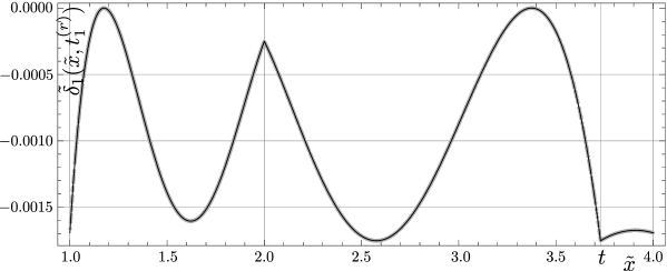
Figure 4: Relative error of the first Newton-Raphson correction of the inverse square root approximation. Grey points were generated by the fuction InvSqrt without line 7 of the code and with $R=R_{1}^{(r)}$, for $4000$ random values $x\in\langle 2^{-126},2^{128})$.

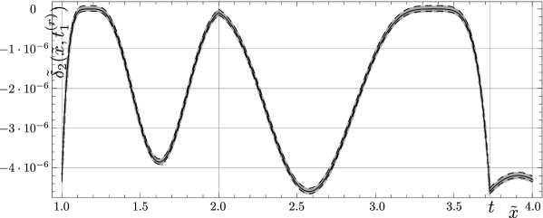
Figure 5: Relative error of the second Newton-Raphson correction of the inverse square root approximation. Grey points were generated by the function InvSqrt z $R=R_{1}^{(r)}=R_{2}^{(r)}$, for $4000$ random values $x\in\langle 2^{-126},2^{128})$. The visible blur is a consequence of round-off errors.

5 Minimization of the absolute error

Similarly as in the previous section we will derive optimal values of the magic constant minimizing the absolute error of approximations $\tilde{y}_{00}(\tilde{x},t)$, $\tilde{y}_{01}(\tilde{x},t)$ and $\tilde{y}_{02}(\tilde{x},t)$, i.e., by minimizing

$$\tilde{\Delta}_{k}(\tilde{x},t)=\tilde{y}_{0k}(\tilde{x},t)-1/\sqrt{\tilde{x}},\qquad\quad k\in\{0,1,2\}.$$ (5.1)

In other words, we will find $t_{0}^{(a)}$, $t_{1}^{(a)}$ and $t_{2}^{(a)}$ such that

$$\forall_{t\neq t_{k}^{(a)}}\max_{\tilde{x}\in\tilde{A}}|\tilde{\Delta}_{k}(\tilde{x},t_{k}^{(a)})|<\max_{\tilde{x}\in\tilde{A}}|\tilde{\Delta}_{k}(\tilde{x},t)|$$ (5.2)

for $k=0,1,2$, where  $\tilde{A}=\tilde{A}^{I}\cup\tilde{A}^{II}\cup\tilde{A}^{III}$.

5.1 Zeroth approximation

In order to find $t_{0}^{(a)}$ minimizing the absolute error of $\tilde{y}_{00}(\tilde{x},t)$, we will compute and study extremes of $\tilde{\Delta}_{0}(\tilde{x},t)$ inside intervals $\tilde{A}^{I}$, $\tilde{A}^{II}$ and $\tilde{A}^{III}$, and compare them with values of $\tilde{\Delta}_{0}(\tilde{x},t)$ at the ends of the intervals. First, we compute the boundary values:

$$\begin{array}[]{l}\displaystyle\tilde{\Delta}_{0}(1,t)=\frac{t}{8}-\frac{1}{2},\\[7.74997pt] \displaystyle\tilde{\Delta}_{0}(2,t)=\frac{t}{8}-\frac{2\sqrt{2}-1}{4},\\[7.74997pt] \displaystyle\tilde{\Delta}_{0}(t,t)=\frac{1}{2}-\frac{1}{\sqrt{t}},\\[7.74997pt] \displaystyle\tilde{\Delta}_{0}(4,t)=\frac{t}{16}-\frac{1}{4}.\\[7.74997pt] \end{array}$$ (5.3)

All of them are negative (for $t<4$). Derivatives of error functions ($\tilde{\Delta}_{0}^{I}(\tilde{x},t)$, $\tilde{\Delta}_{0}^{II}(\tilde{x},t)$ and $\tilde{\Delta}_{0}^{III}(\tilde{x},t)$) are given by:

$$\begin{array}[]{l}\displaystyle\partial_{\tilde{x}}\tilde{\Delta}_{0}^{I}(\tilde{x},t)=2^{-1}\tilde{x}^{-3/2}-2^{-2},\\[3.87498pt] \displaystyle\partial_{\tilde{x}}\tilde{\Delta}_{0}^{II}(\tilde{x},t)=2^{-1}\tilde{x}^{-3/2}-2^{-3},\\[3.87498pt] \displaystyle\partial_{\tilde{x}}\tilde{\Delta}_{0}^{III}(\tilde{x},t)=2^{-1}\tilde{x}^{-3/2}-2^{-4}.\end{array}$$ (5.4)

Therefore local extrema are located at

$$\tilde{x}_{0a}^{I}=2^{2/3},\qquad\tilde{x}_{0a}^{II}=2^{4/3},\qquad\tilde{x}_{0a}^{III}=4$$ (5.5)

(the locations do not depend on $t$). The second derivative is negative:

$$\partial^{2}_{\tilde{x}}\tilde{\Delta}_{0}^{K}(\tilde{x},t)=-3\cdot 2^{-2}x^{-5/2}<0$$

for   $K\in\{I,II,III\}$. Therefore all these extremes are local maxima, given by

$$\begin{array}[]{l}\displaystyle\tilde{\Delta}_{0}(\tilde{x}_{0a}^{I},t)=\tilde{y}^{I}_{0}(\tilde{x}_{0a}^{I},t)-(\tilde{x}_{0a}^{I})^{-1/2}=\frac{3}{4}-\frac{3}{2\sqrt[3]{2}}+\frac{1}{8}t,\\[7.74997pt] \displaystyle\tilde{\Delta}_{0}(\tilde{x}_{0a}^{II},t)=\tilde{y}^{II}_{0}(\tilde{x}_{0a}^{II},t)-(\tilde{x}_{0a}^{II})^{-1/2}=\frac{1}{2}-\frac{3\sqrt[3]{2}}{4}+\frac{1}{8}t,\\[7.74997pt] \displaystyle\tilde{\Delta}_{0}(\tilde{x}_{0a}^{III},t)=\tilde{y}^{III}_{0}(\tilde{x}_{0a}^{III},t)-(\tilde{x}_{0a}^{III})^{-1/2}=\frac{1}{16}t-\frac{1}{4}.\end{array}$$ (5.6)

We see that $\tilde{\Delta}_{0}(\tilde{x}_{0a}^{III},t)<0$ for $t<4$ (and negative maxima obviously are not important). Direct computation shows that for $t\leqslant 4$ the first value of (5.6) is the greatest, i.e.,

$$\max_{\tilde{x}\in\tilde{A}}\tilde{\Delta}_{0}(\tilde{x},t)=\tilde{\Delta}_{0}(\tilde{x}_{0a}^{I},t)$$ (5.7)

Evaluating $\tilde{\Delta}_{0}(\tilde{x},t)$ at the ends of the intervals $\tilde{A}^{I}$, $\tilde{A}^{II}$ and $\tilde{A}^{III}$, we find the global minimum:

$$\min_{\tilde{x}\in\tilde{A}}\tilde{\Delta}_{0}(\tilde{x},t)=\tilde{\Delta}^{I}_{0}(1,t)=-\frac{1}{2}+\frac{t}{8}<0,$$ (5.8)

which enables us to formulate the condition (5.2) in the following form:

$$\max_{\tilde{x}\in\tilde{A}}\tilde{\Delta}_{0}(\tilde{x},t)=|\min_{\tilde{x}\in\tilde{A}}\tilde{\Delta}_{0}(\tilde{x},t)|\quad\Leftrightarrow\quad\frac{3}{4}-\frac{3}{2\sqrt[3]{2}}+\frac{1}{8}t=\frac{1}{2}-\frac{t}{8}.$$ (5.9)

Solving this equation we get:

$$t_{0}^{(a)}=-1+3\cdot 2^{2/3}\simeq 3.7622,$$ (5.10)

which corresponds to a magic constant $R_{0}^{(a)}$ given by

$$R_{0}^{(a)}=N_{m}(e_{R}+B)+\lfloor 2^{-2}N_{m}(t_{0}^{(a)}-2)-2^{-1}\rceil=1597531127=0x5F3863F7.$$ (5.11)

The resulting maximal error of the zeroth approxmation reads

$$\Delta_{0\max}=\max_{\tilde{x}\in\tilde{A}}|\Delta_{k}(\tilde{x},t_{k}^{(a)})|=\frac{5}{8}-\frac{3}{4\sqrt[3]{2}}\simeq 0.0297246.$$ (5.12)

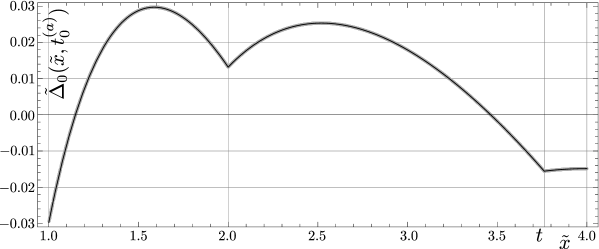
Figure 6: Absolute error of zeroth approximation of the inverse square root. Grey points were generated by the function InvSqrt without two lines ($6$ and $7$) of the code and with $R=R_{0}^{(a)}$, for $4000$ random values $x\in\langle 1,4)$.

5.2 Newton-Raphson corrections

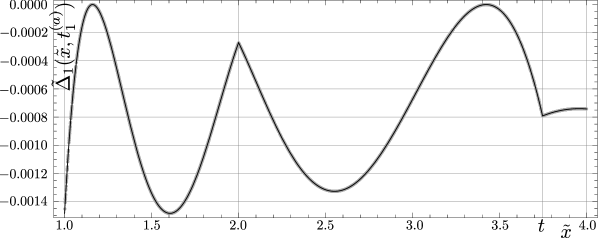
Figure 7: Absolute error of the first Newton-Raphson correction of the inverse square root approximation. Grey points were generated by the function InvSqrt without the line $7$ of the InvSqrt code and with $R=R_{1}^{(a)}$, for $4000$ random values $\tilde{x}\in\langle 1,4)$.

The absolute errror after Newton-Raphson corrections is a non-positive function, similarly as the relative error. This function reaches its maximal value equal to zero in intervals $\tilde{A}^{I}$ and $\tilde{A}^{II}$ (which corresponds to zeros of $\tilde{\Delta}_{0}^{I}$ i $\tilde{\Delta}_{0}^{II}$) and has a negative maximum in the interval $\tilde{A}^{III}$. The other extremes (minima) are decreasing functions of the parameter $t$. They are located at $x$ defined by the following equations:

$$0= -\frac{75}{128}-\frac{27t}{256}-\frac{9t^{2}}{512}-\frac{t^{3}}{1024}+\frac{1}{2x^{3/2}}+\frac{27x}{64}+\frac{9tx}{64}+\frac{3t^{2}x}{256}-\frac{27x^{2}}{128}+$$

$$-\frac{9tx^{2}}{256}+\frac{x^{3}}{32},\;\;\qquad\qquad\qquad\qquad\text{for $x\in\tilde{A}^{I}$},$$ (5.13)

$$0= -\frac{1}{4}-\frac{3t}{64}-\frac{3t^{2}}{256}-\frac{t^{3}}{1024}+\frac{1}{2x^{3/2}}+\frac{3x}{32}+\frac{3tx}{64}+\frac{3t^{2}x}{512}-\frac{9x^{2}}{256}+$$

$$-\frac{9tx^{2}}{1024}+\frac{x^{3}}{256},\qquad\qquad\qquad\qquad\text{for $x\in\tilde{A}^{II}$}.$$ (5.14)

The condition (5.2) reduces to the equality of the local minimum (located in $\tilde{A}^{I}$) and $\tilde{\Delta}_{1}(1,t)$ (this is an increasing function of $t$). The equality is obtained for $t=t_{1}^{(a)}$, where

$$t_{1}^{(a)}\simeq 3.74699138,$$ (5.15)

The corresponding maximal error and a magic constant are given by

$$\Delta_{1\max}\simeq 0.001484497,$$ (5.16)

$$R_{1}^{(a)}=1597499226=0x5F37E75A\,.$$ (5.17)

In the case of the second Newton-Raphson correction the minimization of errors is obtained similarly, by equating the local minimum $\tilde{\Delta}_{2}^{I}(\tilde{x},t)$ with $\tilde{\Delta}_{2}^{I}(1,t)$. Hence we get another value a magic constant:

$$R_{2}^{(a)}=1597484501=0x5F37ADD5,$$ (5.18)

corresponding to

$$t_{2}^{(a)}\simeq 3.73996986,\quad\Delta_{2\max}\simeq 3.684\cdot 10^{-6}.$$ (5.19)

Figure 8: Absolute error of the second Newton-Raphson correction of the inverse square root approximation. Grey points were generated by the function InvSqrt of the InvSqrt code and with $R=R_{2}^{(a)}$, for $4000$ random values $\tilde{x}\in\langle 1,4)$.

6 Conclusions

In this paper we have presented a theoretical interpretation of the InvSqrt code, giving a precise meaning to two values of the magic constant exisiting in the literature and adding two more values of the magic constant. Using this magic constant we have conducted error analysis for Newton-Raphson Method and proved that error bounds for single precision computation are acceptable. The magic constant can be easily incorporated in existing floating point multiplier or floating point multiply-add fused and one need to replace LUT with the magic constant.

References

- [1] M. Sadeghian and J. Stine: “Optimized Low-Power Elementary Function Approximation for Chybyshev series Approximation“, 46th Asilomar Conf. on Signal Systems and Computers, 2012.
- [2] K. Diefendorff, P. K. Dubey, R. Hochprung and H. Scales: “Altivec Extension to PowerPC Accelerates Media Processing“, IEEE Micro, pp. 85-95, Mar./Apr. 2000.
- [3] D. Harris: “A Powering Unit for an OpenGL Lighting Engine“, Proc. 35th Asilomar Conf. Singals, Systems, and Computers, pp. 1641-1645, 2001.
- [4] D. M. Russinoff: A Mechanically Checked Proof of Correctness of the AMD K5 Floating Point Square Root Microcode, Formal Methods in System Design, Vol.14, Issue 1, pp. 75-125,Jan 1999.
- [5] J-M Muller, N. Brisebarre, F. Dinechin, C-P. Jeannerod, V. Lefèvre, G. Melquiond, N. Revol, D.Stehlé and S. Torres: Software Implementation of Floating-Point Arithmetic, Handbook of Floating-Point Arithmetic, pp. 321-372, Oct 2009.
- [6] D. E. Metafas and C. E. Goutis: A floating-point advanced cordic processor,Journal of VLSI signal processing systems for signal, image and video technology, Vol.10, Issue 1, pp 53-65, Jan 1995.
- [7] M.Cornea, C. Anderson and C. Tsen: Software Implementation of the IEEE 754R Decimal Floating-Point Arithmetic,Software and Data Technologies, Vol. 10 of the series Communications in Computer and Information Science pp. 97-109.
- [8] J-M Muller, N. Brisebarre, F. Dinechin, C-P. Jeannerod, V. Lefèvre, G. Melquiond, N. Revol, D.Stehlé and S. Torres: Hardware Implementation of Floating-Point Arithmetic, Handbook of Floating-Point Arithmetic, pp. 269-320, Oct 2009.
- [9] D.H.Eberly: GPGPU Programming for Games and Science, CRC Press 2015.
- [10] N.Ide, M.Hirano, Y.Endo, S.Yoshioka, H.Murakami, A.Kunimatsu, T.Sato, T.Kamei, T.Okada, and M.Suzuki: “2. 44-GFLOPS 300-MHz Floating-Point Vector-Processing Unit for High-Performance 3D Graphics Computing“, IEEE J. Solid-State Circuits, vol. 35, no. 7, pp. 1025-1033, July 2000.
- [11] S. Oberman,G. Favor and F. Weber :(AMD 3DNow! technology: architecture and implementations. IEEE Micro, Vol.9, No.2, pp. 37-48, Mar/Apr. 1999.
- [12] W. Liu and A. Nammarelli: “Power Efficient Division and Square root Unit“, IEEE Trans. Comp, vol. 61, No.8, pp. 1059-1070, Aug 2012.
- [13] T .J. Kwon and J. Draper: “Floating-point Division and Square root Implementation using a Taylor-Series Expan- sion Algorithm with Reduced Look-Up Table“, 51st Midwest Symposium on Circuits and Systems, 2008.
- [14] L.. Xuan and D. J. An: “A low latency High-throughput Elementary Function Generator based on Enhanced double rotation CORDIC“, Symposium on Computer Applications and Communications, 2014.
- [15] M. X. Nguyen and A. Dinh-Duc: “Hardware-Based Algorithm for Sine and Cosine Computations using Fixed Point Processor, 11th International Conf. on Electrical Engineering/Electronics Computer, Telecommunca- tions and Information Technology, 2014.
- [16] B. Paharami: Computer Arithmetic Algorithms and Hardware Designs, Oct 2010.
- [17] id software, quake3-1.32b/code/game/q_math.c , Quake III Arena, 1999.
- [18] C. Lomont, ”Fast inverse square root,” Purdue University, Tech. Rep., 2003. Available online: http://www.matrix67.com/data/InvSqrt.pdf, http://www.lomont.org/Math/Papers/2003/InvSqrt.pdf.
- [19] S.Zafar, R.Adapa: Hardware architecture design and mapping of ”Fast Inverse Square Root’s algorithm”, Advances in Electrical Engineering (ICAEE), 2014 International Conference on. - IEEE, 2014. - pp. 1-4.
- [20] J.Blinn, Floating-point tricks, IEEE Computer Graphics and Applications 17 (4) (1997) 80-84.
- [21] Q.Avril, V. Gouranton and B. Arnaldi: Fast Collision Culling in Large-Scale Environments Using GPU Mapping Function, ACM Eurographics Parallel Graphics and Visualization, Cagliari, Italy (2012).
- [22] E.Ardizzone, R.Gallea, O.Gambino, R.Pirrone: Effective and Efficient Interpolation for Mutual Information based Multimodality Elastic Image Registration, 2003.
- [23] J.L.V.M. Stanislaus, T.Mohsenin: High Performance Compressive Sensing Reconstruction Hardware with QRD Process, IEEE International Symposium on Circuits and Systems (ISCAS ’ 12), May 2012.
- [24] M.Robertson: A Brief History of InvSqrt, Bachelor Thesis, Univ. of New Brunswick 2012.
- [25] D.Eberly: Fast inverse square root, Geometric Tools, LLC(2010), http://geometrictools.com/Documentation/FastInverseSqrt.pdf.
- [26] C.McEniry: The Mathematics Behind the Fast Inverse Square Root Function Code, Tech. rep. 2007.
- [27] B.Self: Efficiently Computing the Inverse Square Root Using Integer Operations. May 31, 2012.