Analytical forms of chaotic spiral arms

Abstract

We develop an analytical theory of chaotic spiral arms in galaxies. This is based on the Moser theory of invariant manifolds around unstable periodic orbits. We apply this theory to the chaotic spiral arms, that start from the neighborhood of the Lagrangian points $L_{1}$ and $L_{2}$ at the end of the bar in a barred-spiral galaxy. The series representing the invariant manifolds starting at the Lagrangian points $L_{1}$, $L_{2}$, or unstable periodic orbits around $L_{1}$ and $L_{2}$, yield spiral patterns in the configuration space. These series converge in a domain around every Lagrangian point, called “Moser domain” and represent the orbits that constitute the chaotic spiral arms. In fact, these orbits are not only along the invariant manifolds, but also in a domain surrounding the invariant manifolds. We show further that orbits starting outside the Moser domain but close to it converge to the boundary of the Moser domain, which acts as an attractor. These orbits stay for a long time close to the spiral arms before escaping to infinity.

1 Introduction

An important development in the theory of nonlinear dynamical systems was provided by Moser (1956, 1958) who proved the convergence of the normal form series describing the Hamiltonian dynamics near an unstable equilibrium point, or an unstable periodic orbit. This convergence allows to study chaotic orbits by analytical means, i.e. using series. This is in contrast with what happens in the case of the usual Birkhoff normal form series around stable invariant points, or stable periodic orbits; it is well known that these series do not converge, but they are only asymptotic (see Contopoulos (2002) for a review).

In the present paper we present a connection between Moser’s theorem and the so-called manifold theory of chaotic spiral arms in rotating barred galaxies. The manifold theory was proposed in 2006 (Voglis et al., 2006b; Romero-Gomez et al., 2006) and was explored in detail in a number of subsequent papers (Romero-Gomez et al., 2007; Tsoutsis et al., 2008, 2009; Athanassoula et al., 2009a, b; Harsoula et al., 2011; Athanassoula, 2012). The theory predicts a number of morphological correlations between the spiral arms and the bar strength and/or the pattern speed (see Pérez-Villegas et al. (2015) for comparison of these features with observations as well as Dobbs & Baba (2014) for a review).

The basic element of the manifold theory stems from the form of the unstable invariant manifolds of the family of short-period Lyapunov orbits around the unstable Lagrangian equilibria $L_{1}$ or $L_{2}$ at the end of the bar (see section 2). These manifolds, when projected in the configuration space, take the form of trailing spiral arms. In the manifold picture, the spiral arms in barred galaxies are density waves, but, contrary to the case of normal galaxies, they are composed of chaotic orbits. The backbone of the spiral arms can be due to the pattern formed by the orbits either all along the unstable manifolds (Romero-Gomez et al., 2006), or only at the apsidal positions along the manifolds (Voglis et al., 2006b); see Efthymiopoulos (2010), for a discussion of the differences between these two models). Furthermore, the chaotic orbits of the manifold theory can exhibit two distinct behaviors, i.e., i) they can lead to escapes without recurrences, or ii) they can have a (possibly quite large) number of recurrences inside and outside the corotation region. The orbits which exhibit recurrences belong to a more general chaotic population known as the ‘hot population’ (Sparke & Sellwood, 1987; Kaufmann & Contopoulos, 1996). Finally, not only the orbits connected with $L_{1}$ or $L_{2}$, but also those connected to other unstable periodic orbits in the corotation region may exhibit similar features and support the chaotic spiral arms (Patsis, 2006; Tsoutsis et al., 2008).

Although from a geometrical point of view the invariant manifolds define spiral patterns, it is a basic fact that their measure is zero in the entire set of all possible initial conditions in the chaotic phase space at the corotation region. On the other hand, the observed spiral arms can only correspond to a non-zero phase space density of stars. Thus, the question is, how can we build domains of chaotic orbits, of non-zero measure, around the invariant manifolds. Our answer in this paper is based on Moser’s theorem. Namely, we will argue below that these domains correspond to the domains of convergence of the Moser normal form around the unstable manifolds.

So far, Moser’s theorem was applied in very simple dynamical systems like mappings (Franceschini & Russo, 1981; da Silva Ritter et al., 1987). In simple cases it was shown that the convergence domain extends to infinity along the invariant manifolds. Further work on the Moser series allowed us to find the limits of convergence also away from the invariant manifolds (Efthymiopoulos et al., 2014; Harsoula et al., 2015). Furthermore, in these simple systems it was possible to find the Moser domains of convergence of several unstable periodic orbits. By their overlapping we could find analytically the heteroclinic points between the various resonances (Contopoulos & Harsoula, 2015). A key result of these studies regards the asymptotic (in time) behavior of the chaotic orbits with initial conditions inside or outside a Moser domain of convergence. Namely, we found that orbits starting outside (but close to) the convergence domain approach arbitrarily close to the outer limits of this domain asymptotically in time (although they can never enter inside it). On the other hand, the chaotic orbits with initial conditions inside the Moser domain can never exit this domain. In conclusion, the Moser domain of convergence provides a bounded set of chaotic orbits on non-zero measure which remain always close to the invariant manifolds, while the boundary of this domain acts as an attractor for all the chaotic initial conditions exterior to the domain (and close enough to the boundary, see section 3).

In the present paper, we apply the theory of Moser for orbits starting close to the Lagrangian points $L_{1}$ and $L_{2}$. In particular, we compute the Moser domain of convergence for normal form series built around the equilibria $L_{1}$ and $L_{2}$ in three different models of barred galaxies emerging from past numerical simulations (Voglis et al., 2006a). This allows to obtain analytically not only the form of the invariant manifolds, which define the spiral arms, but also the form of the Moser domain of convergence. Then, we show that this domain follows closely the spiral patterns, and provides a chaotic set of non-zero measure along the spiral patterns.

The paper is structured as follows: section 2 briefly presents a summary of the manifold theory and the models used in the present paper. Section 3 presents the normal form analytical computations, the computation of the Moser domain of convergence, based on high-order series expansions carried by a computer-algebraic program, and the results, which illustrate the connection between Moser domains and spiral patterns. In section 4 we provide a theoretical interpretation based on an approximative simplified mapping model. Finally, section 5 summarizes our basic conclusions.

2 Manifold theory and models

2.1 Manifold theory

The Hamiltonian of motion in the plane of a galaxy with a rotating bar for a test particle of mass $m=1$ is given by:

$$H={1\over 2}\left(p_{x}^{2}+p_{y}^{2}\right)-\Omega_{p}(xp_{y}-yp_{x})+\Phi(x,y)$$ (1)

where $x,y$ are the Cartesian positions in the rotating frame with pattern speed $\Omega_{p}$, $p_{x},p_{y}$ are the canonical momenta (velocities) in an instantaneous rest frame with axes ($x,y$), and $\Phi(x,y)$ is the gravitational potential of the galaxy in the rotating frame. For simplicity, we consider the potential as time-independent.

The unstable Lagrangian point $L_{1}$ (and similarly $L_{2}$) corresponds to a solution $(x,y,p_{x},p_{y})=(x_{L_{1}},y_{L_{1}},p_{xL_{1}},p_{yL_{1}})$ of the equilibrium equations $\partial{H}/\partial x$ $=$ $\partial{H}/\partial y$ $=$ $\partial{H}/\partial p_{x}$ $=$ $\partial{H}/\partial p_{y}$ $=0$. The equilibrium points $L_{1}$ and $L_{2}$ are located at the end of the bar, and they are simply unstable, i.e. the matrix of linearized equations around each of these points has two imaginary and two real eigenvalues $\lambda_{1,2}=\pm i\omega_{0}$, $\lambda_{3,4}=\pm\nu_{0}$, with $\omega_{0},\nu_{0}$ real. Then, we can introduce a symplectic change of variables $(x,y,p_{x},p_{y})$ $\rightarrow$ $(q,u,p,v)$, where ($q,p$) and ($u,v$) are conjugate pairs such that in the new variables the Hamiltonian can be expanded around $L_{1}$ (or $L_{2}$) as:

$$H=\omega_{0}\left({q^{2}+p^{2}\over 2}\right)+\nu_{0}uv+\sum_{s=3}^{\infty}P_{s}(q,p,u,v)$$ (2)

where the $P_{s}$ are polynomial functions of degree $s$. Let us neglect, to the lowest order limit, the effect of the terms $P_{s}$. Then, the motion in the $(q,p)$ plane reduces to the limit of a harmonic oscillation with frequency $\omega_{0}$, and the plane $(q,p)$ is called the linear center manifold of the equilibrium point $L_{1}$. On the other hand, the variable $u$ grows exponentially, $u=u_{0}e^{\nu_{0}t}$, while the variable $v$ decays exponentially as $v=v_{0}e^{-\nu_{0}t}$. Then, the $u$ axis defines the linear unstable manifold, and the $v$ axis the linear stable manifold of the equilibrium point $L_{1}$.

Back-transforming to the original cartesian variables, $(q,u,p,v)$ $\rightarrow$ $(x,y,p_{x},p_{y})$, the independent motions in the $(q,p)$ plane and in the $u$-axis, and $v$-axis lead to the following:

i) The oscillations in $(q,p)$ define retrograde epicyclic motions around $L_{1}$ with frequency $\omega_{0}$. In the full nonlinear problem, these are continued as a family of retrograde periodic orbits of period $2\pi/\omega$, around $L_{1}$, called the ‘short period family of orbits ’$PL_{1}$’ (Voglis et al., 2006b) or the horizontal ‘Lyapunov family of orbits’ (Romero-Gomez et al., 2006). In general we have $\omega\simeq\omega_{0}$, with the difference $\omega-\omega_{0}$ increasing with the size of the epicycle.

ii) The variable $u$ grows in the forward sense of time ($t\rightarrow\infty$). In Cartesian variables, this growth describes a recession of the guiding center of the epicycle away from $L_{1}$ in the trailing sense (see e.g. Fig.1 of Tsoutsis et al., 2009). Then, the combined guiding center and epicyclic motion forms a tube in the plane $(x,y)$. This tube corresponds to a two-dimensional surface in the full phase-space (including the velocities), and it is called the unstable invariant manifold of the periodic orbit $PL_{1}$. Hereafter, it is denoted by $W_{PL_{1}}^{U}$. Likewise, the variable $v$ grows in the reverse sense of time $t\rightarrow-\infty$. In this case, the corresponding tube forms the stable manifold of $PL_{1}$ (denoted hereafter by $W_{PL_{1}}^{S}$). In the forward sense of time, every initial condition on $W_{PL_{1}}^{S}$ leads to an orbit tending asymptotically closer and closer towards the periodic orbit $PL_{1}$.

Depending, now, on the parameters of the galactic model (e.g the bar strength and/or the pattern speed), at large distances from the points $L_{1}$ and $L_{2}$ we distinguish two cases: i) the orbits along the manifolds $W_{PL_{1}}^{U}$, $W_{PL_{2}}^{U}$ are led directly to escapes, or ii) the orbits become, at least temporarily, chaotically recurrent. In the latter case, the orbits (and hence the patterns formed by the invariant manifolds) make several oscillations inside and outside corotation. Then, the tubes of the invariant manifolds exhibit an intricate shape which is no longer a simple spiral (see, for example Fig.12 of Tsoutsis et al. (2008), or Fig.1 of Athanassoula (2012)). However, in Voglis et al. (2006a) is was shown that if we only consider the locus of all points on the manifolds where the orbits come to an apocentric position, this locus still has the form of trailing spiral arms. On the other hand, the locus of pericentric manifold positions takes the form of either the outer envelope of the bar, or the innermost part of the spiral arms which can, sometimes, have a shape of a ring.

The galactic models studied in the present paper correspond all to the case (ii) above. In the sequel we first illustrate the mechanism of generation of spiral arms by the apocentric loci of the invariant manifolds in three rotating barred-galaxy models produced by N-Body simulations (Voglis et al., 2006a). These models are summarized in the next subsection. Then, in the next section we employ them as examples in order to demonstrate our present new result, i.e., the connection between Moser domains and spiral structure.

2.2 Models

In our numerical demonstrations below we use the same N-body models as in Voglis et al. (2006a), called there the experiments $QR2$, $QR3$ and $QR4$. We call them models ”A”, ”B” and ”C” respectively, hereafter. The various features, approximations, and limitations of these simulations are discussed in detail in Voglis et al. (2006a) and Tsoutsis et al. (2008) (see also Appendix A). Here, we are only interested in some characteristic snapshots in each simulation, in which the simulation exhibits a conspicuous bi-symmetric spiral structure (typically, in this type of simulations, the spiral structure appears and disappears recurrently in time, see Sparke & Sellwood (1987)). Namely, after choosing one such snapshot, we extract the instantaneous N-body potential and thereby consider a frozen in time potential model. Likewise, we extract the instantaneous value of the pattern speed. This allows to numerically define a 2D Hamiltonian for the orbits in the disc plane, which in polar coordinates is given by:

$$H=\frac{P_{r}^{2}}{2}+\frac{P_{\phi}^{2}}{2r^{2}}-\Omega_{p}~{}P_{\phi}+\Phi(r,\phi)$$ (3)

In this expression, $(r,\phi)$ are polar coordinates in the rotating frame, $P_{r}=\dot{r}$ and $P_{\phi}=r^{2}(\dot{\phi}+\Omega_{p})$ is the angular momentum in the rest frame.

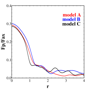
Figure 1: The ratio $Q=F_{p}/F_{ax}$ as a function of $r$, where $F_{p}$ is the maximum (with respect to the azimuth $\phi$) absolute value of the transverse force at a given cylindrical radius $r$ in the disc plane, and $F_{ax}$ is the mean absolute value (over $\phi$) of the radial force at the same radius $r$. A non-zero $Q-$ value measures the strength of the non-axisymmetric perturbation of the bar and of the spiral structure. The three curves correspond to models A (red, light gray in printed version), B (blue, gray in printed version), and C (black). The outer oscillations of the three curves are due to the spiral perturbation.

To simplify computations, we only consider the $m=2$ mode of the galactic bar. Then, the potential $\Phi(r,\phi)$ in our galactic models is given by:

$$\Phi(r,\phi)=\Phi_{0}(r)+\Phi_{1}(r)\cos 2\phi+\Phi_{2}(r)\sin 2\phi$$ (4)

where $\Phi_{0}(r)$ is the axisymmetric potential while the second and third terms of Eq.(4) correspond to an $m=2$ mode of the non-axisymmetric potential perturbation. The formulas for $\Phi_{0}(r)$, $\Phi_{1}(r)$ and $\Phi_{2}(r)$ are derived following Allen et al. (1990) and they read:

$$\Phi_{0}(r)=-\frac{1}{R}(A_{00}+\frac{1}{4}A_{20}-\frac{3}{2}A_{22})$$

$$\Phi_{1}(r)=-\frac{3}{2R}(\frac{1}{2}A_{20}+A_{22})$$ (5)

$$\Phi_{2}(r)=+\frac{3}{2R}A_{21}$$

with

$$A_{00}=\displaystyle\sum_{n=0}^{19}[B_{n00}.j_{0}(\xi_{n0})]$$

$$A_{20}=\displaystyle\sum_{n=0}^{19}[B_{n20}.j_{2}(\xi_{n2})]$$ (6)

$$A_{21}=\displaystyle\sum_{n=0}^{19}[C_{n21}.j_{2}(\xi_{n2})]$$

$$A_{22}=\displaystyle\sum_{n=0}^{19}[B_{n22}.j_{2}(\xi_{n2})]$$

where $n$ is the number of the so-called ‘radial’ terms in the series expansions of the potential, $j_{0},~{}j_{2}$ are spherical Bessel functions (see Abramowitz & Stegun (1972)) and $\xi_{nl}=a_{nl}r/R$, where $R$ is a numerical constant representing the size of the system (defined as the N-body code boundary where the solutions of the Poisson equation are matched with the solutions of the Laplace equation, see Tsoutsis et al. (2008)). Finally $a_{n0}$ are the roots of the equation $j_{n-1}(a)=0$, yielding $a_{n0}=(n+1/2)\pi$, while $a_{n2}$ are the roots of the equation $\tan(a_{n2})=a_{n2})$ (the latter are found numerically). The coefficients $B_{n00},~{}B_{n20},~{}C_{n21},~{}B_{n22}$ are calculated by the N-body code using the positions of the N-body particles and the Poisson equation $\nabla^{2}\Phi=4\pi G\rho$, where $\rho$ is the density of matter. We provide plots of the coefficients for all three galactic models in the Appendix A. The numerical values of the coefficients can be provided to any one interested after private communication.

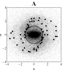
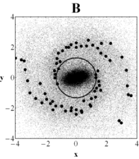
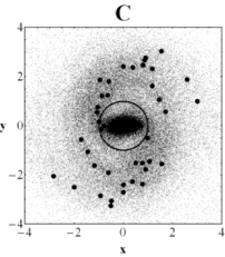
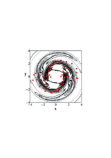
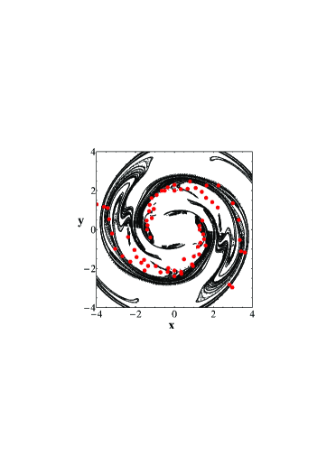
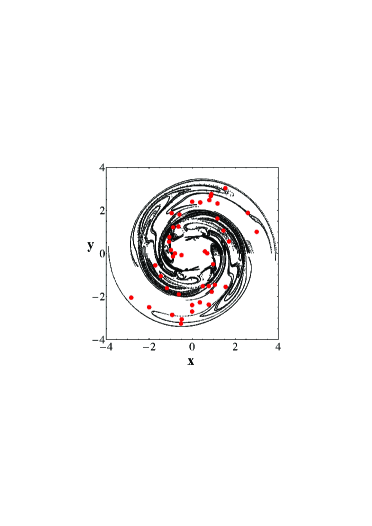
Figure 2: First line: Projection on the plane of rotation of the three N-body galactic models, ”A”, ”B” and ”C”. The circle of corotation is superimposed. The thick dots show the local maxima of the projected surface density. Second line: The numerical apocentric manifolds that track the maxima of the density for the three galactic models ”A”, ”B” and ”C” respectively. The red thick dots are the same as the black thick dots of the upper line.

In Figure 1 we plot the perturbation of each galactic model, given by the maximum ratio of the non-axisymmetric forces, due to the bar and to the spiral arms, versus total axisymmetric force, as a function of the distance $r$ for models A (red), B (blue) and C (black).

The units used in the present paper are the N-body code units. The relation of these units to natural units is discussed in detail in Tsoutsis et al. (2008). As a rough guide to figures 2,4,5,6 below, one unit of length corresponds to $\approx 8$ Kpc.

2.3 Numerical invariant manifolds

In Fig.2, in the first line we plot the three N-body galactic models at the snapshot at which we make the analysis. The circle of corotation is superimposed. The thick dots correspond to the local maxima of the surface density $\Sigma(r,\phi)$ of the N-body particles in the simulation. We find, in general, one prominent maximum along each direction and some secondary maxima. The prominent maxima always define a conspicuous spiral pattern. The secondary maxima are also observed to from patterns like spiral arms or rings. In the second line of Fig.2, now, we plot the apocentric manifolds of the $PL_{1}$ and $PL_{2}$ orbits for a Jacobi constant close to the one at $L_{1}$ (differing from it at the fourth digit). In fact, the plot consists of the first two apocenters of orbits having initial conditions along the unstable asymptotic manifold of the $PL_{1}$ and $PL_{2}$ orbits at an energy level close to the one that corresponds to the Lagrangian point $L_{1}$. Some of these results have been published already in past papers (see Voglis et al., 2006b; Tsoutsis et al., 2008) and consistently demonstrate a fact of key importance, namely that a large fraction of chaotic orbits outside corotation have many recurrences along spiral segments, i.e. they exhibit stickiness effects. Therefore they can support the spiral structure of the galaxy for considerably long times of the order of several decades of galactic periods before escaping from the system (Harsoula et al., 2011; Contopoulos & Harsoula, 2013).

In the sequel we will derive similar figures analytically, using convergent series of the normal form of the Hamiltonian for the three galactic models. We will thus establish a connection between the domain of the spiral structure and the Moser domain of convergence (see section 3.2).

3 Analytical description of the spiral arms region

In the present section, we first give the algorithm of computation of the Moser normal form around an unstable equilibrium point. We also introduce some relevant notation and terminology. Then, we implement the method in order to analytically determine the Moser domains, as well as the thereby induced loci of the spiral arms in our specific galactic models described in the previous section.

3.1 “Moser” normal form construction

(i) Hamiltonian expansion. The first step for the normal form construction is the expansion of the Hamiltonian (3) around the Lagrangian point $L_{1}$. Hamilton’s equations yield the exact position of the five Lagrangian points as the stationary points of the effective potential $\Phi_{eff}=\Phi(r,\phi)-\Omega_{p}P_{\phi}$, i.e. the solutions of the following equations:

$$\frac{dr}{dt}=\frac{\partial H}{\partial P_{r}}=0,~{}~{}\frac{dP_{r}}{dt}=-\frac{\partial H}{\partial r}=0$$

$$\frac{d\phi}{dt}=\frac{\partial H}{\partial P_{\phi}}=0,~{}~{}\frac{dP_{\phi}}{dt}=-\frac{\partial H}{\partial\phi}=0$$ (7)

Let $(r_{L_{1}},~{}P_{r_{L_{1}}},~{}\phi_{L_{1}},~{}P_{{\phi}_{L_{1}}})$ denote the solution for the Lagrangian point $L_{1}$. The radius $r_{L_{1}}$ is close to the corotation radius $r_{c}$, while the angle $\phi_{L_{1}}$ is in a direction close to the bar’s major axis. We expand the Hamiltonian (3) in series around ($r_{L_{1}},\phi_{L_{1}},P_{r_{L_{1}}},P_{{\phi}_{L_{1}}}$) by making the following substitutions:

$$r\rightarrow r_{L_{1}}+\delta r,~{}~{}P_{r}\rightarrow P_{r_{L_{1}}}+P_{x},~{}~{}\phi\rightarrow\phi_{L_{1}}+\delta\phi,~{}~{}P_{\phi}\rightarrow P_{{\phi}_{L_{1}}}+J_{\phi}$$ (8)

Since the expansion is around an equilibrium point it contains no terms linear in $(\delta r,\delta\phi,P_{x},J_{\phi})$. On the other hand, the quadratic terms $H_{2}(\delta r,\delta\phi,P_{x},J_{\phi})$ yield the linearized equations of motion around the equilibrium which are of the form

$$\left(\begin{array}[]{c}\dot{\delta r}\\ \dot{\delta\phi}\\ \dot{P_{x}}\\ \dot{J_{\phi}}\end{array}\right)=M\left(\begin{array}[]{c}\delta r\\ \delta\phi\\ P_{x}\\ J_{\phi}\end{array}\right)$$ (9)

or $\dot{X}=MX$ where $X=(\delta r,\delta\phi,P_{x},J_{\phi})^{T}$ and $M$ is the $4\times 4$ characteristic variational matrix with constant coefficients.

We now introduce a linear transformation $X=A\cdot U$ rendering the linear system (9) diagonal in a set of new canonical variables $U\equiv(\alpha,u,\beta,v)^{T}$. We require that in the new variables the linearized equations take the form $\dot{U}=\Lambda\cdot U$ where $\Lambda$ is the $4\times 4$ matrix:

$$\Lambda=\left(\begin{array}[]{cccc}\lambda_{1}&0&0&0\\ 0&\lambda_{2}&0&0\\ 0&0&\lambda_{3}&0\\ 0&0&0&\lambda_{4}\end{array}\right)$$ (10)

with $\lambda_{1}=i\omega_{0}$, $\lambda_{2}=-i\omega_{0}$, $\lambda_{3}=\nu_{0}$, $\lambda_{4}=-\nu_{0}$, being the four eigenvalues of the matrix $M$. We note that since $L_{1}$ is simply unstable it necessarily has a pair of opposite imaginary and a pair of opposite real eigenvalues. It is easy to show that the above requirements imply that the matrix $A$ contains as columns four linearly independent eigenvectors of the variational matrix $M$ corresponding to the eigevalues $\lambda_{i}$, $i=1,\ldots,4$ respectively. Each of these eigenvectors can be specified by solving the characteristic system $M\cdot A=A\cdot\Lambda$. Since this system is homogeneous the solution for each eigenvector is specified up to an arbitrary multiplicative constant. We exploit this arbitrariness in order to render the linear transformation $X\rightarrow U$ symplectic. To this end, starting from any initial solution $A$, we define a new matrix $\overline{A}$ by multiplying the first and third columns of $A$ by an unspecified coefficient $c_{1}$, and the second and fourth columns by an unspecified coefficient $c_{2}$. Finally, we specify the values of $c_{1}$ and $c_{2}$ by the requirement that the condition

$$\overline{A}~{}{\cal J}_{4}~{}\overline{A}^{T}={\cal J}_{4}$$ (11)

be satisfied, where ${\cal J}_{4}$ is the $4\times 4$ fundamental symplectic matrix

$${\cal J}_{4}=\begin{bmatrix}0&I_{2}\\ -I_{2}&0\\ \end{bmatrix}$$ (12)

where $I_{2}$ is the $2\times 2$ identity matrix. This determines the final symplectic transformation $X=\overline{A}\cdot U$.

Once the new matrix $\overline{A}$ is found we can write the expanded Hamiltonian $H$ as function of the new variables ($\alpha,u,\beta,v$), where ($\alpha,\beta$) and ($u,v$) are canonically conjugate pairs. The Hamiltonian acquires now a polynomial form:

$$H=i~{}\omega_{0}~{}\alpha~{}\beta+\nu_{0}~{}u~{}v+\sum_{s=3}^{N_{t}}P_{s}(\alpha,u,\beta,v)$$ (13)

where

$$P_{s}(\alpha,u,\beta,v)=\sum_{\stackrel{{\scriptstyle k_{1},k_{2},l_{1},l_{2}\geq 0,}}{{k_{1}+k_{2}+l_{1}+l_{2}=s}}}{\cal A}_{k_{1},k_{2},l_{1},l_{2}}\alpha^{k_{1}}u^{k_{2}}\beta^{l_{1}}v^{l_{2}}$$ (14)

are polynomials of degree $s$ with constant coefficients ${\cal A}_{k_{1},k_{2},l_{1},l_{2}}$, and $N_{t}$ is an (inevitably finite in the computer) truncation order. In all subsequent computations we set $N_{t}=20$, having checked that such an order is sufficient to accurately represent the Hamiltonian expansion in a domain of size $\sim r_{c}$ (the corotation radius) around the Lagrangian point $L_{1}$ with errors of order $10^{-8}$.

It is easy to see that the Hamiltonian (13) is of the general form (2), after the linear symplectic transformation $\alpha=(q-ip)/\sqrt{2}$, $\beta=(iq-p)/\sqrt{2}$. Thus, the complex canonical variables $(\alpha,\beta)$ still represent harmonic oscillator variables (they are known as the ‘Birkhoff variables’). Their relation to the harmonic oscillator action-angle variables $(J,\theta)$ is $\alpha=-i\sqrt{J}e^{i\theta}$, $\beta=\sqrt{J}e^{-i\theta}$. Then $J=i\alpha\beta$ is an integral of the linearized equations of motion.

(ii) Hamiltonian normalization. We now introduce a symplectic transformation of the variables $(\alpha,u,\beta,v)$ of the general form

$$\alpha = \Phi_{\alpha}(a,\xi,b,\eta)$$

$$u = \Phi_{u}(a,\xi,b,\eta)$$ (15)

$$\beta = \Phi_{\beta}(a,\xi,b,\eta)$$

$$v = \Phi_{v}(a,\xi,b,\eta)$$

aiming to render separable the Hamiltonian (13) in the new variables $(a,\xi,b,\eta)$, where ($a,b$) and ($\xi,\eta$) are canonically conjugate pairs. In particular, Moser’s theorem guarantees that there is a transformation of the form (3.1), in which the functions $\Phi_{\alpha}$, $\Phi_{u}$, $\Phi_{\beta}$, $\Phi_{v}$ are given as convergent polynomial series in a domain of the space of the new variables $(a,\xi,b,\eta)$ surrounding the origin, such that, in the new variables, the Hamiltonian becomes a function of only the products $I=iab$, $c=\xi\eta$. This new expression of the Hamiltonian $H=Z(I,c)$ is called hereafter the ‘Moser normal form’.

The details of the algebraic procedure by which we determine the transformation series (3.1) are described in detail in (Giorgilli, 2001) (see also Efthymiopoulos (2012), section 2.10, for a tutorial). Here we only summarize the formulas implementing the algorithm in the computer. Let $N_{t}$ be the maximum truncation order. The transformation for the variable $\alpha$ (and similarly for all three remaining variables in Eq.(3.1) is given by:

$$\alpha=\exp(L_{\chi_{Nt}})\exp(L_{\chi_{Nt-1}})...\exp(L_{\chi_{2}})\exp(L_{\chi_{1}})a$$ (16)

where the quantities $\chi_{r}$, $r=1,2,\ldots,N_{t}$, called the ”Lie generating functions”, are polynomial functions of degree $r+2$ in the variables $(a,\xi,b,\eta)$. The symbol $\exp(L_{\chi_{r}})$ denotes the exponential Lie operator

$$\exp(L_{\chi_{r}})=1+L_{\chi_{r}}+{1\over 2}L_{\chi_{r}}^{2}+\ldots=\sum_{n=0}^{\infty}{1\over n!}L^{n}_{\chi_{r}}$$ (17)

where $L_{\chi_{r}}$ is the Poisson bracket operator, defined for any function $g(a,\xi,b,\eta)$ by

$$L_{\chi_{r}}g={\partial g\over\partial a}{\partial\chi_{r}\over\partial b}+{\partial g\over\partial\xi}{\partial\chi_{r}\over\partial\eta}-{\partial g\over\partial b}{\partial\chi_{r}\over\partial a}-{\partial g\over\partial\eta}{\partial\chi_{r}\over\partial\xi}$$ (18)

In summary, the transformations (3.1) are found by a sequence of Poisson bracket operations on the variables $(a,\xi,b,\eta)$, which make use of certain generating functions $\chi_{r}$, specified in an appropriate way explained just below. In the computer, we truncate any repeated Poisson bracket operation at the point where the operation starts yielding terms of degree higher than $N_{t}+2$. This yields eventually a finite truncation of each of the four series of Eq.(3.1).

The functions $\chi_{r}$, now, are specified step by step by a recursive algorithm. Let $H^{(0)}(a,\xi,b,\eta)\equiv H(a,\xi,b,\eta)$. Assume that $r$ steps of the algorithm were completed. The $r^{th+1}$ function $\chi_{r+1}$ is the solution of the equation

$$\{i\omega_{0}ab+\nu_{0}\xi\eta,\chi_{r+1}\}+h^{(r)}_{r+1}=0$$ (19)

where $h^{(r)}_{r+1}$ is a polynomial function of degree $r+3$ which contains all the monomial terms of the function

$$H^{(r)}=\exp(L_{\chi_{r}})\exp(L_{\chi_{r-1}})...\exp(L_{\chi_{2}})\exp(L_{\chi_{1}})H^{(0)}$$ (20)

which are of form $c_{k_{1},k_{2},l_{1},l_{2}}a^{k_{1}}\xi^{k_{2}}b^{l_{1}}\eta^{l_{2}}$ such that $k_{1}+k_{2}+l_{1}+l_{2}=r+2$ and $k_{1}\neq l_{1}$ or $k_{2}\neq l_{2}$. The solution of Eq.(19) is straightforward. Namely, the solution is found by the rule:

$$\mbox{For every term~{}}c_{k_{1},k_{2},l_{1},l_{2}}a^{k_{1}}\xi^{k_{2}}b^{l_{1}}\eta^{l_{2}}\mbox{~{}in~{}}h^{(r)}_{r+1}$$

$$\mbox{add the term~{}}{c_{k_{1},k_{2},l_{1},l_{2}}a^{k_{1}}\xi^{k_{2}}b^{l_{1}}\eta^{l_{2}}\over i(k_{1}-l_{1})\omega_{0}+(k_{2}-l_{2})\nu_{0}}\mbox{~{}in~{}}\chi_{r+1}$$

Thus, the whole scheme of the computation of the Moser normal form becomes a sequence of basically trivial algebraic operations, i.e. multiplication or division by constants and computations of Poisson brackets for polynomial functions. Let us note that the convergence of the series is based on the fact that the method introduces divisors of the form $im_{1}\omega_{0}+m_{2}\nu_{0}$, with $(m_{1},m_{2})$ integers, which can never become very small.

(iii) Normal form dynamics. The final expression of the Moser normal form is the Hamiltonian function $Z(a,\xi,b,\eta)=H^{(N_{t})}(a,\xi,b,\eta)$. This function has the form:

$$Z(I=iab,c=\xi\eta)=i\omega_{0}ab+\nu_{0}\xi\eta+\zeta_{21}a^{2}b^{2}+\zeta_{22}\xi^{2}\eta^{2}$$

$$+\zeta_{23}ab\xi\eta+\zeta_{31}a^{3}b^{3}+\zeta_{32}ab\xi^{2}\eta^{2}$$

$$+\zeta_{33}q^{2}p^{2}\xi\eta+\zeta_{34}\xi^{3}\eta^{3}+...$$ (21)

with terms depending on powers of the products $I=iab,c=\xi\eta$ up to order $N_{t}/2+1$ (for symmetry reasons in the original Hamiltonian $N_{t}$ has to be chosen even). By Hamilton’s equations we trivially find $\dot{I}=\dot{c}=0$. Thus, both quantities $(I,c)$ represent integrals of motion under the normal form dynamics. In contrast to what happens with the usual Birkhoff series (see Contopoulos 2002 for a review), we emphasize that the integrals $I,c$ in the above computation are not only formal. In fact, the series giving them are convergent. Thus, the integrals represent true invariants of motion, whose precision of computation within the Moser domain of convergence depends only on the level of the series truncation. The physical meaning of these integrals is the following:

(a) The integral $I$ is given by $I=J+$higher order terms, where, as noted above, $J$ is the action integral of the harmonic oscillator in the elliptic degree of freedom of the linearized equations of motion. Being produced by the full equations of motion, $I$ is the action integral of a nonlinear oscillation, which, as explained in section 2, represents an independent oscillation taking place in the center manifold of the unstable equilibrium point $L_{1}$. If we set $\xi=\eta=0$, one such oscillatory solution corresponds to one member of the short-period orbit around the point $L_{1}$. Thus, $I$ is a label of the whole family of these orbits, with an increasing value of $I$ representing an increasing size of the epicycle described by the short-period orbit around $L_{1}$. In particular, the value $I=0$ represents the limit when the size of the epicycle reduces to zero, i.e., the Lagrangian point $L_{1}$ itself.

(b) The integral $c=\xi\eta$ yields a family of invariant hyperbolae in the plane $(\xi,\eta)$. Consider a fixed value of $I$. For every point $(\xi,\eta)$ within the Moser domain of convergence, using the transformation equations (3.1) we can find a corresponding point in the original variables. Then, the points on one invariant hyperbola are mapped on points on an invariant curve in the phase space of the original variables. This curve is hereafter called a ‘Moser invariant curve’. Such curves characterize the structure of chaotic orbits in the vicinity of the unstable equilbrium. In particular, all the chaotic orbits have their consequents arranged along such curves (see Efthymiopoulos et al. (2014); Harsoula et al. (2015); Contopoulos & Harsoula (2015) for a detailed discussion of the properties of the Moser curves in simple dynamical systems). Of particular importance is the value $c=0$. Then, one Moser curve splits in three parts, namely (1) the invariant point $\xi=\eta=0$, i.e., the fixed point of a short-period orbit, (2) the $\xi-$axis ($\eta=0$), i.e., the unstable manifold, and (3) the $\eta-$axis ($\xi=0$), i.e., the stable manifold of the short-period orbit. These are reduced to the fixed point and stable and unstable manifolds of the Lagrangian point $L_{1}$ itself for $I=0$.

After the above definitions, we discuss now our main result, namely the connection between the Moser domain of convergence and the chaotic spiral arms in our galactic models.

3.2 Moser domain of convergence

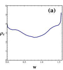
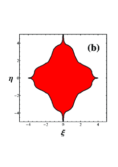
Figure 3: (a) The radius of convergence of the series (3.1) as a function of the angle $w$ for $w=0$ to $w=\pi/2$.(b) The region of convergence on the ($\xi,\eta$) plane. Both (a) and (b) correspond to the galactic model ”C”.

In the sequel, we focus on the case $I=0$, i.e., the computation of the Moser domain of convergence around the Lagrangian point $L_{1}$ itself. However, the same method can be applied to any case with $I\neq 0$.

Setting $a=b=0$ in the transformation series (3.1), all four series become polynomial in the two variables $(\xi,\eta)$. In order to compute the domain of convergence we now work with a variant of the method introduced in a previous paper (Contopoulos & Harsoula, 2015). From Eq.(3.1), taking, as an example, the truncated series $\Phi_{u}(a=0,b=0,\xi,\eta)$, we have

$$\Phi_{u}(a=0,b=0,\xi,\eta)=\sum_{s=1}^{N_{t}+2}\sum_{k=0}^{s}f_{s,k}\xi^{k}\eta^{s-k}$$ (22)

Define now a particular direction in the $(\xi,\eta)$ plane passing through the origin, parameterized by the equations $\xi=\rho\cos w$, $\eta=\rho\sin w$, with $w$ fixed. Then, the integral $c=\xi~{}\eta$ (see previous subsection) becomes $c=\rho^{2}\cos w\sin w$. Substituting these expressions in the series (22), we obtain a series depending only on powers of the distance $\rho$ from the origin:

$$\Phi_{u}(\rho;w)=\sum_{s=1}^{N_{t}+2}B_{s}(w)\rho^{s}$$ (23)

with

$$B_{s}(w)=\sum_{k=0}^{s}f_{s,k}\cos^{k}(w)\sin^{s-k}(w)$$ (24)

We define the sequence of ‘Cauchy radii’, depending on the integer $s=1,2,...$ by

$$\rho_{\textrm{c,s}}(w)=|1/B_{s}(w)|^{1/s}$$ (25)

According to the Cauchy theorem, the series (23) converges inside the radius $\rho_{\textrm{c}}(w)=\lim_{s\rightarrow\infty}\rho_{c,s}(w)$. In practice, since we work with a finite truncation, we compute the sequence (25) and check numerically that it converges to a nearly constant value for large $s$. Introducing also a 0.95 safety factor, we define a numerical estimate of the convergence radius as

$$\rho_{\textrm{c,num}}(w)=0.95\rho_{c,N_{t}+2}(w)$$ (26)

with $N_{t}=20$ in all computations below.

Figure 3a shows an example, for the galactic model $"C"$, of the numerically computed radius of convergence $\rho_{\textrm{c,num}}$ as a function of the angle $w$ where $w\in[0,\pi/2]$. Figure 3b shows the domain of convergence (red) inside the limiting black curve corresponding to the radius of convergence for all four quadrants in the same example. Let us point out that any one of the four series of Eq.(3.1) can be used in the computation of the convergence domain, since, by the series construction, all transformations should converge within the same domain.

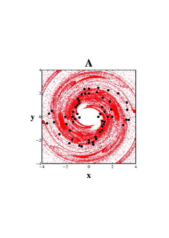
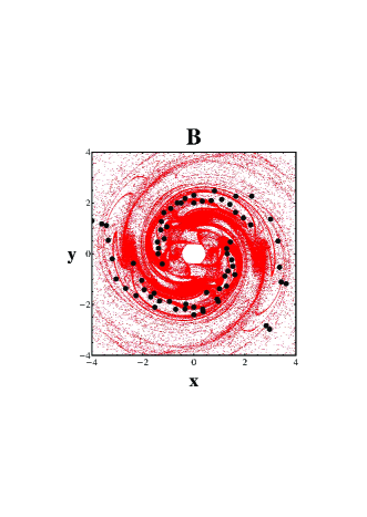
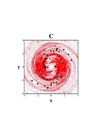
Figure 4: The extended Moser domains of convergence ${\cal M}_{ext}$ (see text), for our three galactic models $"A"$, $"B"$ and $"C"$, in the configuration space of the galaxy. We plot the first three apocenters of each orbit with random initial condition inside the Moser domain of convergence ${\cal M}$ (like the one of Fig. 3b). One can identify spiral arms, in all three galactic models, which are consistent with the local maxima of the projected surface density of the N-body particles (black dots). The dots are the same as in Fig.2.

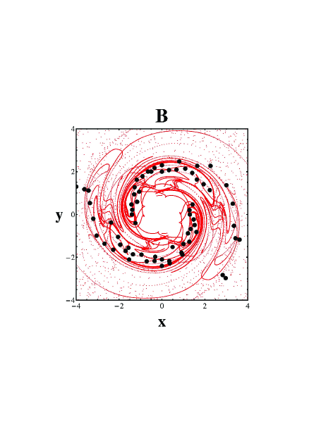
Figure 5: Left: We plot the first three images on the apocentric surface of section, of the initial conditions along the $\xi$-axis of the Moser domain of convergence (which corresponds to the unstable asymptotic curve of the $L_{1}$ (and its symmetric $L_{2}$) point together with the local maxima of the projected surface density of the N-body particles (black dots). Right: same as in the left panel but for the pericentric surface of section ($\dot{r}=P_{r}=0$, $\dot{p}_{r}>0$).

Note that the present case is somewhat different from the cases considered previously in Harsoula et al. (2015) and Contopoulos & Harsoula (2015). Namely, in those studies it was found numerically that the limiting value of $c=c_{\textrm{lim}}$ (see (iii) of subsection 3.1 for the definition of $c$), was independent of the angle $w$. Here, instead, we find that $c$ depends on $w$ so that the boundary of the Moser domain differs from a pure hyperbola. In particular, we find that $\rho_{\textrm{c}}$ is finite in both axes $\xi=0$ and $\eta=0$. The origin of this difference is due to a difference between the convergence domains in the case of real analytic mappings on the plane, and systems, like the present one, produced by a continuous Hamiltonian flow (see Efthymiopoulos et al. (2014)).

Figure 4 shows now the main result. It is produced as follows: We construct a set of randomly distributed initial conditions inside the Moser domain of convergence in the ($\xi,\eta$) plane (as in Fig.3b). Using the transformation equations (3.1), with $a=b=0$, as well as the linear transformation $\overline{A}$ of section 2, every one of these points can be mapped to a point in the original canonical variables $(r,\phi,P_{r},P_{\phi})$ and eventually in the cartesian variables ($x,y,p_{x},p_{y}$). This process defines the image of the Moser domain in the phase space of the original variables. This is hereafter called ${\cal M}$.

Every initial condition in $\cal{M}$, when integrated forward in time, reaches consecutive apocentric positions of the orbit, at some times $t=t_{1},t_{2},...$. Hereafter, we call apocentric surface of section the surface defined by the relation $\dot{r}=P_{r}=0$, $\dot{p}_{r}<0$. We note that this is a 2D surface of section embedded in the 4D phase space. In subsequent plots we focus on the projection of this surface in the usual configuration space ($x=r\cos(\phi)$, $y=r\sin(\phi)$).

Following, now, da Silva Ritter et al. (1987) (see also Efthymiopoulos et al. (2014)), we hereafter call the extended Moser domain in the plane $(\xi,\eta)$ the union of the original Moser domain of Fig.3b along with all its forward images at the times $t_{1},t_{2},...$. The latter can be computed analytically, given the normal form of Eq.(3.1). This process allows to establish an extension of the transformations of Eq.(3.1) from the plane $(\xi,\eta)$ to the configuration space $(x,y)$. The extended Moser domain is found by propagating forward in time all the grid points in ${\cal M}$. The propagation can be done analytically using a so-called “extended method” developed in Efthymiopoulos et al. (2014), but here, for simplicity, we simply perform it by numerical integration of the orbits.

We hereafter denote by ${\cal M}_{ext}$ the image of the extended Moser domain on the plane $(x,y)$. Figure 4 shows the intersection of ${\cal M}_{ext}$ with the apocentric surface of section $\dot{r}=0$, $\dot{p}_{r}<0$, with a computation of ${\cal M}_{ext}$ up to a time covering three apocentric passages for all the orbits in ${\cal M}$. The reason for this choice of the apocentric section is that ${\cal M}_{ext}$ in this section contains the apocentric sections of the unstable manifolds of $L_{1}$ and their neighborhoods.

As shown clearly in Fig.4, the images of the Moser domains of convergence in the configuration space of all three models define areas on non-zero measure which have the forms of spiral arms, which are consistent with the images of the local maxima of the projected surface densities of the N-body particles (black dots). In fact, a careful inspection of all three panels in Fig.4 reveals that there are domains where distinct parts of ${\cal M}_{ext}$ overlap. This is allowed since the transformation (3.1) is not bijective. Actually, the greatest enhancement of the spiral densities occurs, precisely, in domains of such overlapping.

It is emphasized that both the N-body particles forming the spiral arms as well as fictitious particles with initial conditions in the set ${\cal M}_{ext}$ move along chaotic orbits. A theoretical interpretation of the role of ${\cal M}_{ext}$ in determining the dynamics along the chaotic spirals is given in the next section.

In Fig.5 we plot the images of initial conditions along the $\xi$-axis of the Moser domain of convergence, for the galactic model ”B”. The images of these initial conditions correspond to the unstable asymptotic curves of the equilibrium points $L_{1}$, $L_{2}$. In the left panel of figure 5 we plot the first three apocenters (red dots) of the unstable asymptotic curves, superposed to the local density maxima of the N-body particles (thick black dots). Note that, besides the main spiral structure, these plots indicate that the manifolds support also a second pair of spiral arms nearly parallel to the main spiral arms. A similar result was found in a previous paper using orbital structure study (see Fig. 20 of Contopoulos and Harsoula 2013.) Let us note that the ”double spiral” structure, is a notable morphological feature in many barred-spiral galaxies.

In the right panel of figure 5 we plot the pericenters of the unstable asymptotic curves from $L_{1}$ and $L_{2}$, which support the limit of the bar and the innermost part of the spiral structure.

4 Theoretical interpretation

A typical property of all galactic dynamical systems with a strong bar is that the phase space beyond corotation is open to escapes. Numerical simulations show that most stars in chaotic orbits acquire escape velocities from the galaxy in rather short timescales (of the order of a few dynamical periods only). On the other hand, the stars with initial conditions close to the phase-space invariant structures such as invariant manifolds or cantori are ”sticky”, i.e they resist in general the escaping flow for longer times, which are often sufficient to support structures such as chaotic spiral arms.

Our interpretation of the role that the Moser domains play in the phenomenon of chaotic spirals is based on the findings in the recent work of Contopoulos & Harsoula (2015). In this work, the following two properties were demonstrated:

i) All the chaotic orbits with initial conditions inside a Moser domain of convergence remain bounded within the extended Moser domain for arbitrarily long times. This property is a consequence of the Moser normal form dynamics. Namely, the successive consequents of the chaotic orbits with initial conditions within the Moser domain necessarily lie in one invariant Moser curve (i.e. a hyperbola $\xi\eta=c$ in the $(\xi,\eta)$ plane and its image in the configuration plane).

ii) The boundary of the Moser domain acts as an attractor for all the chaotic orbits with initial conditions outside but close to it, although these orbits escape asymptotically to infinity. This property implies that the chaotic escapes do not take place in random directions in phase space, but the successive consequents of the escaping orbits necessarily approach closer and closer to the boundaries of one or more Moser domains (formed around one or more unstable periodic orbits in the same system, see Contopoulos & Harsoula (2015)). As a result, the preferential directions of escape for all the orbits are those along which the Moser domains of the unstable periodic orbits extend to infinity.

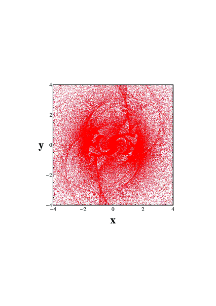
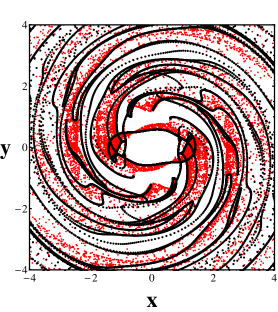
Figure 6: Left: The projection on the configuration plane of the galactic model ”B” of orbits whose initial conditions on the $(\xi,\eta)$ plane, are inside the grid ($-5<\xi<5$,$-5<\eta<5$), but outside the Moser region of convergence (red region of Fig. 3). Right: The first apocentric positions of the orbits of (a) together with the first apocenter of the image of the boundary of the Moser domain of convergence of Fig. 3 (black curve). These chaotic orbits will finally escape with a slow diffusion along spirals.

The above results were found in simple area-preserving mappings, but we now show how they translate in the case of the Moser domains ${\cal M}_{ext}$ computed in our galactic models. Figure 6 summarizes the relevant information. The left panel of Fig. 6 gives the projection on the configuration space of the galactic model ”B”, of orbits whose initial conditions on the $(\xi,\eta)$ plane are inside a grid ($-5<\xi<5$,$-5<\eta<5$), but outside the Moser domain of convergence (red region of Fig. 3). Using the transformation equations (3.1), with $a=b=0$, as well as the linear transformation $\overline{A}$ of section 2, we map these points in the original canonical variables $(r,\phi,P_{r},P_{\phi})$ and eventually in the cartesian variables ($x,y,p_{x},p_{y}$). Using these initial conditions, we then integrate the orbits until they reach their first apocentric section (we only consider the orbits which have initially a negative energy in the inertial frame, i.e. $E=0.5(P^{2}_{r}+P^{2}_{\phi}/r^{2})+V(r,\phi)<0$, since the orbits with $E>0$ escape from the system immediately). The so-resulting distribution of the orbits in the apocentric section is shown in the right panel of Fig. 6, together with the image , in the same section, of the boundary of the Moser domain (black curve).

We observe that the boundary of the Moser domain ${\cal M}_{ext}$ attracts all the exterior orbits in its neighborhood. These orbits follow escaping paths close to this boundary, along the spiral pattern. In fact, this spiral makes several revolutions as shown in Fig.6b. However the density of points falls (nearly exponentially) as the distance from the center increases, thus practically limiting the extent along which the spiral arms are traced by an appreciable amount of matter.

On the other hand, we may note that a clear, albeit only qualitatively correct, theoretical picture can be obtained by constructing an approximate explicit mapping model to represent the dynamics in the corotation region around the Lagrangian points. We close our analysis in this paper by showing results based on such an approximate mapping, which we constructed using a method borrowed from solar system studies (the so-called ‘Hadjidemetriou method’ (Hadjidemetriou, 1991, 2008)). Deferring all technical details of the mapping construction to Appendix B, we here summarize only the final result. By constructing a so-called “averaged Hamiltonian” based on the epicyclic approximation applied to the potential of each N-body galactic model, we end up by showing that the dynamics around the Lagrangian points $L_{1}$ and $L_{2}$ can be approximated by a version of the well known Chirikov standard map (Chirikov, 1979):

$$~{}~{}~{}~{}~{}~{}~{}~{}~{}~{}~{}~{}~{}\Theta^{\prime}=~{}\Theta+Y^{\prime}$$

$$~{}~{}~{}~{}~{}~{}~{}~{}~{}~{}~{}~{}~{}Y^{\prime}=Y+K\sin(\Theta)$$ (27)

where $K$ is a non-linearity parameter depending on the perturbation of each galactic model. The variables $(\Theta,Y)$ in the mapping (4) are connected to cylindrical coordinates via the azimuth $\phi$ and its conjugate action $J_{\phi}$, which measures the distance away from corotation ($J_{\phi}>0$ outside corotation and $J_{\phi}<0$ inside corotation). The value of the non-linearity parameter $K$ is proportional to the strength of the $m=2$ component of the potential at corotation. The value of $K$ derived for the three different models considered is $K_{A}=2.7$ (model $"A"$), $K_{B}=4.6$ (model $"B"$) and $K_{C}=9.3$ (model $"C"$) (see Appendix B for details). Thus, in all three models the non-linearity is quite strong, and results in a phase space where most chaotic orbits are free to escape.

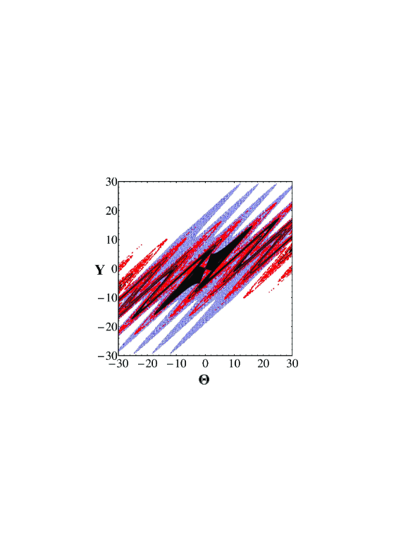
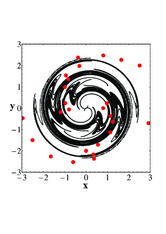
Figure 7: (a) The successive iterations of a grid of points outside the region of convergence (black region) of the standard map (4) for the galactic model ”A”. Blue is the first and red is the third iteration of this region. It is obvious that the successive iterations get closer and closer to the black region of convergence. In fact, the outer boundary of the Moser region of convergence acts like an attractor in the phase space. (b) The Moser domain of convergence (black region of (a)) in the configuration space of the galactic model $A$, superimposed with the local maxima of the projected surface density (red dots). It’s obvious that the spiral arms of the mapping approximation are more tightly wounded than the ones of the galactic model.

The Lagrangian points $L_{1}$, $L_{2}$, or the fixed points of the family of the short-period orbits $PL_{1}$, $PL_{2}$, correspond to the hyperbolic point $(\Theta=0,Y=0)$ (or $(2\pi,0)$ which is the same point modulo $2\pi$). Using the same formulas for the production of the Moser normal form for area-symplectic mappings as in (Contopoulos & Harsoula, 2015), we compute the Moser domain of convergence of the mapping (4) first in the mapping variables $(\Theta,Y)$, and then in the original cylindrical canonical variables of our galactic models.

Figure 7a shows an example of the Moser domain of convergence (black) in the mapping variables $(\Theta,Y)$, for the galactic model $"A"$. Also, taking a set of initial conditions outside the Moser domain, the same plot shows their first (blue) and third (red) iterations in the same plane. It is obvious that the successive mappings of the initial conditions outside the Moser domain of convergence come closer and closer to the boundary of the (black) domain of convergence. However, these orbits can only approach asymptotically the boundary of the domain, and they cannot enter inside the the black domain. Hence, the boundary of the Moser domain acts like an attractor in the phase space for all the orbits with initial conditions outside the Moser domain. These orbits finally escape to infinity. In fact the boundary of the Moser domain (black) forms an infinity of oscillations beyond the limits of Fig.7a. Thus the orbits outside and close this boundary extend to arbitrarily large ($\Theta$) and the corresponding spirals of Fig. 7b extend to arbitrarily large distances.

Finally, Fig.7b shows the image of Fig.7a in the configuration space of the galactic model $"A"$. Thus, Fig.7 gives the same results as Fig.6, but depicts more clearly the attraction of the escaping orbits by the boundary of the Moser domain. Note that also in this simple mapping model, the Moser domain exhibits a spiral form. However, we stress that the mapping model (4) only serves for a theoretical interpretation of previous results, while its comparison with the exact model can only be qualitative. In fact, the spiral structure in Fig.7b appears more tightly wound than the true spiral structure of the model (red dots).

Similar results were found also in the models $"B"$ and $"C"$.

5 Conclusions

In the present paper we demonstrate a close connection between the form of the chaotic spiral arms in barred galaxies and an analytical theory describing the chaotic orbits in the neighborhood of the unstable points $L_{1}$ and $L_{2}$ at the end of bars due to Moser (1956, 1958). Our present results complement in an essential way the manifold theory of spiral structure (Voglis et al., 2006b; Romero-Gomez et al., 2006), and they allow to build analytically domains of non-zero measure in phase space which correspond to a non-zero phase space density of stars moving along the spiral arms. In particular:

1) We computed the so-called ’Moser normal form’ (see section 3), i.e. a convergent series of perturbation theory allowing to characterize analytically the chaotic orbits with initial conditions in the neighborhood of the invariant manifolds of the unstable points $L_{1}$ or $L_{2}$. We gave particular examples of Moser normal form computations based on potential models derived by N-body simulations of barred-spiral galaxies.

2) We computed the domain of convergence of the Moser series in the normal form variables, and found its image in the usual configuration space of the disc plane. This image, in all three galactic models has the form of trailing spiral arms, which can be computed analytically knowing only the coefficients of the potential expansion. We emphasized that when the orbits within a Moser domain are recurrent, the spiral structure is formed by the intersection of the domain of convergence with a so-called ‘apocentric’ section (see section 3).

3) We computed the local maxima of the surface density on the disc for the real N-body particles and verified their good agreement with the analytically computed spirals.

4) We gave a theoretical interpretation of this agreement (section 4) based on findings in previous works (Harsoula et al., 2015; Contopoulos & Harsoula, 2015) regarding the dynamical role of the Moser domains in the stickiness and escape dynamics in simple mappings with a phase space open to escaping chaotic motions. We demonstrate that the boundaries of the Moser domains of convergence act as attractors for the escaping chaotic orbits with initial conditions near, but in the exterior of this domain. On the other hand, all the chaotic orbits with initial conditions inside a Moser domain necessarily reproduce the spiral form of this domain, since they can never escape outside this domain.

5) Finally, we constructed a simple mapping of the type of Chirikov’s standard map, based on the averaged-Hamiltonian approach of Hadjidemetriou (1991, 2008), which allows to reproduce qualitatively the apocentric section dynamics of the chaotic orbits in the neighborhood of $L_{1}$ or $L_{2}$. The Moser domain of convergence extends to infinity along the invariant manifolds of the mapping’s unstable fixed point at the origin. Thus, the geometric loci of the corresponing spiral arms in the galactic plane extend to infinity. However, the density of matter falls exponentially along these loci, hence, the Moser theory leads to theoretical spiral arms of only a finite extent beyond the corotation region.

Appendix A: The coefficients of the galactic potentials

The coefficients of Eq. (2.2) of the potential $\Phi(r,\phi)$ for the three galactic models $A$, $B$ and $C$ that are plotted in Fig.8.

The 20 coefficients $B00$ correspond to monopole terms, the 20 coefficients $B20$ to quadrupole terms and the remaining 80 coefficients $B21,~{}C21,~{}B22,~{}C22$ to triaxial terms. Values are given in the N-body units (see Voglis et al. (2006a)). In the same units one has $R=0.85$, while the corresponding pattern speeds are: $\Omega_{pA}=5886.65$, $\Omega_{pB}=6010.36$, $\Omega_{pC}=6137.14$ (corresponding to $\approx 20-25~{}km~{}sec^{-1}~{}Kpc^{-1}$ in physical units). Length units in Figures 1,2,4,5,6,7b were rescaled by the half mass radius ($R_{hm}$) of each galactic model, i.e. by a factor of 0.1006, 0.0926 and 0.1167 for models ”A”, ”B” and ”C”, respectively.

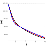
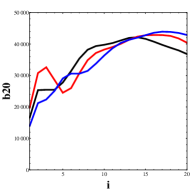
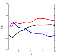
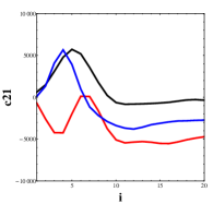
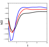
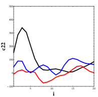
Figure 8: The coefficients of the potential of Eq.(4) for the three galactic models. Black (light gray in the printed version), red(gray in the printed version) and blue (black in the printed version) curves correspond to model $"A"$, $"B"$ and $"C"$, respectively.

Appendix B: Construction of an approximate mapping at corotation

We show below how to construct an approximate symplectic mapping describing the motion of stars at the corotation resonance, based on the epicyclic approximation.

The corotation radius $r_{c}$ is the root for $r$ of the equation:

$$\Omega_{p}=\sqrt{F_{0}/r}$$ (28)

where $F_{0}=\partial\Phi_{0}(r)/\partial r$ is the axisymmetric force. The angular momentum at corotation is $P_{\phi c}=\Omega_{p}r_{c}^{2}$. We define the quantities

$$J_{\phi}=P_{\phi}-P_{\phi c},~{}~{}~{}~{}~{}~{}\delta r=r-r_{c}$$ (29)

Substituting (29) in Eq.(3), the Hamiltonian becomes a function of the new variables $H=H(J_{\phi},\phi,P_{r},\delta r)$, which is polynomial of order 2 in $J_{\phi}$. We also make a series expansion up to order 4 in $\delta r$. Then, the Hamiltonian takes the form:

$$H=\frac{1}{2}P^{2}_{r}+\frac{1}{2}\kappa^{2}_{r}\delta r^{2}+\frac{J^{2}_{\phi}}{2r_{c}^{2}}-(2P_{\phi c}/r_{c}^{3})J_{\phi}\delta r$$

$$+(3P_{\phi c}/r_{c}^{4})J_{\phi}\delta r^{2}-(1/r_{c}^{3})J^{2}_{\phi}\delta r+(3/2r_{c}^{4})J_{\phi}^{2}\delta r^{2}$$ (30)

$$+A_{1}\cos(2\phi)+A_{2}\sin(2\phi)+B_{1}\delta r\cos(2\phi)+B_{2}\delta r\sin(2\phi)$$

$$+C_{1}\delta r^{2}\cos(2\phi)+C_{2}\delta r^{2}\sin(2\phi)+{\cal O}(\delta r^{3})+{\cal O}(\delta r^{4})+\ldots$$

In Eq.(Appendix B: Construction of an approximate mapping at corotation) $\kappa_{r}$ is the epicyclic frequency at corotation

$$\kappa_{r}=\sqrt{\frac{\partial^{2}\Phi_{eff}(r)}{\partial r^{2}}}\Large{|}_{r_{c}}$$ (31)

where $\Phi_{eff}=\frac{P^{2}_{\phi c}}{2r^{2}}+\Phi_{0}(r)$ is the effective potential of the axisymmetric component. The constants $A_{1}$, $A_{2}$, $B_{1}$, $B_{2}$, $C_{1}$, $C_{2}$ are computed from the general expansion of the potential evaluated at the corotation radius.

We now introduce a pair of epicyclic action-angle variables $(J_{r},\phi_{r})$ via the relations:

$$\delta r=\sqrt{\frac{2J_{r}}{\kappa_{r}}}\sin(\phi_{r}),~{}~{}~{}P_{r}=\sqrt{2\kappa_{r}J_{r}}\cos(\phi_{r})$$ (32)

The lowest order terms of the Hamiltonian (Appendix B: Construction of an approximate mapping at corotation) take the form:

$$H=\kappa_{r}J_{r}-(2P_{\phi c}/r_{c}^{3})J_{\phi}\sqrt{\frac{2J_{r}}{\kappa_{r}}}\sin(\phi_{r})$$

$$+\frac{J^{2}_{\phi}}{2r_{c}^{2}}+A_{1}\cos(2\phi)+A_{2}\sin(2\phi)+...$$ (33)

The above Hamiltonian can be ‘averaged’ over the fast angle $\phi_{r}$, i.e. the epicyclic phase. The averaging introduces a correction of the reference radius $r_{0}$ around which the epicyclic approximation is implemented, with respect to the radius of the circular orbit $r_{c}$ at corotation (see Contopoulos, 2002, p.381). We use the Lie method in order to make this correction via a canonical transformation. Thus, we define the new Hamiltonian

$$H^{\prime}=\exp(L_{X_{1}})H=H+L_{X_{1}}H+\frac{1}{2}L^{2}_{X_{1}}H+...$$ (34)

where $L_{X_{1}}\equiv\{{\cdot,X_{1}\}}$ is the Poisson bracket operator, and

$$X_{1}=-(2P_{\phi c}/\kappa_{r}r_{c}^{3})J_{\phi}\sqrt{\frac{2J_{r}}{\kappa_{r}}}\cos(\phi_{r})$$ (35)

The new averaged Hamiltonian has the form:

$$H^{\prime}=H(\phi,J_{\phi},J_{r})=\kappa_{r}J_{r}+B_{1}J_{r}^{2}+B_{2}J_{r}J_{\phi}+B_{3}J^{2}_{\phi}$$

$$+B_{4}J_{r}J^{2}_{\phi}+B_{5}\cos(2\phi)+B_{6}J_{r}\cos(2\phi)+$$

$$B_{7}\sin(2\phi)+B_{8}J_{r}\sin(2\phi)+\ldots$$ (36)

where i) $B_{s}$ are known coefficients, and ii) all higher-order terms depending on the fast angle $\phi_{r}$ are ignored.

In the approximation of the Hamiltonian (Appendix B: Construction of an approximate mapping at corotation) $J_{r}$ is an integral of motion, corresponding to a nearly constant value of the epicyclic action along the epicyclic oscillations. On the other hand, the variables $(\phi,J_{\phi})$ yield a pendulum-like behavior, characteristic of the corotation resonance. We will now use the Hadjidemetriou method in order to obtain a symplectic mapping model better describing this resonance. According to this method, the averaged Hamiltonian $H^{\prime}(J_{r},\phi,J_{\phi})$ is employed in order to define a generating function $S$ of the second kind:

$$S=\phi J^{\prime}_{\phi}+T_{r}H^{\prime}(J_{r},\phi,J^{\prime}_{\phi})$$ (37)

where $T_{r}=2\pi/\kappa_{r}$ is the epicyclic period. The symplectic mapping equations are then given by:

$$~{}~{}~{}~{}~{}~{}~{}~{}~{}~{}~{}~{}~{}~{}~{}~{}~{}~{}~{}~{}~{}J_{\phi}=\frac{\partial S}{\partial\phi}=G(\phi,J_{r},J^{\prime}_{\phi})$$

$$\phi^{\prime}=\frac{\partial S}{\partial J^{\prime}_{\phi}}=F(\phi,J_{r},J^{\prime}_{\phi})$$ (38)

Solved for $\phi^{\prime}$, $J_{\phi}^{\prime}$, these equations give the mapping $(\phi,J_{\phi})\rightarrow(\phi^{\prime},J_{\phi}^{\prime})$ after one epicyclic period. The variable $J_{r}$ is a constant parameter of the mapping. In particular, the value $J_{r}=0$ corresponds to orbits with a zero epicyclic oscillations, i.e., asymptotic to the Lagrangian points $L_{1}$, $L_{2}$, while for $J_{r}\neq 0$ we find orbits asymptotic to the short period orbits $PL_{1}$ or $PL_{2}$.

Setting $J_{r}$=0 we have the expressions of $J^{\prime}_{\phi}$ and $\phi^{\prime}$:

$$~{}~{}~{}~{}~{}~{}~{}~{}~{}~{}~{}J^{\prime}_{\phi}=J_{\phi}+C_{1}\cos(2\phi)+C_{2}\sin(2\phi)$$

$$\phi^{\prime}=\phi+C_{3}J_{\phi}+C_{4}\cos(2\phi)+C_{5}\sin(2\phi)$$ (39)

with $C_{1},...C_{5}$ known coefficients.

It is straightforward to show that the mapping (Appendix B: Construction of an approximate mapping at corotation) takes the form of the well known Standard map (Chirikov, 1979) after some appropriate transformations which include the following: (a) Eliminate the $\cos(2\phi)$ term, (b) eliminate the factor 2 inside the $\sin$ term and (c) eliminate the coefficient $C_{3}$ of the $J_{\phi}$ term.

Non-zero coefficients $C_{1},~{}C_{4}$ indicate that the main axes of the bar of the galaxy are not aligned with the axes $(x,~{}y)$ of the coordinate system. We find the bar’s axis angular position by calculating the coordinates of the main periodic orbits of the mapping (Appendix B: Construction of an approximate mapping at corotation). The system of equations:

$$J^{\prime}_{\phi}=J_{\phi},~{}~{}~{}\phi^{\prime}=\phi$$ (40)

gives the solution $J_{\phi}=0$ and $\phi=\pi/2+\delta\phi$. Making for some constant $\delta\phi$ the transformation $\phi\rightarrow\theta+\delta\phi$ the mapping (Appendix B: Construction of an approximate mapping at corotation) takes the form:

$$~{}~{}~{}~{}~{}~{}~{}~{}~{}~{}~{}~{}~{}~{}~{}x_{v}=C^{\prime}_{1}J_{\phi}+\theta+C^{\prime}_{2}\sin(2\theta)$$

$$y_{v}=J_{\phi}+C^{\prime}_{3}\sin(2\theta)$$ (41)

Finally making the transformation $\theta\rightarrow\Theta/2$ and $J_{\phi}\rightarrow Y/(2C^{\prime}_{1})$ we arrive at the standard map:

$$~{}~{}~{}~{}~{}~{}~{}~{}~{}~{}~{}~{}~{}~{}~{}~{}~{}\Theta^{\prime}=\Theta+Y+K\sin(\Theta)$$

$$Y^{\prime}=Y+K\sin(\Theta)$$ (42)

$K$ is a non linearity parameter depending on the non-axisymmetric perturbation of the galactic model.

One way to quantify how good is the mapping approximation (Appendix B: Construction of an approximate mapping at corotation) is by comparing the eigenvalues of its unstable periodic orbits with the ones derived from the original Hamiltonian.

Taylor expanding the Hamiltonian (Appendix B: Construction of an approximate mapping at corotation) up to second order in the angle $\phi$ around $\delta\phi$ we find the approximative Hamiltonian:

$$H\approx\kappa_{r}J_{r}+D_{1}J^{2}_{\phi}+2\omega^{2}_{0}\phi^{2}$$ (43)

with $D_{1}$ and $\omega_{0}$ known coefficients.

We then obtain a second-order differential equation for the angle $\phi$:

$$\ddot{\phi}-8D_{1}\omega^{2}_{0}\phi=0$$ (44)

with solution: $\phi(t)=Ae^{\pm 2\omega_{0}\sqrt{2D_{1}}t}$.

The unstable eigenvalue on an apocentric Poincaré map is $\lambda=4\pi\omega_{0}\sqrt{2D_{1}}/\kappa_{r}$. This must be compared with the eigenvalue derived from the monodromy matrix of the map of Eq. Appendix B: Construction of an approximate mapping at corotation for each galactic model. Table I below shows this comparison.

Table I.      Comparison of the eigenvalues

Galactic Model	$\lambda~{}Hamiltonian$	$\lambda~{}Mapping\ref{newstand}$
$A$	$4.465$	$4.461$
$B$	$8.441$	$6.450$
$C$	$20.736$	$11.189$

Form Table I we find that the mapping Appendix B: Construction of an approximate mapping at corotation is a good approximation in the case of model ”A” while we have the largest deviation in the case of model ”C”.

Thus the mapping Appendix B: Construction of an approximate mapping at corotation provides only qualitative results in the case of models ”B” and ”C”.

On the other hand, the use of a mapping model is motivated by the fact that the analysis of the Moser domain is greatly facilitated in such mappings using the same method as in Contopoulos & Harsoula (2015). Briefly, the steps are the following: (a) we make a Taylor expansion of the mapping (Appendix B: Construction of an approximate mapping at corotation) around the hyperbolic point $(0,0)$ up to a desired order, (b) we introduce a new linear symplectic transformation $(\Theta,Y)\rightarrow(u,v)$, and finally (c) we find the integrals of motion that correspond to the Moser invariant curves, which are hyperbolas $c=\xi\eta$ in some new variables $(\xi,\eta)$, via convergent series $\Phi(\xi,\eta)$. The procedure is described, in detail, in section 4 of Contopoulos & Harsoula (2015) and the method of calculating the transformation $\Phi$ is described by da Silva Ritter et al. (1987).

In order to find the limits of the region of convergence, inside which these analytical convergent series exist, we use the d’Alembert criterion that determines the convergence radius along various directions with angles $\phi=\tan^{-1}(\eta/\xi)$ in the plane of the new variables $(\xi,\eta)$. The limiting value of $c$ for each angle is given by the relation:

$$c=\rho_{c}^{2}\cos(\phi)\sin(\phi)$$ (45)

We find first the Moser region of convergence on the ($\xi,\eta$) plane of the new variables, which is the region in the four quadrants around the origin limited by the hyperbolas with $c=c_{lim}$. In order to convert this region to the old variables $(\Theta,Y)$ of the mapping (Appendix B: Construction of an approximate mapping at corotation) we place points on a grid of hyperbolas. In each quadrant the distribution of points is found inside the limiting hyperbola $c=|c_{lim}|=\xi\eta$. The first point $A$ on every hyperbola is taken on the diagonal $\xi=\eta$, i.e. $\xi_{0}=\eta_{0}=\sqrt{c}$ and the last point $B$ on every hyperbola must be the image of $A$ under the mapping:

$$\xi^{\prime} = \Lambda(c)\xi=(\lambda_{1}+w_{2}c+w_{3}c^{2}+...)\xi$$

$$\eta^{\prime} = \frac{1}{\Lambda(c)}\eta=(\lambda_{2}+q_{2}c+q_{3}c^{2}+...)\eta$$ (46)

These regions correspond to the unstable direction of the corresponding hyperbolic point.

Then by making the back transformation to the old variables of the mapping (Appendix B: Construction of an approximate mapping at corotation) we have the same region of convergence on the $(\Theta,Y)$ plane and finally we make the transformation to the variables original $(x,y)$ of the configuration space of the galactic models. Hence we produce the images of the Moser domain in the phase space ($\Theta,Y$) or the configuration space $(x,y)$ as in Fig. 7.

References

- Abramowitz & Stegun (1972) Abramowitz & Stegun, 1972, “Handbook of Mathematical Functions”, Dover publications
- Allen et al. (1990) Allen A.J., Palmer P.L., Papaloizou J., 1990, Mon. Not. Roy. Astron. Soc., 242, 576.
- Athanassoula et al. (2009a) Athanassoula, E.; Romero-Gómez, M.; Masdemont, J. J. 2009a, Mon. Not. Roy. Astron. Soc., 394, 67
- Athanassoula et al. (2009b) Athanassoula, E.; Romero-Gómez, M.; Bosma, A.; Masdemont, J. J., 2009b, Mon. Not. Roy. Astron. Soc., 400, 1706
- Athanassoula (2012) Athanassoula, E.,2012, Mon. Not. Roy. Astron. Soc., 426, L46
- Chirikov (1979) Chirikov, B.V., 1979, Phys. Rep., 52, 263
- Contopoulos (2002) Contopoulos,G., 2002, “Order and Chaos in Dynamical Astronomy”, Springer
- Contopoulos & Harsoula (2012) Contopoulos, G., Harsoula, M., 2012, Celest. Mech. Dyn. Astr., 113, 81
- Contopoulos & Harsoula (2013) Contopoulos, G., Harsoula, M., 2013, Mon. Not. Roy. Astron.Soc., 436, 1201
- Contopoulos & Harsoula (2015) Contopoulos, G., Harsoula, M., 2015, J. Phys. A, 48, 335101.
- da Silva Ritter et al. (1987) da Silva Ritter, G.I.,Ozorio de Almeida, A.M. and Douandy,R., 1987, Physica D, 29, 181
- Dobbs & Baba (2014) Dobbs, C. and Baba, J., 2014, Pub. Astron. Soc. Australia 31, 40.
- Efthymiopoulos (2010) Efthymiopoulos, C., 2010, The European Physical Journal Special Topics, 186, 91
- Efthymiopoulos (2012) Efthymiopoulos, C., 2012, ”Third La Plata International School on Astronomy and Geophysics”, eds. P.M. Cincotta, C.M. Giordano, and C. Efthymiopoulos, Asociaci n Argentina de Astronom a Workshop Series, 3, p3-146.
- Efthymiopoulos et al. (2014) Efthymiopoulos, C., Contopoulos, G. and Katsanikas,M., 2014 Celest. Mech. Dyn.Astron., 119, 321
- Franceschini & Russo (1981) Franceschini, V. and Russo, L., 1981, J. Stat. Phys. 25, 757
- Giorgilli (2001) Giorgilli, 2001, A., Disc. Cont. Dyn. Sys., 7, 855
- Harsoula et al. (2011) Harsoula, M., Kalapotharakos, C. and Contopoulos, G.,2011, Mon. Not. Roy. Astron.Soc., 411, 1111
- Harsoula et al. (2015) Harsoula,M., Contopoulos,G. and Efthymiopoulos, C., 2015, J.Phys.A., 48, 135102
- Hadjidemetriou (1991) Hadjidemetriou, J. D., 1991, in Roy A.E. (ed) ”Predictability, stability and Chaos in N-body Dynamical Systems” ,Plenum Press, New York, p.157
- Hadjidemetriou (2008) Hadjidemetriou, J. D., 2008, Non. Li. Ph. in Complex Systems, 11, 149
- Kaufmann & Contopoulos (1996) Kaufmann, D., E. and Contopoulos G., 1996, Astron. Astrophys., 309, 381
- Moser (1956) Moser, J., 1956, Commun. Pure Applied Math., 9, 673
- Moser (1958) Moser, J., 1958, Commun. Pure Applied Math., 11, 257
- Patsis (2006) Patsis, P., 2006, Mon. Not. Roy. Astron. Soc., 369, L56
- Pérez-Villegas et al. (2015) Pérez-Villegas, A., Pichardo, B. and Moreno, E., 2015, Astrophys. J., 809, 170.
- Romero-Gomez et al. (2006) Romero-Gomez, M., Masdemont, J.J., Athanassoula, E. and Garcia-Gomez, C., 2006, Astron.Astrophys., 453, 39
- Romero-Gomez et al. (2007) Romero-Gomez, M., Athanassoula, E., Masdemont, J.J. and Garcia-Gomez, C., 2007, Astron.Astroph., 472, 63
- Sparke & Sellwood (1987) Sparke, L. S. and Sellwood, J. A., 1987, Mon. Not. Roy. Astron. Soc., 225, 653
- Tsoutsis et al. (2008) Tsoutsis, P., Efthymiopoulos, C. and Voglis, N., 2008, Mon. Not. Roy. Astron. Soc., 387, 1264
- Tsoutsis et al. (2009) Tsoutsis, P., Kalapotharakos, C., Efthymiopoulos, C. and Contopoulos, G., 2009, Astron. Astrophys., 495, 743
- Voglis et al. (2006a) Voglis, N., Stavropoulos, I. and Kalapotharakos, C., 2006a, Mon. Not. Roy. Astron. Soc., 372, 901
- Voglis et al. (2006b) Voglis, N., Tsoutsis, P. and Efthymiopoulos, C., 2006b, Mon. Not. Roy. Astron. Soc., 373, 280