Plasma response measurements of external magnetic perturbations using electron cyclotron emission and comparisons to 3D ideal MHD equilibrium

Abstract

The plasma response from an external $n=2$ magnetic perturbation field in ASDEX Upgrade has been measured using mainly electron cyclotron emission (ECE) diagnostics and a rigid rotating field. To interpret ECE and ECE-imaging (ECE-I) measurements accurately, forward modeling of the radiation transport has been combined with ray tracing. The measured data is compared to synthetic ECE data generated from a 3D ideal magnetohydrodynamics (MHD) equilibrium calculated by VMEC.

The measured amplitudes of the helical displacement around the low field side midplane are in reasonable agreement with the one from the synthetic VMEC diagnostics. Both exceed the prediction from the vacuum field calculations and indicate the presence of a kink response at the edge, which amplifies the perturbation. VMEC and MARS-F have been used to calculate the properties of this kink mode. The poloidal mode structure of the magnetic perturbation of this kink mode at the edge peaks at poloidal mode numbers larger than the resonant components $|m|>|nq|$, whereas the poloidal mode structure of its displacement is almost resonant $|m|\approx|nq|$. This is expected from ideal MHD in the proximity of rational surfaces. The displacement measured by ECE-I confirms this resonant response.

1 Introduction

The usage of non-axisymmetric external magnetic perturbation (MP)-fields is one method, among others, to suppress edge localized modes [1] or to mitigate them [2]. It is utilized in several devices like ASDEX Upgrade [3], DIII-D [4], EAST [5], JET [2], KSTAR [6], MAST [7]. These experiments have shown that ELM mitigation and ELM suppression are achievable over a wide range of collisionalities $\nu^{\star}$.

At ASDEX Upgrade ELM mitigation using external MPs has been achieved at high plasma densities ($n_{edge}/n_{GW}>0.65$ corresponding to $\nu^{\star}>1.2$)[3, 8] and, more recently, also at low pedestal collisionality $\nu^{\star}$ ($\nu^{\star}<0.4$) [8, 9]. Although large type-I ELMs disappear, small ELMs with frequencies up to $1\ \rm{kHz}$ remain in both $\nu^{\star}$ windows. This is different to DIII-D experiments, where ELM suppression with quiescent divertor signals has been achieved. Since the type of the remaining ELMs during the MP phase, especially at low $\nu^{\star}$, is unclear, we refer to this suppression of large type-I ELM as ELM mitigation.

The ELM mitigation at low $\nu^{\star}$ is accompanied with a decrease of density, the so-called density pump-out [10]. This is also in-line with ELM mitigation experiments in other devices. It is also observed for ELM suppression in DIII-D, which indicates a similar underlying physical mechanism for the increased particle transport. More comprehensive experimental studies in ASDEX Upgrade [8, 9], DIII-D [11] and MAST [7] show that the degree of ELM mitigation and density pump-out depends on the poloidal spectrum of the external magnetic perturbation. Moreover, the optimum applied poloidal spectrum for ELM mitigation does not show a maximum of the pitch-aligned magnetic field component. Instead, it is aligned with the mode at the edge that is most strongly amplified by the plasma [7, 11], as calculated with MHD response models like MARS-F [12], JOREK [13] and VMEC [14]. These MHD calculations also suggest that this plasma response is a composition of pressure-driven kink modes and a current driven response referred as the low-$n$ peeling response, which can couple to resonant components [15, 16]. Their individual contributions vary with the applied poloidal mode spectrum. The kink mode is located around the low field side (LFS) midplane [17, 18], whereas the peeling response is predicted to peak around the X-Point and the top of the plasma [19, 20]. The poloidal mode structures of both are dominated by poloidal mode numbers $m$ larger than the resonant components $|m|>|nq|$. Further experimental investigations indicate that this X-point peeling response, rather than the kink mode at the LFS, causes the ELM mitigation and the density pump-out [7, 9, 11].

In principle, the kink response can amplify the external magnetic perturbation, which results in a pronounced non-axisymmetric displacement of inter alia the last closed flux surface (LCFS) at the LFS [21]. Although the kink response seems to play a minor role in ELM mitigation, the effect of this distortion on ELM stability is not completely clear. Moreover, this displacement can also lead to unwanted effects of the position control system on the plasma like unintended movements of the plasma [22]. Hence, it is important to characterize it and to compare it to MHD codes.

In this paper, we describe a method to measure the non-axisymmetric flux surface displacement using toroidally localized ECE measurements and rigid rotating $n=2$ MP-field. A similar method has already been used in Refs. [23, 24]. The kink response of DIII-D plasmas has been compared to IPEC calculations [25]. We extended this method using forward modeling of the electron cyclotron radiation transport from Ref. [26] and additional ray tracing, which provide the accuracy needed to study the kink response at the edge. To allow comparisons with 3D ideal MHD equilibrium calculations from VMEC [27], we developed synthetic VMEC diagnostics. In case of synthetic ECE diagnostics, we combined the forward modeling and the 3D equilibrium from VMEC. The amplitude of the plasma surface displacement and its poloidal mode structure are quantitatively compared. Additional profile diagnostics like the lithium beam (LIB) and charge exchange recombination spectroscopy (CXRS) as well as MARS-F calculations complement the comparison.

This paper is organized as follows. Section 2 describes the measurement principle, the experimental setup, the magnetic perturbation coil setup and the diagnostic tools with focus on ECE diagnostics. The forward modeling of the ECE systems is presented in Section 3. VMEC calculations and the implementation of synthetic diagnostics are explained in Section 4. Section 5 and 6 present the comparison of the amplitude and of the poloidal mode spectrum, respectively. Conclusions and a summary are given in Section 7.

2 Experimental setup

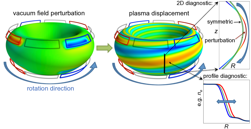
Figure 1: Cartoon of measuring the plasma displacement using a rigid rotating external MP-field. (left) external ’saddle’ coils produce a MP of the vacuum field. (middle) this MP-field causes a perturbation of the flux surfaces (only LCFS is shown). The color scaling of the surface plots indicates the magnetic perturbation $B_{r}$ (left) and the surface perturbation $\xi_{r}$ (middle) into direction normal to the LCFS. Red indicates a perturbation pointing outwards, blue inwards and green none. A rotation of the external MP-field (left) results in a rotation of the displacement (middle), which can be measured by an imaging system (right, top) or profile diagnostics (right, bottom). The rotation direction of the rigid rotation (in positive toroidal angle $\phi$) is indicated by blue arrows.

The measurement principle is based on external saddle coils, which produce non-axisymmetric MPs of the vacuum field. The result is a nearly pitch-aligned non-axisymmetric distortion of the flux surfaces, which is static to the MP-field. The main idea is that a rotation of this external MP-field leads to a rotation of the displacement (illustrated in Figure 1). This rotating distortion is then measured by profile and/or imaging diagnostics [18]. The rotating distortion should appear in profile diagnostics as radially varying displacement. Their high spatial resolution can be used to accurately measure the amplitude of the distortion [28, 29]. From the imaging diagnostics, we can gain information about the alignment of the distortion by inspecting the poloidal phase of the plasma response as a function of the continually varied toroidal phase of the external MP-field. The present experiment was made with the toroidal magnetic field and plasma current pointing in opposite directions, hence negative safety factor q. Consequently, an imaging system should detect a poloidally downward propagating structure, if the rotation is in positive toroidal direction (counterclockwise in the cartoon). The rotation directions are indicated by blue arrows in Fig. 1.

In this paper, we focus on ECE diagnostics for profile and imaging measurements. They are ideal to track changes of the flux surfaces, since they are able to deliver the electron temperature ($T\rm{{}_{e}}$) with high temporal resolution. Due to the very large electron heat diffusivity along the magnetic field lines, $T\rm{{}_{e}}$ is essentially constant on flux surfaces.

2.1 MP-coils and edge diagnostics

ASDEX Upgrade is equipped with 16 MP-coils, which are arranged in two poloidally separated rows and each has eight toroidally equidistant coils [30] (shown in Fig. 1). This allows us to apply an MP-field with a toroidal mode number $n$ of 1, 2 and 4. A newly installed power supply system enables us to rotate the MP-field of the two coil sets separately [31]. Thus, it is possible to employ either a differential rotation (sets in opposite direction) or a rigid rotation (both sets in same direction) using $n=1,2$ with frequencies up to several $100\ \rm{Hz}$ [31]. Because of the passive stabilization loop (PSL) conductors in ASDEX Upgrade, fast rotating MP-fields are attenuated and delayed by image currents [32]. To avoid significant attenuation, we applied a low frequency of $0.5\ \rm{Hz}$ for the $n=2$ rigid rotation [33]. The estimated attenuation is not more than $10\%$. We used even parity configuration for the rigid rotation, which means that the differential phase angle between the MP-field of the upper and lower coil set $\Delta\phi\rm{{}_{ul}}$ is $0^{\circ}$ [34]. Since there are 8 saddle coils in each row, the toroidal mode spectrum of the external MP-field exhibits a dominant $n=2$ and weak $n=6,10,14,\dots$ components but no other additional side bands. The intrinsic error field for $n=2$ is assumed to be small, because: First, no global density perturbation have been observed during the $n=2$ rigid rotation and second, dedicated measurements of the $n=1$ error field also indicates only a small $n=2$ component (no ellipse in Fig. 4 in Ref. [35]).

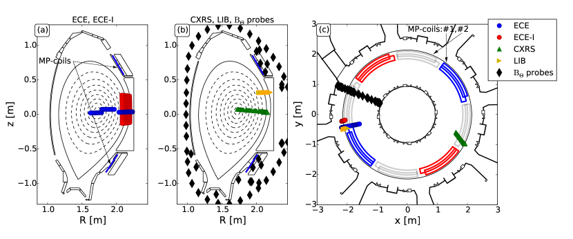
Figure 2: Overview of the used diagnostics and the MP-coils. (a) and (b) are poloidal cross-section showing ECE, ECE-I and CXRS, LIB, $B_{\Theta}$ probes, respectively. (c) top view. Dotted arrows indicate the poloidal (a) and the toroidal position (c) of the MP-coils. The coil numeration of each coil-set is shown in (c). The colors of the MP-coils illustrates an $n=2$ perturbation.

To obtain the edge displacement accurately, several high resolution edge diagnostics are in use. Figure 2 shows the poloidal (Fig. 2(a),(b)) and toroidal (Fig. 2(b)) positions of CXRS [36], LIB [37, 38], ECE and ECE-I, which measure ion temperature ($T\rm{{}_{i}}$), electron density ($n\rm{{}_{e}}$) and $T\rm{{}_{e}}$, respectively. Additionally, the magnetic probes used for the equilibrium reconstruction and plasma position control are shown.

As mentioned previously, we mainly use ECE measurements to track 3D distortions of the flux surfaces. To obtain reliable edge profiles of $T\rm{{}_{e}}$ from ECE, it is necessary to forward model the electron cyclotron radiation transport [26]. The 1D-profile ECE diagnostic (blue circles in Fig. 2) uses a heterodyne radiometer with 60 channels and a sampling rate of $1\ \rm{MHz}$ to measure the second harmonic extraordinary mode (X2). At the standard magnetic toroidal field configuration of $B\rm{{}_{T}}\approx-2.5\ \rm{T}$, 36 channels cover the edge region with a spatial resolution of about $5\ \rm{mm}$. This spatial resolution is set by the frequency spacing between the channels, the intermediate frequency (IF) bandwidth of $300\ \rm{MHz}$ of each channel and the additional broadening due to electron cyclotron radiation transport effects like Doppler broadening. The remaining 24 channels are used to measure the core using a frequency spacing of $\approx 1\ \rm{GHz}$ and an IF bandwidth ($f\rm{{}_{IF}}$) $600\ \rm{MHz}$ resulting in a spatial resolution of about $12\ \rm{mm}$. The 1D-profile ECE system is calibrated absolutely [39, 40], whereas the ECE-I system relies on a cross calibration.

The used ECE-I system has 128 channels (red circles in Fig. 2) with a temporal resolution of $200\ \rm{kHz}$ [41]. It was configured to cover the plasma edge using X2. It has 16 rows with a vertical spacing of $\approx 25\ \rm{mm}$ and 8 channels in each row. The frequency spacing is $800\ \rm{MHz}$, whereas $f\rm{{}_{IF}}$ is $700\ \rm{MHz}$. The resulting radial spatial resolution is around $15\ \rm{mm}$ at the edge. The advantage of ECE-I is that the vertical distribution of the channels allows us to resolve poloidal structures. Because of a recent extension to a quasi 3D system [42], the toroidal angle between the geometrical lines of sight (LOS) of the ECE-I system and the toroidal field is oblique. This complicates the interpretation of the ECE-I system and it is necessary to forward model the ECE-I. This is treated in detail in section 3.

Measuring the 3D displacement using toroidally localized diagnostics and a rigid rotating MP-field is based on two assumptions: First, the measured plasma parameters are constant on the perturbed flux surfaces and second, global plasma parameters, like core temperature and density, do not change significantly during the rigid rotation. The validity of both assumptions is justified in the following section.

2.2 Discharge

The presented experiment at ASDEX Upgrade was done at a plasma current of $I_{P}=800\ \rm{kA}$ and a toroidal field of $B\rm{{}_{T}}=-2.5\ \rm{T}$ (direction of $B\rm{{}_{T}}$ is clockwise). In this configuration, the direction of the ion $\nabla B$ drift is towards the X-point and the edge safety factor amounts to $q\rm{{}_{95}}\approx-5.4$. Figure 3 shows the time traces of global plasma parameters during the application of the MP-coils. The rotation was performed with a frequency of $0.5\;\rm{Hz}$ indicated by the MP-coil currents in Fig. 3(a). Two periods in positive toroidal direction were performed and in-between the neutral beam injection (NBI) power was stepped from $5$ to $7.5~{}\rm{MW}$. Within one NBI step, the density and temperature do not vary more than $6\%$ in the core (Fig. 3(c,d)). The normalized beta $\beta_{N}$ amounts to $\approx 1.7$ and $\approx 2$ in the second NBI power step (see Fig. 3(e)). The application of this MP-coil configuration does not significantly affect the ELM behavior as seen in the divertor current (Fig. 3(f)). ELM mitigation is also not expected for these plasma parameters with an even parity configuration ($\Delta\phi\rm{{}_{ul}}\approx 0^{\circ}$). The optimum phase angle for ELM mitigation for this ’high $B\rm{{}_{T}}$’ and ’high $q$’ case scenario is, according to MARS-F [12] calculations, $\Delta\phi\rm{{}_{ul}}\approx-90^{\circ}$ (Fig. 11 in Ref. [20]).

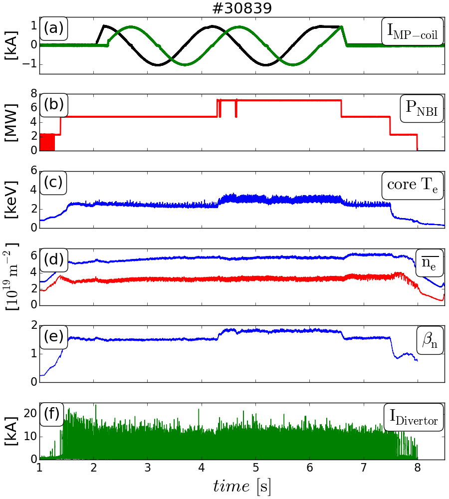
Figure 3: Discharge overview: (a) coil current of the first (black) and second (green) MP-coil from the upper coil-set (see Fig. 2(c)) to indicate the time period of the rigid rotation, (b) heating power, (c) core electron temperature, (d) line integrated density from a core (blue) and an edge chord (red), (e) normalized beta $\beta_{N}$ and (f) divertor current. The rigid rotation does not alter global plasma parameters.

It is clearly seen in Figure 3 that core densities and temperatures do not change significantly during the rigid rotation (less than $6\%$). This confirms the assumption of constant global plasma parameters. The time traces of Figure 3 also suggests that the first assumption of constant measured plasma parameters on perturbed flux surfaces in the pedestal region is fulfilled. The breaking up of flux surfaces due to stochastization in the bulk of the pedestal would result in a significant decrease of the temperature and density gradients in the pedestal and, consequently, also of the core temperature and density. Since there is no pronounced drop of these parameters during the switching on of the MP-field, a stochastization of the entire gradient region can be ruled out. Strike point splitting [43] is observed, which indicates a break in axisymmetry. But there is no hint for stochastization within the edge region. Moreover, we can also assume that ideal MHD is applicable in this case, which is discussed in section 4.3.

2.3 Edge measurements during rigid rotation

Although core $n\rm{{}_{e}}$, $T\rm{{}_{e}}$ and $T\rm{{}_{i}}$ values are almost constant in time, every edge profile diagnostic observes a radial position shift due to the rigid rotation of the MP-field. Time traces from ECE, ECE-I, LIB and edge CXRS in Fig. 4 show a clear modulation due to the radial shift. To visualize the modulation, we only use data from pre-ELM time points ($50-80\%$ of the ELM cycle). Figure 4(b) illustrates ECE measurements using all time points (red) and using pre-ELM time points only (blue).

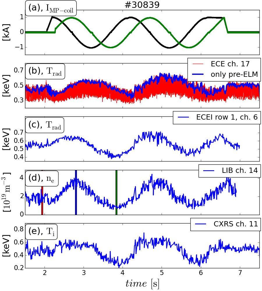
Figure 4: Edge measurements during the rigid rotation: (a) same coil currents as in Fig. 3(a) to indicate the rigid rotation, (b) time traces of one edge ECE channel using all time points (red) and using pre-ELM time points only (blue). Panel (c), (d) and (e) show time traces from one ECE-I channel, LIB and edge CXRS, respectively, using pre-ELM time points only. Vertical bars in (d) indicate the time windows used in Fig. 5. The edge perturbation is seen in each edge diagnostic.

To demonstrate that the MP-field perturbs the entire edge profile, Fig. 5 shows edge $n\rm{{}_{e}}$ profiles from LIB before the MP onset (Fig. 5(a) red), at the maximum displacement (Fig. 5(b) blue) as well as at the minimum displacement (Fig. 5(b) green). To account for additional small plasma movement within the analyzed time windows of $40\ \rm{ms}$, the profiles are plotted against $R$ relative to the separatrix position determined from the routinely used axisymmetric equilibrium reconstruction (temporal resolution is $1\ \rm{ms}$) [44]. The steep gradient region is well determined by the LIB diagnostics, whereas the pedestal top measurements exhibit relatively large uncertainties (see Fig. 5(a)) and, hence, large scatter. This is because of a decreasing sensitivity of the LIB diagnostics towards the plasma core [38]. However, the edge $n\rm{{}_{e}}$ profiles between the maximum and the minimum displacement show a clear change in the real space gradients, whereas pedestal top values remain, within their uncertainties, the same. This indicates that the MP-field induces flux surface expansions and compressions, which depends on the toroidal phase.

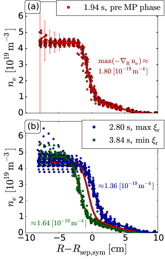
Figure 5: $\#30839$, edge $n\rm{{}_{e}}$ profiles from the LIB diagnostic versus $R$ relative to the axisymmetric separatrix using only pre-ELM time points: (a) profiles before the MP-onset (red). The measurement uncertainties from one time point are indicated by error-bars in (a). The maximum density gradient in real space (text inset) are determined from the spline (solid line). (b) same for profiles at the maximum (blue) and minimum (green) displacement $\xi_{r}$. For comparison, the fit (red line) from (a) is shown. The analyzed time windows are indicated by vertical bars in Fig. 4. The gradients are changing during the rotation suggesting a flux surface expansion and compression.

In addition to the toroidal symmetry breaking, the MP-field also adds poloidal structures. This is expected from various plasma response calculations [45] and is observed by the ECE-I system. Figure 6(a) shows the mean radiation temperature during the rigid rotation using the cold resonance positions for the mapping (details about cold resonance position in Section 3). The solid line indicates the LCFS and the dashed line a flux surface within the pedestal region at a normalized poloidal flux of $\rho\rm{{}_{pol}}\approx 0.972$ (the used definition of $\rho\rm{{}_{pol}}$ is in Ref. [46]). Time traces using only pre-ELM time points of channels along this flux surface and a least square (LSQ) fit of a sine function including their higher harmonics are shown in Figure 6(b). The modulation is observed in each of these channels. Furthermore, this modulation is propagating downwards as expected from a MP-field rotation in positive toroidal direction (see Fig. 1 for illustration).

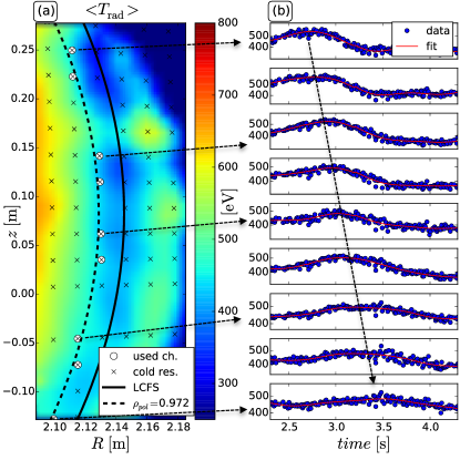
Figure 6: (a) The color code shows the mean of radiation temperature $<T\rm{{}_{rad}}>$ throughout the rigid rotation ($t\approx 2.2-4.4\;\rm{s}$) measured by the ECE-I. Crosses mark the channel positions. Circles indicate channels close to a flux surface in the pedestal $\rho_{pol}\approx 0.972$. The lines indicate a flux surface in the pedestal $\rho_{pol}\approx 0.972$ (dashed) and the last closed flux surface (solid). (b) Time traces of $T\rm{{}_{rad}}$ and their corresponding LSQ fit from channels marked as circles in (a). The modulation is propagating downwards.

ECE-I measurements during the rigid rotation contain valuable information about the flux surface displacement. The perturbation is usually characterized using the Fourier decomposition of its normal component $\xi\rm{{}_{r}}=\xi_{a}\ e^{i(m\Theta^{\star}-n\phi)}$, where $\xi_{a}$ is the amplitude, $n$ the toroidal mode number, $\phi$ the toroidal angle, $m$ the poloidal mode number and $\Theta^{\star}$ the straight field line (SFL) angle [47] (see Section 4.2). $\xi\rm{{}_{r}}$ directly measures the displacement between the axisymmetric and 3D equilibrium [14]. Because of its poloidally and radially localized channels, the ECE-I diagnostic is able to resolve the poloidal mode numbers $m$. One can obtain $m$ using $m=\frac{\Delta\phi}{\Delta\Theta^{\star}}$, where $\Delta\phi$ and $\Delta\Theta^{\star}$ are the toroidal phase increment and the corresponding SFL angle difference between the various ECE-I channels. Therefore, the determination of $m$ depends strongly on the accuracy of the calculated SFL angle. Because of the high shear in the pedestal region, the calculation of $\Theta^{\star}$ is very sensitive to the used flux surface. The correct positions and the corresponding flux surfaces of the ECE-I channels are therefore essential to determine the poloidal mode structure accurately. To provide accurate measurement positions of the ECE-I channels, we applied forward modeling of the radiation transport, which is described in the next section.

3 Interpretation of ECE

The ECE-I diagnostic was extended to allow quasi-3D measurements using a second ECE-I system, which was not in use at the time of this experiment [42]. To enable these quasi-3D measurements, it was necessary to change the LOS geometry (see Ref. [42]). This increased the toroidal inclination angle $\angle$ between the LOS and the normal to the flux surface or rather the magnetic field line. Therefore, the LOS are oblique and not perpendicular anymore, which enhances the Doppler-shift of the observed ECE intensities. As a consequence, the position where the measured frequency fulfills the electron cyclotron resonance condition (cold resonance position) [48] is not a good approximation for the measurement position or rather the position of the observed ECE intensity. The reason for this is that the cold resonance position does not account for kinetic effects like the relativistic mass increase and the Doppler-shift [40]. This section describes the determination of the distribution of the observed ECE intensity and its maximum is labelled as ’warm’ resonance position (’warm’ because kinetic effects are also included, see also Ref. [49, 50]). The analysis in this section is done for a time-point prior to the MP onset, hence, axisymmetry is assumed.

3.1 Definition of the ’warm’ resonance position

$T\rm{{}_{e}}$ is routinely determined from the radiation temperature ($T\rm{{}_{rad}}$) of the 1D ECE measurements using a forward model within the framework of the integrated data analysis (IDA) [26, 51]. The $T\rm{{}_{e}}$ profile is varied until the most likely match between the measured and estimated ECE intensity within the Bayesian analysis is found. The ECE intensity is calculated by solving the radiation transport equation along the LOS [26] of the ECE diagnostic for given $T\rm{{}_{e}}$ and $n\rm{{}_{e}}$ profiles. Because we are mainly interested in the origin of the observed intensity, we only use the module of IDA, which solves the radiation transport equation (details in Ref. [26]). For this purpose, $T_{e}$ and $n_{e}$ profiles from routine IDA evaluation serve as input [46].

To account for additional refraction, we extend the modeling by ray tracing (details in Ref. [51]), which is found to be in good agreement with the TORBEAM code [52]. The ray tracing code calculates the ray path of each channel until the ray hits the wall. Then, the radiation transport equation is solved along the ray path starting from the end of the ray towards the diagnostic antenna. The combination of forward modeling and ray tracing allows us to determine exactly the origin of the observed intensity. The distribution of the observed intensity ($D_{\omega}$) [51] is the normalized product of the emissivity $j_{w}(s)$ and the transmittance $T_{\omega}(s)$ along the ray path coordinate $s$:

$$D_{\omega}(s)=\frac{j_{w}(s)\ T_{\omega}(s)}{\int j_{w}(s)\ T_{\omega}(s)ds}$$ (1)

Figure 7(a) and (b) illustrate $j_{w}$, $T_{\omega}$ [51] and the resulting $D_{\omega}$, respectively, versus $\rho_{pol}$ calculated for one 1D-ECE channel in the pedestal region. The used $T\rm{{}_{e}}$ profile and the modeled $T\rm{{}_{rad}}$ ($T_{\rm{rad,mod}}$) value of this channel at its cold resonance position are also shown. Although we neglect the IF bandwidth, the calculated $D_{\omega}$ is relatively broad, which is attributed to the Doppler and the relativistic broadening.

To have a single quantity as an approximation for the measurement position of a single ECE channel, we use the maximum of $D_{\omega}$ labelled as ’warm’ resonance position [53] (shown in Fig. 7). As indicated by the vertical lines in Fig. 7(b), the ’warm’ resonance position can differ from the cold resonance position. This discrepancy originates from the Doppler effect due to an oblique LOS of $\angle\approx 8.6^{\circ}$. Although the toroidal inclination angle of the profile ECE system amounts to only $\approx 4^{\circ}$ and almost no poloidal inclination angle, additional refraction by the plasma leads to an even larger angle at the cold resonance position. As a result, the Doppler-shift becomes more important, especially, in the case of the ECE-I system.

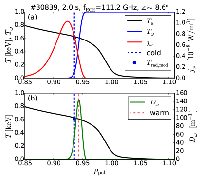
Figure 7: $\#30839$ at $2.0\ \rm{s}$, (a) emissivity $j_{\omega}$ and the transmittance $T_{\omega}$ are shown along the ray path mapped on $\rho\rm{{}_{pol}}$. (b) The resulting distribution of the observed intensity ($D_{\omega}$) and its maximum, the ’warm’ resonance position is indicated by a vertical dotted line. In both frames, the used $T_{e}$ profile (solid, black) and the cold resonance position (vertical dashed) are shown.

3.2 ’warm’ resonance position of ECE-I channels

Because of a toroidal inclination angle at launch of $\angle\approx 7.2^{\circ}$ and additional poloidal angles, the Doppler-shift influences the ECE-I even more in the case of the profile ECE system. Figure 8(a) and (b) show a comparison between the $D_{\omega}$ of one 1D-ECE channel and one from the ECE-I system at similar $(R,z)$ cold resonance positions. For the shown ECE-I channel, refraction causes an angle of $\approx 17.7^{\circ}$. This leads to a significant broader $D_{\omega}$ and to an even larger shift between the cold and ’warm’ resonance position ($\approx 15\ \rm{mm}$).

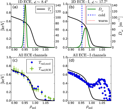
Figure 8: Discharge $\#30839$ at $2.0\ \rm{s}$, (a) $D_{\omega}$ from an 1D-ECE channel at the pedestal top is shown. Cold and ’warm’ resonances are indicated by vertical dashed and dotted lines, respectively. The modeled $T\rm{{}_{rad}}$ ($T_{\rm{rad,mod}}$) is shown at its cold resonance position as blue circle. (b) same as (a) for an ECE-I channel at similar position. (c) modeled (circle) and measured $T\rm{{}_{rad}}$ ($T_{\rm{rad,ECE}}$, diamonds) at their cold resonance position from all edge ECE channels. (d) modeled $T\rm{{}_{rad}}$ for the ECE-I channels. The used $T\rm{{}_{e}}$ profile is plotted in all frames as a reference.

Figures 8(c) and (d) present the modeled radiation temperature ($T_{\rm{rad,mod}}$) at their cold resonance position from all profile ECE and ECE-I channels covering the edge, respectively. Additionally, Fig. 8(c) also shows the absolutely calibrated ECE measurements (yellowgreen diamonds). The measured and modeled $T\rm{{}_{rad}}$ are in good agreement, which underlines the correct description of these measurements. In the far scrape off layer (SOL) ($\rho\rm{{}_{pol}}>1.05$), the measurements deviate from the model. These channels have a very low optical depth ($\tau_{\omega}<1$) [48] so that wall reflections are becoming important [51]. But for channels having an optical depths typical for the pedestal region ($\tau_{\omega}>5$) or more, wall reflections contribute less than one per mill to the measured $T\rm{{}_{rad}}$ [26]. Since we are mainly interested in $T\rm{{}_{rad}}$ values from the pedestal region, wall reflections are not taken into account.

The well-known ’shine-through’ peak appears in both systems [54] and it is even more pronounced in the ECE-I system due to their oblique LOS. Furthermore, $T\rm{{}_{rad}}$ values differ from $T\rm{{}_{e}}$ not only in the optically thin region ($\tau_{\omega}<5$ for $\rho\rm{{}_{pol}}>1.0$) but also in the optically thick region ($\tau_{\omega}>5$). This is more obvious for the ECE-I system and shows that the classical ECE approach [26] is also not applicable to ECE-I channels in the optically thick region. To avoid misinterpretation of the ECE-I measurements, it is therefore required to perform the forward modeling for all channels.

Especially, the implementation of the ray tracing is important to determine accurate ($R,z$) values for the ’warm’ resonance position. This is illustrated in Fig. 9, which shows ($R,z$) of the ’warm’ and the cold resonances. Remarkably, the majority of the ECE-I channels in this configuration probe the pedestal region. The channels in the optically thick region measure electrons located in this region due to the Doppler-shift, whereas the SOL channels observe only the down-shifted radiation of the Maxwellian tail [26]. One should keep in mind that the Doppler-shifted observation in the optically thick region is a feature due to the oblique LOS, whereas the feature of the SOL channels probing the pedestal region appears also for the case of perpendicular ECE views (see Ref. [54]). Since the SOL channels also contain valuable information, we will also include them in our analysis.

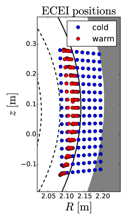
Figure 9: $\#30839$ at $2.0\ \rm{s}$. Cold and ’warm’ resonance positions of all ECE-I channels. Differences in $R$ and $z$ between cold and ’warm’ resonances are apparent.

In the following, we will use the ’warm’ resonance positions as measurement positions and assume that they are constant during the rigid rotation. In principle, there are two possibilities which can modify the measurement position during the rigid rotation: First, a change in the total magnetic field due the MP-field could change the cold resonance position and hence, the ’warm’ resonance position as well. The relative strength of the external MP-field in front of the MP-coils is $|\delta B|/|B|<10^{-3}$ and around the midplane, it is even lower $|\delta B|/|B|<10^{-4}$. The resulting difference in the resonant position using the latter case is $\delta R<0.2\ \rm{mm}$ at $R\approx 2\ \rm{m}$. Thus, we assume that the resonance position is constant during the rigid rotations. Second, refraction due to a 3D geometry can additionally deflect the LOS ray and vary the measurement position. At the moment, the forward model of the ECE and the underlying ray tracing are not capable to deal with 3D flux surfaces. But, this additional toroidal angle is expected to be small, since $\delta\phi<\rm{arctan}(|\delta B|/|B|)=\rm{arctan}(10^{-4})\approx 0.006^{\circ}$. Even a relatively strong $n=2$ radial flux surface displacement $\xi_{r}$ of $2\;\rm{cm}$ at $R\approx 2\ \rm{m}$ would result in an additional toroidal angle of only $\delta\phi<\rm{arctan}(n\ \xi_{r}/R)\approx 1.1^{\circ}$. Because of these small additional angles, they impact on the modeling of the electron cyclotron radiation transport is small, which justifies the neglect of additional refraction due to toroidal asymmetry on the ray tracing.

The combination of the forward modeling and ray tracing allows us to determine accurate ($R,z$) values of the ’warm’ resonance position for the ECE and ECE-I diagnostics. These positions are used to calculate the SFL angle and are, therefore, essential for its interpretation. Of course, this approach is only valid if the $D_{\omega}$ is not bimodal and has only one dominant peak. This is the case for the ECE and in the majority of the ECE-I channels. Moreover, the forward modeling enables us to compare $T\rm{{}_{rad}}$ from the ECE measurements with calculated synthetic $T\rm{{}_{rad}}$ using the 3D equilibrium from VMEC. The generation of the synthetic data from VMEC will be elucidated in the following section.

4 Synthetic data from ideal MHD equilibrium (VMEC)

To compare measurements with an ideal MHD equilibrium, we use the free boundary version of VMEC [27]. VMEC uses a variational principle to determine the shape of a set of nested flux surfaces [55]. In the free boundary version, the external MP-field enters the calculations by the boundary condition. The plasma energy ($W\rm{{}_{MHD}}$) is then self-consistently minimized while the plasma boundary is varied to make the total pressure $\frac{1}{2\mu_{0}}B^{2}+p=\frac{1}{2\mu_{0}}B^{2}_{V}$ continuous at the plasma boundary. The normal component of the vacuum field $\vec{B}_{V}$ vanishes such as $\vec{B}_{V}\cdot\vec{n}_{p}=0$ ( $\vec{n}_{p}$ = normal vector at the plasma boundary). The vacuum field $\vec{B}_{V}$ is produced by all external conductors (e.g. toroidal field coils, shaping and perturbations coils). The converged 3D equilibrium is a nonlinear solution of the ideal MHD model. This implies that (a) non-linear coupling of toroidal modes is correctly represented and (b) the solution preserves inherently the original topology with nested flux surfaces, i.e. magnetic islands cannot be described. This latter property corresponds to perfect shielding of resonant field components. In contrast to other formulations, the variational method ensures this intrinsically, without the need to adjust surface currents at rational flux surfaces as done e.g. in perturbative codes.

4.1 Equilibrium inputs

The axisymmetric equilibrium reconstruction CLISTE from discharge $\#30839$ at $t=3.2\ \rm{s}$ serves as an input [44]. To reduce the influence of the MP-coils on the reconstruction, we choose a time point, when the MP-coils located closely to the $B_{\Theta}$ probes have almost zero current. This is demonstrated in Fig. 2(c), where the color scaling indicates the coil current at $t=3.2\ s$ and the $B_{\Theta}$ probes are shown as well.

The pressure $p$, toroidal current and the safety factor $q$ profile (Fig. 10) in the CLISTE equilibrium are restricted by kinetic profiles, a self-consistent bootstrap current in the edge gradient region and a prescribed minimum $q$ above 1 to avoid an unstable helical plasma core in VMEC, respectively. For the pressure constraints, the pressure profile was determined at $t=3.2\ \rm{s}$ using various profile diagnostics like LIB, CXRS, Thomson scattering (TS), etc. The contribution from the fast particles is not taken into account, but this is usually negligible in the pedestal [56]. Because of the steep density and temperature profiles in the pedestal, the resulting bootstrap current causes a flattening in the $q$ profile (around $\rho_{pol}\approx 0.97$, $q\approx 5.4$ in Fig. 10). Since VMEC only deals with nested flux surfaces, the SOL is not considered and SOL currents were excluded in the reconstruction of the input equilibrium. Moreover, the flux surfaces were truncated at $\rho\rm{{}_{pol}}\approx 0.9999$ to avoid the singularity of the X-point. One should also keep in mind that the axisymmetric solution of the converged VMEC equilibrium can slightly vary from the CLISTE equilibrium. But this difference is small and can be balanced by shifting the plasma vertically and/or radially a few millimeters ($3-4\ \rm{mm}$). More details about the implementation of the VMEC code at ASDEX Upgrade is described in Ref. [14]. MARS-F calculations are also employed to supplement the comparison and the inputs are the same as for VMEC.

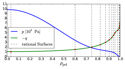
Figure 10: Total pressure $p$ and the safety factor $q$ are shown. Vertical lines indicate the rational surface positions for $n=2$.

4.2 Calculation of straight field line coordinates and poloidal mode spectra

The calculations of the poloidal mode spectra and the comparison to the ECE-I measurements require the usage of SFL coordinates ($\theta^{\star}$, $\phi^{\star}$). On the flux surface $\rho$, they are defined such that $d\phi^{\star}/d\theta^{\star}=q(\rho)=const$. In this paper, we primarily use SFL coordinates (PEST-like [57]), where the Jacobian for the coordinate transformation with the cylindrical coordinates is proportional to $R^{2}$. Moreover, the toroidal angle is the geometrical angle $\phi^{\star}=\phi$ and, thus, only the poloidal SFL angle $\theta^{\star}$ has to be determined. For more details, we refer the readers to Chapter $6.2$ in Ref. [47] or Chapter 2.2.1.4 in Ref.  [58]. As an exception and due to historical reasons, the poloidal mode spectra of the VMEC output are calculated using Boozer coordinates [59]. But this makes almost no difference for the analysis since only the axisymmetric equilibrium, as in all cases, is used to calculate the SFL coordinates and hence, the poloidal mode spectra.

To verify the calculations of the SFL coordinates and the mode spectra, Fig. 11 shows the $n=-2$ poloidal mode spectra of the external MP-field in the vacuum field approximation using the axisymmetric equilibrium from CLISTE (Fig. 11(a)), VMEC (Fig. 11(b)) and MARS-F (Fig. 11(c)). The color scaling indicates the amplitude of the perturbed magnetic field component which is normal to the unperturbed flux surface $B\rm{{}_{r}}$. To account for the components with the same helicity of the Fourier spectrum ($n=+2$), the illustrated $n=-2$ amplitudes are multiplied by a factor of 2. Since ASDEX Upgrade has negative $q$ in this case, only positive poloidal mode numbers are relevant for the negative toroidal mode components. This is also seen by the components (dashed line), which have the same helicity as the equilibrium field-line pitch (pitch aligned) and the resonant (circle) components in Fig. 11(a-c). In general, the poloidal mode spectra are in good agreement, which gives confidence about the representation of the external MP-field. The mode spectra of one flux surface at the edge ($q=-5$) are illustrated in Fig. 11(d). Slight deviations are mainly because of small differences in the axisymmetric equilibria (mm variation in position and shape) and the MP-coil current representation (e.g. MARS-F uses Fourier representation [15]). The analyzed coil configuration is even parity with $|n|=2$ and for the present plasma configuration with $q_{95}=-5.4$, the external MP-field is almost non-resonant (Fig. 11(d)). The grey bar in Fig. 11(d) indicates the resonant field component.

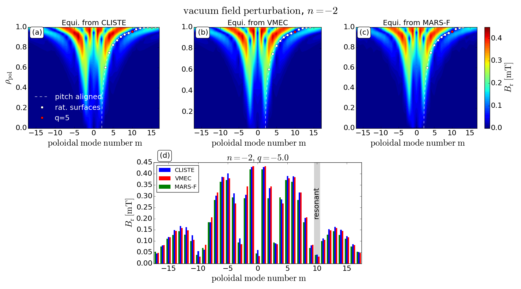
Figure 11: The poloidal mode spectra of the external MP-field $n=-2$ in the vacuum field approximation, $\rho_{pol}$ versus poloidal mode number $m$ using (a) CLISTE equilibrium of $\#30839$ at $3.2\ \rm{s}$, $n=0$ solution of (b) VMEC and (c) MARS-F. Color scaling indicates the strength of the radial field perturbation $B\rm{{}_{r}}$. The pitch aligned components and the rational surfaces are shown as dashed line and white circles, respectively. (d) poloidal mode spectra of $q\approx-5.0$ ($\rho_{pol}\approx 0.955$) surface indicated as red circle in (a-c). Its resonant component is illustrated by a grey bar. The external MP-field is almost non-resonant.

4.3 Justification of using ideal MHD

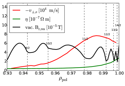
Figure 12: Perpendicular electron velocity $v_{\perp}$, Spitzer resistivity $\eta$ and pitch aligned radial component of the vacuum field perturbation $B\rm{{}_{r,res}}$ are shown. Usually high $v_{\perp}$, low $\eta$ and, for this case, low $B\rm{{}_{r,res}}$ are observed in the pedestal.

Since VMEC is an ideal MHD code with nested flux surfaces, no resistive MHD effects are included and no magnetic island can appear. The appearance of magnetic islands at the rational surfaces depends on the plasma resistivity $\eta$ as well as on the velocity of the plasma frame expressed by the perpendicular electron velocity $v_{\perp,e}$ and the field strength of the resonant component of the external MP-field normal to the unperturbed flux surface $B\rm{{}_{r,res}}$. The velocity of the plasma frame in the pedestal is relatively high $v_{\perp,e}(q=-5.5)\approx-60\ \rm{km/s}$ (Fig. 12) due to the dominant diamagnetic velocity [60]. Hence, it is expected that the, anyway small, pitch aligned components from the external MP-field are screened. The resistivity in the pedestal region is low due to the high $T_{e}$. The calculated Spitzer resistivity is shown in Figure 12. Because of the low pitch aligned components, the high $v_{e,\perp}$ and low $\eta$, magnetic islands are unlikely in this case. In order to further justify our use of ideal MHD, we employed MARS-F calculations once with ideal MHD and once with resistive MHD using Spitzer resistivity ($\eta\rm{{}_{Spitzer}}$). The resulting magnetic perturbation of the plasma response field between ideal and (Spitzer) resistive MHD differ only by maximal $0.01\ \rm{mT}$ in the poloidal mode spectra (not shown). This also implies that the resonant components of the plasma response field are also smaller than $0.01\ \rm{mT}$. In comparison to the values from the vacuum field calculations (see Fig. 11), this difference is very small. Moreover, the displacement of the resistive MHD calculations exhibits no phase flip. This underlines the use of ideal MHD.

4.4 The VMEC calculation

To have sufficient accuracy of the resulting equilibrium, we used 1000 flux surfaces, 17 toroidal mode numbers ($n=-8,\dots,8$) and 25 poloidal mode numbers for one period. Because of $n=2$, only one toroidal half was calculated. The toroidal ripple was not considered. The properties of the resulting 3D VMEC equilibrium are shown in Fig. 13. The radial displacement $\xi\rm{{}_{r}}$ is almost pitch aligned and strongest at the edge (Fig. 13(a) and details of the edge in Fig. 19(c)). The poloidal mode spectra can also be seen from a poloidal cut $\phi=0^{\circ}$ of $\xi\rm{{}_{r}}$ (Fig. 13(b)). The amplitude of the $n=-2$ displacement along the toroidal coordinate is shown in Fig. 13(c). It is pronounced around the midplane at the LFS (Fig. 13(b)).

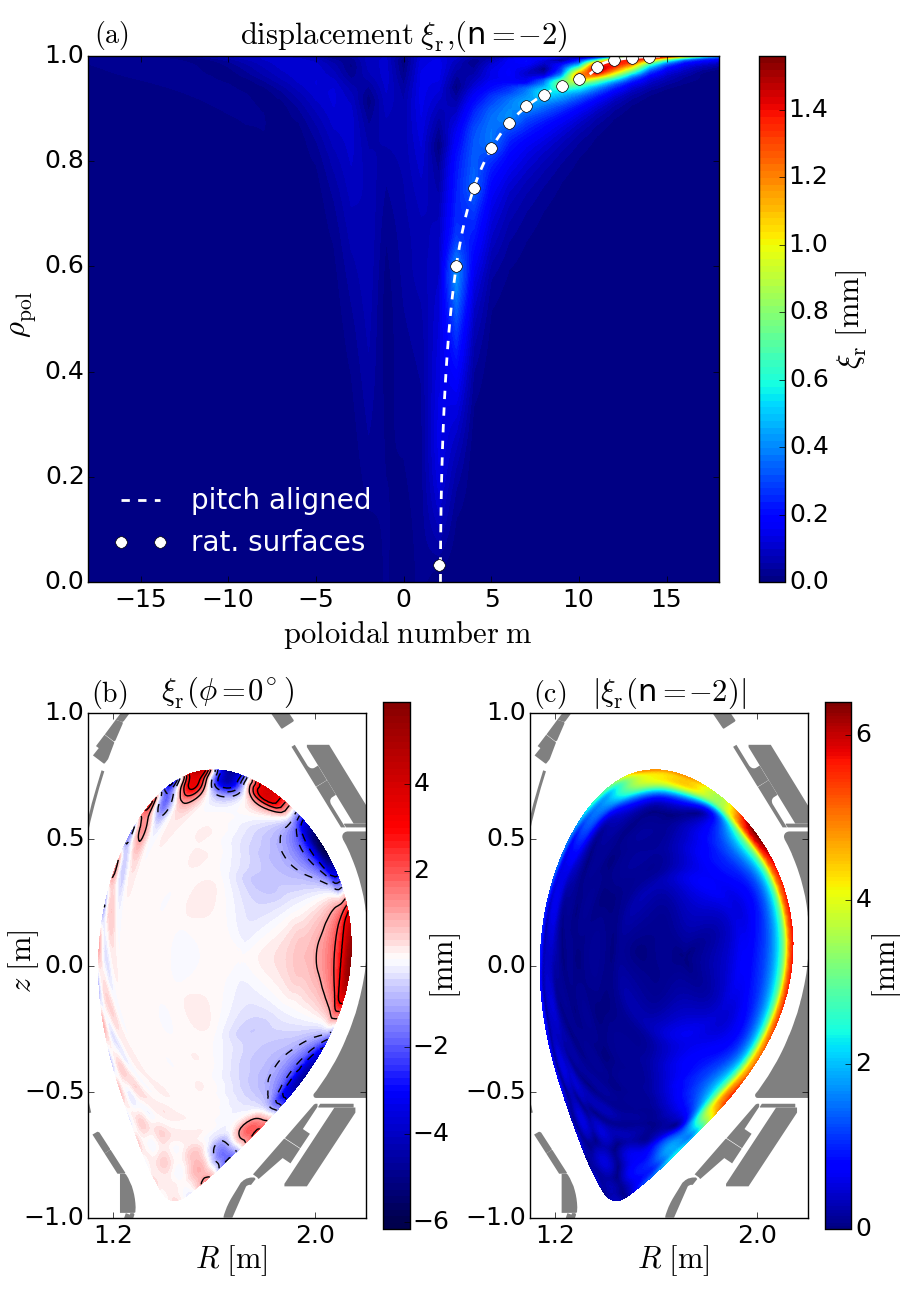
Figure 13: Radial displacement $\xi_{r}$ from VMEC, (a) $\rho_{pol}$ versus the poloidal mode spectrum $m$ of the $n=-2$ component of $\xi_{r}$ amplitude, (b) poloidal cut of $\xi_{r}$ at a toroidal angle of $0^{\circ}$ and (c) poloidal distribution of the $n=-2$ displacement amplitude along the toroidal coordinate. A kink response with $m\sim 9-15$ at the edge ($\rho_{pol}>0.9$) around the LFS midplane is apparent.

The VMEC calculations also exhibit a small $n=4$ component, which can solely be attributed to the plasma response (not shown). The explanation is as follows: ASDEX Upgrade has 8 saddle coils in each row. Hence, the $n=2$ perturbation can be described as a rectangular function along the geometrical toroidal angle $\phi_{geo}$. The Fourier series of a rectangular function solely consists of odd harmonics ($1,3,5,\dots$). Consequently, the applied $n=2$ MP-field in the vacuum approximation has exclusively toroidal mode numbers of $n=2,6,10,\dots$. Additionally, the $n=6$ component is increased due to the aliasing effect from the $n=2$ perturbation using 8 saddle coils ($n\rm{{}_{aliasing}}=8-2$). However, ASDEX Upgrade has no $n=4$ component in the vacuum field spectra when applying an $n=2$ perturbation. In DIII-D, for example, this is not the case. It has 6 saddle coils in each row and the aliasing effect causes an $n=4$ component [61]. The combination of Ampere’s law $\vec{j}=\vec{\nabla}\times\vec{B}$ and the plasma equilibrium $\nabla\vec{p}=\vec{j}\times\vec{B}$ introduces a non-linear ($\approx B^{2}$) behavior due to the plasma response. This non-linearity can lead to the appearance of additional toroidal mode numbers like $n=4,8,12,\dots$. Therefore, a measured $n=4$ component would prove a plasma response. But according to VMEC the maximum displacement of $n=4$ amounts to $\xi_{r}(n=4)\approx 0.2\ \rm{mm}$ and is unlikely to be measured within the measurement accuracy.

4.5 Calculation of synthetic data

The output of VMEC is a 3D equilibrium calculated for one time point. To compare the toroidally localized measurements during a rigid rotation with this single 3D equilibrium, we developed synthetic diagnostics for the VMEC equilibrium. The most important steps to produce synthetic data are listed below:

• The currents of the MP-coils are used to map the timebase of the used diagnostic to the geometrical toroidal angle $\phi\rm{{}_{geo}}$ in VMEC or vice versa. It is mapped in such way that the calculated $\phi\rm{{}_{geo}}$ from the rotation corresponds to the toroidal position of the diagnostic at the time of the VMEC calculation ($t=3.2\ \rm{s}$). Each slice in $\phi\rm{{}_{geo}}$ can be correlated to a time point and vice-versa.

• Because of small discrepancies between the input equilibrium and the axisymmetric component of the VMEC solution, the entire VMEC equilibrium is shifted by $R=3\ \rm{mm},\ z=4.5\ \rm{mm}$ to align the surfaces at the LFS. This allows us to compare vacuum field calculations using the input equilibrium with VMEC at the LFS.

• The (R, z) positions of each channel are determined for each diagnostic and are assumed to be independent of time or rather $\phi\rm{{}_{geo}}$. In the case of ECE diagnostics, the ’warm’ resonance positions are used.

• $T_{e}$, $T_{i}$ and $n_{e}$ profiles before the MP onset are used to correlate the $\rho\rm{{}_{pol}}$ with $T_{e}$, $T_{i}$ and $n_{e}$ values assuming they are constant on the perturbed flux surface. Due to a slight increase in core $n_{e}$, the global $T_{e}$ slightly decreases. To account for this, we add a time or rather $\phi\rm{{}_{geo}}$ dependent scaling function. This function is a cubic spline and time traces from core channels were used to parametrize it.

• ($R_{i}$, $z_{i}$) of each channel $i$ and $\phi\rm{{}_{geo}}$ are used to deduce the corresponding $\rho\rm{{}_{pol}^{i}}(\phi\rm{{}_{geo}})$ values from the 3D VMEC equilibrium and therefore, also $T_{i}$ and $n_{e}$ values. To get synthetic $T\rm{{}_{rad}}$ values for ECE diagnostics, the electron cyclotron radiation transport is solved using the slices of the poloidal flux surface at the corresponding $\phi\rm{{}_{geo}}$ of the perturbed equilibrium. To solve radiation transport, $T_{e}$, $n_{e}$ profiles as in step (iv) are used and each slice in $\phi\rm{{}_{geo}}$ is assumed to be axisymmetric.

• The VMEC output has no SOL flux surfaces. To complete the synthetic profiles in the SOL, the CLISTE equilibrium is used for flux surfaces for $\rho\rm{{}_{pol}}>1.04$. To allow a smooth transition between the perturbed VMEC and the axisymmetric CLISTE equilibrium, we simply use a 2D cubic spline to interpolate in-between.

All these steps allow us to compare quantitatively synthetic data from VMEC with measurements from ECE-I, ECE, CXRS and LIB. Moreover, we distinguish between the comparison of the amplitude and phase or rather poloidal mode structure of the flux surface displacement. We deduce both by fitting the measured and synthetic data to sine function with its harmonics.

5 Amplitude comparison

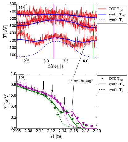
Figure 14: $\#30839$, (a) time traces of three channels using synthetic $T\rm{{}_{e}}$ (dashed blue), $T\rm{{}_{rad}}$ (solid blue), and the ECE data (solid red). Their radial positions are indicated by arrows in (b). (b) Synthetic $T\rm{{}_{e}}$ (dashed), $T\rm{{}_{rad}}$ (solid) and measured $T\rm{{}_{rad}}$ profiles (circles) at maximum (magenta) and minimum (green) displacement. The corresponding time points are indicated by the colored vertical bars in (a). Deviations between synthetic $T\rm{{}_{e}}$ and $T\rm{{}_{rad}}$ due to the ’shine-through’ effect are indicated. The synthetic and measured $T\rm{{}_{rad}}$ profiles are in good agreement.

In the following, we focus on the profile ECE system. Unlike the ECE-I, it has an absolute calibration and moreover, its spatial resolution is higher. Both is beneficial for the amplitude comparison. But like every ECE system, its interpretation at the plasma edge can be challenging due to the transition from the optically thick to the optically thin plasmas (also discussed in Ref. [23]). Because of the lack of density information at the ECE LOS in the presence of a 3D equilibrium perturbations, we are not able to accurately determine $T\rm{{}_{e}}$ profiles from ECE measurements. Therefore, we will primarily compare $T\rm{{}_{rad}}$ data instead of $T\rm{{}_{e}}$.

Figure 14 shows a comparison between ECE measurements, synthetic $T\rm{{}_{rad}}$ as well as synthetic $T\rm{{}_{e}}$ data. Both, the time traces (Fig. 14(a)) and the corresponding profiles (Fig. 14(b)) from the ECE and the synthetic $T\rm{{}_{rad}}$ diagnostic match very well. The boundary displacement is visible as a shift between between the profiles at the minimum and maximum displacement (magenta versus green in Fig. 14(b)). Moreover, the synthetic $T\rm{{}_{rad}}$ profiles correctly describe features of the ’shine-through’ peak. For example, the gradients of the edge $T\rm{{}_{e}}$ profile are smaller at the maximum displacement (magenta profiles in Fig. 14(b)) and therefore, the ’shine-through’ peak is less pronounced (lower in height and broader) with respect to the $T\rm{{}_{e}}$ profile. This is seen in the measurements as well as in the synthetic data, but less distinct. This also indicates that VMEC slightly underestimates the change in the edge gradients. Moreover, the displacement seems also to be underestimated. As already mentioned, channels in the far SOL measure a higher radiation than expected from the model. This is because the model does not take wall reflections into account, which are particularly important at very low optical depth.

Since we are dealing with multichannel profile diagnostics, it is possible to compare the displacement using either the entire profile information or it is also possible to use the amplitude information from the individual channels. Both possibilities will be discussed in the subsequent sections.

5.1 Using single channel information from ECE

This analysis is based on fitting each ECE channel using a sine function including its harmonics to extract the amplitude information. The ’shine-through’ effect limits the usage of $T\rm{{}_{rad}}$ to investigate edge perturbations. Moreover, it can lead to a misinterpretation of the amplitudes and phases from an $n=2$ perturbation and can lead to a misapprehension of an ’$n=4$’ component. This is illustrated in Fig. 15, where the amplitude and the phase of the synthetic $T\rm{{}_{rad}}$, $T\rm{{}_{e}}$ and the ECE measurements (ECE $T\rm{{}_{rad}}$) are shown. Figure 15(a) shows the relative amplitudes ($\delta T/T$) of $n=2$ and $n=4$. The $n=2$ amplitude of the synthetic $T\rm{{}_{e}}$ (blue dashed) decreases from the edge towards the plasma core. The ’shine-through’ effect corrupts the simple analysis of phase and amplitude using $T\rm{{}_{rad}}$ from single channels. Especially the channels, which are located in the ’shine-through’ well, are affected (channels around $R\approx 2.15\ \rm{m}$ in Fig. 15). These channels view alternating the optically thin and thick region throughout the rotation. As a result, they show a reduced $n=2$, an increased $n=4$ amplitude and a distorted phase. This is clearly seen in the ECE measurements and well captured by the synthetic $T\rm{{}_{rad}}$ data. This measured ’$n=4$’ component is most likely an artifact from the ’shine-through’, because the $n=4$ component, according to VMEC, amounts only to about $1/30$ of the $n=2$ component. On the positive side, this ’$n=4$’ amplitude and the distorted phase can be used to exclude the corrupted channels without knowing its exact measurement position. We use this simple recipe to exclude ECE-I channels viewing the ’shine-through’ well. In the far SOL, discrepancies between measurements and synthetic $T\rm{{}_{rad}}$ are apparent. This is because these channels still observe some radiation due to wall reflections.

The amplitude as well as its decay of ECE and synthetic $T\rm{{}_{rad}}$ data in the optically thick region are in good agreement. The amplitude is mainly measurable at the edge. This is because the perturbation is localized at the edge and measurements of the displacement are more sensitive in the large gradient region. Hence, the measured amplitude is a convolution between an edge perturbation and a localized $T\rm{{}_{e}}$ gradient. This makes a quantitative comparison using single channel information difficult, because its correct interpretation depends highly on the correct resonance positions of the ECE channels.

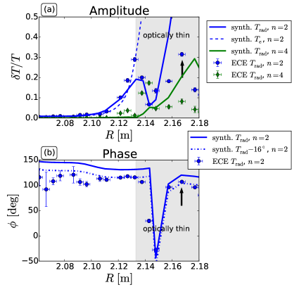
Figure 15: $\#30839$, (a) relative amplitude of the $n=2$ (blue) and $n=4$ (green) component from synthetic $T\rm{{}_{rad}}$ (solid), and ECE measurements (circle) as well as only $n=2$ from synthetic $T\rm{{}_{e}}$ (dashed). (b) phase of $n=2$ from synthetic $T\rm{{}_{rad}}$ and ECE . The phases systematically deviate by around $16^{\circ}$ indicated by the dash-dotted line. Channels in the optically thin region can significantly distort the amplitude and phase analysis.

In contrast to the amplitude comparison, the phase information is less dependent on the radial position. The boundary perturbation around the LFS midplane has a relatively large poloidal extension and the distortion penetrates straightly from the edge towards the core (see Fig. 13(b)). Thus, the phase is not changing much along the ECE LOS within the optically thick region ($R<2.13\ \rm{m}$). This is seen in the ECE measurements and confirmed by the synthetic $T\rm{{}_{rad}}$ data (Fig.  15(b)). Moreover, the synthetic $T\rm{{}_{rad}}$ successfully describes the phase flip at the edge ($R\approx 2.14-2.15\ \rm{m}$), which is caused by the interplay between the displacement and the non-monotonic characteristics of the $T\rm{{}_{rad}}$ profile. Channels viewing only the optically thin plasma also contain the phase information from the pedestal. The ECE channels in the SOL, that show a strong $n=2$ component (one is indicated by an arrow in Fig. 15), observe almost the same phase as the pedestal channels ($R\approx 2.12\ \rm{m}$). This is expected because they measure the down-shifted radiation of the electrons in the pedestal region. Slight differences in the phase between these channels in the optically thick and thin region (e.g. arrow in Fig. 15) can occur, because their ray paths differ slightly as well. The reason for this lies in the different measurement frequencies (see Sec. 2.3), which can have an impact on the ray refraction.

The phase profile of ECE $T\rm{{}_{rad}}$ and synthetic $T\rm{{}_{rad}}$ shows a systematic offset of $\Delta\phi\approx 16^{\circ}$ between them (indicated by the dash-dotted line in Fig. 15(b)). This offset can be explained by the PSL response. The MP-coils are mounted close to the PSL. Since it is a copper conductor, image currents in the PSL can screen transient magnetic fields produced by the MP-coils. Thus, the PSL acts similar to $L/R$ lowpass filter and delays the rigid rotation [32]. Although the MP-field was rotated by only $0.5\;\rm{Hz}$, the PSL causes a measurable phase delay with respect to the applied coil current. This is also inline with newly employed finite elements calculations of the MP-coils and the PSL, which predict a phase delay in the midplane of $\Delta\phi\rm{{}_{upper}}\approx 14.3^{\circ}$ regarding the upper coil set and $\Delta\phi\rm{{}_{lower}}\approx 11.2^{\circ}$ for the lower one [30, 33]. The phase delay of the upper and lower coil set is different because of the different geometry with respect to the PSL.

5.2 Comparison using profile diagnostics

In the previous section, we used the amplitude information from single channels to compare it with synthetic data. But it is also possible to use the information from the entire edge profile. The displacement can be directly obtained by the radial shift between two profiles at the time of the maximum and the minimum displacement. Moreover, it also allows us to compare the displacement between the different profile diagnostics even if the measured plasma parameters are not the same. Figure 16 shows ECE, CXRS and LIB profiles at the time of maximum and minimum displacement. The corresponding synthetic data are also plotted. Due to the different toroidal and poloidal arrangement of the diagnostics, the times of the maximum and minimum vary for the different diagnostics. In general, the agreement between the synthetic and the measured profiles is good. To get one quantity for the displacement, first, we fit the profiles at the maximum displacement using a spline. Then, this spline is only varied by a radial shift until the LSQ is minimized using the data at the minimum displacement. This is relatively robust and the uncertainties due to the change in the gradients are also reflected in the uncertainties of the determined shift. Because of the ’shine-through’ and dominating passive lines, the ECE and the CXRS data from the SOL are not used for this procedure. The same procedure was also applied to the synthetic data generated from the VMEC equilibrium. The displacements derived from this method are given in the left bottom corner of each frame in Fig. 16. ECE and CXRS deliver very similar displacements, but they exhibit slightly larger values than predicted by VMEC. In the case of LIB, this difference between the measured and the synthetic data is more pronounced.

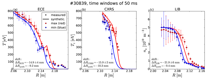
Figure 16: $\#30839$, profiles from (a) ECE (b) CXRS and (c) LIB. Measured (circles) and synthetic (solid) profiles at the maximum (red) and minimum displacement (blue) of each diagnostic. The analyzed time windows are $50\ \rm{ms}$. The derived displacements are given in the left bottom corner. ECE and CXRS observe the same displacement, whereas the one measured by LIB is slightly larger.

Unlike ECE and CXRS, the LIB diagnostic is well-suited for determining changes of the separatrix position. Assuming a constant separatrix density during the rigid rotation, the separatrix position can be easily tracked along the LIB. We determine the separatrix density using the density profile prior to the MP onset ($n_{e,sep}\approx 1.3\cdot 10^{19}\ \rm{m^{-3}}$ from Fig. 5(a)). Figure 17 illustrates (i) the separatrix position determined from the LIB diagnostic , (ii) the outermost boundary of the VMEC equilibrium and (iii) the boundary from the vacuum field approximation is indicated by the color scaling using the connection length $L_{c}$ of the stable manifold (see Ref. [18]). Both, (ii) and (iii) are calculated along the LIB. The displacement from the VMEC equilibrium exceeds the prediction from vacuum field calculations by a few millimeters. The sinusoidal is well seen in the measurements and agrees qualitatively. This comparison indicates a larger displacement than predicted by VMEC and is also consistent with the measurements shown in Fig. 17.

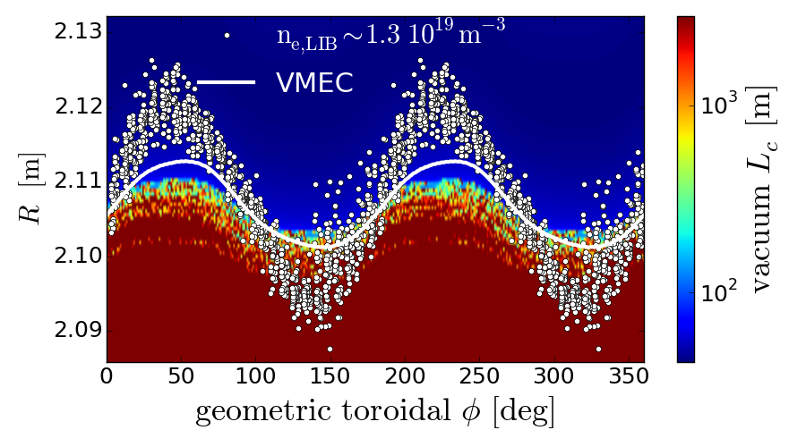
Figure 17: $\#30839$, circles are the estimated separatrix from LIB using a density of $1.3\cdot 10^{19}\ \rm{m^{-3}}$. Solid line is the outermost flux surface from VMEC along the LIB LOS and the color scaling indicates the connection length $L_{C}$ using the vacuum field approximation. LIB data exceeds the VMEC and the vacuum field calculations. LIB data is shifted radially inwards by $2\ \rm{mm}$.

5.3 Discussion of the amplitude comparison

A quantitative amplitude comparison using single ECE channels is challenging due to the dependencies on the measurement positions and the ’shine-through’ effect. Small variations in the position can have large influence on its interpretation. Despite these difficulties, the decay of the distortion towards the plasma core agrees very well between the ECE $T\rm{{}_{rad}}$ and the synthetic $T\rm{{}_{rad}}$. The displacement can be analyzed using the relative amplitude from single channels. This method makes a comparison between different diagnostics difficult, because they measure different plasma parameters. A comparison to e.g. VMEC requires the development of synthetic diagnostics. Thus, it is more useful to determine the displacement by aligning the entire edge profiles. This allows us to compare directly and quantitively the measured displacement not only to others diagnostics, but also to 3D equilibrium codes.

All edge profile diagnostics around the LFS midplane exhibit a displacement, which is slightly larger than predicted by the VMEC equilibrium and thus, larger than calculated in the vacuum field approximation as well (see Fig. 17). In principle, the plasma position control could artificially amplify or mitigate the distortion. This depends on the relative phase between the position of the $B_{\Theta}$ arrays and the used profile diagnostics (discussed in Ref. [22]). We can exclude this in the midplane for two reasons. First, CXRS and 1D-ECE measure the same amplitude at different toroidal phases (see time traces in Fig. 4). Second, the CXRS system is in the midplane on the opposite side of the $B_{\Theta}$ array (see Fig. 2). A feedback controlled system solely based on measurements of one toroidal position would counteract the 3D distortion [22] and, therefore, the modulation at the position of the CXRS system would be compensated. Because of the fact that the displacement from edge CXRS also exceeds the prediction from VMEC (see Fig. 16(b)), we assume that the plasma position control system does not artificially amplify the measured modulation in the midplane. The position control system of ASDEX Upgrade also uses toroidal flux loops for the feedback control system, which seem to mitigate the effect of the MP-field on the control system in comparison to other devices like MAST [22]. However, small changes in the shape due to the control system can certainly not be excluded, which could explain that LIB measures a larger displacement than CXRS and ECE.

VMEC seems to slightly underestimate the displacement in the midplane. A quantitive comparison of MARS-F employing the resistive as well as the ideal MHD model with VMEC using the identical inputs show very similar displacement values. This indicates that the used input parameters can also be responsible for this underestimation. As already mentioned in section 4.4, the used pressure profile was determined by aligning various diagnostics at one time point during the MP-phase. The resulting total pressure has experimental uncertainties because the used profile diagnostics are toroidally separated. As shown in Fig. 5, the gradients can vary depending on the toroidal phase. Since the amplitude of the displacement or rather the stable ideal kink modes are driven by the edge pressure gradient and the associated bootstrap current, a lower input pressure gradient can lead to a smaller displacement in MHD equilibrium codes. This sensitivity should be kept in mind. For further details on the sensitivity of the displacement on the pressure profile and hence, the plasma beta, we refer to the sensitivity studies in Ref. [14, 62].

6 Poloidal mode structure comparison

The measured displacement and the one from VMEC exceed the prediction from the vacuum field calculations. This indicates the presence of a kink response, which amplifies the magnetic perturbations and thus, the displacement. According to plasma response calculations, these amplified magnetic perturbations show dominant non-resonant components ($|m|>|nq|$). To investigate if this non-resonant behavior is also seen in the ECE-I system, we make use of its poloidal resolution and compare the measured data to VMEC calculations.

6.1 ECE-I vis-a-vis VMEC

Figure 18 shows the comparison between the measured (diamonds) and the synthetic ECE-I (circles) data. To avoid corruption from the ’shine-through’ well, channels are discarded which measure a significant ’$n=4$’ (${\delta T\rm{{}_{rad}}}/{T\rm{{}_{rad}}}(n=4)>0.05$) component. We only use channels with a significant $n=2$ component (${\delta T\rm{{}_{rad}}}/{T\rm{{}_{rad}}}(n=2)>0.085$). The few channels, which have permanently their cold resonance position in the optically thin region and fulfill the mentioned conditions, are also taken into account (green diamonds).

All selected channels from ECE-I and their corresponding synthetic channels are fitted using the LSQ fit of a sine function including higher harmonics. The $\rho_{pol}$ values of the used channels range from $0.95$ to $0.981$. Their mean value is $0.968$, which is the $q\approx-5.35$ surface. To compare the poloidal mode structure between the measurements and the synthetic data, we plot the SFL angles of the channels using the $q=-5.35$ surface ($\Delta\Theta^{\star}_{q=-5.35}$) of the CLISTE equilibrium versus the phase determined from the sine fits in Fig. 18. The ’warm’ resonance position is used to calculate $\Delta\Theta^{\star}_{q=-5.35}$ for channels with their cold resonance position in the optically thick (blue diamonds) and thin (green diamonds) region. The measured data agree very well with the synthetic data. The poloidal mode number of both is determined by fitting a linear function to the individual datasets (Fig. 18). From the slope of this linear function, we get $m_{ECE-I}={\Delta\phi}/\Delta\Theta^{\star}_{q=-5.35}=9.83\pm 0.98$ using ECE-I and $m_{synth}=10.72\pm 0.63$ using synthetic data. Using only the ECE-I channels in the optically thick does not strongly change the result. There is a small difference between the prediction and the measurements, but it is within the uncertainties. Furthermore, one should also keep in mind that the $q$-profile contains also uncertainties, since the initial equilibrium calculation is constrained by measured density and temperature profiles.

The synthetic and the measured data indicate an almost resonant response at the $q=-5.35$ surface ($m_{pitch}\approx 10.7$). In fact, $m_{ECE-I}$ tends to be even lower than the pitch aligned mode number. This is in contradiction to the non-resonant response with $|m|>|nq|$ expected from the magnetic perturbation. This seeming discrepancy originates from a difference in the poloidal mode structure between the magnetic perturbation and the flux surface displacement, which will be discussed in the following section.

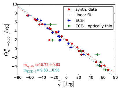
Figure 18: $\#30839$, SFL angle using the $q=-5.35$ flux surface versus the derived phase delay using $\widetilde{\phi}=\phi\ -<\phi>$. ECEI data from optically thick (blue diamonds) and thin (green diamonds) plasma regions agree with synthetic data from VMEC (red circles). The poloidal mode numbers $m$ (left bottom corner) are determined from the slope of the linear fits (dashed).

6.2 Displacement versus magnetic perturbation

To compare the flux surface displacement with the magnetic perturbation, we use a modified version of the MFBE code [63] (described in [64]) to calculate the magnetic perturbation. In the following, we compare the mode spectra between the magnetic perturbation and the displacement predicted by VMEC and MARS-F using ideal MHD. For comparative purposes, Fig. 19(a) and 19(d) show the vacuum field perturbation using the coordinate system from VMEC and MARS-F, respectively. The perturbation of the equilibrium field, which is the sum of the vacuum field and the plasma response field perturbation is plotted in Fig. 19(b) and 19(e).

The equilibrium field perturbation predicted by VMEC as well as MARS-F is lowest around the resonant surfaces, which is expected from ideal MHD (Fig. 19(b) and (e)). Both calculations show a kink response situated at $|m|>|nq|$, which amplifies the field perturbation. This has been reported previously [15, 17, 65, 61] and has also been experimentally verified using probe measurements [17, 66]. On the contrary, the poloidal mode spectra of the flux surface displacement does not indicate such pronounced non-resonant components (Fig. 19(c) and (f)). The structures are almost pitch aligned [67]. The calculations from MARS-F and VMEC of the radial displacement are in good agreement and they are also in-line with the ECE-I measurements (white diamond) within their uncertainties. The amplitudes of the displacement from both codes agree quantitatively, whereas the equilibrium field perturbations agree qualitatively. Deviations from exactly zero resonant components at rational surfaces due to ideal MHD can arise e.g. from numerical limitations and/or from the treatment of sheet currents on rational surfaces [68]. Detailed quantitative comparisons between MARS-F and VMEC are beyond the scope of this paper.

The analysis of the poloidal mode spectra of the flux surface displacement using ECE-I and its comparison to the 3D MHD equilibrium codes is relatively advanced. Its correctness relies on the accuracy of the individual steps like the modeling of the electron cyclotron radiation transport, the determination of the ’warm’ resonance position, the calculation of the SFL coordinate and thus, of the poloidal mode spectra, etc. Figure 19(c) shows the poloidal mode spectra of the displacement from VMEC. To demonstrate the consistency of the entire analysis chain, we also plot the dominant poloidal mode number determined using the synthetic ECE-I diagnostic generated from the VMEC equilibrium (black rectangular) in Fig. 19(c). The point from the synthetic diagnostic overlies almost exactly the maxima of the poloidal mode spectra, which underlines the consistency and correctness of this analysis.

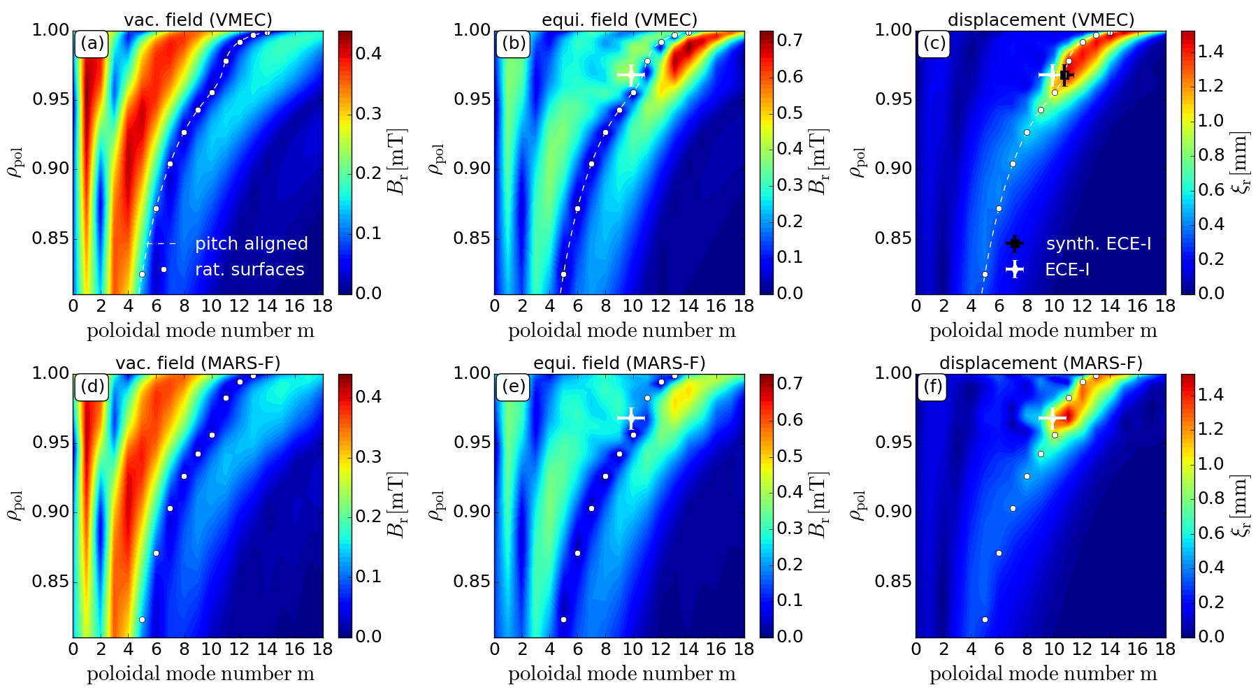
Figure 19: The $n=-2$ poloidal mode spectrum of (a) the vacuum field perturbation, (b) the equilibrium field perturbation, (c) the radial displacement from VMEC and (d) vacuum field perturbation (e) equilibrium field perturbation, (f) displacement from MARS-F. Note, there is no difference in the color scaling between VMEC and MARS-F. Poloidal mode number obtained from ECE-I is plotted (white diamond) as well as from the synthetic ECE-I (black square) in (c) to underline the consistency. The difference in the poloidal mode spectrum between the plasma response field and the displacement is apparent in both codes.

6.3 Discussion of the poloidal mode structure

While the calculated poloidal mode structure of the MP is non-resonant, the measured displacement using ECE-I shows an almost resonant response. This is a seeming contradiction, since the equilibrium field is the important parameter, which determines the displacement. Hence, one would expect that they have the same poloidal mode structure. But In the following, we will briefly show that this difference can already be explained by simple ideal MHD calculations.

In linear MHD, the linearized magnetic perturbation $\vec{B}=\vec{B_{0}}+\vec{B_{1}}$ is related to the surface displacement $\vec{\xi}$ via [69]:

$$\vec{B_{1}}=\vec{\nabla}\times(\vec{\xi}\times\vec{B_{0}}).$$ (2)

Assuming a cylindrical plasma ($r,\Theta,z$), the radial displacement $\xi_{r}$ and the radial magnetic field perturbation $B_{r}$ normal to the axisymmetric flux surface relate:

$$B_{r}=\frac{B_{\Theta}}{r}\frac{\partial\xi_{r}}{\partial\Theta}+B_{\phi}\frac{\partial\xi_{r}}{\partial z},$$ (3)

where $B_{\Theta}$ and $B_{\phi}$ are the poloidal and toroidal magnetic component, respectively. Using a periodic distortion $\xi\rm{{}_{r}}=\xi_{a}\ e^{i(m\Theta-\frac{n}{R}z)}$ and the resonant condition $q=\frac{m}{n}=\frac{r}{R}\frac{B_{\phi}}{B_{\Theta}}$, one gets the following relation at rational surfaces:

$$B_{r}=i\frac{B_{\Theta}}{r}\left(m-nq\right)\xi_{r}\rightarrow\xi_{r}\propto\frac{B_{r}}{m-nq}$$ (4)

Consequently, $\xi_{r}$ maximizes at resonant surfaces in cylindrical plasmas. In the case of an elongated toroidal plasma, the elongated shape causes additional poloidal coupling between the different harmonics $\Delta m=0,1,2$. Then, the relation between $B_{r}$ and $\xi_{r}$ (Equ. 4) is not a relation between individual harmonics anymore. Nevertheless, the $\frac{1}{m-nq}$ dependence in Equ. 4 is still the underlying reason for $\xi_{r}$ to be maximized at resonant surfaces, which is underlined by VMEC and MARS-F calculations (Fig. 19(c,f)). This is also in-line with a new class of 3D ideal-MHD equilibria with nested surfaces and with current sheets at resonant surfaces producing a jump in the $q$-profile [70].

In summary, linear perturbative ideal MHD calculations give a reasonable explanation for the differences in the mode structure between the surface displacement and magnetic perturbation. Initially, one idea of measuring the poloidal mode number was to distinguish resonant resistive MHD response from non-resonant ideal MHD response. Since this non-resonant ideal MHD response appears practically resonant in the displacement, this method is not suitable to disentangle resistive from ideal MHD response.

7 Conclusions and summary

The combination of a rigid rotating MP-field and toroidally localized diagnostics provide a useful tool to measure the plasma surface distortion. This analysis relies on stable plasma conditions during the rigid rotation. ECE diagnostics deliver informations about the plasma response via the flux surface displacement within the confined region, whereas ECE measurements around the separatrix are difficult to interpret due to the transition from an optically thick to an optically thin plasma. Additional oblique angles of the LOS complicate the interpretation of the ECE data. It is therefore necessary to combine ray tracing with forward modeling of the radiation transport. The calculation of the ’warm’ resonance positions (calculated maximum of the observed intensity distribution) is useful to estimate the real measurement position. The ideal MHD equilibrium code VMEC was used to model the 3D plasma surface displacement and synthetic diagnostics were developed to compare the measurements with VMEC.

A quantitative comparison of the displacement amplitude appears to be challenging. One can either use the single channel information and/or the entire profile information for the comparison. The first one is easier to realize, but implies the difficulties of the large sensitivity on the measurement position and of the incomparability between the various profile diagnostics. Hence, we conclude that the use of the entire profile appears to be more useful. The comparisons of the displacement between synthetic and measured data are in reasonable agreement. The modeling underestimates only slightly the amplitude of the distortion on the LFS midplane. Since MARS-F and VMEC exhibit very similar displacements, one plausible explanations for this minor underestimation could also be the uncertainties in the input parameters, like the pressure profile or the shape of the input equilibrium [71]. One should also keep in mind the role of the plasma position control during the rigid rotation. In the case of ASDEX Upgrade, the effect of the control system seems to be relatively small in the midplane due to the implementation of toroidal flux loops in the used reconstruction. In conclusion, not only the measurements of the amplitude require a careful treatment, but also the input parameters for the modeling in the presence of non-axisymmetric MPs.

The analysis of ECE-I shed some light onto the plasma response in terms of the flux surface displacement in the pedestal region and its poloidal mode structure. Differences in the poloidal mode structure between the magnetic perturbations and the flux surface displacement are predicted by MARS-F and VMEC. The magnetic perturbation of the equilibrium field (vacuum field plus plasma response field) is non-resonant ($|m|>|nq|$), whereas the displacement is almost resonant ($|m|\approx|nq|$) as measured by ECE-I and as expected from ideal MHD in the vicinity of rational surfaces. Hence, it is not possible to use the poloidal mode number from the displacement to disentangle ideal from resistive MHD response (resistive is always resonant).

The impact of the pressure profile and the differential phase angle $\Delta\phi\rm{{}_{ul}}$ on the displacement amplitude, although experimentally challenging, will be subject of future investigations.

8 Acknowledgement

The authors would like to thank V. Igochine and E. Wolfrum for fruitful discussions. F. M. Laggner is a fellow of the Friedrich Schiedel Foundation for Energy Technology. This work has been carried out within the framework of the EUROfusion Consortium and has received funding from the Euratom research and training programme 2014-2018 under grant agreement No 633053. The views and opinions expressed herein do not necessarily reflect those of the European Commission.

References

- [1] T. E. Evans et al. Suppression of Large Edge-Localized Modes in High-Confinement DIII-D Plasmas with a Stochastic Magnetic Boundary. Physical Review Letters, 92:235003, June 2004.
- [2] Y. Liang et al. Active Control of Type-I Edge-Localized Modes with Perturbation Fields in the JET Tokamak. Physical Review Letters, 98:265004, June 2007.
- [3] W. Suttrop et al. First Observation of Edge Localized Modes Mitigation with Resonant and Nonresonant Magnetic Perturbations in ASDEX Upgrade. Physical Review Letters, 106(22):225004, 2011.
- [4] T. E. Evans et al. RMP ELM suppression in DIII-D plasmas with ITER similar shapes and collisionalities. Nuclear Fusion, 48(2):024002, 2008.
- [5] Y. Sun et al. Modeling of non-axisymmetric magnetic perturbations in tokamaks. Plasma Physics and Controlled Fusion, 57(4):045003, 2015.
- [6] Y. M. Jeon et al. Suppression of Edge Localized Modes in High-Confinement KSTAR Plasmas by Nonaxisymmetric Magnetic Perturbations. Physical Review Letters, 109:035004, 2012.
- [7] A. Kirk et al. Understanding edge-localized mode mitigation by resonant magnetic perturbations on MAST. Nuclear Fusion, 53(4):043007, 2013.
- [8] W. Suttrop et al. Studies of magnetic perturbations in high confinement mode plasmas in asdex upgrade. AEA Int. Conf. on Fusion Energy (St Petersburg, Russia, 2014) EX/P1-23, 2014.
- [9] A. Kirk et al. Effect of resonant magnetic perturbations on low collisionality discharges in MAST and a comparison with ASDEX Upgrade. Nuclear Fusion, 55(4):043011, 2015.
- [10] M. Garcia-Munoz et al. Fast-ion losses induced by ELMs and externally applied magnetic perturbations in the ASDEX Upgrade tokamak. Plasma Physics and Controlled Fusion, 55(12):124014, 2013.
- [11] C. Paz-Soldan et al. Observation of a Multimode Plasma Response and its Relationship to Density Pumpout and Edge-Localized Mode Suppression. Physical Review Letters, 114:105001, 2015.
- [12] Y. Q. Liu et al. Feedback stabilization of nonaxisymmetric resistive wall modes in tokamaks. I. Electromagnetic model. Physics of Plasma, 7(9):3681, 2000.
- [13] F. Orain et al. Non-linear MHD modeling of edge localized mode cycles and mitigation by resonant magnetic perturbations. Plasma Physics and Controlled Fusion, 57(1):014020, 2015.
- [14] E. Strumberger et al. MHD instabilities in 3D tokamaks. Nuclear Fusion, 54(6):064019, 2014.
- [15] D. A. Ryan et al. Toroidal modelling of resonant magnetic perturbations response in ASDEX-Upgrade: coupling between field pitch aligned response and kink amplification. Plasma Physics and Controlled Fusion, 57(9):095008, 2015.
- [16] F. Orain, M. Hoelzl, E. Viezzer, M. Dunne, M. Becoulet, P. Cahyna, G. T. A. Huijsmans, J. Morales, M. Willensdorfer, W. Suttrop, A. Kirk, S. Pamela, E. Strumberger, S. Guenter, A. Lessig, the ASDEX Upgrade Team, and the EUROfusion MST1 Team. Non-linear modeling of the plasma response to RMPs in ASDEX Upgrade. submitted to Nuclear Fusion, February 2016.
- [17] M J Lanctot et al. Measurement and modeling of three-dimensional equilibria in DIII-D. Physics of Plasma, 18(5):056121, 2011.
- [18] R. A. Moyer et al. Measurement of plasma boundary displacement by n= 2 magnetic perturbations using imaging beam emission spectroscopy. Nuclear Fusion, 52(12):123019, 2012.
- [19] M. W. Shafer et al. Plasma response measurements of non-axisymmetric magnetic perturbations on DIII-D via soft x-ray imaginga). Physics of Plasmas (1994-present), 21(12):–, 2014.
- [20] Y. Q. Liu et al. Toroidal modelling of RMP response in ASDEX Upgrade: coil phase scan, q95 dependence, and toroidal torques. accepted in NF, 2016.
- [21] I. T. Chapman et al. Three-dimensional corrugation of the plasma edge when magnetic perturbations are applied for edge-localized mode control in MAST. Plasma Physics and Controlled Fusion, 54(10):105013, 2012.
- [22] I. T. Chapman et al. The effect of the plasma position control system on the three-dimensional distortion of the plasma boundary when magnetic perturbations are applied in MAST. Plasma Physics and Controlled Fusion, 56(7):075004, 2014.
- [23] B. J. Tobias et al. Boundary perturbations coupled to core 3/2 tearing modes on the DIII-D tokamak. Plasma Physics and Controlled Fusion, 55(9):095006, 2013.
- [24] B. J. Tobias et al. Non-axisymmetric magneto- hydrodynamic equilibrium in the presence of internal magnetic islands and external magnetic perturbation coils. Plasma Physics and Controlled Fusion, 55(12):125009, 2013.
- [25] J. K. Park et al. Computation of three-dimensional tokamak and spherical torus equilibria. Physics of Plasma, 14(5), 2007.
- [26] S. K. Rathgeber et al. Estimation of edge electron temperature profiles via forward modelling of the electron cyclotron radiation transport at ASDEX Upgrade. Plasma Physics and Controlled Fusion, 55(2):025004, 2013.
- [27] S. P. Hirshman et al. Three-dimensional free boundary calculations using a spectral Green’s function method. Computer Physics Communications, 43(1):143–155, 1986.
- [28] R. Fischer et al. Spatiotemporal response of plasma edge density and temperature to non-axisymmetric magnetic perturbations at ASDEX Upgrade. Plasma Physics and Controlled Fusion, 54(11):115008, 2012.
- [29] J. C. Fuchs et al. Investigation of the boundary distortions in the presence of rotating external magnetic perturbations on ASDEX Upgrade. 41th EPS Conference on Plasma Phys., 2014.
- [30] W. Suttrop et al. In-vessel saddle coils for MHD control in ASDEX Upgrade. Fusion Engineering and Design, 84(2–6):290–294, 2009.
- [31] M. Teschke et al. Electrical Design Of The Inverter System BUSSARD For ASDEX Upgrade Saddle Coils. Fusion Engineering and Design / 28th Symposium on Fusion Technology (SOFT 2014), 2014.
- [32] W. Suttrop et al. Physical description of external circuitry for Resistive Wall Mode controlin ASDEX Upgrade. 36th EPS Conference on Plasma Phys. Sofia, 33E:1–4, 2009.
- [33] W. Suttrop. Finite elements calculations from the saddle coils and the PSL. private communication, 2016.
- [34] W. Suttrop et al. Studies of edge localized mode mitigation with new active in-vessel saddle coils in ASDEX Upgrade. Plasma Physics and Controlled Fusion, 53(12):124014, 2011.
- [35] M. Maraschek et al. Measurement and impact of the n=1 intrinsic error field at ASDEX Upgrade. 40th Conf.EPS Plasma Phys. (Espoo, 1–5 July 2013), 2014.
- [36] E. Viezzer et al. High-resolution charge exchange measurements at ASDEX Upgrade. Review of Scientific Instruments, 83(10):103501, 2012.
- [37] M. Willensdorfer et al. Improved chopping of a lithium beam for plasma edge diagnostic at asdex upgrade. Review of Scientific Instruments, 83(2):023501, 2012.
- [38] M. Willensdorfer et al. Characterization of the Li-BES at ASDEX Upgrade. Plasma Physics and Controlled Fusion, 56(2):025008–10, January 2014.
- [39] B. Carli. Design of a Blackbody Reference Standard for the Submillimeter Region. Microwave Theory and Techniques, IEEE Transactions on, 22(12):1094–1099, 1974.
- [40] H. J. Hartfuss et al. Heterodyne methods in millimetre wave plasma diagnostics with applications to ece, interferometry and reflectometry. Plasma Physics and Controlled Fusion, 39(11):1693, 1997.
- [41] I. Classen et al. 2D electron cyclotron emission imaging at ASDEX Upgrade (invited). Review of Scientific Instruments, 81(10):10D929–6, 2010.
- [42] I. Classen et al. Dual array 3D electron cyclotron emission imaging at ASDEX Upgradea). Review of Scientific Instruments, 85(11), 2014.
- [43] Y. Gao et al. Effects of 3D magnetic perturbation on divertor heat load redistribution on ASDEX Upgrade . 42nd EPS Conference on Plasma Phys. Lissabon, 39E:1–4, 2015.
- [44] P. J. McCarthy et al. Identification of edge-localized moments of the current density profile in a tokamak equilibrium from external magnetic measurements. Plasma Physics and Controlled Fusion, 54(1):015010, 2012.
- [45] A. D. Turnbull et al. Plasma response models for non-axisymmetric perturbations. Nuclear Fusion, 52(5):054016, 2012.
- [46] R. Fischer et al. Integrated data analysis of profile diagnostics at asdex upgrade. Fusion science and technology, 58(675–682), 2010.
- [47] W. D. D’haeseleer. Flux Coordinates and Magnetic Field Structure. Springer-Verlag, Berlin, 1991.
- [48] M Bornatici, R Cano, O de Barbieri, and F Engelmann. Electron cyclotron emission and absorption in fusion plasmas. Nuclear Fusion, 23(9):1153, 1983.
- [49] G D Garstka, R F Ellis, and M E Austin. A flexible, broadband ECE diagnostic for DIII-D. Fusion Engineering and Design, 53(1–4):97–103, 2001.
- [50] N. B. Marushchenko et al. Ray tracing simulations of ecr heating and ece diagnostic at w7-x stellarator. Plasma and Fusion Research, 2:S1129–S1129, 2007.
- [51] S. S. Denk et al. Radiation transport modelling for the interpretation of oblique ECE measurements. submitted to Plasma Physics and Controlled Fusion, 2016.
- [52] E. Poli et al. TORBEAM, a beam tracing code for electron-cyclotron waves in tokamak plasmas. Computer Physics Communications, 136(1–2):90–104, 2001.
- [53] M. Sato et al. Relativistic Down-Shift Frequency Effect on the Application of Electron Cyclotron Emission Measurements to Medium Temperature Tokamak Plasmas. Japanese Journal of Applied Physics, 34(6A):L708, 1995.
- [54] B. J. Tobias et al. ECE-imaging of the H-mode pedestal (invited). Review of Scientific Instruments, 83(10), 2012.
- [55] S. P. Hirshman et al. Steepest-descent moment method for three-dimensional magnetohydrodynamic equilibria. Physics of Fluids, 26(12):3553, 1983.
- [56] M. G. Dunne et al. Measurement of neoclassically predicted edge current density at ASDEX Upgrade. Nuclear Fusion, 52(12):123014, 2012.
- [57] J. L. Johnson et al. Numerical determination of axisymmetric toroidal magnetohydrodynamic equilibria. Journal of Computational Physics, 32(2):212–234, 1979.
- [58] Hartmut Zohm. Magnetihydrodynamic Stability of Tokamaks. John Wiley and Sons, 2014.
- [59] A. H. Boozer et al. Establishment of magnetic coordinates for a given magnetic field. Physics of Fluids, 25(3):520, July 1981.
- [60] E. Viezzer et al. Evidence for the neoclassical nature of the radial electric field in the edge transport barrier of asdex upgrade. Nuclear Fusion, 54(1):012003, 2014.
- [61] S. R. Haskey et al. Linear ideal MHD predictions for n = 2 non-axisymmetric magnetic perturbations on DIII-D. Plasma Physics and Controlled Fusion, 56(3):035005, 2014.
- [62] C. Paz-Soldan et al. Equilibrium drives of the low and high field side n = 2 plasma response and impact on global confinement. Nuclear Fusion, 56(5):056001, 2016.
- [63] E. Strumberger et al. Finite-β magnetic field line tracing for helias configurations finite-β magnetic field line tracing for helias configurations. Nuclear Fusion, 37(19), 1997.
- [64] E. Strumberger et al. Numerical computation of magnetic fields of two- and three-dimensional equilibria with net toroidal current. Nuclear Fusion, 42(7):827, 2002.
- [65] M J Lanctot et al. Sustained suppression of type-I edge-localized modes with dominantly n = 2 magnetic fields in DIII-D. Nuclear Fusion, 53(8):083019, 2013.
- [66] J. D. King et al. Three-dimensional equilibria and island energy transport due to resonant magnetic perturbation edge localized mode suppression on DIII-D. Physics of Plasma, 22(11), 2015.
- [67] Samuel A Lazerson, Joaquim Loizu, Steven Hirshman, and Stuart R Hudson. Verification of the ideal magnetohydrodynamic response at rational surfaces in the VMEC code. Physics of Plasma, 23(1):012507, 2016.
- [68] A. Reiman et al. Tokamak plasma high field side response to an n = 3 magnetic perturbation: a comparison of 3D equilibrium solutions from seven different codes. Nuclear Fusion, 55(6):063026, 2015.
- [69] J. Freidberg. Ideal MHD, page 337. Cambridge University Press, 2014.
- [70] J. Loizu. et al. Pressure-driven amplification and penetration of resonant magnetic perturbations. Physics of Plasma, 23(5), 2016.
- [71] L. Li et al. Modelling plasma response to RMP fields in ASDEX-Upgrade with varying edge safety factor and triangularity. submitted to Nuclear Fusion, 2016.