Analysis of Interference Correlation in Non-Poisson Networks

Abstract

The correlation of interference has been well quantified in Poisson networks where the interferers are independent of each other. However, there exists dependence among the base stations (BSs) in wireless networks. In view of this, we quantify the interference correlation in non-Poisson networks where the interferers are distributed as a Matern cluster process (MCP) and a second-order cluster process (SOCP). Interestingly, it is found that the correlation coefficient of interference for the Matern cluster networks, $\zeta_{MCP}$, is equal to that for second-order cluster networks, $\zeta_{SOCP}$. Furthermore, they are greater than their counterpart for the Poisson networks. This shows that clustering in interferers enhances the interference correlation. In addition, we show that the correlation coefficients $\zeta_{MCP}$ and $\zeta_{SOCP}$ increase as the average number of points in each cluster, $c$, grows, but decrease with the increase in the cluster radius, $R$. More importantly, we point that the effects of clustering on interference correlation can be neglected as $\frac{c}{\pi^{2}R^{2}}\rightarrow 0$. Finally, the analytical results are validated by simulations.

I Introduction

Interferers in wireless networks are both temporally and spatially correlated since they are subject to finite mobility and real network deployment. This leads to the correlation in interference [1, 2, 3]. Such correlation significantly affects the performance of systems with retransmission schemes, cooperative relaying, and multiple antennas [4]. Thus, it is important to quantify the interference correlation. However, traditional analysis focuses on the interference correlation caused by the temporally correlated interferers.

Ganti and Haenggi are among the first to quantify the interference correlation in Poisson networks in terms of correlation coefficient [5]. They found that there exists spatio-temporal interference correlation in wireless networks due to the slow node mobility. Such correlation reduces the diversity of networks with retransmissions [6] or multi-antenna receivers [7], and thus degrades the corresponding network performance. Increasing node mobility [8], the randomness in fading [5] and MAC protocols [9] can reduce the interference correlation. Note that prior analysis was conducted on one-tier Poisson networks. The authors in [10, 11] investigated the interference correlation in heterogeneous cellular networks (HCNs) where the BSs follow multiple independent Poisson point processes (PPPs). Except for the aforementioned research, prior work related to Poisson networks [5, 6, 7, 8, 9, 10] only addresses the interference correlation caused by the temporally correlated interferers, since the assumption of Poisson distribution inherently neglects the spatial correlation in BS locations.

There exists dependence including clustering and repulsion among the BS locations, especially for HCNs. Specifically, low power nodes are always allocated in groups to provide high capacity in hotspots. Furthermore, they are deployed in the annular region of macrocells to avoid severe inter-tier interference [12, 13]. We call these two phenomenons as intra-tier dependence (i.e., the clustering among the BSs within the same tier) and inter-tier dependence (i.e., the repulsion among the BSs belonging to different tiers), respectively. Considering the intra-tier dependence, a Matern cluster process (MCP) is promising for modeling the clustered low-power BSs in HCNs due to its analytical tractability [14, 15, 16]. Given both the intra- and inter-tier dependence, the authors in [17] modeled the low-power BSs as a second-order cluster process (SOCP) and analyzed the corresponding network performance. The resultant spatial correlation among the BSs makes the interference correlation more complex, which has not been investigated in the literature.

In this paper, we quantify the interference correlation caused by the spatial correlation of interferers in terms of interference correlation coefficient. For simplicity, let $\zeta_{PPP}$, $\zeta_{MCP}$, and $\zeta_{SOCP}$ denote the spatio-temporal interference correlation coefficients in the cases where the interferers are distributed as a PPP, MCP, and SOCP, respectively. The mean numbers of points in each cluster of MCP and SOCP are represented as $c$ and $c_{2}$, respectively. Moreover, the radiuses of a typical cluster of MCP and SOCP are denoted as $R$ and $D_{2}$, respectively. The main contributions of this paper are summarized as follows.

• The interference correlation coefficients, $\zeta_{MCP}$ and $\zeta_{SOCP}$, are derived and shown to be greater than $\zeta_{PPP}$. This implies that there exist positive contributions of clustering on interference correlation. In particular, the contributions of clustering in these two cases are the same, i.e., $\zeta_{MCP}=\zeta_{SOCP}$, if $c=c_{2}$ and $R=D_{2}$.

• The correlation coefficients $\zeta_{MCP}$ and $\zeta_{SOCP}$ are found to be significantly affected by the average number of points in each cluster, $c$, and the radius of a typical cluster, $R$. Moreover, it is proved that increasing $c$ or decreasing $R$ enhances the interference correlation, and vice versa. In addition, $\zeta_{MCP}$ and $\zeta_{SOCP}$ are approximately equal to $\zeta_{PPP}$ in the case of $\frac{c}{\pi^{2}R^{2}}\rightarrow 0$.

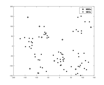
Figure 1: The two-tier HCN model with intra-tier dependence ($\lambda_{m}=$0.0001, $\lambda_{p}=0.0002$, $c$=4, $R=30$)

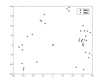
Figure 2: The two-tier HCN model with both inter-tier and intra-tier dependence ($\lambda_{0}=0.00001,$ $c_{1}=10$, $D_{1}=200$, $c_{2}=3$, $D_{2}=25$)

II System Model

We consider a two-tier HCN consisting of macrocell BSs (MBSs) and small cell BSs (SBSs). Regarding the dependence among the BSs in HCNs, MBSs and SBSs are respectively modeled as a homogenous PPP and a non-Poisson point process, which is shown in the sequel. MBSs and SBSs transmit at fixed power $P{}_{tm}$ and $P{}_{ts}$, respectively. The power received by the user located at $u$ from BS $x$ in time slot $t$ is expressed as $P_{t}h_{xu}\left(t\right)g\left(x-u\right)$, where $P_{t}$ is $P_{tm}$ or $P_{ts}$ based on the type of BS, $h_{xu}\left(t\right)$ denotes the temporally and spatially independent small-scale fading, and $g\left(x\right)$ represents the large-scale path loss.

II-A Two-tier HCNs Model with Intra-tier Dependence (Case 1)

In view of intra-tier dependence, SBSs are independently clustered in Case 1. As shown in Fig. 1, MBSs and SBSs are distributed as a PPP $\phi_{m}=\{x_{1},x_{2},\cdots\}\subset\mathbb{R}^{2}$ with density $\lambda_{m}$ and an independent MCP $\phi_{s}=\left\{y_{1},y_{2},\cdots\right\}\subset\mathbb{R}^{2}$ whose parent point process is an independent PPP with density $\lambda_{p}$. To be specific, the number of SBSs in each cluster is a Poisson random variable with mean $c$. In addition, each SBS is uniformly scattered in a ball of radius $R$ around its parent point. Thus, the probability density function (pdf) of the typical cluster whose parent point located at origin is expressed as

$$f_{cl}\left(y\right)=\begin{cases}\frac{1}{\pi R^{2}},&\parallel y\parallel\leq R\\ 0,&otherwise.\end{cases}$$ (1)

II-B Two-tier HCNs Model with both Inter-tier and Intra-tier Dependence (Case 2)

As illustrated in Fig. 2, SBSs in Case 2 are clustered in the edge region of macrocell due to the inter-tier dependence. In Case 2, MBSs follow a PPP $\phi_{m}=\{x_{1},x_{2},\cdots\}\subset\mathbb{R}^{2}$ with density $\lambda_{m}$ and SBSs follow a SOCP $\phi_{s}=\left\{z_{1},z_{2},\cdots\right\}\subset\mathbb{R}^{2}$ whose parent process is a PPP with density $\lambda_{0}$. These parent points denote the centers of first-order clusters in which the number of points is Poisson random variable with mean $c_{1}$. It is worth noting that in Case 2, MBSs are the parent points of SBSs following SOCP because of the inter-tier dependence. Thus, $\lambda_{0}=\lambda_{m}$. Moreover, each point of a first-order cluster is isotropically scattered according to a centered reverse Gaussian distribution. Thus, the pdf of first-order cluster point is correspondingly given as [17]:

$$f_{cl_{1}}\left(x\right)=\begin{cases}\frac{\left(1-\exp\left(\frac{-\|x\|^{2}}{2\sigma^{2}}\right)\right)}{\pi D_{1}^{2}+2\pi\sigma^{2}\left(\exp\left(\frac{-D_{1}^{2}}{2\sigma^{2}}\right)-1\right)},&\|x\|\leq D_{1}\\ 0,&otherwise,\end{cases}$$ (2)

where $D_{1}$ is the radius of the coverage area of first-order cluster and $\sigma$ denotes the standard deviation of reverse Gaussian distribution. These first-order cluster points are the centers of the second-order cluster points, i.e., SBSs, whose number is a Poisson random variable with mean $c_{2}$. Each SBS is uniformly scattered in a ball of radius $D_{2}$ around the first-order cluster points and the corresponding pdf is given by

$$f_{cl_{2}}\left(x\right)=\begin{cases}\frac{1}{\pi D_{2}^{2}},&\parallel x\parallel\leq D_{2}\\ 0,&otherwise.\end{cases}$$ (3)

III Spatio-temporal Interference Correlation

Since the interference correlation in Poisson networks has been investigated in [5], in this section, we focus on the spatio-temporal interference correlation when the interferers follow MCP and SOCP. We find that the interference correlations in Matern cluster networks and second-order cluster networks are greater than that in Poisson networks. Theorem 1 shows the expressions of these interference correlation coefficients.

Theorem 1. The spatio-temporal correlation coefficients of interference when the interferers follow MCP and SOCP are respectively:

$$\zeta_{MCP}=\frac{\int_{\mathbb{R}^{2}}g\left(x\right)g\left(x-\parallel u-v\parallel\right)\mathrm{d}x+F\left(c,R\right)}{\frac{\mathbb{E}\left[h^{2}\right]}{\mathbb{E}\left[h\right]^{2}}\int_{\mathbb{R}^{2}}g^{2}\left(x\right)\mathrm{d}x+F\left(c,R\right)},$$ (4)

and

$$\zeta_{SOCP}=\frac{\int_{\mathbb{R}^{2}}g\left(x\right)g\left(x-\parallel u-v\parallel\right)\mathrm{d}x+F\left(c_{2},D_{2}\right)}{\frac{\mathbb{E}\left[h^{2}\right]}{\mathbb{E}\left[h\right]^{2}}\int_{\mathbb{R}^{2}}g^{2}\left(x\right)\mathrm{d}x+F\left(c_{2},D_{2}\right)},$$ (5)

where $F\left(c,R\right)=\frac{c}{\pi^{2}R^{4}}\int_{\mathbb{R}^{2}}\int_{\mathbb{R}^{2}}g\left(x\right)g\left(y\right)A_{R}\left(\|x-y\|\right)\mathrm{d}x\mathrm{d}y$, and $A_{R}\left(r\right)=2R^{2}\mathcal{\arccos}\left(\frac{r}{2R}\right)-r\sqrt{R^{2}-\frac{r^{2}}{4}},\;0\leq r\leq 2R$, and 0 for $r>2R$.

Proof:

See Appendix A. ∎

To better understand the proof, we now give a brief introduction of the main steps. We calculate the correlation coefficient of interference according to its definition. Specifically, we first calculate the mean of interference $I_{t}\left(u\right)$, the mean product of $I_{t_{1}}\left(u\right)$ and $I_{t_{2}}\left(v\right)$, and the second moment of the interference $I_{t}\left(u\right)$. Then, we substitute the corresponding results into the definition of interference correlation coefficient to get the expression.

Recall that the interference correlation coefficient in Poisson networks is given in [5] as

$$\zeta_{PPP}=\frac{\int_{\mathbb{R}^{2}}g\left(x\right)g\left(x-\parallel u-v\parallel\right)\mathrm{d}x}{\frac{\mathbb{E}\left[h^{2}\right]}{\mathbb{E}\left[h\right]^{2}}\int_{\mathbb{R}^{2}}g^{2}\left(x\right)\mathrm{d}x}.$$ (6)

Comparing $\zeta_{MCP}$ and $\zeta_{SOCP}$ with $\zeta_{PPP}$, the function $F\left(c,R\right)$ captures the contribution of clustering in interferers on interference correlation, which depends on the mean number of points and the radius of each cluster.

Remark 1. The interference correlation coefficient under MCP distributed interferers is the same with that under SOCP distributed interferers if they have the same average number of points and the radius for each cluster, i.e., $\zeta_{MCP}=\zeta_{SOCP}$ if $c=c_{2}$ and $R=D_{2}$. The fact is intuitive because the contribution of the clustering in interference correlation $F\left(c,R\right)$ is only decided by $c$ and $R$. Further, we give the relationship between the interference correlation coefficients under MCP or SOCP distributed interferers and that under PPP distributed interferers in Proposition 1.

Proposition 1. The interference correlation coefficients $\zeta_{MCP}$ and $\zeta_{SOCP}$ are greater than that in Poisson networks $\zeta_{PPP}$, i.e., $\zeta_{MCP}>\zeta_{PPP}$ and $\zeta_{SOCP}>\zeta_{PPP}$.

Proof:

For simplicity, we denote $P=\int_{\mathbb{R}^{2}}g\left(x\right)g\left(x-\parallel u-v\parallel\right)\mathrm{d}x$, $Q=\frac{\mathbb{E}\left[h^{2}\right]}{\mathbb{E}\left[h\right]^{2}}\int_{\mathbb{R}^{2}}g^{2}\left(x\right)\mathrm{d}x$. In this way, $\zeta_{PPP}$, $\zeta_{MCP}$, and $\zeta_{SOCP}$ are simplified to $\zeta_{PPP}=\frac{P}{Q}$, where $P>0$ and $Q>0$, $\zeta_{MCP}=\frac{P+F\left(c,R\right)}{Q+F\left(c,R\right)}$, and $\zeta_{SOCP}=\frac{P+F\left(c_{2},D_{2}\right)}{Q+F\left(c_{2},D_{2}\right)}$. Now, we show that $\zeta_{MCP}>\zeta_{PPP}$.

$$\zeta_{MCP}-\zeta_{PPP}=\frac{P+F\left(c,R\right)}{Q+F\left(c,R\right)}-\frac{P}{Q}$$

$$=\frac{\left(Q-P\right)F\left(c,R\right)}{Q\left(Q+F\left(c,R\right)\right)}\overset{\left(a\right)}{>0},$$ (7)

where $(a)$ comes from the fact that $F\left(c,R\right)>0$ and $Q-P>0$ (since $0<\zeta_{PPP}<1$).

Following the similar steps, we can get $\zeta_{SOCP}>\zeta_{PPP}$. ∎

From Proposition 1, we find that the spatial correlation in interferers significantly affects the correlation in interference. In particular, the attraction between the interferers enhances the correlation in interference. Thus, we infer that reducing the clustering in interferers enables weaken the interference correlation. Next, we study the effect of system parameters, such as $c$ and $R$, on the interference correlation.

Proposition 2. The interference correlation coefficients $\zeta_{MCP}$ and $\zeta_{SOCP}$ increase with the increase in $c$ or $c_{2}$, while decrease with the increase in $R$ or $D_{2}$. In particular, $\zeta_{MCP}\rightarrow\zeta_{PPP}$, if $\frac{c}{\pi^{2}R^{2}}\rightarrow 0$ and $\zeta_{SOCP}\rightarrow\zeta_{PPP}$, if $\frac{c_{2}}{\pi^{2}D_{2}^{2}}\rightarrow 0$.

Proof:

Recall that the interference correlation coefficient $\zeta_{MCP}$ can be denoted as $\zeta_{MCP}=\frac{P+F}{Q+F}$. Taking the derivative of $\zeta_{MCP}$ with respect to $F$, we get $\zeta^{\prime}_{MCP}=\frac{Q-P}{\left(Q+P\right)^{2}}$. It should be noted that $0<\zeta_{PPP}=\frac{P}{Q}<1$. Thus, $\zeta^{\prime}_{MCP}>0$, i.e., $\zeta_{MCP}$ increases with the increase in $F$. Moreover, from the expression of $F\left(c,R\right)$, we know that $F\left(c,R\right)\propto c$ and $F\left(c,R\right)\propto\frac{1}{R^{2}}$. As a result, $\zeta_{MCP}$ increases as $c$ increases, while it decreases as $R$ increases.

In addition, $F\left(c,R\right)\rightarrow 0$, if $\frac{c}{\pi^{2}R^{2}}\rightarrow 0$. Thus, $\zeta_{MCP}\rightarrow\zeta_{PPP}$, if $\frac{c}{\pi^{2}R^{2}}\rightarrow 0$.

The same conclusion for $\zeta_{SOCP}\left(I_{t_{1}}\left(u\right),I_{t_{2}}\left(v\right)\right)$ can be obtained via following the similar steps. ∎

The conclusion in Proposition 2 can be explained as follows. Given $R$ or $D_{2}$, the larger $c$ or $c_{2}$ is, the more attraction the interferers has. Moreover, the attraction of the interferers has a positive effect on interference correlation. As a result, the correlation coefficient increases with the increase in $c$ or $c_{2}$. Similarly, the correlation coefficient increases with the decrease in $R$ or $D_{2}$, since the attraction among the interferers becomes strong when $R$ or $D_{2}$ decreases.

When $\frac{c}{\pi^{2}R^{2}}\rightarrow 0$, the effect of clustering in interferers can be ignored. In particular, when the radius of cluster $R$ or $D_{2}$ approximates to infinity, MCP and SOCP can be viewed as the superposition of finite independent PPP. Thus, $\zeta_{MCP}\rightarrow\zeta_{PPP},\>R\rightarrow\infty$ and $\zeta_{SOCP}\rightarrow\zeta_{PPP},\>D_{2}\rightarrow\infty$, since the summation of multiple independent PPP is also a PPP.

Figure 3: Interference correlation coefficient with different $\epsilon$ ($\alpha=4$, $P=43$dBm, $\lambda_{p}=0.01,$ $c=3$, $R=1$)

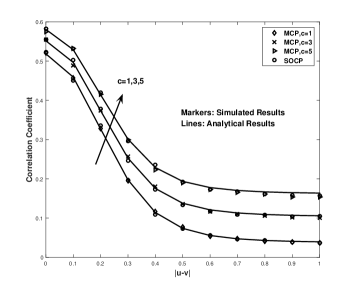
Figure 4: Interference correlation coefficient with different $c$ ($\alpha=4$, $P=43$dBm, $\lambda_{0}=\lambda_{p}=0.01,$ $c_{1}=10$, $D_{1}=10$, $c_{2}=c$, $D_{2}=R=1$, $\sigma=3$, $\epsilon=0.00001$)

IV Performance Analysis

In this section, Monte Carlo simulations are conducted to validate the analysis of interference correlation coefficients. Further, we show the impact of the average number of points and the radius of each cluster on the interference correlation. In the simulation, the interferers follow PPP, MCP, and SOCP. For comparing the interference correlation coefficients under different distributed interferers, we set the densities of interferers as $\lambda_{PPP}=\lambda_{p}c=\lambda_{0}c_{1}c_{2}$.

Fig. 3 compares the interference correlation coefficient in the case of the interferers following MCP and PPP. The lines and dotted lines represent the analytical results for MCP and PPP, respectively, while the markers are the corresponding simulated results. First, our results in Theorem 1 are validated as the simulated results match well with the analytical results. In addition, we find that the correlation of interference in MCP is greater than that in PPP. It shows that the spatial correlation in interferers has a significant effect on interference correlation. Specifically, the attraction among the interferers enhances the interference correlation. Moreover, as the distance between the tested points grows, the interference correlation coefficient decreases, which is coincide with our intuition. The farther the two points are, the less interference correlation they have.

Fig. 4 illustrates the interference correlation coefficients under different mean numbers of points in each cluster. Note that we only show the analytical interference correlation coefficient for the interferers following MCP. This is because, according to our analysis (Remark 1), the interference correlation coefficient under SOCP is the same as that under MCP when $c=c_{2}$ and $D_{2}=R$. From Fig. 4, we find that the interference correlation coefficient is improved with the increase in the mean number of points in each cluster. The reason is that the clustering in interferers exacerbates the interference correlation. Given the radius of each cluster, increasing the average number of each cluster aggravates the clustering in interferers. Thus, increasing the mean number of points in each cluster enhances the correlation in interference.

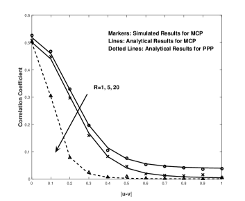
Figure 5: Interference correlation coefficient with different $R$ ($\alpha=4$, $P=43$dBm, $\lambda_{0}=\lambda_{p}=0.01,$ $c_{1}=10$, $D_{1}=10$, $c_{2}=c=1$, $D_{2}=R$, $\sigma=3$, $\epsilon=0.001$)

Fig. 5 shows the interference correlation coefficients varying with different radiuses of each cluster. It is shown that the interference correlation coefficient decreases with the increase in the radius of each cluster $R$. The reason is that, given the average number of each cluster, the larger the radius is, the less clustering impact is. As a result, the interference correlation coefficient decreases. In particular, the interference correlation coefficients under MCP and SOCP approximate to that under PPP when $R=20$. This is because when $R=20$ and $c=1$, $\frac{c}{\pi R^{2}}\rightarrow 0$. Based on the conclusion in Proposition 2, the impact of clustering on the interference correlation can be ignored in this case.

V Conclusions

In this paper, we have quantified the interference correlation in non-Poisson networks including Matern cluster networks and second-order cluster networks. It is shown that both the interference correlation coefficients are greater than that in Poisson networks, i.e., $\zeta_{MCP}>\zeta_{PPP}$ and $\zeta_{SOCP}>\zeta_{PPP}$. This indicates the clustering in MCP and SOCP has a positive contribution on the interference correlation. Moreover, we have proved that the decrease of the mean number of points in each cluster $c$ or the increase in the radius of each cluster $R$ mitigates the interference correlation. In particular, we have pointed that the effect of clustering on interference correlation can be ignored under the condition that $\frac{c}{\pi^{2}R^{2}}\rightarrow 0$.

The used methodology and achieved results clear the way to analyze the interference correlation in non-Poisson networks. A follow-up topic is to investigate the interference correlation in other non-Poisson networks. In addition, the analysis in this paper can be extended to the performance analysis of HCNs with dependence.

VI Appendix: Proofs

VI-A Proof of Theorem 1

Proof:

First, we derive the correlation coefficient when the interference comes from the BSs following MCP. In this case, the interference at a randomly chosen user $u$ at time slot $t$ is given as

$$I_{t}\left(u\right) =\sum_{x\in\phi_{MCP}}P_{t}h_{xu}\left(t\right)g\left(x-u\right)$$

$$=\sum_{y\in\phi_{p}}\sum_{x\in\phi^{\left[y\right]}}P_{t}h_{xu}\left(t\right)g\left(x-u\right),$$ (8)

where $\phi_{p}$ represents the parent process of MCP and $\phi^{\left[y\right]}$ denotes the cluster associated with parent point $y\in\phi_{p}$.

The mean interference is given by

$$\mathbb{E}\left[I_{t}\left(u\right)\right]$$

$$=\mathbb{E}\left[\sum_{y\in\phi_{p}}\sum_{x\in\phi^{\left[y\right]}}P_{t}h_{xu}\left(t\right)g\left(x-u\right)\right]$$

$$\overset{\left(a\right)}{=}P_{t}\mathbb{E}\left[h\right]\lambda_{p}\int_{\mathbb{R}^{2}}\mathbb{E}\left[\sum_{x\in\phi^{\left[y\right]}}g\left(x-u\right)\right]\mathrm{d}y$$

$$\overset{\left(b\right)}{=}P_{t}\mathbb{E}\left[h\right]\lambda_{p}c\int_{\mathbb{R}^{2}}\int_{\mathbb{R}^{2}}g\left(x-u-y\right)f_{cl}\left(x\right)\mathrm{d}x\mathrm{d}y$$

$$=P_{t}\mathbb{E}\left[h\right]\lambda_{p}c\int_{\mathbb{R}^{2}}g\left(x-u\right)\int_{\mathbb{R}^{2}}f_{cl}\left(x+y\right)\mathrm{d}y\mathrm{d}x$$

$$\overset{\left(c\right)}{=}P_{t}\mathbb{E}\left[h\right]\lambda_{p}c\int_{\mathbb{R}^{2}}g\left(x\right)\mathrm{d}x,$$ (9)

where $\left(a\right)$ and $\left(b\right)$ come from Campbell-Mecke Theorem, $\left(c\right)$ follows the fact that $\int_{\mathbb{R}^{2}}f_{cl}\left(x\right)\mathrm{d}x=1$.

The mean product of $I_{t_{1}}\left(u\right)$ and $I_{t_{2}}\left(v\right)$ is given by

$$\mathbb{E}\left[I_{t_{1}}\left(u\right),I_{t_{2}}\left(v\right)\right]$$

$$=\mathbb{E}\left[\sum_{x\in\phi_{MCP}}\!\!\!\!\!P_{t}h_{xu}\left(t_{1}\right)g\left(x-u\right)\sum_{y\in\phi_{MCP}}\!\!\!\!\!P_{t}h_{yv}\left(t_{2}\right)g\left(y-v\right)\right]$$

$$=\mathbb{E}\left[\sum_{x\in\phi_{MCP}}P_{t}^{2}h_{xu}\left(t_{1}\right)h_{xv}\left(t_{2}\right)g\left(x-u\right)g\left(x-v\right)\right]$$

$$+\mathbb{E}\left[\sum_{x,y\in\phi_{MCP}}^{x\neq y}P_{t}^{2}h_{xu}\left(t_{1}\right)h_{yv}\left(t_{2}\right)g\left(x-u\right)g\left(y-v\right)\right].$$ (10)

Let

$$F=\mathbb{E}\left[\sum_{x\in\phi_{MCP}}P_{t}^{2}h_{xu}\left(t_{1}\right)h_{xv}\left(t_{2}\right)g\left(x-u\right)g\left(x-v\right)\right],$$

and

$$Q=\mathbb{E}\left[\sum_{x,y\in\phi_{MCP}}^{x\neq y}P_{t}^{2}h_{xu}\left(t_{1}\right)h_{yv}\left(t_{2}\right)g\left(x-u\right)g\left(y-v\right)\right].$$

Next, we calculate $F$ and $Q$, respectively.

$$F =\mathbb{E}\left[\sum_{x\in\phi_{MCP}}P_{t}^{2}h_{xu}\left(t_{1}\right)h_{xv}\left(t_{2}\right)g\left(x-u\right)g\left(x-v\right)\right]$$

$$=P_{t}^{2}\mathbb{E}\left[h\right]^{2}\mathbb{E}\left[\sum_{y\in\phi_{p}}\sum_{x\in\phi^{\left[y\right]}}g\left(x-u\right)g\left(x-v\right)\right]$$

$$\overset{\left(a\right)}{=}P_{t}^{2}\mathbb{E}\left[h\right]^{2}\lambda_{p}c\int_{\mathbb{R}^{2}}g\left(x-u\right)g\left(x-v\right)\mathrm{d}x,$$ (11)

where $\left(a\right)$ comes from Campbell-Mecke Theorem and the fact that $\int_{\mathbb{R}^{2}}f_{cl}\left(x\right)\mathrm{d}x=1$.

$$Q =\mathbb{E}\left[\sum_{x,y\in\phi_{MCP}}^{x\neq y}P_{t}^{2}h_{xu}\left(t_{1}\right)h_{yv}\left(t_{2}\right)g\left(x-u\right)g\left(y-v\right)\right]$$

$$=P_{t}^{2}\mathbb{E}\left[h\right]^{2}\mathbb{E}\left[\sum_{x,y\in\phi_{MCP}}^{x\neq y}g\left(x-u\right)g\left(y-v\right)\right]$$

$$\overset{\left(a\right)}{=}P_{t}^{2}\mathbb{E}\left[h\right]^{2}\int_{\mathbb{R}^{2}}\int_{\mathbb{R}^{2}}g\left(x\right)g\left(y\right)\rho_{MCP}^{\left(2\right)}\left(x,y\right)\mathrm{d}x\mathrm{d}y$$

$$\overset{\left(b\right)}{=}P_{t}^{2}\mathbb{E}\left[h\right]^{2}\left(\lambda_{p}c\right)^{2}\int_{\mathbb{R}^{2}}\int_{\mathbb{R}^{2}}g\left(x\right)g\left(y\right)\mathrm{d}x\mathrm{d}y$$

$$+P_{t}^{2}\mathbb{E}\left[h\right]^{2}\lambda_{p}c\cdot F\left(c,R\right),$$ (12)

where $\left(a\right)$ follows from $x=x-u$, $y=y-v$, $\left(b\right)$ comes from the second moment density of MCP given by [18, p. 128], $F\left(c,R\right)=\frac{c}{\pi^{2}R^{4}}\int_{\mathbb{R}^{2}}\int_{\mathbb{R}^{2}}g\left(x\right)g\left(y\right)A_{R}\left(\|x-y\|\right)\mathrm{d}x\mathrm{d}y$, and $A_{R}\left(r\right)=2R^{2}\mathcal{\arccos}\left(\frac{r}{2R}\right)-r\sqrt{R^{2}-\frac{r^{2}}{4}},\;0\leq r\leq 2R$, and 0 for $r>2R$. Substituting (11) and (12) into (10), we get the mean product of $I_{t_{1}}\left(u\right)$ and $I_{t_{2}}\left(v\right)$

$$\mathbb{E}\left[I_{t_{1}}\left(u\right),I_{t_{2}}\left(v\right)\right] =P_{t}^{2}\mathbb{E}\left[h\right]^{2}\lambda_{p}c\int_{\mathbb{R}^{2}}g\left(x-u\right)g\left(x-v\right)\mathrm{d}x$$

$$+P_{t}^{2}\mathbb{E}\left[h\right]^{2}\left(\lambda_{p}c\right)^{2}\int_{\mathbb{R}^{2}}\int_{\mathbb{R}^{2}}g\left(x\right)g\left(y\right)\mathrm{d}x\mathrm{d}y$$

$$+P_{t}^{2}\mathbb{E}\left[h\right]^{2}\lambda_{p}c\cdot F\left(c,R\right),$$ (13)

Similarly, the second moment of interference is given as

$$\mathbb{E}\left[I_{t}^{2}\left(u\right)\right]$$

$$=P_{t}^{2}\mathbb{E}\left[h^{2}\right]\lambda_{p}c\int_{\mathbb{R}^{2}}g^{2}\left(x\right)\mathrm{d}x$$

$$+P_{t}^{2}\mathbb{E}\left[h\right]^{2}\left(\lambda_{p}c\right)^{2}\int_{\mathbb{R}^{2}}\int_{\mathbb{R}^{2}}g\left(x-u\right)g\left(y-v\right)\mathrm{d}x\mathrm{d}y$$

$$+P_{t}^{2}\mathbb{E}\left[h\right]^{2}\lambda_{p}c\cdot F\left(c,R\right).$$ (14)

Interference correlation coefficient is defined as

$$\zeta\left(I_{t_{1}}\left(u\right),I_{t_{2}}\left(v\right)\right)=\frac{\mathbb{E}\left[I_{t_{1}}\left(u\right),I_{t_{2}}\left(v\right)\right]-\mathbb{E}\left[I_{t_{1}}\left(u\right)\right]\mathbb{E}\left[I_{t_{2}}\left(v\right)\right]}{\sqrt{var\left(I_{t_{1}}\left(u\right)\right)}\cdot\sqrt{var\left(I_{t_{2}}\left(v\right)\right)}}.$$ (15)

Substituting (9), (13), and (14) into (15), we derive the correlation coefficient of interference when the interferers following MCP.

Next, we will calculate the correlation coefficient of interference when the interferers following SOCP. The key to the calculation is to derive the second moment density of SOCP $\rho_{SOCP}^{\left(2\right)}\left(x,y\right)$. According to [18, p. 127], there are two contributions to the second moment density including the one from pairs of points in different clusters and the one from pairs of points in the same cluster. Since difference clusters in SOCP are independent, the second moment density of SOCP is expressed as

$$\rho_{SOCP}^{\left(2\right)}\left(u,v\right)=\lambda^{2}+\mathbb{E}\left[\sum_{x\in\phi_{P_{0}}}\sum_{y\in\phi_{P_{1}^{\left[x\right]}}}h\left(u,v\mid x,y\right)\right],$$ (16)

where $\lambda=\lambda_{0}c_{1}c_{2}$ denotes the intensity of SOCP, $\phi_{P_{0}}$ represents the parent process with intensity $\lambda_{0}$, $\phi_{P_{1}^{\left[x\right]}}$ is the first-order cluster associated with parent point $x\in\phi_{P_{0}}$, $h\left(u,v\mid x,y\right)$ denotes the conditional second moment density.

$$\mathbb{E}\left[\sum_{x\in\phi_{P_{0}}}\sum_{y\in\phi_{P_{1}^{\left[x\right]}}}h\left(u,v\mid x,y\right)\right]$$

$$\overset{\left(a\right)}{=} \mathbb{E}\left[\sum_{x\in\phi_{P_{0}}}\sum_{y\in\phi_{P_{1}^{\left[x\right]}}}c_{2}f_{cl_{2}}\left(u-y-x\right)c_{2}f_{cl_{2}}\left(v-y-x\right)\right]$$

$$\overset{\left(b\right)}{=} \lambda_{0}c_{1}\!\!\left(c_{2}\right)^{2}\!\!\!\int_{\mathbb{R}^{2}}\!\!\!\int_{\mathbb{R}^{2}}\!\!f_{cl_{1}}\left(y\right)\!\!f_{cl_{2}}\left(u-y-x\right)\!\!f_{cl_{2}}\left(v-y-x\right)\mathrm{d}x\mathrm{d}y$$

$$= \lambda_{0}c_{1}\left(c_{2}\right)^{2}\left(f_{cl_{2}}\star f_{cl_{2}}\right)\left(u-v\right)\int_{\mathbb{R}^{2}}f_{cl_{1}}\left(y\right)\mathrm{d}y$$

$$\overset{\left(c\right)}{=} \lambda_{0}c_{1}\left(c_{2}\right)^{2}\left(f_{cl_{2}}\star f_{cl_{2}}\right)\left(u-v\right)$$

$$\overset{\left(d\right)}{=} \lambda_{0}c_{1}\left(c_{2}\right)^{2}\cdot\frac{A_{D_{2}}\left(\|x-y\|\right)}{\pi^{2}D_{2}^{4}},$$ (17)

where $\left(a\right)$ follows from the independence of the points in the same cluster, $\left(b\right)$ comes from Campbell-Mecke Theorem, $\left(c\right)$ follows from the fact that $\int_{\mathbb{R}^{2}}f_{cl_{1}}\left(y\right)\mathrm{d}y=1$, $\left(d\right)$ comes from the calculation of $\left(f_{cl_{2}}\star f_{cl_{2}}\right)\left(u-v\right)$ which is given in [18] and $A_{D_{2}}\left(r\right)=2D_{2}^{2}\arccos\left(\frac{r}{2D_{2}}\right)-r\sqrt{D_{2}^{2}-\frac{r^{2}}{4}},\;0\leq r\leq 2D_{2}$.

Based on the derived second moment density of SOCP, we get the correlation coefficient of interference when the interferers following SOCP. ∎

References

- [1] U. Schilcher, C. Bettstetter, and G. Brandner, “Temporal correlation of interference in wireless networks with rayleigh block fading,” IEEE Trans. Mobile Comp., vol. 11, no. 12, pp. 2109–2120, Dec. 2012.
- [2] K. Gulati, R. Ganti, J. Andrews, B. Evans, and S. Srikanteswara, “Characterizing decentralized wireless networks with temporal correlation in the low outage regime,” IEEE Trans. Wireless Commun., vol. 11, no. 9, pp. 3112–3125, September 2012.
- [3] Y. Cong, X. Zhou, and R. Kennedy, “Interference prediction in mobile ad hoc networks with a general mobility model,” IEEE Trans. Wireless Commun., vol. 14, no. 8, pp. 4277–4290, Aug 2015.
- [4] R. Tanbourgi, H. S. Dhillon, J. G. Andrews, and F. K. Jondral, “Effect of spatial interference correlation on the performance of maximum ratio combining,” IEEE Trans. Wireless Commun., vol. 13, no. 6, pp. 3307–3316, June 2014.
- [5] R. Ganti and M. Haenggi, “Spatial and temporal correlation of the interference in ALOHA ad hoc networks,” IEEE Commun. Lett., vol. 13, no. 9, pp. 631–633, Sep. 2009.
- [6] M. Haenggi and R. Smarandache, “Diversity polynomials for the analysis of temporal correlations in wireless networks,” IEEE Trans. Wireless Commun., vol. 12, no. 11, pp. 5940–5951, Nov. 2013.
- [7] M. Haenggi, “Diversity loss due to interference correlation,” IEEE Commun. Lett., vol. 16, no. 10, pp. 1600–1603, Oct. 2012.
- [8] Z. Gong and M. Haenggi, “Interference and outage in mobile random networks: Expectation, distribution, and correlation,” IEEE Trans. Mobile Comp., vol. 13, no. 2, pp. 337–349, Feb. 2014.
- [9] Y. Zhong, W. Zhang, and M. Haenggi, “Managing interference correlation through random medium access,” IEEE Trans. Wireless Commun., vol. 13, no. 2, pp. 928–941, Feb. 2014.
- [10] J. Wen, M. Sheng, B. Liang, X. Wang, Y. Zhang, and J. Li, “Correlations of interference and link successes in heterogeneous cellular networks,” in Proc. IEEE GLOBECOM, San Diego, CA, USA, Dec. 2015.
- [11] M. Sheng, J. Wen, J. Li, and B. Liang, “Correlations of interference and link successes in heterogeneous cellular networks,” submitted to IEEE Trans. Wireless Commun., 2014, available at http://arxiv.org/abs/1411.4781.
- [12] I. Hwang, B. Song, and S. Soliman, “A holistic view on hyper-dense heterogeneous and small cell networks,” IEEE Comm. Mag., vol. 51, no. 6, pp. 20–27, Jun. 2013.
- [13] J. Weitzen, L. Mingzhe, E. Anderland, and V. Eyuboglu, “Large-scale deployment of residential small cells,” Proc. IEEE, vol. 101, no. 11, pp. 2367–2380, Nov. 2013.
- [14] R. Ganti and M. Haenggi, “Interference and outage in clustered wireless ad hoc networks,” IEEE Trans. Inf. Theory, vol. 55, no. 9, pp. 4067–4086, Sept 2009.
- [15] J. Young, M. Hasna, and A. Ghrayeb, “Modeling heterogeneous cellular networks interference using poisson cluster processes,” IEEE J. Sel. Areas Commun., vol. 33, no. 10, pp. 2182–2195, Oct. 2015.
- [16] N. Deng, W. Zhou, and M. Haenggi, “Heterogeneous cellular network models with dependence,” IEEE J. Sel. Areas Commun., vol. 33, no. 10, pp. 2167–2181, Oct. 2015.
- [17] S. Asif and K. Kwak, “Downlink coverage and rate analysis of two-tier networks,” IEEE Wireless Comms. Lett., vol. 4, no. 2, pp. 133–136, Apr. 2015.
- [18] M. Haenggi, Stochastic Geometry for Wireless Networks. Cambridge University Press, 2012.