Latent Model Ensemble with Auto-localization

Abstract

Deep Convolutional Neural Networks (CNN) have exhibited superior performance in many visual recognition tasks including image classification, object detection, and scene labeling, due to their large learning capacity and resistance to overfit. For the image classification task, most of the current deep CNN-based approaches take the whole size-normalized image as input and have achieved quite promising results. Compared with the previously dominating approaches based on feature extraction, pooling, and classification, the deep CNN-based approaches mainly rely on the learning capability of deep CNN to achieve superior results: the burden of minimizing intra-class variation while maximizing inter-class difference is entirely dependent on the implicit feature learning component of deep CNN; we rely upon the implicitly learned filters and pooling component to select the discriminative regions, which correspond to the activated neurons. However, if the irrelevant regions constitute a large portion of the image of interest, the classification performance of the deep CNN, which takes the whole image as input, can be heavily affected. To solve this issue, we propose a novel latent CNN framework, which treats the most discriminate region as a latent variable. We can jointly learn the global CNN with the latent CNN to avoid the aforementioned big irrelevant region issue, and our experimental results show the evident advantage of the proposed latent CNN over traditional deep CNN: latent CNN outperforms the state-of-the-art performance of deep CNN on standard benchmark datasets including the CIFAR-10, CIFAR-100, MNIST and PASCAL VOC 2007 Classification dataset.

I Introduction

The last decade of progress on various visual recognition tasks has for the most part been based on the use of SIFT [1] and HOG [2]. The recent success of CNNs is attributed to their ability to learn rich mid-level image representations as opposed to hand-designed low-level features used in other image classification methods.  [3] has demonstrated that deep CNN features are substantially different from and complementary to those traditional features used in object detection. Searching the parameter space of deep architectures is a difficult task because the training criterion is non-convex and involves many local minima. Nevertheless, deep architecture is capable of automatically learning and fusing rich hierarchical features in an integrated framework. Many techniques, such as Relu [4], Dropout [5], Dropconnect [6], pre-training [7] and data augmentation [8], have been proposed to enhance the performance of deep architectures. Though learning CNN will get into local minima or in a plateau (where due to low curvature the gradients become extremely small), deep convolutional neural networks recently achieved remarkable success in many visual recognition tasks, such as image classification and object detection, fine-grained recognition, and visual instance retrieval [9]. For the image classification task, most of the current deep CNN-based approaches take the whole size-normalized image for input. However, it is very likely that the region of interest in the image may just take a small portion of the image of interest, especially for the object classification task of PASCAL VOC dataset. Figure 1 shows some images from the PASCAL VOC 2007 classification dataset  [10]. Figure 1(a) is a perfect example for whole image input data, which is centered and occupies a large portion of the image. However, Figure 1(b), which is labeled ”potted plant”, would make the learning more complicated for CNN’s use of the whole image as input. The most challenge is that Figure 1(c) has multiple labels. Currently supervised learning CNN takes (data, label) pairs as input; Hence, multiple labeled images would tend to confuse the CNN model.

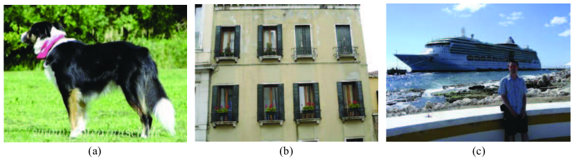
Figure 1: Some PASCAL VOC 2007 images. Irrelated regions increase the complexity of CNN learning, which is especially evident in Fig. 1(b) and (c). Figure (a) (b) are labeled as dog and potted plant respectively. Figure (c) has two labels: boat and person.

In order to reduce the effect of irrelated regions, we propose a novel framework called latent CNN, which would select the most discriminating region as input for deep CNNs. In this view, latent CNN could also be seen as region-level CNN instead of traditional image-level CNN, which takes the whole size-normalized image as input.

One straightforward way to reduce the effect of local minima is to make full use of multiple CNNs with different random initialization [4]. Given multiple CNNs, people simply use majority voting or average the confidence scores from different CNNs. The second contribution in our paper is that we propose a new combination scheme called Latent Model Ensemble, which outperforms the state-of-the-art performance on CIFAR-10 [11], CIFAR-100 [11], MNIST [12], and PASCAL VOC 2007 Classification dataset [10].

In summary, this paper introduces the following contributions: (i) a latent CNN framework, which automatically selects the most discriminate region to reduce the effect of irrelevant regions, (ii) a new combination scheme for multiple CNNs via Latent Model Ensemble, and (iii) state-of-the-art performance on CIFAR-10 [11], CIFAR-100 [11], MNIST [12] and PASCAL VOC 2007 Classification dataset [10].

II Latent CNN Framework

Latent CNN contains two key components: deep CNN structures and latent SVM, which we will present in detail in Sections  II-A and  II-B, respectively. Then we will discuss the overall latent CNN framework in  II-C.

II-A Deep CNNs

AlexNet [4] is a stack of convolutional layers, which are optionally followed by contrast normalization layers and max-pooling layers, and locally-connected layers or fully-connected layers. Transfer learning is adopted when the AlexNet is used for other smaller dataset. For example, the PASCAL VOC 2007 classification dataset [10] has only 5,011 training images, which makes it almost impossible to learn a satisfied deep CNN model.

Our CNN structure trained on ImageNet is similar to  [4], which has five convolutional layers, two fully connected layers, and one output layer. The max-pooling layers are added to conv1, conv2, and conv5 layer, respectively. The difference is that  [4] normalized all the images into 256 x 256 squares and take 224 x 224 patches as the input for the CNN structure. Our CNN structure, however, does not need to normalize the original images and it takes 128x128 patches. Compared to the AlexNet image translation method, our method may not be label-preserving transformations [13, 8, 14, 15], considering that a much smaller region probably does not satisfy the 50% overlap rule. But it is not a problem when it is applied to the latent CNN framework, which would select the most discriminative region as the input for CNN learning procedure.

Transfer learning is used for training the CNN structure for the PASCAL VOC datasets. Compared to the CNN model trained from ImageNet, it removes the last 1000-node output layer and add two more fully connected layers. During the training for the PASCAL VOC 2007 classification dataset, all the transferred parameters are fixed first and only the parameters in the last two fully connected layers are updated. Finally, a fine tuning of the whole CNN structure is applied.

II-B Multi-class Latent SVM

Before formulating the multi-class latent SVM, let’s first see the classical SVM [16]:

Assume we are given (label, feature-vector) pairs of training data $(y_{i},\mathbf{x_{i}}),i=1,...,n$. Linear classification involves the following optimization problem

$$\min_{\mathbf{w}}f(\mathbf{w})\text{, where }f(\mathbf{w})=\frac{1}{2}\mathbf{w}^{T}\mathbf{w}+C\sum_{i=1}^{n}\xi(\mathbf{w};\mathbf{x_{i}},y_{i}),$$ (1)

where $\xi(\mathbf{w};\mathbf{x_{i}},y_{i})$ is the loss function, and C is a penalty parameter. Common loss functions include

$$\xi(\mathbf{w};\mathbf{x_{i}},y_{i})=max(0,1-y_{i}\mathbf{w}^{T}\mathbf{x_{i}}),$$ (2)

$$\xi(\mathbf{w};\mathbf{x_{i}},y_{i})=max(0,1-y_{i}\mathbf{w}^{T}\mathbf{x_{i}})^{2}.$$ (3)

In analogy to classical SVMs , the latent SVM can be formulated as

$$\begin{split}&\quad\min_{\mathbf{w}}f(\mathbf{w})\text{, where }f(\mathbf{w})=\\ &\quad\frac{1}{2}tr(\mathbf{w}^{T}\mathbf{w})+C\sum_{i=1}^{n}min_{z\in Z(\mathbf{x_{i}})}(\xi(\mathbf{w};\mathbf{x_{i}},y_{i},Z)),\end{split}$$ (4)

We propose a Stochastic Gradient Descent version of latent SVM with L2 loss function , which is summarized in Algorithm 1. Notice that Algorithm 1 is a multi-class latent SVM. Model parameter matrix $\mathbf{w}$ is $FL$ x $NC$ matrix, where $FL$ is the feature length for $\Phi(\mathbf{x_{i}},z)$, and $NC$ is the number of categories. Label $y(\mathbf{x_{i}})$ is written into a $NC$ dimensional vector format in order for matrix multiplication.

Algorithm 1 SGD version of Multi-class Latent SVM

  Input: Feature vector $\Phi(\mathbf{x_{i}},Z)$, $i=1...n$, $Z$ is the latent variable space, label vector $y(\mathbf{x_{i}})$, epoch numbers $EN$, penalty parameter $C$, learning rate $lr$

  Input: Model parameter matrix $\mathbf{w}$

  $t=1$ , $t$ is the gradient update times

  for $j=1$ to $EN$ do

     for $i=1$ to $n$ do

        1. The L2 Loss is $\xi(\mathbf{w};\mathbf{x_{i}},y_{i},z)$,

        2. Find the $z_{max}$ which will maximize $\xi$ and the correspond L2 loss is $\xi_{max}$,

        3. The objective function loss is $\frac{1}{2}\mathbf{w}^{T}\mathbf{w}+C\xi_{max}$,

        4. The model parameter update gradient is $G=\mathbf{w}-2C\Phi(\mathbf{x_{i}},z_{max})\xi_{max}y(\mathbf{x_{i}},z_{max})$,

        5. Then we update the model vector $\mathbf{w}=\mathbf{w}-G/(t+T)*lr$, where $T$ is a very large fixed number

        6. $t=t+1$.

     end for

  end for

II-C Latent CNN Framework

In Figure 2, the latent CNN framework consists of a deep CNN representation stage and latent SVM selecting region stage. Given one image, the deep CNN representation stage treats all the random selected regions as input. Then the latent SVM takes those deep CNN features and selects the most discriminating region. And the selected region is used to update the parameters in the deep CNN structure.

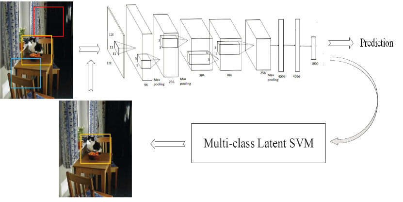
Figure 2: Latent CNN framework. The red, yellow and blue rectangular boxes are randomly selected regions. After the deep CNN representation stage and latent SVM selecting stage, only the yellow region is used to update the CNN structure.

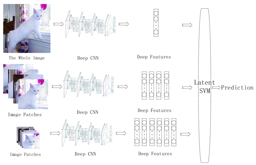
Figure 3: Latent Model Ensemble with Deep Features. The CNN in the first row is trained with the whole image, and the CNN in the second row is trained with the image patches. The latent SVM is used to select the max response from a group of patches, which is used to combine with the deep features in the first row as in Algorithm 2.

Felzenszwalb et al. [17] generalized SVMs for handling latent variables such as part positions, which is called Latent SVM (LSVM). They also proved that a latent SVM, like a hidden CRF [18], leads to a non-convex training problem. However, unlike a hidden CRF, a latent SVM is semi-convex and the training problem becomes convex once latent information is specified for the positive training examples.

For a detector with a single component in  [17], the model is defined by a coarse root filter, several higher resolution part filters and a spatial model for the location of each part relative to the root. The latent SVM is developed to train the filters and the relationship between them.

Inspired by [17], the deep CNN features extracted from the whole image are considered as the features for the ’root’ models and those features from part of the image are considered as the features for ’part’ models. In this view, our algorithm can be summarized in Algorithm 2 and the framework is illustrated in Figure 3.

II-D Latent Model Ensemble

One straightforward way to reduce the effect of local minima is to make full use of multiple CNNs with different random initializations [4]. Given multiple CNNs, people simply use majority voting or average the confidence scores from different CNNs. Latent Model Ensemble is developed based on Latent SVM[17]. Algorithm 2 is the detailed description for Latent Model Ensemble. We define the CNN trained on the whole image as root model and the CNN trained on patches of images as part model. The usage of latent SVM in Algorithm 2 has two aspect: one is used for choosing the most discrimating patch, which is used to update the latent CNN framework as shown in Figure 2, while the other is for selecting proper weight of root features and part features.

Algorithm 2 Latent Model Ensemble

  Input: Feature vector $\Phi(\mathbf{x_{i}},Z)$, $i=1...n$, $Z$ is the latent variable space, label vector $y(\mathbf{x_{i}})$, epoch numbers $EN$, penalty parameter $C$, learning rate $lr$

  Input: Model parameter matrix $\mathbf{w}$

  for $j=1$ to $EN$ do

     for $i=1$ to $n$ do

        1. Crop image into patches, and extract deep features from each patch

        2. Update the part model according to step1-step5 in the inner loop of Algorithm 1

        3. Extract deep features from the whole image

        4. Update the root model according to Equations (1) and (3).

     end for

  end for

III Experiments

We evaluate our framework based on four benchmark datasets: CIFAR-10  [11], CIFAR-100  [11], MNIST [12], and PASCAL VOC 2007 Classification dataset  [10]. To extract deep features, we use Network In Network (NIN) [19] for the first three datasets and AlexNet [4] for the PASCAL dataset. For all the datasets we use 10 part locations, designated as top left, top right, center, down left, down right, and the horizontal flip.

PASCAL VOC2007 datasets have 20 categories and contain 9,963 images. This dataset is divided into train, validation, and test subsets, which contains 2,501, 2,510 and 4,952 images, respectively. The datasets are extremely challenging since the objects vary significantly in size, view angle, illumination, appearance and pose. Some example images in the PASCAL classification task can be seen in Figure 1. The object in most images are not well-centered, and one image may even contain more than one label. The naive thought for image classification is using the whole image for both training and testing procedure. However, due to the specification of the PASCAL images, people are allowed to use additional information for the training procedure, that is, bounding boxes which are axis-aligned rectangles specifying the extent of the object visible in the images. When the bounding boxes are used in the training procedure, people often crop the patches from test images for evaluation in order to keep consistent. In order to train a satisfied deep CNN, we pretrain the CNN on an ILSVRC2012 train dataset with 1,000 categories and 1.2 million images. The structure for pretrained CNN is similar to AlexNet, except that only one GPU is used. The preprocessing of the dataset simply entails resizing the images into 256 x 256 x 3 without keeping the aspect ratio and random crop 224 x 224 x 3 for data augmentation. The network is composed of five successive convolutional layers C1, C2, C3, C4, C5 followed by three fully connected layers FC6, FC7, and FC8. The trained CNN achieves an error rate of 19.7% for top5, which reproduces Alex’s [4] performance. To achieve the transfer learning from 1000 category ILSVRC dataset to 20 category PASCAL dataset, we remove the output layer FC8 and add additional two fully connected layers with 2,048 and 21, separately. Notice that we add one additional category called background, so the number of outputs was set as 21; if we use the whole image as training examples, of course, the category number was 20, which is also called image-level classification in Table I.

For the remaining datasets, another popular convolutional network, called NIN [19], was adopted, and the network structure was the same as [19].

III-A Effect of Data Input

Given a fixed neural network structure, the training data would be the major factor for better optimization solutions. In order to make the training task easier, one common scheme is to apply preprocessing to the training data and the test data, such as demean in [4]. For image classification, especially for PASCAL format dataset where each image has a bounding box corresponding to the image label, we were able to take advantage of the bounding boxes to produce additional training data via the sliding-widow cropping method or segmentation method.

In Table I, the patch-slide methods are cropping images with sliding window strategy and extracting around 500 square patches from each image using the same method in [20]. In this paper, we propose a new data input format, that is, we make use of image segmentation [21] to create image patches. During the segmentation, we automatically remove patches that are too small or too big aspect ratio. After each image had roughly 1,000 patches related to it, then we label those patches into 21 category with following rules: (1) 70% of the object pixels should be in the patches, (2) the patch can overlap with no more than one object. In fact, there were too many negative boxes, so we roughly kept 10% negative boxes. So the total patches for the new CNN were 1,398,722 images, that is, each image has about 282 patches. For the testing procedure, we also use the image segmentation; then the final confidence score was the average of all the scores from all the patches from the corresponding image.

In Table I, image-level input format performs much worse than patch-level format, and the patch-seg format performs best. The last row segTrainSlideTest means we train the CNN model using the segmented patches and use the sliding-window patches for testing, so the last two rows share the same CNN model and the difference is just the input of testing procedure. We believe that the segmented patches are best because it provides well-centered object images for training and testing.

TABLE I: CNN Classification on PASCAL VOC 2007 with different input data(average precision %)

	plane	bike	bird	boat	bottle	bus	car	cat	chair	cow
Image-level	83.3	69.7	80.0	73.5	34.9	61.5	80.8	76.2	53.0	68.6
Patch-slide(1 scale)	77.9	75.0	79.4	71.8	27.7	75.2	78.6	81.0	39.0	65.5
Patch-slide(8 scale)	82.2	78.8	81.8	78.6	53.3	77.2	87.6	80.2	63.8	79.9
segTrainSlideTest	86.1	81.3	86.4	81.1	54.1	78.8	88.8	86.7	58.2	72.5
Patch-seg	86.9	85.3	87.7	82.9	60.4	79.3	89.8	86.1	63.7	75.8
	table	dog	horse	motor	person	plant	sheep	sofa	train	tv	mAP
Image-level	62.4	73.9	83.1	67.5	83.0	48.9	73.5	60.4	82.5	60.0	68.8
Patch-slide(1 scale)	74.3	79.0	86.8	77.6	85.0	48.2	72.9	72.2	88.0	55.2	70.5
Patch-slide(8 scale)	67.7	80.2	84.4	78.4	92.6	62.8	80.9	73.2	85.6	78.2	77.4
segTrainSlideTest	72.4	84.1	80.3	80.2	93.8	66.1	78.9	69.0	88.7	79.6	78.4
Patch-seg	73.4	85.6	83.6	84.6	94.1	68.8	80.1	74.1	89.6	79.8	80.6

III-B Latent CNN

Based on the segmentation bounding boxes, we applied our Latent CNN (LCNN) framework, and achieved the state-of-the-art performance: mean average precision of 81.4% as shown in Table II.

TABLE II: Pascal VOC 2007 Image Classification Results(average precision %)

	plane	bike	bird	boat	bottle	bus	car	cat	chair	cow
SuperVec [22]	79.4	72.5	55.6	73.8	34.0	72.4	83.4	63.6	56.6	52.8
GHM [23]	76.7	74.7	53.8	72.1	40.4	71.7	83.6	66.5	52.5	57.5
NUS [24]	82.5	79.6	64.8	73.4	54.2	75.0	87.5	65.6	62.9	56.4
AGS [25]	82.2	83.0	58.4	76.1	56.4	77.5	88.8	69.1	62.2	61.8
CNNSVM [9]	88.5	81.0	83.5	82.0	42.0	72.5	85.3	81.6	59.9	58.5
CNNaugSVM  [9]	90.1	84.4	86.5	84.1	48.4	73.4	86.7	85.4	61.3	67.6
Patch-seg	86.9	85.3	87.7	82.9	60.4	79.3	89.8	86.1	63.7	75.8
LCNN-seg	88.9	84.2	88.1	84.4	62.6	80.0	90.2	87.0	65.7	76.7
	table	dog	horse	motor	person	plant	sheep	sofa	train	tv	mAP
SuperVec [22]	63.2	49.5	80.9	71.9	85.1	36.4	46.5	59.8	83.3	58.9	64.0
GHM [23]	62.8	51.1	81.4	71.5	86.5	36.4	55.3	60.6	80.6	57.8	64.7
NUS [24]	66.0	53.5	85.0	76.8	91.1	53.9	61.0	67.5	83.6	70.6	70.5
AGS [25]	64.2	51.3	85.4	80.2	91.1	48.1	61.7	67.7	86.3	70.9	71.1
CNNSVM [9]	66.5	77.8	81.8	78.8	90.2	54.8	71.1	62.6	87.2	71.8	73.9
CNNaugSVM  [9]	69.6	84.0	85.4	80.0	92.0	56.9	76.7	67.3	89.1	74.9	77.2
Patch-seg	73.4	85.6	83.6	84.6	94.1	68.8	80.1	74.1	89.6	79.8	80.6
LCNN-seg	73.8	85.3	85.1	86.5	93.8	69.5	83.8	73.6	89.2	80.4	81.4

III-C CIFAR-10

The CIFAR-10 dataset consists of 60,000 32x32 color images in 10 classes, with 6,000 images per class. There are 50,000 training images and 10,000 test images. The dataset is divided into five training batches and one test batch, each with 10,000 images. The test batch contains exactly 1,000 randomly-selected images from each class. The training batches contain the remaining images in random order.

TABLE III: Test set error rates for CIFAR-10 of various methods

Method	Test Error
Stochastic Pooling [26]	15.13%
CNN + Spearmint [27]	14.98%
Conv. maxout + Dropout  [28]	11.68%
NIN + Dropout [19]	10.41%
CNN + Spearmint + Data Augmentation [27]	9.50%
Conv. maxout + Dropout + Data Augmentation [28]	9.38%
DropConnect + 12 networks + Data Augmentation [29]	9.32%
NIN + Dropout + Data Augmentation [19]	8.81%
global CNN	11.3%
part CNN	10.7%
2CNN-average	9.4%
2CNN-latent	8.13%

The deep features are extracted by NIN [19], which is stacked by three mlpconv layers, followed by a pooling layer and a dropout layer, and then the final global average pooling layer. The parameters in first mlpconv layer are (3x5x5)x192, 192x160x96. 3x5x5 is the receptive field for the input image, which is also the filter size for classical convolutional layers, while 192 is the number of such filters. 192x160x96 is the size for the mlp layer. The pooling layer is 3x3 max pooling with stride 2. Then a dropout layer is added to the mlpconv, because a three-layer tends to overfit. The parameters in second mlpconv layer are (96x5x5)x192, 192x192x192. Also, it is followed by 3x3 max pooling with stride 2 and dropout layer. The parameters in the third mplconv layer are (192x3x3)x192, 192x192x10, which is also followed by 3x3 max pooling with stride 2 and dropout layer. The average global pooling and softmax layer are added to form the structure of the NIN network.

Two CNNs are trained separately with whole image (32x32x3) and image patches (24x24x3), but those two CNNs share the same structure setup as above. For the latent SVM fusion part, 10 locations are extracted for the part CNN and the response from the best location is combined with the response of the whole image, as shown in Algorithm 2.

From the Table III, we achieved 8.13% error rate and outperform the NIN by 0.68 percent.

III-D CIFAR-100

This dataset is just like CIFAR-10, except it has 100 classes containing 600 images each. There are 500 training images and 100 testing images per class.

The NIN for CIFAR-100 is almost the same as the NIN for CIFAR-10 except that the parameter for the thrid mlp is (192x3x3)x192, 192x192x100, because the category number is 100.

From the Table IV, we achieve 33.73% error rate and outperform NIN by almost 2 percents.

TABLE IV: Test set error rates for CIFAR-100 of various methods

Method	Test Error
Learned Pooling [30]	43.71%
Stochastic Pooling [26]	42.51%
Conv. maxout + Dropout  [28]	38.57%
Tree based priors [31]	36.85%
NIN + Dropout [19]	35.68%
global CNN	36.44%
part CNN	34.72%
2CNN-average	33.34%
2CNN-latent	32.31%

III-E MNIST

The MNIST database of handwritten digits, has a training set of 60,000 examples and a test set of 10,000 examples.

The deep features are extracted by NIN [19], which is stacked by three mlpconv layers, followed by a pooling layer and a dropout layer, and the final global average pooling layer. The parameters in first mlpconv layer are (1x5x5)x96 and 96x64x48. 1x5x5 is the receptive field for the input image; 1 means that it is gray images, while 96 is the number of such filters. 96x64x48 is the size for the mlp layer. The pooling layer is 3x3 max pooling with stride 2. Then a dropout layer is added to the mlpconv, because a three-layer tends to overfitting. The parameters in second mlpconv layer are (48x5x5)x128, 128x96x48. Also, it is followed by 3x3 max pooling with stride 2 and dropout layer. The parameters in third mplconv layer is (48x3x3)x128, 128x96x10, which is also followed by 3x3 max pooling with stride 2 and dropout layer. The average global pooling and softmax layer are added to form the structure of the NIN network.

Two CNNs are trained separately with whole image (28x28x1) and image patches (24x24x1), but those two CNNs share same structure setup as above. For the latent SVM fusion part, 10 locations are extracted for the part CNN and the response from the best location is combined with the response of the whole image, as Algorithm 2. From the Table V, we achieve 0.42% error rate and outperform the NIN by 0.05 percent.

TABLE V: Test set error rates for MNIST of various methods

Method	Test Error
2-Layer CNN + 2-Layer NN [26]	0.53%
Stochastic Pooling [26]	0.47%
NIN + Dropout [19]	0.47%
Conv. maxout + Dropout  [28]	0.45%
global CNN	0.50%
part CNN	0.81%
2CNN-average	0.48%
2CNN-latent	0.42%

IV Conclusion

We introduced a novel multiple CNN combination method by latent SVM. We also developed the stochastic gradient descent version of multi-class latent SVM. The experiments show that this technique works well with both AlexNet and NIN for classification tasks.

References

- [1] D. Lowe, “Distinctive image features from scale-invariant keypoints,” in IJCV, 2004.
- [2] N. Dalal and B. Triggs, “Histograms of oriented gradients for human detection,” in CVPR, 2005.
- [3] W. Y. Zou, X. Wang, M. Sun, and Y. Lin, “Generic object detection with dense neural patterns and regionlets,” in BMVC, 2014.
- [4] A. Krizhevsky, I. Sutskever, and G. E. Hinton, “Imagenet classification with deep convolutional neural networks,” in Neural Information Processing Systems, NIPS 2012.
- [5] G. E. Hinton, N. Srivastava, A. Krizhevsky, I. Sutskever, and R. Salakhutdinov, “Improving neural networks by preventing co-adaptation of feature detectors,” in CoRR, 2012.
- [6] W. Li, M. Zeiler, S. Zhang, Y. LeCun, and R. Fergus, “Regularization of neural networks using dropconnect,” in ICML, 2013.
- [7] D. Erhan, Y. Bengio, A. Courville, P.-A. Manzagol, P. Vincent, and S. Bengio, “Why does unsupervised pre-training help deep learning?” in JMLR, vol. 11(Feb), 2010, pp. 625–660.
- [8] J. Schmidhuber, “Multi-column deep neural networks for image classification,” in CVPR, 2012.
- [9] A. S. Razavian, H. Azizpour, J. Sullivan, and S. Carlsson, “Cnn features off-the-shelf: an astounding baseline for recognition,” in CVPR workshop, 2014.
- [10] M. Everingham, L. Van Gool, C. K. I. Williams, J. Winn, and A. Zisserman, “The PASCAL Visual Object Classes Challenge 2007 (VOC2007) Results,” http://www.pascal-network.org/challenges/VOC/voc2007/workshop/index.html, 2007.
- [11] A. Krizhevsky, “Learning multiple layers of features from tiny images,” in MSc thesis, 2009.
- [12] Y. LeCun, L. Bottou, Y. Bengio, and P. Haffner, “Gradient-based learning applied to document recognition,” in Proceedings of the IEEE, vol. 86(11), 1998, pp. 2278–2324.
- [13] P. Simard, D. Steinkraus, and J. Platt., “Best practices for convolutional neural networks applied to visual document analysis,” in Proceedings of the Seventh International Conference on Document Analysis and Recognition, vol. 2, 2003, pp. 958–962.
- [14] D. Cirean, U. Meier, J. Masci, L. Gambardella, and J. Schmidhuber, “High-performance neural networks for visual object classification,” in arXiv:1102.0183, 2011.
- [15] R. Cao and J. Cheng, “Protein single-model quality assessment by feature-based probability density functions,” in Scientific Reports, doi:10.1038/srep23990, 2016.
- [16] C. Chih-Chung and C.-J. Lin, “LIBSVM: A library for support vector machines,” ACM Transactions on Intelligent Systems and Technology, vol. 2, pp. 27:1–27:27, 2011, software available at http://www.csie.ntu.edu.tw/ cjlin/libsvm.
- [17] P. F. Felzenszwalb, R. B. Girshick, D. McAllester, and D. Ramanan, “Object detection with discriminatively trained part based models,” in IEEE Transactions on Pattern Analysis and Machine Intelligence, vol. 32, no. 9, 2010, pp. 1627–1645.
- [18] A. Quattoni, S. Wang, L. Morency, M. Collins, and T. Darrell, “Hidden conditional random fields,” in PAMI, Oct 2007, 9(10):1848-1852.
- [19] M. Lin, Q. Chen, and S. Yan, “Network in network,” in ICLR, 2014.
- [20] M. Oquab, L. Bottou, I. Laptev, and J. Sivic, “Learning and transferring mid-level image representations using convolutional neural networks,” in CVPR, 2014.
- [21] J. Uijlings, K. van de Sande, T. Gevers, and A. Smeulders, “Selective search for object recognition,” International Journal of Computer Vision, 2013. [Online]. Available: http://www.huppelen.nl/publications/selectiveSearchDraft.pdf
- [22] X. Zhou, K. Yu, T. Zhang, and T. S. Huang, “Image classification using super-vector coding of local image descriptors,” in ECCV. Springer, 2010, pp. 141–154.
- [23] Q. Chen, Z. Song, Y. Hua, Z. Huang, and S. Yan., “Hierarchical matching with side information for image classification,” in CVPR, 2012.
- [24] Z. Song, Q. Chen, Z. Huang, Y. Hua, and S. Yan, “Contextualizing object detection and classification,” in CVPR. IEEE, 2011, pp. 1585–1592.
- [25] J. Dong, W. Xia, Q. Chen, J. Feng, Z. Huang, and S. Yan., “Subcategory-aware object classification,” in CVPR, 2013.
- [26] M. D. Zeiler and R. Fergus., “stochastic pooling for regularization of deep convolutional neural networks,” in arXiv:1301.3557, 2013.
- [27] J. Snoek, H. Larochelle, and R. P. Adams, “Practical bayesian optimization of machine learning algorithms,” in arXiv:1206.2944, 2012.
- [28] I. J. Goodfellow, D. Warde-Farley, M. Mirza, A. Courville, and Y. Bengio, “Maxout networks,” in arXiv:1302.4389, 2013.
- [29] L. Wan, M. Zeiler, S. Zhang, Y. L. Cun, and R. Fergus., “Regularization of neural networks using dropconnect,” in Proceedings of the 30th International Conference on Machine Learning (ICML-13), 2013, pp. 2094–2102.
- [30] M. Malinowski and M. Fritz., “Learnable pooling regions for image classification.” in arXiv:1301.3516, 2013.
- [31] N. Srivastava and R. Salakhutdinov., “Discriminative transfer learning with tree-based priors,” in Neural Information Processing Systems, 2013, pp. 2094–2102.