Modeling the initiation of the 2006 December 13 coronal mass ejection in AR 10930: the structure and dynamics of the erupting flux rope

Abstract

We carry out a three-dimensional magneto-hydrodynamic (MHD) simulation to model the initiation of the coronal mass ejection (CME) on 13 December 2006 in the emerging $\delta$-sunspot active region NOAA 10930. The setup of the simulation is similar to a previous simulation by Fan (2011), but with a significantly widened simulation domain to accommodate the wide CME. The simulation shows that the CME can result from the emergence of a east-west oriented twisted flux rope whose positive, following emerging pole corresponds to the observed positive rotating sunspot emerging against the southern edge of the dominant pre-existing negative sunspot. The erupting flux rope in the simulation accelerates to a terminal speed that exceeds 1500 km/s and undergoes a counter-clockwise rotation of nearly $180^{\circ}$ such that its front and flanks all exhibit southward directed magnetic fields, explaining the observed southward magnetic field in the magnetic cloud impacting the Earth. With continued driving of flux emergence, the source region coronal magnetic field also shows the reformation of a coronal flux rope underlying the flare current sheet of the erupting flux rope, ready for a second eruption. This may explain the build up for another X-class eruptive flare that occurred the following day from the same region.

1 Introduction

MHD modeling of the realistic coronal magnetic field evolution of CME events is critically important for understanding the connection between CMEs and interplanetary magnetic clouds, and determining/predicting their geo-effectiveness in the resulting space weather events (e.g Mikic et al., 2008; Titov et al., 2008; Kataoka et al., 2009; Downs et al., 2015). The 13 December 2006 eruptive event from active region (AR) 10930 produced an X3.4 class flare and a fast, halo CME with an estimated speed of at least $1780$ km/s (e.g. Liu et al., 2008; Ravindra & Howard, 2010). The CME evolved into an interplanetary magnetic cloud and reached the Earth on 2006 December 14-15, with a strong prolonged southward directed magnetic field in the magnetic cloud, causing a major geomagnetic storm (e.g. Liu et al., 2008; Kataoka et al., 2009). The photospheric magnetic field evolution of AR 10930 was well observed by the Solar Optical Telescope (SOT) on board the Hinode satellite over a period of several days before, during, and after the eruption. Many analyses of the observed magnetic flux emergence, buildup of current and free magnetic energy, and changes of the photospheric fields associated with the X-class flare have been carried out (e.g. Kubo et al., 2007; Zhang et al., 2007; Schrijver et al., 2008; Min & Chae, 2009; Gosain et al., 2009; Ravindra & Howard, 2010; Ravindra et al., 2011). The evolution of AR 10930 was characterized by an emerging $\delta$-sunspot with a growing positive polarity spot against the south edge of a dominant pre-existing negative spot, displaying substantial counter-clockwise rotation and eastward motion as it grew (e.g. Kubo et al., 2007; Min & Chae, 2009). The growth of the positive rotating sunspot is accompanied by the emergence of fragmented negative polarity pores to the west of the emerging positive spot, suggesting that they are the counterparts of an east-west oriented emerging bipolar pair (Min & Chae, 2009).

Fan (2011, hereafter F11) has carried out an MHD simulation of the magnetic field evolution associated with the onset of the eruptive flare and CME in AR 10930 on 2006 December 13. Motivated by the observed photospheric magnetic flux emergence pattern, the simulation assumes the emergence of an east-west oriented magnetic flux rope into a pre-existing coronal magnetic field constructed based on the Solar and Heliospheric Observatory (SOHO)/Michelson Doppler Imager (MDI) full-disk magnetogram of the photospheric magnetic field at 20:51:01 UT on December 12. It is found that several observed features of the CME source region and the eruptive flare, such as the pre-eruption X-ray sigmoid, the evolution of the flare ribbons, and the morphology of the X-ray post-flare loop brightening, can be qualitatively explained by the modeled coronal magnetic field evolution. The simulation results in the eruption of a coronal flux rope that reaches a terminal speed of about 830 km/s and shows significant writhing or rotation as it erupts. However, because of the narrow simulation domain used (about $30^{\circ}$ in latitudinal width), the erupting flux rope that expands rapidly becomes severely constrained by the side boundary walls almost immediately after the onset of the eruption and its acceleration and rotation are significantly impacted. As can be seen in Figure 7 of F11, the erupting flux rope begins to hit the south boundary wall soon after the onset of eruption when the front of the cavity has only just reached about 1.3 solar radii. The subsequent acceleration and evolution (including the expansion and rotation) of the flux rope are then severely impeded and constrained by the side walls and cannot be properly followed. In this work, we improve upon the simulation of F11 by significantly widening the simulation domain (to about $117^{\circ}$ in latitudinal width and about $98^{\circ}$ in longitudinal width), and inclusion of a much more extended region of the observed photospheric normal flux distribution in the construction of the pre-existing coronal potential field. The latter also provides a more accurate description of the decline profile with height of the confining potential magnetic field, which would affect the development of the torus instability and the acceleration of the flux rope in the lower corona (e.g. Török & Kliem, 2007). We found that the resulting erupting flux rope accelerates to a higher terminal speed of about 1500 km/s. It undergoes a counter-clockwise rotation (as viewed from above) of about $180^{\circ}$, such that both the front and the flanks of the final expanding flux rope are showing southward directed magnetic field, opposite to the field direction for the top of the pre-eruption flux rope and the its overlying potential field.

2 The Numerical Model

For the simulation carried out in this study, we solve the MHD equations in spherical geometry as given in Fan (2012, hereafter F12). We assume an ideal gas with a low adiabatic index $\gamma=1.1$ for the coronal plasma, which allows it to maintain its high temperature without an explicit coronal heating. The MHD equations are solved numerically with the MFE code described in F12. No explicit viscosity and magnetic diffusion are included in the momentum and the induction equations. However numerical dissipations are present at regions of sharp gradient and the non-adiabatic heating due to numerical dissipation is implicitly converted into the internal energy by solving the total energy equation in conservative form. Compared to the simulation of F11, the difference in the formulation is that here we also include the field-aligned thermal conduction in the energy equation as given in F12, which was not included in the previous simulation of F11.

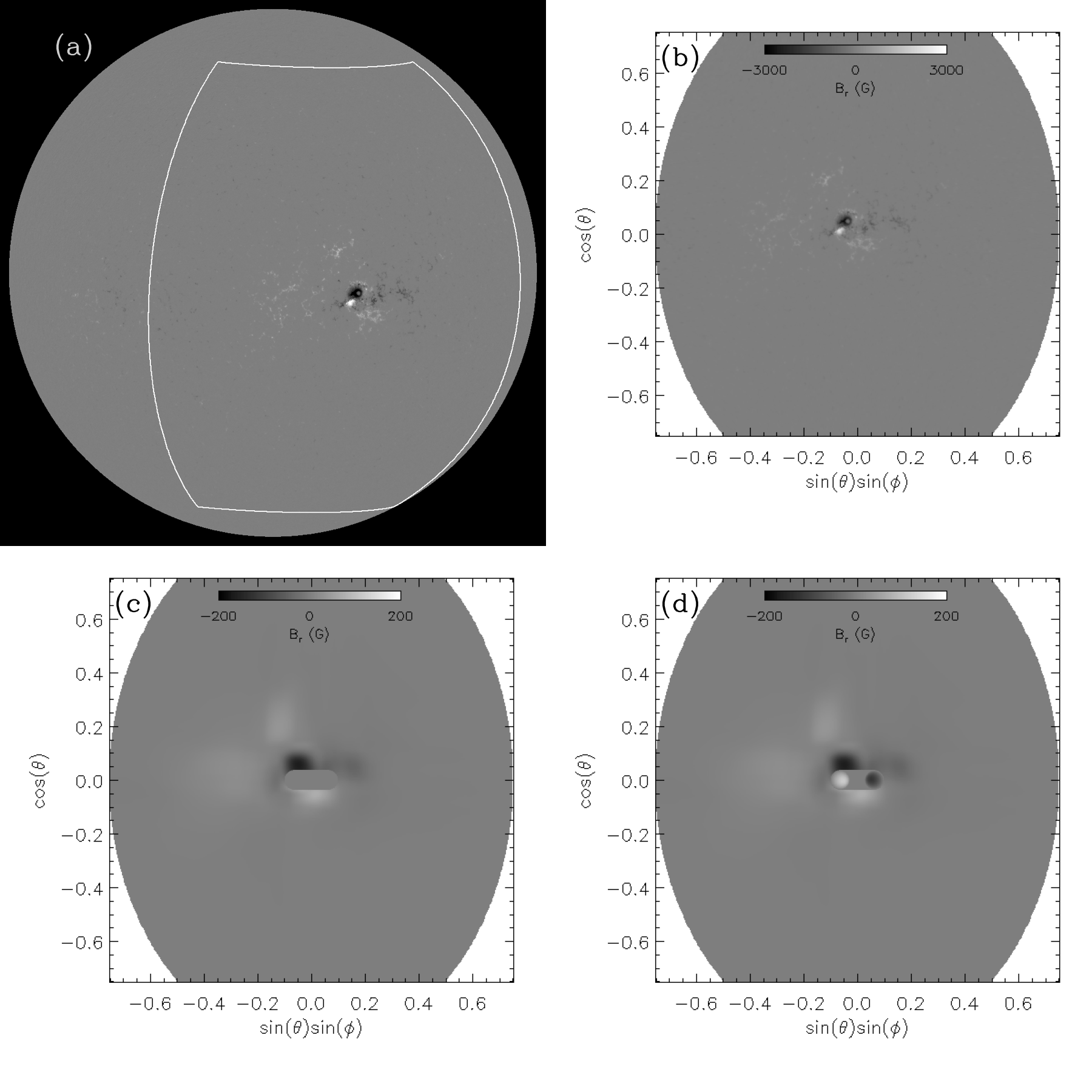
Figure 1: (a) SOHO MDI full-disk magnetogram at 20:51:01 UT on December 12, 2006. The white box encloses the area to be used as the lower boundary of the simulation domain. (b) Radial magnetic field $B_{r}$ in the region enclosed by the white box in (a) as viewed straight-on at the center of the region. (c) $B_{r}$ on the lower boundary of the simulation domain after a Gaussian smoothing has been applied and with the field in a central region zeroed out, where the emergence of a twisted magnetic torus is to be imposed. (d) $B_{r}$ on the lower boundary at the end of the simulation. A movie of the $B_{r}$ evolution on the lower boundary during the whole course of the simulation is given in the online version of the article

Similar to the simulation setup of F11, we impose at the lower boundary the emergence of the upper half of a twisted magnetic torus into a pre-existing coronal potential magnetic field. The potential field is constructed using the MDI full-disk magnetogram taken at 20:51:01 UT, December 12, 2006. However here we incorporate a much wider simulation domain compared to F11. As shown in Figure 1(a), from the MDI full-disk magnetogram, a much wider region centered on the emerging $\delta$-sunspot, corresponding to the region enclosed by the white box with a latitudinal width of $117^{\circ}$ and a longitudinal width of $98^{\circ}$, is extracted to be the lower boundary of the simulation domain. The simulation domain as described in the simulation spherical coordinate system is given by $r\in[R_{\odot},6.25R_{\odot}]$, $\theta\in[31.4^{\circ},148.6^{\circ}]$, and $\phi\in[-49.2^{\circ},49.2^{\circ}]$. The center of the white-boxed region shown in Figure 1(a) is the center of the simulation lower boundary at $\theta=90^{\circ}$ and $\phi=0^{\circ}$. We use a non-uniform grid of $576(r)\times 480(\theta)\times 504(\phi)$ that is stretched in all three dimensions to resolve the simulation domain. In $r$, the grid size is 1 Mm for $r<1.65R_{\odot}$ and then it increases geometrically, reaching about 92 Mm at the outer boundary of $6.25R_{\odot}$. Horizontally in $\theta$ and $\phi$, the grid size is about $0.00148\;rad$ (or $0.0848^{\circ}$) in the central area within $\sim 10^{\circ}$ heliographic distance from the center, and then increases geometrically to about $0.0162\;rad$ (or $0.929^{\circ}$) towards the $\theta$ boundaries, and to about $0.0131\;rad$ (or $0.748^{\circ}$) towards the $\phi$ boundaries.

For the $\theta$ and $\phi$ boundaries, we assume non-penetrating, stress-free, and electrically perfect conducting walls. For the outer $r$ boundary, we use simple outward extrapolations to allow plasma and magnetic flux to flow through. At the lower boundary, the normal magnetic field $B_{r}$ extracted from the MDI full disk magnetogram as viewed straight on the center of the region is shown in Figure 1(b). As is in F11, we apply a smoothing of $B_{r}$ using a Gaussian filter that reduces the peak field strength from about $3000$ G to $164$ G. This smoothing is done since the lower boundary density is set to be that of the base of the corona (see below), and therefore a drastic reduction of the field strength from that measured on the photosphere is made to avoid an extremely high peak Alfvén speed that would severely limit the time step of numerical integration. With the smoothed $B_{r}$, we then zero out the magnetic flux in a central area that roughly encloses the region of the observed flux emergence, including the rotating positive sunspot and the negative emerging pores to the west of it, as shown in Figure 1(c). The zeroed out area is the region on the lower boundary where we impose the emergence of a twisted magnetic torus as described below. The potential field extrapolated from the normal magnetic field shown in Figure 1(c) is used as the initial coronal magnetic field for the simulation. For the initial atmosphere we assume a static polytropic atmosphere:

$$\rho=\rho_{R_{\odot}}\left[1-\left(1-\frac{1}{\gamma}\right)\frac{GM_{\odot}}{R_{\odot}}\frac{\rho_{R_{\odot}}}{p_{R_{\odot}}}\left(1-\frac{R_{\odot}}{r}\right)\right]^{\frac{1}{\gamma-1}}$$ (1)

$$p=p_{R_{\odot}}\left[1-\left(1-\frac{1}{\gamma}\right)\frac{GM_{\odot}}{R_{\odot}}\frac{\rho_{R_{\odot}}}{p_{R_{\odot}}}\left(1-\frac{R_{\odot}}{r}\right)\right]^{\frac{\gamma}{\gamma-1}}$$ (2)

where $\rho_{R_{\odot}}=8.365\times 10^{-16}$ g ${\rm cm}^{-3}$ and $p_{R_{\odot}}=0.152$ dyne ${\rm cm}^{-2}$ are the initial density and pressure at the lower boundary, with the temperature at the lower boundary being 1.1 MK. Thus for the initial static equilibrium, the peak Alfvén speed is $21,800$ km/s in the main negative sunspot at the lower boundary, and the sound speed is $141$ km/s at the lower boundary. The Alfvén speed is greater than the sound speed in most of the simulation domain.

In the area where the flux is zeroed out on the lower boundary surface ($r=R_{\odot}$), we specify the following time dependent transverse electric field ${\bf E}_{\perp}|_{r=R_{\odot}}$ to drive the kinematic emergence of a twisted magnetic torus ${\bf B}_{\rm tube}$ at a velocity ${\bf v}_{\rm rise}$:

$${\bf E}_{\perp}|_{r=R_{\odot}}={\hat{\bf r}}\times\left[\left(-\frac{1}{c}\,{\bf v}_{\rm rise}\times{\bf B}_{\rm tube}(R_{\odot},\theta,\phi,t)\right)\times{\hat{\bf r}}\right].$$ (3)

${\bf B}_{\rm tube}$ is an axisymmetric torus specified below in its own local spherical polar coordinate system ($r^{\prime}$, $\theta^{\prime}$, $\phi^{\prime}$). The origin of the ($r^{\prime}$, $\theta^{\prime}$, $\phi^{\prime}$) coordinate system is the center of the torus, and is located at ${\bf r}={\bf r}_{c}=(r_{c},\theta_{c},\phi_{c})$ in the Sun-centered simulation spherical coordinate system $(r,\theta,\phi)$. The polar axis of the ($r^{\prime}$, $\theta^{\prime}$, $\phi^{\prime}$) coordinate system is the symmetric axis of the torus, and is parallel to the $-{\hat{\bf\theta}}$ direction at the position ${\bf r}_{c}$. In the ($r^{\prime}$, $\theta^{\prime}$, $\phi^{\prime}$) coordinate system, ${\bf B}_{\rm tube}$ is given by:

$${\bf B}_{\rm tube}=\nabla\times\left(\frac{A(r^{\prime},\theta^{\prime})}{r^{\prime}\sin\theta^{\prime}}\hat{\bf\phi^{\prime}}\right)+B_{\phi^{\prime}}(r^{\prime},\theta^{\prime})\hat{\bf\phi^{\prime}},$$ (4)

$$A(r^{\prime},\theta^{\prime})=\frac{1}{4}qa^{2}B_{t}\left(1-\frac{\varpi^{2}(r^{\prime},\theta^{\prime})}{a^{2}}\right)^{2},$$ (5)

$$B_{\phi^{\prime}}(r^{\prime},\theta^{\prime})=\frac{aB_{t}}{r^{\prime}\sin\theta^{\prime}}\left(1-\frac{\varpi^{2}(r^{\prime},\theta^{\prime})}{a^{2}}\right),$$ (6)

$$\varpi(r^{\prime},\theta^{\prime})=(r^{\prime 2}+R^{\prime 2}-2r^{\prime}R^{\prime}\sin\theta^{\prime})^{1/2},$$ (7)

where $a=0.035R_{\odot}$ is the minor radius of the torus, $R^{\prime}=0.063R_{\odot}$ is the major radius of the torus, $\varpi$ denotes the distance to the curved axis of the torus, $q/a=0.082\;{\rm rad/Mm}$ corresponds to the rate of field line twist (rad per unit length) about the curved axis of the torus, and $B_{t}a/R^{\prime}=111$ G is the field strength at the curved axis of the torus. ${\bf B}_{\rm tube}$ is truncated to zero for $\varpi>a$. The field line twist rate of the emerging torus used here is about 1.33 times that used in F11. Initially the center of the ($r^{\prime}$, $\theta^{\prime}$, $\phi^{\prime}$) coordinate system (i.e. the center of the torus) is located at ${\bf r}_{c}=(r_{c}=0.902R_{\odot},\;\theta_{c}=90^{\circ},\;\phi_{c}=0^{\circ})$. Thus the torus initially lies in the equatorial plane in the simulation coordinate system, below the lower boundary with its outer edge just touching the lower boundary. For specifying the time dependent ${\bf E}_{\perp}|_{r=R_{\odot}}$, we assume that the center of the torus ${\bf r}_{c}$ is rising at a constant velocity ${\bf v}_{\rm rise}=v_{\rm rise}{\hat{\bf r}_{c}}$ with $v_{\rm rise}=9.75$ km/s (much smaller than the Alfvén speed and the sound speed in the coronal domain). The velocity field on the lower boundary is uniformly ${\bf v}_{\rm rise}$ in the area where the emerging torus intersects the lower boundary and zero outside. Compared to F11, which used a much larger $v_{\rm rise}=98$ km/s in the early phase of emergence and then slowed down to $v_{\rm rise}=19.5$ km/s when getting closer to the onset of eruption, here we use a much slower but constant $v_{\rm rise}=9.75$ km/s to drive the emergence continuously.

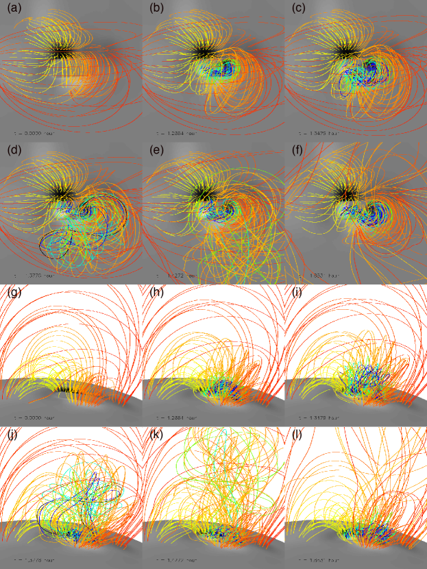
Figure 2: Snapshots of the 3-dimensional magnetic field evolution over the whole course of the simulation, with the top 2 rows showing a perspective view from the Earth’s line-of-sight, and the bottom 2 rows showing a side view. A movie of the 3D field evolution is available in the online version.

The resulting ${\bf E}_{\perp}|_{r=R_{\odot}}$ (eq. 3) produces the emergence of an east-west oriented bipolar region as shown in a movie of $B_{r}$ evolution on the lower boundary given in the online version of Figure 1, and Figure 1(d) shows a snapshot of $B_{r}$ on the lower boundary at the end of the simulation. The imposed flux emergence pattern is qualitatively representative of the observed flux emergence pattern of the region (Kubo et al., 2007; Min & Chae, 2009). It is found that the emergence of the positive rotating sunspot moving eastward is accompanied by scattered pores of negative polarity emerging and moving westward, suggesting that they are the counterparts of an east-west oriented emerging bipolar pair (see Figure 2 in Min & Chae, 2009). For our imposed flux emergence pattern (Figure 1(d) and the associated online movie) produced by the emergence of a twisted magnetic torus, the positive spot of the emerging bipolar pair corresponds to the positive rotating sunspot moving eastward along the southern edge of the large pre-existing sunspot, and the negative emerging spot represents the collection of the observed scattered negative emerging pores.

3 Results

3.1 Overview of evolution

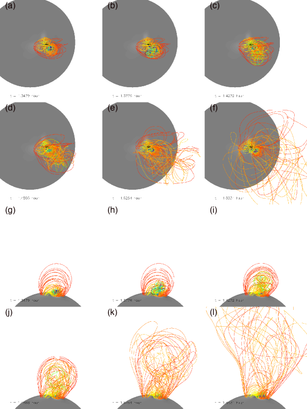
Figure 3: Snapshots showing the zoomed out views of the 3D coronal magnetic field after the onset of the eruption. Top two rows show the perspective view from the Earth’s line-of-sight, and the bottom rows show a zoomed out side view. A movie of the 3D field evolution is available in the online version.

Figure 2 shows snapshots of the evolution of the 3D coronal magnetic field over the whole course of the simulation, with the top 2 rows of images showing a perspective view from the Earth’s line-of-sight and the bottom 2 rows showing a side view. Figure 3 shows snapshots of two zoomed-out views of the 3D field evolution during the later stage of the simulation. A movie of the 3D field evolution combining the 4 views shown in the above two figures is available in the online version. We trace the field lines shown in Figures 2 and 3 in the following way. We use a set of fixed foot points in the ambient field region outside of the emerging flux region to trace the red, orange, and yellow field lines. For tracing the field lines (green, blue, and black field lines) from the emerging flux region on the lower boundary, we track a set of foot points that connect to the same field lines of the subsurface emerging torus and the field lines are colored based on the flux surfaces of the subsurface torus. Figures 2(a)(g) show the initial potential magnetic field, which is constructed using the lower boundary $B_{r}$ shown in Figure 1(c). With time a twisted coronal flux rope (as represented by the green, blue and black field lines in Figures 2(b)(h)) is built up quasi-statically, as a result of the imposed flux emergence at the lower boundary described in Section 2.

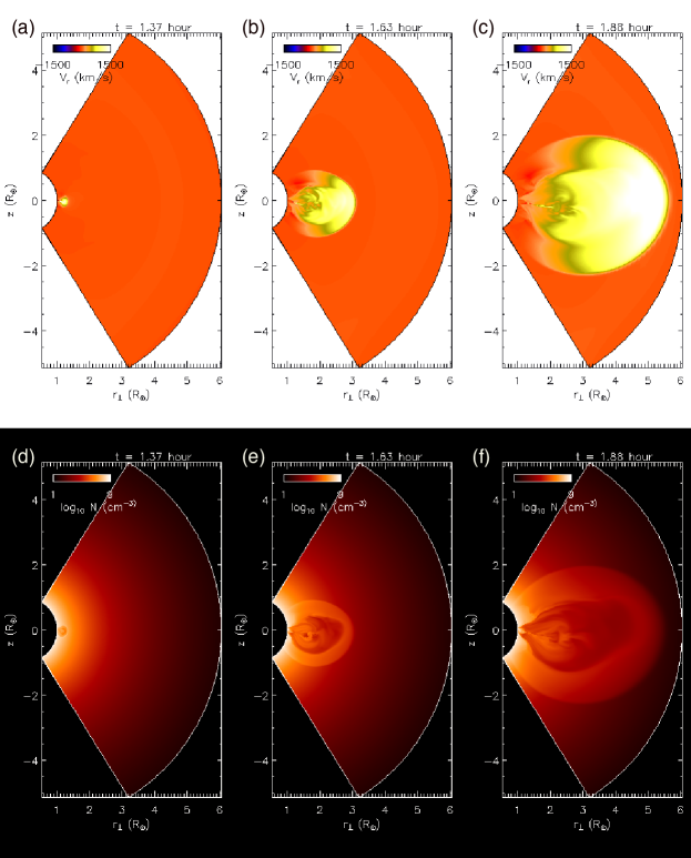
Figure 6: (Top panels) Snapshots of the evolution of the radial velocity $V_{r}$ in the central meridional cross-section of the erupting flux rope. (Bottom panels) Same as the top panels but showing the density. A movie of the evolution of both $V_{r}$ and the density in the central meridional cross section is available in the online version.

Figure 4 shows the evolution of the free magnetic energy (top panel), which is the total magnetic energy $E_{m}$ minus the energy $E_{p}$ of the corresponding potential magnetic field extrapolated using the current normal magnetic field distribution at the lower boundary, and the evolution of the kinetic energy $E_{k}$ (bottom panel). Figure 5 shows the rise velocity at the apex of the axial field line of the coronal flux rope (diamond points), which connects to the axial field line of the subsurface emering torus, and the rise velocity at the front of the erupting coronal flux rope cavity (cross points) in the later time period. From $t=0$ to roughly $t=1.3$ hour, the coronal magnetic field evolves quasi-statically, with the free magnetic energy being built up (top panel of Figure 4), and with the coronal flux rope emerges and rises quasi-statically with very small rise velocity (Figure 5). The coronal flux rope begins to erupt at about $t=1.3$ hour, where the free magnetic energy undergoes a significant decrease, the kinetic energy undergoes a rapid increase (see Figure 4), and the flux rope axis shows a rapid acceleration (Figure 5). Figures 2(c)(d)(e)(i)(j)(k) (also the associated animation in the online version of the paper) show that the flux rope field rooted in the emerging region (green, blue, and black field lines) erupts upward, pushing the ambient field (red, orange, yellow field lines) outward, and shows a counter-clockwise rotation as it erupts. The apex of the axial field line accelerate to about $1300$ km/s (diamond points in Figure 5) before it reconnects. Subsequently we track the rise velocity at the front of the erupting flux rope cavity (cross points in Figure 5) and find that its rise speed increases to over $1500$ km/s at the end of the simulation when it reaches about 4.5 $R_{\odot}$. Figure 6 shows snapshots of the evolution of the radial velocity $V_{r}$ in the central meridional plane across the erupting flux rope (top panels), and the corresponding evolution of the density in the same meridional plane (bottom panels). A movie showing the evolution of $V_{r}$ and density in the meridional plane is also available with the online version of the figure. We see the development of a wide ejecta, which consists of a central low density cavity region (containing the twisted erupting flux rope) surrounded by a denser sheath (Figures 6(d)(e)(f)). Compare Figure 6(d) here with Figure 7 in F11. They are both showing roughly the same stage of the eruption when the front of the flux rope cavity reaches about 1.3 $R_{\odot}$. In F11, the erupting flux rope is already hitting the south boundary wall because of the narrow simulation domain used there. As a result the subsequent acceleration of the flux rope becomes severely impeded and the speed measured at the front of the flux rope cavity becomes saturated at about 830 km/s as shown in Figure 6 of F11. Here with the significantly widened simulation domain (see Figures 6 (d)(e)(f)), we are able to follow the subsequent acceleration and evolution of the flux rope. The front of the sheath and the front of the cavity are found to attain a speed of about $1500$ km/s at the end of the simulation (see Figures 6(c)(f)). The velocity shown by the cross points in Figure 5 is measured at the front edge of the cavity on the $z=0$ line in the meridional plane shown in Figure 6.

As the twisted flux rope erupts, it continually reconnects with the ambient coronal magnetic field, and towards the end of the simulation, the outward erupting fields have become entirely rooted in the ambient field region outside of the emerging flux region on the lower boundary. This can be seen in Figures 3(e)(f)(k)(l), where the red, orange, and yellow colors of the erupting field lines indicate that they are rooted in the ambient field region (see more description later in Section 3.3). Furthermore, due to the continued flux emergence, the free magnetic energy is built up again after the rapid release of the first eruption (see top panel of Figure 4) and a new closed twisted flux rope has reformed connecting the emerging bipolar region, poised for a second eruption (see the blue and green field lines in Figures 2(f)(l)). From the movie associated with the online version of Figure 2, it can be seen that the reformed flux rope has begun to accelerate for the second eruption at the end of the simulation at about $t=1.88$ hour.

3.2 Onset of the eruption

At the onset of the eruption at about $t=1.3$ hour, the twist of the field lines about the axis of the emerged flux rope has reached about $1.2$ winds between their anchored ends. Therefore the flux rope is close to the threshold of twist ($2.49\pi$ or about $1.25$ winds) for the onset of the helical kink instability (e.g. Hood & Priest, 1981). The $1.2$ winds (or $432^{\circ}$ rotation) of field line twist in the emerged flux rope is within the observed range of the total twist transported into the corona as measured by the rotation of the emerging positive sunspot: at least $240^{\circ}$ obtained by Zhang et al. (2007), and $540^{\circ}$ obtained by Min & Chae (2009). We also show in the bottom panel of Figure 7, $d\ln(B_{p})/d\ln(H)$, the decay rate with height $H$ of the corresponding potential magnetic field $B_{p}$ along the central vertical slice in the central meridional plane across the flux rope, and in the top panel of Figure 7, the profile of $\alpha\equiv(\nabla\times{\bf B})\cdot{\bf B}/B^{2}$ along the same vertical slice. The value of $\alpha$ is a measure of the twist rate of the magnetic field, and the height range where $\alpha$ is significantly negative indicates the height range of the flux rope cross-section. We see from Figure 7 that the top of the flux rope cross-section has reached about $H=0.15R_{\odot}$ as marked by the vertical dotted lines and that the top portion of the flux rope has reached the region where the decay rate of the potential magnetic field $-d\ln(B_{p})/d\ln(H)$ has exceeded the magnitude of 1.5, which is the threshold for the flux rope to develop the torus instability (e.g Kliem & Török, 2006; Isenberg & Forbes, 2007). Thus both the helical kink instability and the torus instability are likely playing a role in triggering the eruption of the coronal flux rope. We found that with a wider simulation domain and the inclusion of a wider range of the observed ambient normal flux distribution on the lower boundary, the magnitude of the decay rate of the potential field is greater compared to that obtained for F11, in the lower height range from 0 to $0.6R_{\odot}$. This might have contributed to a higher terminal speed of the erupting flux rope in the present case (e.g. Török & Kliem, 2007). However, the dominant reason for the lower saturation speed of the front of the flux rope found in F11 is due to the side wall boundary which begins to impede the acceleration of the flux rope soon after the onset of the eruption (see Figure 7 of F11).

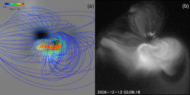
Figure 8: 3D field lines (colored based on the temperature) of the coronal magnetic field (with the central heated field lines densely traced) at a time ($t=1.26$ hour) just before the onset of the eruption viewed from the Earth’s line of sight, compared with the Hinode XRT image of the region just prior to the onset of the flare (b). Panel (b) is reproduced from Figure 8(e) in F11

Figure 8 shows 3D field lines (colored based on the temperature) of the coronal magnetic field at a time ($t=1.26$ hour) just before the onset of the eruption (panel (a)), compared with the Hinode X-Ray Telescope (XRT) image of the region just prior to the onset of the flare (panel (b)). Similar to F11, we find that the central core field of the flux rope is strongly heated because of the formation of a sigmoid shaped current layer. In Figure 8(a) we have densely traced these highly heated field lines, whose temperature has reached about 10 MK. The heated sigmoid shaped core field may give rise to the bright sigmoid loops in the pre-eruption region observed in Hinode XRT images (Figure 8(b), also Su et al., 2007, see their Figure 1).

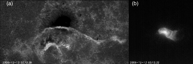
Figure 9: (a) Hinode SOT image in Ca II line showing the chromosphere flare ribbon brightening, and (b) Hinode XRT image showing the soft X-ray post flare loop brightening. This figure is reproduced from Figures 9(c)(d) in F11

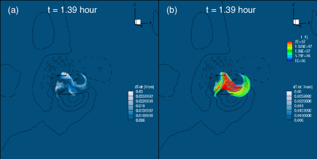
Figure 10: (a) Image showing the vertical gradient of temperature increase on the lower boundary overlaid with the line contours showing the normal magnetic field with solid contours (dashed contours) representing positive (negative) magnetic polarity. (b) Same as (a) but also showing field lines with foot points rooted in the bright ribbons in (a). The field lines are colored based on temperature.

After the flare onset, the soft X-ray emission becomes completely dominated by the brightening of a sigmoid-shaped row of post-flare loops as shown in a Hinode XRT image in Figure 9(b), and the corresponding Hinode Solar Optical Telescope (SOT) observation (Figure 9(a)) shows the two-ribbon brightening in the lower atmosphere. The two bright ribbons correspond to the foot points of the heated post flare loops, where energetic electrons and downward heat conduction along the post reconnection loops cause heating and brightening in the lower atmosphere. In Figure 10(a) we show an image of the gradient of temperature increase with height at the lower boundary, which is a measure of the downward heat conduction along the loops rooted there. This is shown at time $t=1.39$ hour, just after the peak acceleration of the eruption. It marks the location of the foot points of strongly heated loops as a result rapid reconnection in the simulation. We see two curved bright ribbons, which show some similarities in their paths and locations in relation to the normal magnetic flux distribution (contours in Figure 10(a)) as the observed flare ribbons. For the upper ribbon, its east part extends into the dominant negative pre-existing sunspot and its west part curves about the emerging negative polarity region which corresponds to the emerged, fragmented negative pores to the west of the main negative sunspot in the observation. The lower ribbon has an overall arc shape and cuts across the main positive emerging sunspot. We also plotted field lines with foot points rooted in the bright ribbons and color the field lines based on temperature as shown in Figure 10(b). We see that these field lines form a sigmoid-shaped row of heated loops showing an overall morphology similar to that of the X-ray post flare loop brightening seen in the XRT observation (Figure 9).

3.3 Evolution of the erupting flux rope

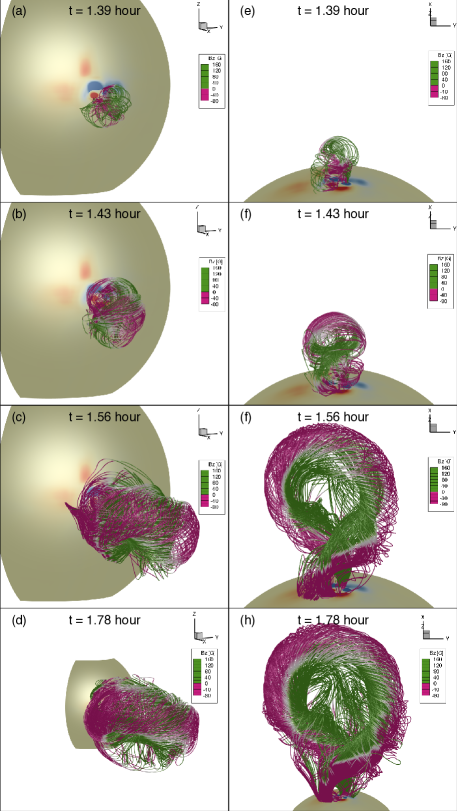
Figure 11: Snapshots of the 3D field lines of the erupting flux rope, with the left column images showing a view from the Earth’s line-of-sight and the right column images showing a side view. The field lines are colored based on the sign of the north-south component of the magnetic field $B_{z}$. The color on the sphere shows the normal magnetic field strength on the lower boundary with red (blue) corresponding to positive (negative) field. The bottom images are more zoomed out views as indicated by the smaller size of the Sun

By densely tracing field lines inside the erupting cavity (whose cross-section can be seen in the meridional cross-section plots of density in Figure 6), we examine the structure and evolution of the erupting flux rope. Figure 11 shows snapshots of the 3D field lines in the erupting flux rope, with the field lines colored based on the sign of the north-south component of the magnetic field $B_{z}$, with green (purple) indicating positive (negative) $B_{z}$. The left column images show the view from the Earth’s line-of-sight, and the right column images shows a side view. The bottom images show more zoomed out views at a later time (as indicated by the smaller size of the Sun compared to the other panels). At the onset of the eruption, the $B_{z}$ for the top of the flux rope and also the overlying potential field above the flux rope is positive or northward (green). Immediately after the onset of the eruption, the erupting flux rope rotates counter-clockwise when viewed from above, as can be seen in Figure 11. This direction of rotation is consistent with the left-handed twist of the pre-eruption flux rope (e.g. Fan & Gibson, 2004; Fan, 2005). By the time the top of the flux rope has reached about $r=2.4R_{\odot}$ (Figures 11(c)(f)), the flux rope has rotated by about $180^{\circ}$ and the $B_{z}$ of the entire outer circumference of the flux rope has become negative or southward directed. Later the erupting flux rope seems to continually expand outward without further significant change of its orientation, and both the front and flank of the expanding flux rope maintains southward directed $B_{z}$ as can be seen in the zoomed out views of the later evolution shown in Figures 11(d)(h). This orientation of the expanding flux rope, if maintained in the propagation in the solar wind to the Earth, would explain the southward directed magnetic field for the front of the magnetic cloud (MC) impacting the Earth (e.g. Liu et al., 2008). This southward directed $B_{z}$ for the front of the MC appears opposite to the northward $B_{z}$ for the top of the pre-existing flux rope and the overlying potential field in the CME source region on the Sun. The large ($\sim 180^{\circ}$) counter-clockwise rotation of the flux rope achieved during the initial phase of the eruption is consistent with the large left-handed twist (more than 1 wind of field-line rotation about the axis) stored in the pre-eruption flux rope.

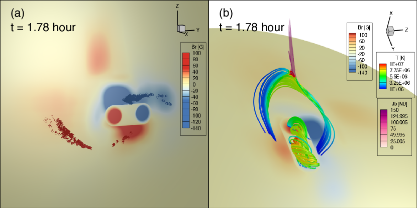
Figure 12: (a) The foot points of the field lines of the erupting flux rope in Figures 11(d)(h) plotted on the lower boundary against the normal magnetic field $B_{r}$. The foot points are colored based on the polarity region in which they are located, red for positive normal field and blue for negative. (b) Selected field lines (colored based on the temperature) showing the field lines of the reformed twisted flux rope connecting the emerging bipolar region under a set of cusped field lines just reconnected in the overlying vertical current sheet (represented by the purple iso-surface of $J_{b}\equiv|\nabla\times{\bf B}|/B=1/(5dr)$, where $dr$ is the radial grid size)

We find that due to continued magnetic reconnection, the erupting flux rope evolves to become completely rooted in the ambient pre-existing normal flux distribution, outside of the emerging bipolar region, as shown in Figure 12(a) where the foot points of the field lines of the erupting flux rope in Figures 11(d)(h) are plotted on the lower boundary against the normal magnetic field distribution. Thus we expect the coronal dimmings, produced by plasma depletion in flux tubes of the stretched out fields of the CME, to form outside of the emerging bipolar region, away from the main flare site (e.g. Gibson & Fan, 2008; Attrill et al., 2010; Imada et al., 2011). Figure 12(b) shows that, a new twisted flux rope connecting the emerging bipolar region with sigmoid shaped field lines reforms due to continued flux emergence, under the cusped loops which have just reconnected in the overlying vertical current sheet (the purple iso-surface). The reformation of the flux rope and the associated buildup of the free magnetic energy after the magnetic energy release of the first eruption (see upper panel of Figure 4) are setting up for a second eruption. This may qualitatively explain the buildup for a second X-class flare and CME in the same region the following day on December 14.

4 Discussions and Conclusions

Improving upon the previous work of F11, we have carried out an MHD simulation to qualitatively model the magnetic field evolution of the eruptive flare and CME on 13 December 2006 in the emerging $\delta$-sunspot region AR 10930. The main improvement compared to F11 is the significantly widened simulation domain and the inclusion of a much more extended region of the observed photospheric normal flux distribution in the construction of the pre-existing coronal potential field. In this way the simulation can accommodate the wide CME (see Figure 6) and better determine the structure and dynamic evolution of the erupting flux rope without it being severely constrained by the boundaries immediately after the onset of the eruption as was the case in F11.

Guided by the observed photospheric magnetic flux emergence pattern in AR 10930 (e.g. Kubo et al., 2007; Min & Chae, 2009; Ravindra et al., 2011), we impose the emergence of an east-west oriented, left-hand twisted flux rope at the lower boundary. The resulting flux emergence pattern is such that the positive emerging polarity corresponds to the observed positive (counter-clockwise) rotating sunspot emerging against the south end of the pre-existing dominant negative sunspot, and the negative emerging polarity corresponds to the collection of the fragmented negative pores observed to emerge to the west of the $\delta$-spot (Min & Chae, 2009). As a result of the flux emergence, a twisted coronal flux rope confined by the pre-existing potential coronal field constructed based on the observed ambient photospheric magnetic field is built up quasi-statically. The resulting pre-eruption coronal magnetic field shows heated, inverse-S shaped core fields with morphology similar to the bright sigmoid-shaped loops in the pre-eruption region observed in soft X-ray images by Hinode XRT.

The flux rope is found to erupt after its field line twist about the axis has reached about 1.2 winds, close to the threshold for the onset of the helical kink instability, and its upper half of the cross-section has entered the height where the decline rate of the corresponding potential field has exceeded the thresh hold for the onset of the torus instability. The twist of the flux rope at the onset of eruption is within the measured range of twist transported into the corona based on the observation of the rotating positive sunspot. Using a measure of the downward heat conduction flux at the lower boundary as the proxy for the location of the flare ribbons, we found that the path and locations of the ribbons in relation to the normal magnetic flux distribution show qualitative similarities as the observed flare ribbons in the lower solar atmosphere observed by the Hinode SOT. Also the field lines rooted in the bright ribbons form a sigmoid-shaped row of heated loops that show similar morphology to the observed X-ray post flare loop brightening.

The initial potential field overlying the coronal flux rope and also the top of the left-hand twisted coronal flux rope of the source region are both having northward directed (positive) $B_{z}$ field. However, immediately after the onset of the eruption, the erupting flux rope in the cavity is found to undergo a counter-clockwise rotation (as viewed from above) by about $180^{\circ}$ such that its entire front and flanks are showing southward directed (negative) $B_{z}$ field (see Figure 11). This large rotation of the erupting flux rope is accomplished in the early phase of the eruption and later the flux rope shows mainly outward expansion without further significant change of orientation (see Figures 11(c)(d) and Figures 11(f)(h)). The orientation of such an expanding flux rope in the CME ejecta, if maintained during its propagation in the solar wind, may explain the southward directed magnetic field in the front part of the magnetic cloud impacting the Earth (e.g. Liu et al., 2008). The front of the erupting flux rope is found to accelerate to a terminal speed of about $1500$ km/s, which is still smaller than the observationally measured range of $1780$ km/s to $3060$ km/s for the CME speed determined from SOHO Large Angle and Spectrometric Coronagraph (LASCO) observations (e.g. Ravindra & Howard, 2010). Our simulation also shows that the source region coronal magnetic field driven by the continued flux emergence is capable of reformation of the flux rope and a second eruption and hence explaining the observed occurrence of another eruptive flare on December 14, 2006 from the same region.

Our MHD simulation driven by the emergence of an east-west oriented magnetic flux rope is aimed to model qualitatively the structure and topology of the magnetic field for both the source region and the CME ejecta of the eruptive flare on December 13, 2006. There are many severe limitations of the model. The smoothing of the observed photospheric field to reduce the peak field strength at the lower boundary to under $200$ G, due to numerical constraints, greatly under estimates the free magnetic energy buildup (about $4\times 10^{31}$ ergs) and release ($\sim 10^{31}$ ergs) for the resulting CME (Figure 4), compared to the observational estimates (on the order of $10^{32}$ ergs) for the CME energy (e.g. Schrijver et al., 2008; Ravindra & Howard, 2010). This would lead to an under estimate of the CME speed. Also, our simulation assumes an initial potential field without an ambient solar wind. All of these simplifications can affect the resulting CME speed and energetics. Further improvement of the model with more realistic lower boundary conditions and the inclusion of an ambient solar wind with more realistic treatment of the thermodynamics are needed to achieve a quantitative description of the event. Progress is being made in using high-cadence vector magnetic field and Doppler velocity observations by the Helioseismic and Magnetic Imager (HMI) of the Solar Dynamics Observatory (SDO) to infer the electric field evolution at the photosphre of flare/CME productive active regions (e.g. Kazachenko et al., 2014, 2015). Such observationally inferred electric fields may be used for constructing more realistic lower boundary driving conditions of flux emergence for the MHD simulations of the CME events.

Figure 4: Top panel: the evolution of the free magnetic energy, which is the total magnetic energy $E_{m}$ minus the energy $E_{p}$ of the corresponding potential magnetic field extrapolated using the current normal magnetic field distribution at the lower boundary. Bottom panel: the evolution of the kinetic energy.

Figure 5: The rise velocity of the axis of the coronal flux rope that forms and then erupts (diamond points) and the rise velocity at the front of the cavity of the erupting flux rope (cross points).

Figure 7: Top panel shows the profile of $\alpha\equiv(\nabla\times{\bf B})\cdot{\bf B}/B^{2}$ along the central vertical slice in the central meridional plane across the flux rope. Bottom panel shows $d\ln(B_{p})/d\ln(H)$, the decay rate with height $H$ of the corresponding potential magnetic field $B_{p}$ along the same vertical slice. $R_{s}$ denotes the solar radius. The value of $\alpha$ is a measure of the twist rate of the magnetic field, and the height range where $\alpha$ is significantly negative indicates the height range of the flux rope cross-section, and thus the vertical dotted lines marks the top of the flux rope cross section.

.

References

- Attrill et al. (2010) Attrill, G. D. R., Harra, L. K., van Driel-Gesztelyi, L., & Wills-Davey, M. J. 2010, Sol. Phys., 264, 119
- Downs et al. (2015) Downs, C., Török, T., Titov, V., et al. 2015, in AAS/AGU Triennial Earth-Sun Summit, Vol. 1, AAS/AGU Triennial Earth-Sun Summit, 304.01
- Fan (2005) Fan, Y. 2005, ApJ, 630, 543
- Fan (2011) —. 2011, ApJ, 740, 68
- Fan (2012) —. 2012, ApJ, 758, 60
- Fan & Gibson (2004) Fan, Y., & Gibson, S. E. 2004, ApJ, 609, 1123
- Gibson & Fan (2008) Gibson, S. E., & Fan, Y. 2008, Journal of Geophysical Research (Space Physics), 113, A09103
- Gosain et al. (2009) Gosain, S., Venkatakrishnan, P., & Tiwari, S. K. 2009, ApJ, 706, L240
- Hood & Priest (1981) Hood, A. W., & Priest, E. R. 1981, Geophysical and Astrophysical Fluid Dynamics, 17, 297
- Imada et al. (2011) Imada, S., Hara, H., Watanabe, T., et al. 2011, ApJ, 743, 57
- Isenberg & Forbes (2007) Isenberg, P. A., & Forbes, T. G. 2007, ApJ, 670, 1453
- Kataoka et al. (2009) Kataoka, R., Ebisuzaki, T., Kusano, K., et al. 2009, Journal of Geophysical Research (Space Physics), 114, A10102
- Kazachenko et al. (2014) Kazachenko, M. D., Fisher, G. H., & Welsch, B. T. 2014, ApJ, 795, 17
- Kazachenko et al. (2015) Kazachenko, M. D., Fisher, G. H., Welsch, B. T., Liu, Y., & Sun, X. 2015, ApJ, 811, 16
- Kliem & Török (2006) Kliem, B., & Török, T. 2006, Physical Review Letters, 96, 255002
- Kubo et al. (2007) Kubo, M., Yokoyama, T., Katsukawa, Y., et al. 2007, PASJ, 59, S779
- Liu et al. (2008) Liu, Y., Luhmann, J. G., Müller-Mellin, R., et al. 2008, ApJ, 689, 563
- Mikic et al. (2008) Mikic, Z., Linker, J. A., Lionello, R., et al. 2008, AGU Spring Meeting Abstracts
- Min & Chae (2009) Min, S., & Chae, J. 2009, Sol. Phys., 258, 203
- Ravindra & Howard (2010) Ravindra, B., & Howard, T. A. 2010, Bulletin of the Astronomical Society of India, 38, 147
- Ravindra et al. (2011) Ravindra, B., Venkatakrishnan, P., Tiwari, S. K., & Bhattacharyya, R. 2011, ApJ, 740, 19
- Schrijver et al. (2008) Schrijver, C. J., De Rosa, M. L., Metcalf, T., et al. 2008, ApJ, 675, 1637
- Su et al. (2007) Su, Y., Golub, L., van Ballegooijen, A., et al. 2007, PASJ, 59, S785
- Titov et al. (2008) Titov, V. S., Mikic, Z., Linker, J. A., & Lionello, R. 2008, ApJ, 675, 1614
- Török & Kliem (2007) Török, T., & Kliem, B. 2007, Astronomische Nachrichten, 328, 743
- Zhang et al. (2007) Zhang, J., Li, L., & Song, Q. 2007, ApJ, 662, L35
.