Lorentz atom revisited by solving Abraham–Lorentz equation of motion

Abstract

By solving the non–relativistic Abraham-Lorentz (AL) equation, I demonstrate that AL equation of motion is not suited for treating the Lorentz atom, because a steady–state solution does not exist. The AL equation serves as a tool, however, for deducing appropriate parameters $\Omega,\Gamma$ to be used with the equation of forced oscillations in modelling the Lorentz atom. The electric polarizability, which many authors “derived” from AL equation in recent years, is found to violate Kramers–Kronig relations rendering obsolete the extracted photon–absorption rate, for example. Fortunately, errors turn out to be small quantitatively, as long as light frequency $\omega$ is neither too close to nor too far from resonance frequency $\Omega$. Polarizability and absorption cross section are derived for the Lorentz atom by purely classical reasoning and shown to agree with quantum–mechanical calculations of the same quantities. In particular, oscillator parameters $\Omega,\,\Gamma$ deduced by treating the atom as a quantum oscillator are found equivalent to those derived from classical AL equation. The instructive comparison provides a deep insight into understanding the great success of Lorentz’s model which was suggested long before the advent of quantum theory.

I Introduction

In recent years, the classical Lorentz–oscillator model serving as an intuitive description of an atom under the influence of the $ac$–electric field associated with a standing wave of visible light has celebrated a revival in quantum–optics literature gwo:00 , gaf:10 . While the classical equation of forced oscillations, with a friction force proportional to the $1^{\rm st}$ time–derivative of elongation, has many applications (e. g., the $ac$–current circuit with impedance and capacity bes.b:61 or simplified models of density fluctuations in liquids mar:68 ) besides the Lorentz atom, the latter has played a special role. When deriving the so–called ‘radiative reaction force’ from classical electrodynamics to account for energy loss of an accelerated charge by radiation, Abraham and Lorentz (AL) arrived at a modified equation of motion with a friction force proportional to the $3^{\rm rd}$ time–derivative of the oscillator elongation. The radiative reaction force has been discussed extensively for more than 100 years, both for relativistic and non–relativistic velocities of the charged particle, because its implications have raised fundamental problems such as “pre–acceleration” or “run–aways in the absence of external forces” which are still open for discussion (see, e. g., (jac:62, , Ch. 17), mur:77 , jic:87 , (gri:99, , Ch. 11)). In case of the Lorentz atom, the oscillating electron may be described non–relativistically. So the non–relativistic AL equation, only, will be studied here.

In Sec. II, a concise review is presented of the unique solution of the forced–oscillations equation, inclusive of its steady–state limit, by introducing classical elongation response and relaxation functions.

In Sec. III, the unique solution of the AL equation for given initial values $(x_{0},\,v_{0},\,b_{0})$ is determined. The unique solution is shown to be a “run–away” implying non–existence of a steady–state solution and spotting the AL equation of motion as an inappropriate tool for describing the Lorentz atom. The forced–oscillation equation is suggested, instead, to do the job together with oscillator parameters $(\Omega,\,\Gamma)$ derived from AL equation. In this context, a widely spread error is pointed out regarding the “complex polarizability” of the Lorentz atom (see, e. g., (jac:62, , Sec. 17.9), (gwo:00, , Sec. II.A), (gaf:10, , Sec. 2A)).

In Sec. IV, for a quantum–mechanical system perturbed by an oscillatory external field, a representation–free perturbation expansion in the field strength is presented for an expectation value. With its help, the ‘absorbed power’ (dipole moment to $1^{\rm st}$ order) and the ‘$ac$–Stark shift’ (energy to $2^{\rm nd}$ order) are derived in terms of the dipole–dipole response function, or rather the complex polarizability. The quantum–mechanical response function is evaluated for a charged quantum oscillator and compared to the classical dipole–response function of the Lorentz atom derived in Sec. III. Perfect agreement between classical and quantum–mechanical calculation is found, which renders an explanation for the great success of the classical Lorentz atom.

In Sec. V, the reader finds a Summary and Conclusions. In Sec. VI, Appendix, the unique solution of the AL equation of motion for given initial values ($x_{0},\,v_{0},\,b_{0}$) is presented in terms of classical response and relaxation functions. In addition, the Appendix contains a short compendium on integral transforms used in this work.

II Classical oscillator

II.1 Response and relaxation functions

The ordinary second–order differential equation

$$\ddot{x}(t)+\Gamma\dot{x}(t)+\Omega^{2}x(t)=f(t)/m$$ (1)

with positive constants ($m,\,\Omega,\,\Gamma$) and external force $f(t)$ has for given initial values,

$$x_{0}=x(t_{0})\;,~{}~{}~{}~{}~{}~{}~{}~{}~{}~{}~{}~{}~{}~{}~{}~{}~{}v_{0}=\dot{x}(t_{0})\;,$$ (2)

a unique solution. Finding this solution belongs to the first exercises in every math course on ordinary differential equations. For physical applications, it is useful to cast the unique solution into the intuitive form ($t\geq t_{0}$),

$$x(t;t_{0}) = \phi(t-t_{0})x_{0}+{\rm i}\chi(t-t_{0})mv_{0}$$

$$\hskip 40.00006pt+\int_{t_{0}}^{t}{\!\rm d}t^{\prime}~{}{\rm i}\chi(t-t^{\prime})f(t^{\prime})\;,$$

with abbreviations

$$\chi(t)=\frac{{\rm e}^{\zeta_{1}t}-e^{\zeta_{2}t}}{{\rm i}m(\zeta_{1}-\zeta_{2})}\;,~{}~{}~{}~{}~{}~{}\phi(t)=\frac{\zeta_{1}{\rm e}^{\zeta_{2}t}-\zeta_{2}{\rm e}^{\zeta_{1}t}}{\zeta_{1}-\zeta_{2}}~{}~{}~{}~{}~{}(t\geq 0)$$ (4)

denoting, resp., classical elongation–response and (normalized) –relaxation function defined, at this stage, for non–negative arguments, only. Here $\zeta_{1}$ and $\zeta_{2}$ denote roots of the characteristic polynomial associated with Eq. (1), $\zeta_{1,\,2}=-\Gamma/2\pm\sqrt{(\Gamma/2)^{2}-\Omega^{2}}$, which obey

$$\Re[\zeta_{1,\,2}]<0\;,~{}~{}~{}~{}~{}~{}~{}\zeta_{1}\zeta_{2}=\Omega^{2}\;,~{}~{}~{}\zeta_{1}+\zeta_{2}=-\Gamma\;.$$ (5)

Due to negative real parts of both roots $\zeta_{1}$ and $\zeta_{2}$, the functions $\phi(t)$ and $\chi(t)$ will decay to zero if time arguments grow large.

It is convenient to extend the definitions of response and relaxation functions to negative time arguments. In accordance with quantum–mechanical linear–response theory (see Sec. IV below), I postulate

$$\chi(-t)=-\chi(t)=\chi(t)^{*}\;,~{}~{}~{}~{}~{}\phi(-t)=\phi(t)=\phi(t)^{*}\;.$$ (6)

After introducing phase angle $\vartheta$ and frequency $\tilde{\Omega}$ by

$$\vartheta=\arctan\left[\frac{\Gamma}{2\tilde{\Omega}}\right],~{}~{}\tilde{\Omega}=\left\{\begin{array}[]{cc}\sqrt{\Omega^{2}-(\Gamma/2)^{2}}&,~{}\Omega>\Gamma/2\\ {\rm i}\sqrt{(\Gamma/2)^{2}-\Omega^{2}}&,~{}\Omega\leq\Gamma/2\end{array}\right.\;,$$ (7)

which will be real valued, if $\Gamma<2\Omega$ (low–damping regime), the response and relaxation functions may be expressed in the more descriptive way,

$$\chi(t)={\rm e}^{-\frac{\Gamma}{2}|t|}\,\frac{\sin(\tilde{\Omega}t)}{{\rm i}m\tilde{\Omega}}\;,~{}~{}\phi(t)={\rm e}^{-\frac{\Gamma}{2}|t|}\,\frac{\cos(\tilde{\Omega}|t|-\vartheta)}{\cos\vartheta}\;.$$ (8)

Here occurrence of $|t|$ reflects the symmetry introduced in Eq. (6).

II.2 Steady–state elongation

The initial time $t_{0}$ in Eqs. (2),(II.1) is properly interpreted as the instant, when the external force $f(t)$ is switched on. After switch–on, the elongation $x(t,t_{0})$ will at first depend on $t_{0}$ and initial values ($x_{0},\,v_{0}$) until ‘transients’ have died off due to relaxation processes, and the system described by Eq. (1) acquires a steady state. The corresponding steady–state elongation $\xi(t)$ is found by switching on the force $f(t)$ adiabatically and choosing $t_{0}=-\infty$ in Eq. (II.1),

$$\xi(t)=\lim_{t_{0}\to-\infty}x(t,t_{0})=\int_{0}^{\infty}{\!\rm d}t^{\prime}~{}{\rm e}^{-ot^{\prime}}{\rm i}\chi(t^{\prime})f(t-t^{\prime})\;.$$ (9)

Adiabatical switch–on is described by replacing under the integral in Eq. (II.1): $f(t^{\prime})\to f(t^{\prime}){\rm e}^{-o(t-t^{\prime})}$ ($o>0$). Subsequent substitution $t-t^{\prime}\to t^{\prime}$ results in Eq. (9). It is understood from here on that $o\to 0$ is taken after time integrations have been performed —without repeatedly employing the explicit notation $\lim_{o\to 0}$. This convention regarding treatment of the small positive frequency $o$ will be used throughout.

It is to be noted that the steady–state elongation Eq. (9) is independent of initial values $(x_{0},\,v_{0})$, because the general solution of the homogeneous equation (Eq. (1) for $f(t)\!\equiv\!0$), $x^{\rm h}(t,t_{0})=\phi(t-t_{0})x_{0}+{\rm i}\chi(t-t_{0})mv_{0}$ which does depend on initial conditions, will vanish in the steady–state limit. This independence of initial values is a physical requirement on a steady–state solution, because initial values $x_{0}$ and $v_{0}$ are not (and cannot usually be) measured.

II.3 Dynamical susceptibility

If the force entering the integrand in Eq. (9) is represented by its Fourier integral, the steady–state solution will also appear in Fourier–expanded form,

$$\xi(t)=\frac{1}{2\pi}\int_{-\infty}^{\infty}{\!\rm d}\omega~{}\xi_{\omega}\exp(-{\rm i}t\omega)\;,~{}~{}~{}~{}~{}~{}\xi_{\omega}=\tilde{\chi}(\omega+{\rm i}o)f_{\omega}\;,$$ (10)

with the dynamical susceptibility $\tilde{\chi}(\omega+{\rm i}o)=\xi_{\omega}/f_{\omega}$ determining the ratio between Fourier–transformed elongation and force. Here $\tilde{\chi}(z)$, the Fourier–Laplace transform (FLT, see Sec.VI.2 for details) of the response function $\chi(t)$, has been introduced. For the classical response and relaxation functions given in Eq. (8), FLTs are readily calculated ($s={\rm sign}\Im[z]$),

$$\tilde{\chi}(z)=\frac{1/m}{\Omega^{2}-z(z+s{\rm i}\Gamma)}\;,~{}~{}~{}\tilde{\phi}(z)=\frac{z+s{\rm i}\Gamma}{\Omega^{2}-z(z+s{\rm i}\Gamma)}\;.$$ (11)

For the dynamical susceptibility, one has

$$\tilde{\chi}(\omega+{\rm i}o)=\frac{\Omega^{2}}{\Omega^{2}-\omega^{2}-{\rm i}\omega\Gamma}~{}\tilde{\chi}_{0}\equiv\chi^{\prime}(\omega)+{\rm i}\chi^{\prime\prime}(\omega)$$ (12)

with real and imaginary parts

$$\chi^{\prime}(\omega) = \frac{(\Omega^{2}-\omega^{2})\Omega^{2}}{(\Omega^{2}-\omega^{2})^{2}+(\omega\Gamma)^{2}}~{}\tilde{\chi}_{0}\;,$$ (13)

$$\chi^{\prime\prime}(\omega) = \frac{\omega\Gamma\Omega^{2}}{(\Omega^{2}-\omega^{2})^{2}+(\omega\Gamma)^{2}}~{}\tilde{\chi}_{0}\;,$$ (14)

and the static susceptibility

$$\tilde{\chi}_{0}=\frac{1}{m\Omega^{2}}=\tilde{\chi}({\rm i}o)=\chi^{\prime}(0)\;.$$ (15)

It is worth pointing out the close relationship between response and relaxation function known as Kubo identity,

$$\chi(z)\equiv\frac{z\tilde{\phi}(z)+1}{m\Omega^{2}}~{}~{}\Longleftrightarrow~{}~{}\chi(t)\equiv\frac{{\rm i}\dot{\phi}(t)}{m\Omega^{2}}\;,$$ (16)

which is reflected by Eqs. (8), (11), and also mentioning the exact rewriting,

$$\tilde{\chi}(z)=\frac{\Omega}{\tilde{\Omega}}\left[\frac{\frac{\Gamma}{2}}{\tilde{\Omega}-\left(z+s{\rm i}\frac{\Gamma}{2}\right)}+\frac{\frac{\Gamma}{2}}{\tilde{\Omega}+\left(z+s{\rm i}\frac{\Gamma}{2}\right)}\right]\frac{\Omega\tilde{\chi}_{0}}{\Gamma}\;,$$ (17)

which highlights the resonance patterns emerging near $\omega=\pm\tilde{\Omega}$ (cf. Eq. (7)) in case of $\Gamma/\Omega\ll 1$.

Finally, it is important to notice that the two ingredients $\chi^{\prime}(\omega)=\chi^{\prime}(-\omega)$ and $\chi^{\prime\prime}(\omega)=-\chi^{\prime\prime}(-\omega)$ of the dynamical susceptibility are intimately connected via Kramers–Kronig relations, cf. Eq. (87) below. These dispersion relations are an immediate consequence of the generalized susceptibility $\tilde{\chi}(z)$ appearing as the Fourier–Laplace transform of the response function $\chi(t)$. Violation of Kramers–Kronig relations is an indicator for a faulty determination of $\tilde{\chi}(\omega+{\rm i}o)$. Similarly, experimental results on $\chi^{\prime}(\omega)$ and $\chi^{\prime\prime}(\omega)$ would not be trustworthy, if available measured data permitted someone to demonstrate violation of Kramers–Kronig relations.

II.4 Oscillatory force

The steady–state solution Eq. (9) acquires a specially simple form, if one assumes a sinusoidal $t$–dependence of frequency $\omega$ for the force,

$$f(t)=f_{0}\cos(\omega t)\equiv f_{0}\Re\left[{\rm e}^{\mp{\rm i}t\omega}\right]\;.$$ (18)

with real $f_{0}$ and $\omega$. Inserting this force into Eq. (9), results in the steady–state elongation

$$\xi(t) = \Re\left[\tilde{\chi}(\omega+{\rm i}o)f_{0}{\rm e}^{-{\rm i}t\omega}\right]$$ (19)

$$= \left[\chi^{\prime}(\omega)\cos(\omega t)+\chi^{\prime\prime}(\omega)\sin(\omega t)\right]f_{0}$$

which may be cast into the clearly arranged form

$$\xi(t)=A\,\cos\left(\omega t-\varphi\right)$$ (20)

with $\omega$–dependent amplitude and phase shift,

$$A = \frac{\Omega^{2}\tilde{\chi}_{0}f_{0}}{\sqrt{(\Omega^{2}-\omega^{2})^{2}+(\omega\Gamma)^{2}}}\leq A_{\rm m}=\frac{\Omega^{2}\tilde{\chi}_{0}f_{0}}{\tilde{\Omega}\,\Gamma}\;,$$ (21)

$$\varphi = \arctan\left(\frac{\omega\Gamma}{\Omega^{2}-\omega^{2}}\right)+\pi\frac{1-{\rm sign}\left(\Omega^{2}-\omega^{2}\right)}{2}\;.$$

The oscillator picks up energy from the oscillatory force and dissipates this energy via friction ($\Gamma\!>\!0$). The work done by the external force during time interval $(t,\,t+{\!\rm d}t)$ amounts to $[\xi(t+{\!\rm d}t)-\xi(t)]f(t)={\!\rm d}t~{}\dot{\xi}(t)f(t)$. Integrating this energy over an oscillation period $T=2\pi/\omega$ and dividing by $T$ results in the average absorbed power

$$P(\omega)=\frac{1}{T}\int_{0}^{T}{\!\rm d}t~{}\dot{\xi}(t)f(t)=\frac{1}{2}\,\omega\chi^{\prime\prime}(\omega)\,f_{0}^{2}~{}\geq 0\;.$$ (22)

A glance at Eq. (14) shows that no power will be absorbed, if a constant external force is applied ($\omega=0$), while maximum power absorption will be achieved, if the ‘resonance value’ $\omega_{\rm r}=\pm\Omega$ is chosen for the applied oscillatory–force frequency $\omega$. Finally, it is to be noted that the driven elongation $\xi(t)$ develops its amplitude maximum $A_{\rm m}$ for a different driving–field frequency $\omega_{\rm m}=\pm\Omega\sqrt{1-\Gamma^{2}/(2\Omega^{2})}$. Moreover, both $\omega_{\rm r}$ and $\omega_{\rm m}$ differ from $\tilde{\Omega}$ in Eq. (8). For $\Gamma\ll\Omega$, however, the three frequencies $|\omega_{\rm m}|<\tilde{\Omega}<|\omega_{\rm r}|$ will differ only slightly, and merge for $\Gamma\to 0$.

III Lorentz atom

III.1 Abraham–Lorentz equation

The forced–oscillations Eq. (1) presents an ingenious model first suggested by Lorentz for describing an atom under the influence of visible light. Lorentz assumed an electron (charge $q=-e$, mass $m=m_{\rm e}$) which is bound to the atomic nucleus by a restoring force $f_{\Omega}(t)=-m\Omega^{2}x(t)$ and subject to a friction force $f_{\Gamma}(t)=-m\Gamma\dot{x}(t)$. If light is shining on the atom this electron will, in addition, be exposed to an oscillating force $f(t)=qE_{0}\cos(\omega t)$ exerted on a charge by the electric field associated with a standing light wave of frequency $\omega$ (neglecting much smaller magnetic–field contributions). While the value of the restoring–force parameter $\Omega^{2}$ was roughly known, because $\Omega\approx 10^{15}\,{\rm s}^{-1}$ could be detected by finding the light–wave frequency $\omega_{\rm r}$ ‘in resonance’ with the atom, there was little experimental information on the extremely small but finite damping constant ($\Gamma\ll\Omega$) at the end of the nineteenth century. In summary, the Lorentz–model parameters $\Omega$ and $\Gamma$ had to be determined from theoretical reasoning.

In the Abraham–Lorentz (AL) equation of motion (jac:62, , Eq. (17.9)),

$$\ddot{x}(t)-\tau\dddot{x}(t)+\omega_{0}^{2}x(t)=f(t)/m\;,$$ (23)

the radiation–reaction force $f_{\rm RR}(t)=m\tau\dddot{x}(t)$ replaces the unknown friction force $f_{\Gamma}(t)=-m\Gamma\dot{x}(t)$ of the forced–oscillator equation of motion (Eq. (1)), while the resonance frequency which determines the restoring force has been denoted by $\omega_{0}$ here, for clarity reasons. The radiation–reaction force has been derived from classical electrodynamics. It accounts for the energy loss which the accelerated electron will suffer due to Hertz radiation of electromagnetic waves. The parameter

$$\tau=2R/(3c)=q^{2}/(6\pi\epsilon_{0}\,mc^{3})$$ (24)

with classical charge radius $R=q^{2}/(4\pi\epsilon_{0}mc^{2})$, permittivity $\epsilon_{0}$, and light velocity $c$ in vacuum denotes a very short characteristic time. For the time it “takes light to pass by an electron”, one finds $\tau\approx 10^{-23}\,{\rm s}$ resulting in the small parameter $\tau\omega_{0}\approx 10^{-8}$ for an atomic electron.

In view of the smallness of the characteristic time $\tau$ and the dimensionless parameter $(\tau\omega_{0})$, it is tempting to rewrite the AL equation

$$\ddot{x} = -\omega_{0}^{2}x+\frac{f}{m}+\tau{\frac{{\rm d}}{{\rm d}t}}\ddot{x}$$ (25)

$$= \left(1-\tau{\frac{{\rm d}}{{\rm d}t}}\right)^{-1}\left[-\omega_{0}^{2}x+\frac{f}{m}\right]$$

$$= \left[1+\tau{\frac{{\rm d}}{{\rm d}t}}+{\cal O}(\tau^{2})\right]\left[-\omega_{0}^{2}x+\frac{f}{m}\right]$$

$$= -\omega_{0}^{2}x-\tau\omega_{0}^{2}\dot{x}+\frac{f(t+\tau)}{m}+{\cal O}(\tau^{2})\;.$$

In the representation Eq. (25), one of AL equation’s strange properties shows up: the acceleration at (present time) $t$, $\ddot{x}(t)$, is induced by a force $f(t+\tau)$ to be applied at (future time) $t+\tau$. Leaving aside philosophical questions arising from the ‘pre–acceleration’ problem (see, e.g., (jac:62, , Sec. 17.7), (gri:99, , Sec. 11.2.2)) and, in view of $\tau\omega_{0}\ll 1$, simply replacing $f(t+\tau)\to f(t)$ by assuming a sufficiently slowly varying force, the expansion Eq. (25) shows that the widely used Abraham–Lorentz equation (Eq. (23)) could be replaced to a very good approximation with the equation of forced oscillations (Eq. (1)), if damping constant and restoring–force constant were chosen as follows: $\Gamma\to\tau\omega_{0}^{2}$ and $\Omega^{2}\to\omega_{0}^{2}$.

Instead of further endeavours to find an approximate equation by exploiting the smallness of $\tau$, let us solve the AL equation of motion itself.

III.2 Roots of AL characteristic polynomial

The inhomogeneous third–order ordinary differential equation with constant coefficients may be solved by ‘brute force’. It is straight–forward to find the unique solution of Eq. (23) for given initial conditions

$$x_{0}=x(t_{0})\;,~{}~{}~{}~{}v_{0}=\dot{x}(t_{0})\;,~{}~{}~{}~{}~{}b_{0}=\ddot{x}(t_{0})\;.$$ (26)

The unique solution $x_{\rm AL}(t,t_{0})=x_{\rm AL}^{\rm h}(t,t_{0})+x_{\rm AL}^{\rm p}(t,t_{0})$, which is the sum of the general solution of the homogeneous and one particular solution of the inhomogeneous equation, will then be used to derive the steady–state elongation $\xi_{\rm AL}(t)=x_{\rm AL}(t,t_{0}\to-\infty)$ following the procedure applied in Sec. II.2.

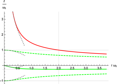
Figure 1: Roots of characteristic polynomial. Solid red: $\zeta_{2}=1/\tau-2u=\omega_{0}[(\tau\omega_{0})^{-1}+(\tau\omega_{0})-2(\tau\omega_{0})^{3}+\dots]>0$. Solid green: $\Re[\zeta_{1,3}]=-\omega_{0}[(\tau\omega_{0})/2-(\tau\omega_{0})^{3}+\dots]<0$. Dashed green: $\Im[\zeta_{1}]=\omega_{0}[1-5(\tau\omega_{0})^{2}/8+\dots]>0$, $\Im[\zeta_{3}]=-\Im[\zeta_{1}]$. Dashed gray: small–$(\tau\omega_{0})$ asymptotes. Grid lines mark $\Im[\zeta_{1,2}]$ extrema at $(\tau\omega_{0}=0,v/\omega_{0}=\pm 1)$, and $\Re[\zeta_{1,3}]$ minimum at $(\tau\omega_{0}=2,\,u/\omega_{0}=-1/4)$.

Denoting by $\zeta_{1},\,\zeta_{2},\,\zeta_{3}$ the roots of the characteristic polynomial associated with Eq. (23),

$$\zeta^{2}-\tau\zeta^{3}+\omega_{0}^{2}=0\;,$$ (27)

one finds, as expected for the roots of a $3^{\rm rd}$ order polynomial, a pair of complex–conjugate besides a real root,

$$\zeta_{1}=u+{\rm i}v\;,~{}~{}~{}~{}~{}\zeta_{2}=\frac{1}{\tau}-2u\;,~{}~{}~{}~{}~{}\zeta_{3}=u-{\rm i}v$$ (28)

with real and imaginary parts of $\zeta_{1}$ given by

$$u = -\frac{\left(w-1\right)^{2}}{6\tau w}\leq 0\;,~{}~{}~{}~{}~{}~{}~{}~{}v=\frac{1-w^{2}}{2\tau w\sqrt{3}}\geq 0\;,$$

$$w = \left[1+\frac{3}{2}\tau\omega_{0}\left(9\tau\omega_{0}-\sqrt{12+81\tau^{2}\omega_{0}^{2}}\right)\right]^{\frac{1}{3}}\;,$$ (29)

where $0\leq w\leq 1$. Real and imaginary parts of the characteristic–polynomial roots in Eq. (28) are displayed in Fig. 1 as function of the parameter $\tau\omega_{0}$.

III.3 Absence of AL steady–state solution

It is important to realize that the positive root $\zeta_{2}$ (red line in Fig. 1) implies a unique solution $x_{\rm AL}(t,t_{0})$ which will diverge in the steady–state limit,

$$\xi_{\rm AL}(t)=\lim_{t_{0}\to-\infty}x_{\rm AL}(t,t_{0})=\infty\;,$$ (30)

for generic initial conditions (see Appendix for details). Evidently, a steady–state solution of the AL equation does not, in general, exist. Facing this staggering fact, one must admit that Eq. (23) is not suited to model the steady–state elongation of a bounded atomic electron. This conclusion is corroborated by closer inspection of the special case, $f(t)\equiv 0$:

$$\ddot{x}(t)-\tau\dddot{x}(t)+\omega_{0}^{2}x(t)=0\;.$$ (31)

Introducing abbreviations

$$\Gamma=-2u\;,~{}~{}~{}~{}~{}~{}~{}\Omega^{2}=u^{2}+v^{2}\;,$$ (32)

the general solution of the homogeneous AL equation, Eq. (31), may be cast into the form ($t\geq t_{0}$)

$$x_{\rm AL}^{\rm h}(t,t_{0}) = \phi(t-t_{0})x_{0}+{\rm i}\chi(t-t_{0})mv_{0}$$

$$+{\rm e}^{(t-t_{0})\zeta_{2}}\left[b_{0}+\Gamma v_{0}+\Omega^{2}x_{0}\right]t_{1}^{2}(t,t_{0})\;,$$

which explicitly shows the contribution that will diverge, due to $\zeta_{2}>0$, when $(t-t_{0})$ grows large. That holds, because $t_{1}^{2}(t,t_{0})$ abbreviates an expression, which reduces to the positive constant $t_{1}^{2}(t,-\infty)=\tau^{2}/(1+4v^{2}\tau^{2})$ in the steady–state limit, while $\phi$ and $\chi$ denote relaxation and response function, resp., defined in Eq. (4) (or Eq. (8), equivalently) —for parameters ($\Gamma$, $\Omega^{2}$) provided in Eq. (32). Hence, the first line on r.h.s. of Eq. (III.3), which evidently represents the general homogeneous–equation solution of Eq. (1), will vanish in the steady–state limit.

An interesting aspect of the ‘run–away solution’ Eq. (III.3) is the observation that the diverging contribution would have been absent, if one assumed initial values not chosen independently as in Eq. (26) but in such a way that the pre–factor of ${\rm e}^{(t-t_{0})\zeta_{2}}$ in brackets on the r.h.s. of Eq. (III.3) will vanish,

$$\ddot{x}(t_{0})+\Gamma\dot{x}(t_{0})+\Omega^{2}x(t_{0})=0\;,$$ (34)

with $\Gamma=\Gamma(\tau,\omega_{0})$ and $\Omega^{2}=\Omega^{2}(\tau,\omega_{0})$ given in Eq. (32). This condition will prevent the solution of Eq. (31) from running away, —a noteworthy observation, because any instant of time could have been chosen to play the role of initial time $t_{0}$. I conclude:

1. Equation (34) must hold at any time $t$, if bounded elongations of the Lorentz–atom electron are to be guaranteed.

2. The equation of forced oscillations (Eq. (1) and properties discussed in Sec. II) with parameters

   $$\Gamma = -2u$$

   $$= \tau\omega_{0}^{2}\left[1-2(\tau\omega_{0})^{2}+{\cal O}\left((\tau\omega_{0})^{4}\right)\right]\;,$$

   $$\Omega = \sqrt{u^{2}+v^{2}}$$ (35)

   $$= \omega_{0}\left[1-(\tau\omega_{0})^{2}/2+{\cal O}\left((\tau\omega_{0})^{4}\right)\right]$$

   should be used for treating the Lorentz atom.

3. My conclusions are corroborated by the fact that the suggested procedure is consistent with the small–$\tau$ expansion given in Eq. (25).

III.4 Lorentz–atom polarizability

Following the conclusion of Sec. III.3 - item 2, the atomic dipole moment $d(t)=(-e)\xi(t)$, which is induced by the electric field of a standing light wave exerting the force $f(t)=(-e)E_{0}\cos(\omega t)$ on the electron (within dipole approximation), can be read from Eq. (19),

$$d(t)=\Re[\tilde{\chi}(\omega+{\rm i}o)e^{2}\,E_{0}{\rm e}^{-{\rm i}t\omega}]$$ (36)

with oscillator parameters

$$\Omega\to\omega_{0}\;,~{}~{}~{}~{}~{}~{}~{}~{}~{}\Gamma\to\tau\omega_{0}^{2}$$ (37)

taken from Eq. (2) —with perfectly sufficient precision in consideration of $\tau\omega_{0}\approx 10^{-8}$. The Lorentz model also allows to account for additional damping processes besides radiative loss by replacing $\Gamma$ in Eq. (36) with a total damping constant $\Gamma_{\rm t}$,

$$\Gamma\to\Gamma_{\rm t}=\Gamma+\Gamma^{\prime}\;,$$ (38)

which, as opposed to (jac:62, , Eq. (17.61)), does not depend on frequency.

In view of the constant dipole moment $d(t)=d_{0}$ induced by a static field $E_{0}$,

$$d_{0}=(\tilde{\chi}_{0}e^{2})\,E_{0}=\alpha E_{0}~{}~{}~{}~{}~{}~{}~{}~{}~{}(\omega=0)$$ (39)

with $\alpha=\tilde{\chi}_{0}e^{2}$ denoting the (static) polarizability, it has become common to name the dynamical dipole susceptibility, $\tilde{\alpha}(\omega+{\rm i}o)=\tilde{\chi}(\omega+{\rm i}o)e^{2}$, the “complex polarizability” (gwo:00, , Sec. II.A). Its real part, the (generalized $\omega$–dependent) polarizability

$$\alpha(\omega)=\Re[\tilde{\alpha}(\omega+{\rm i}o)]=\chi^{\prime}(\omega)e^{2}\;,$$ (40)

determines a force ${\bf F}{\!\,=\,\!}-\vec{\nabla}U_{\rm dip}$ acting on the atom in the light field, where

$$U_{\rm dip}({\bf r})=-\frac{1}{2}\alpha(\omega)\overline{|{\bf E}({\bf r},t)|^{2}}=-\chi^{\prime}(\omega)e^{2}\frac{E_{0}^{2}}{4}$$ (41)

denotes the ‘optical dipole potential’ which will be identified as the average atomic energy shift, known as ‘ac–Stark effect’ in Sec. IV.5 below. Within classical electrodynamics, the optical dipole potential can only be made plausible to within a factor 2, because one has $-\overline{{\bf d}(t)\cdot{\bf E}_{0}\cos(\omega t)}=-\chi^{\prime}(\omega)e^{2}E_{0}^{2}/2$ for the time–averaged potential energy of an electric dipole moment in an external electric field.

III.5 Absorption and scattering of radiation by Lorentz atom

The imaginary part of the dynamical dipole susceptibility, $\Im[\tilde{\alpha}(\omega+{\rm i}o)]=\chi^{\prime\prime}(\omega)e^{2}$, via Eq. (22) determines the average power $P(\omega)$ absorbed by the atom from the electric field, which implies the absorption cross–section ($\lambdabar_{0}=c/\omega_{0}$, wavelength at resonance, divided by $2\pi$),

$$\sigma_{\rm abs}(\omega)=\frac{P(\omega)}{\epsilon_{0}cE_{0}^{2}/2}=6\pi\lambdabar_{0}^{2}\frac{\Gamma\Gamma_{\rm t}\omega^{2}}{\left(\omega_{0}^{2}-\omega^{2}\right)^{2}+\left(\omega\Gamma_{\rm t}\right)^{2}}$$ (42)

which obeys the famous $f$–sum rule,

$$\int_{0}^{\infty}{\!\rm d}\omega~{}\sigma_{\rm abs}(\omega)~{}=\frac{\pi}{2\epsilon_{0}c}\frac{e^{2}}{m}\;,$$ (43)

also known as ‘dipole sum rule’ in the present context. It must be emphasized that the $f$-sum rule, valid for both classical and quantum mechanical systems, states the following interesting fact. The integrated absorption cross section on the r.h.s. of Eq. (43) is determined by the ratio $e^{2}/m$ alone. It does not depend on further details of the system, here represented by oscillator frequency and damping constants.

A photon-absorption rate $\Gamma_{\rm abs}(\omega)$ has been considered in (gwo:00, , Sec. II.A) which is determined by $\chi^{\prime\prime}(\omega)$, too. From quantum–mechanical scattering theory, one finds ($\Theta(x)$ denoting unit–step function)

$$\Gamma_{\rm abs}(\omega)=\frac{\chi^{\prime\prime}(\omega)}{2\hbar}\,e^{2}E_{0}^{2}~{}\Theta(\omega)=\frac{P(\omega)}{\hbar\omega}~{}\Theta(\omega)\;,$$ (44)

if the atom is assumed in its electronic ground state (i. e., at zero temperature) when hit by photons. In Eq. (44), $\Gamma_{\rm abs}(-\omega)=0$ for $\omega>0$ expresses the fact that an atom in its ground state cannot loose energy by stimulated (or spontaneous) emission of a photon of energy $\hbar\omega$. It can only win energy by absorbing a photon of energy $\hbar\omega$.

Finally, the time–dependent dipole moment induced by the oscillatory external field (Eq. (36)) will produce an electromagnetic field which in the far–field dipole–approximation $({\bf E},{\bf B})_{\rm rad}=\frac{\ddot{d}(t-r/c)}{4\pi\epsilon_{0}c^{2}r}\left[{\bf e}\times\frac{{\bf r}}{r}\right]\left(\times\frac{{\bf r}}{r},\,\frac{1}{c}\right)$ may be interpreted in terms of a radiation–scattering cross section (gaf:10, , Eq. (2A.48)), (jac:62, , Eq. (17.63))

$$\sigma_{\rm sc}(\omega) = \frac{8\pi}{3}R^{2}\frac{\omega^{4}}{\left(\Omega^{2}-\omega^{2}\right)^{2}+\left(\omega\Gamma_{\rm t}\right)^{2}}$$ (45)

$$\to 6\pi\lambdabar_{0}^{2}\left(\frac{\Gamma}{\omega_{0}}\right)^{2}\left\{\begin{array}[]{cl}\omega^{4}/\omega_{0}^{4}&,\,\omega\ll\omega_{0}\\ \frac{(\omega_{0}/2)^{2}}{(\omega-\omega_{0})^{2}+(\Gamma_{\rm t}/2)^{2}}&,\,\omega\approx\omega_{0}\\ 1&,\,\omega\gg\omega_{0}\end{array}\right.$$ (49)

from which well–known scattering regimes are easily identified as limiting cases: Rayleigh scattering for $\omega\ll\Omega$, Thomson scattering for $\omega\gg\Omega$, and, for $\omega\approx\Omega$, the resonant Lorentz scattering exhibiting the characteristic line shape with ‘full width at half maximum (FWHM)’, $\Gamma_{\rm t}$, and ‘peak cross section’,

$$\sigma_{\rm sc}(\Omega)=\frac{8\pi}{3}R^{2}\frac{\Omega^{2}}{\Gamma_{\rm t}^{2}}=6\pi\lambdabar_{0}^{2}\,\left(\frac{\Gamma}{\Gamma_{\rm t}}\right)^{2}\;.$$ (50)

Here $R=3c\tau/2$ denotes the classical electron radius, and oscillator parameters are given by $\Omega=\omega_{0}$ and total decay constant $\Gamma_{\rm t}=\Gamma+\Gamma^{\prime}$ with $\Gamma=\tau\omega_{0}^{2}$.

As opposed to the statement in (jac:62, , Eq. (17.72)) which refers to all $\omega$, Eqs. (42) and (45) imply $\sigma^{\rm L}_{\rm abs}(\omega)=\sigma^{\rm L}_{\rm sc}(\omega)+\sigma^{\rm L}_{\rm r}(\omega)$ for frequencies $|\omega-\omega_{0}|\ll\omega_{0}$ only, i. e., for the resonant Lorentz–absorption (or total) cross section. The total cross section is composed of a scattering contribution $\sigma^{\rm L}_{\rm sc}(\omega)$, spelled out in Eq. (45) ($\omega\approx\omega_{0}$), and a ‘reaction cross section’ $\sigma^{\rm L}_{\rm r}(\omega)$ with the same Lorentz resonance denominator, but $\Gamma$ replaced with $\sqrt{\Gamma\Gamma^{\prime}}$ in the numerator. Consequently, $\sigma^{\rm L}_{\rm abs}(\omega)$ must be given by $\sigma^{\rm L}_{\rm sc}(\omega)$ with $\Gamma$ replaced by $\sqrt{\Gamma\Gamma_{\rm t}}$ in the numerator, which is easily verified from Eq. (42). The reason for the discrepancy with Ref. jac:62 will become clear in Sec. III.6.

III.6 Pitfalls

Regarding the classical model of the atomic complex polarizability, much confusion has been created in literature by erroneous conclusions drawn from the AL equation of motion, Eq. (23), with oscillatory external force $f(t)=f_{0}\cos(\omega t)$. In Refs. jac:62 , gri:99 , gwo:00 , gaf:10 , e. g., and in numerous other publications, authors search for a particular solution of Eq. (23) which oscillates with frequency $\omega$ of the driving force. Indeed, there is one such solution,

$$x^{\rm osc}(t)=\frac{(\omega_{0}^{2}-\omega^{2})\cos(\omega t)+\tau\omega^{3}\sin(\omega t)}{(\omega_{0}^{2}-\omega^{2})^{2}+(\tau\omega^{3})^{2}}\frac{f_{0}}{m}\;,$$ (51)

which can be checked easily by inserting $x^{\rm osc}(t)$ into Eq. (23). But $x^{\rm osc}(t)$ is not the steady–state solution of the inhomogeneous AL equation. According to Eq. (30), such a steady–state solution does not exist which brought me to rule out the AL equation of motion as a candidate for describing the Lorentz–atom elongation.

It must be emphasized that, in contrast to my findings, Eq. (51) is frequently claimed to present the steady–state solution to the AL equation with oscillatory force, which is not true as I demonstrated in Sec. III.3. Since $x^{\rm osc}(t)$ is not the steady–state solution, we are not allowed to interpret Eq. (51) as if it were the analog of Eq. (19). Extracting from Eq. (51) a “susceptibility”,

$$X(\omega)=\frac{\omega_{0}^{2}}{\omega_{0}^{2}-\omega^{2}-{\rm i}\tau\omega^{3}}X_{0}\;,~{}~{}~{}~{}~{}~{}~{}X_{0}=\frac{1}{m\omega_{0}^{2}}$$ (52)

is a frequently repeated mistake which

• is found already in the high–impact monograph jac:62 , where in (jac:62, , Eqs. (17.60-61)) a non–radiative decay constant $\Gamma^{\prime}$ was assumed in addition to the radiative decay constant $\Gamma=\tau\omega_{0}^{2}$, both of which were combined into a total decay constant $\Gamma_{\rm t}(\omega)=\Gamma^{\prime}+(\omega/\omega_{0})^{2}\Gamma$, which is evidently not constant! Moreover, $\Gamma_{\rm t}(\omega)$ violates the $f$–sum rule and suppresses the high–frequency Thomson scattering in (jac:62, , Eq. (17.63)). According to my findings in Eqs. (2–36), the total decay rate must here read $\Gamma_{\rm t}=\Gamma^{\prime}+\Gamma$ as arrived at in Eq. (38) above, which will repair the mentioned deficiencies.

• was made in the monograph (gri:99, , Ex. 11.4, p. 468) implicitly, when claiming $\Gamma=\tau\omega^{2}$ instead of the correct result Eq. (2),

• has been carried on into the optical–dipole potential community by the very informative and often cited review article (gwo:00, , Sec. II. A),

• is even found in the more recent monograph gaf:10 , where it shows up in (gaf:10, , Eq. (2A.53)) and again, as a nasty suppressor of Thomson scattering, in (gaf:10, , Eq. (2A.48)).

• would also result, if one erroneously applied to Eq. (23) the mnemonic trick which is so helpful in remembering $\tilde{\chi}(\omega+{\rm i}o)$.

  Namely, Fourier transforming Eq. (1) which is, of course, obeyed by the steady–state elongation $\xi(t)$,

  $$m\left[(-{\rm i}\omega)^{2}+(-{\rm i}\omega)\Gamma+\Omega^{2}\right]\xi_{\omega}=f_{\omega}$$

  $$=\left[\tilde{\chi}(\omega+{\rm i}o)\right]^{-1}\xi_{\omega}\;,$$ (53)

  and reading the result Eq. (12) for $\tilde{\chi}(\omega+{\rm i}o)$ from the Fourier–transformed equation of motion.

  Note that the “short–cut” Eq. (• ‣ III.6) works out alright only, because I proved in Sec. II.2 above that Eq. (1) does indeed have a unique steady–state solution. The same, however, does not hold true for the AL equation (Eq. (23)) as I demonstrated in Sec. III.3 above.

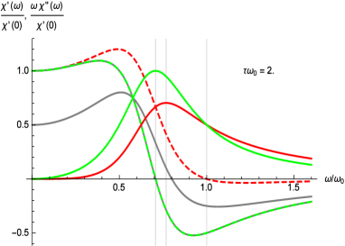
Figure 2: Kramers–Kronig check. Full green: $\omega\chi^{\prime\prime}(\omega)/\tilde{\chi}_{0}$ (Eq. (14)); dashed green: $\chi^{\prime}(\omega)/\tilde{\chi}_{0}$ (Eq. (13)); full red: $\omega\Im[X(\omega)]/X_{0}$ (Eq. (52)); dashed red: $\Re[X(\omega)]/X_{0}$ (Eq. (52)); full gray: integrals on r.h.s. (Eq. (54) & first Eq. (87)). Grid lines indicate positions of $\Omega$, $\omega_{\rm m}^{X}$, $\omega_{0}$ (from left to right).

But why can $X(\omega)$ not serve as a proper dynamical susceptibility, anyway? Answer: Because it does not obey Kramers–Kronig relations,

$$\Re[X(\omega)]\neq\frac{1}{\pi}-\!\!\!\!\!\!\!\int_{-\infty}^{\infty}{\!\rm d}\bar{\omega}~{}\frac{\Im[X(\bar{\omega})]}{\bar{\omega}-\omega}\;,$$ (54)

which is a consequence of $x^{\rm osc}(t)$ not being the steady–state solution of the AL equation. Inequality Eq. (54) is clearly demonstrated in Fig. 2, where the full gray line (cutting the ordinate at $\approx 0.5$) displays the numerically evaluated principal–value integral from r.h.s. of Eq. (54) which has been divided by the constant $X_{0}$. This should be compared with $\Re[X(\omega)]/X_{0}$ depicted as dashed red line. Both curves differ markedly indicating violation of the Kramers–Kronig relation. As pointed out above, however, a proper susceptibility must obey this relation. As opposed to $X(\omega)$, the real and imaginary parts of the dynamical susceptibility in Eq. (12) do form a Kramers–Kronig pair. This has also been demonstrated in Fig. 2: the gray line representing the numerically evaluated principal–value integral (first Eq. (87) for $f^{\prime\prime}(\omega)\to\chi^{\prime\prime}(\omega)$, after dividing by $\tilde{\chi}_{0}$) cannot be distinguished from the dashed green line displaying $\chi^{\prime}(\omega)/\tilde{\chi}_{0}$ from Eq. (13). The very large parameter value chosen in Fig. 2 for demonstration purposes, $\tau\omega_{0}=2$, requires exact evaluation of $\Gamma$ and $\Omega^{2}$ using Eq. (32) with Eq. (III.2).

The difference between correct (green) and faulty (red) model polarizability curves will diminish for decreasing values of $\tau\omega_{0}$. This observation is substantiated by the relations

$$\frac{\Re[\tilde{X}(\omega)]}{\chi^{\prime}(\omega)} = 1-(\tau\omega_{0})^{2}\left\{1-\frac{\omega^{4}\left[1+{\cal O}\left((\tau\omega_{0})^{2}\right)\right]}{(\omega_{0}^{2}-\omega^{2})\omega_{0}^{2}}\right\}$$

$$\frac{\Im[\tilde{X}(\omega)]}{\chi^{\prime\prime}(\omega)} = \frac{\omega^{2}}{\omega_{0}^{2}}~{}\left\{1-(\tau\omega_{0})^{2}\frac{\omega^{2}\left[1+{\cal O}\left((\tau\omega_{0})^{2}\right)\right]}{\omega_{0}^{2}}\right\}$$

found from comparison of Eq. (52) with Eqs. (13–14), where $\Gamma$ and $\Omega$ are given in Eq. (2). For electron parameters ($\tau\omega_{0}\approx 10^{-8}$), it seems that use of the incorrect $\tilde{X}(\omega)$ will produce quantitatively acceptable polarizability results, if one restricts to the frequency range

$$1\gg\left|1-\frac{\omega^{2}}{\omega_{0}^{2}}\right|\gg(\tau\omega_{0})^{2}$$ (57)

which allows to set $\omega^{2}/\omega_{0}^{2}\approx 1$ in Eq. (III.6) and, at the same time, keep sufficient distance to the pole in Eq. (III.6).

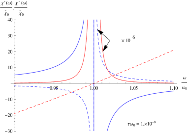
Figure 3: Polarizability: reactive (blue) and dissipative (red, $10^{6}$–fold amplified) parts. Errors from Eqs. (III.6),(III.6): $\{\Re[X(\omega)]/\chi^{\prime}(\omega)-1\}\times 10^{2}$ (blue–dashed, $10^{6}$–fold amplified) and $\{\Im[X(\omega)]/\chi^{\prime\prime}(\omega)-1\}\times 10^{2}$ (red–dashed) reflecting factor $\omega^{2}/\omega_{0}^{2}$ in Eq. (III.6).

The limitations imposed on the range of frequencies by Eq. (57) are best appreciated by throwing a glance at Fig. 3, where relative errors derived from Eqs. (III.6–III.6) are displayed together with $\chi^{\prime}(\omega)$ and $\chi^{\prime\prime}(\omega)$ for the realistic value $\tau\omega_{0}=10^{-8}$ referring to the oscillating electron of the Lorentz atom. From Fig. 3 it is clear that big quantitative errors ($\pm$20% for $|\omega/\omega_{0}-1|\approx 0.1$) only occur in the imaginary part and in a detuning range, where $\chi^{\prime\prime}(\omega)$ is very small, while the quantitative error in the real part is negligibly small in magnitude ($<3.\times 10^{-5}$ % for $|\omega/\omega_{0}-1|>0.005$).

On the one hand, this observation may possibly explain, why the analytically incorrect polarizability $X(\omega)$ (Eq. (52)) could survive in literature for so long without being debunked.

On the other hand, Fig. 3 clearly demonstrates that the photon–absorption rate $\Gamma_{\rm abs}(\omega)$ deduced from Eq. (52) is systematically under– (over–)estimating the true photon–absorption rate in the red– (blue–)detuned frequency regime (see, e.g., in (gwo:00, , Eqs. (11),(41))). For the experimentally relevant ratio of absorption rate and optical dipole potential (cf. (gwo:00, , Eq. (14))), one finds from Eqs. (44),(22) the simple result,

$$\frac{\hbar\Gamma_{\rm abs}}{U_{\rm dip}}=\frac{2\omega\Gamma}{\omega^{2}-\Omega^{2}}=\left\{\begin{array}[]{rl}-2\omega\Gamma/\Omega^{2}&\left[1+{\cal O}\left(\omega^{2}/\Omega^{2}\right)\right]\\ \Gamma/\Delta&\left[1+{\cal O}\left(\Delta/\Omega\right)\right]\end{array}\right.$$ (58)

where $\Delta=\omega-\Omega$ and $\omega\geq 0$. For a “quasi–electrostatic trap” (QUEST), this ratio is under–estimated by roughly $100$% (for $\omega\ll\Omega$), because $\Gamma_{\rm abs}$ will be larger by the factor $(\Omega/\omega)^{2}$ if deduced from Eq. (52). For a “far off–resonance trap” (FORT), which is understood to be detuned sufficiently slightly to still obey $|\Delta|\ll\Omega$, the incorrect polarizability happens to produce the correct ratio $\Gamma/\Delta$ given in Eq. (58), because $\omega\approx\Omega$.

IV Quantum–mechanical reasoning

IV.1 Perturbation expansion for expectation value

A physical system (Hamiltonian $\hat{H}$) will take on the explicitly time–dependent Hamiltonian

$$\hat{H}_{t}=\hat{H}-\hat{D}E_{0}\cos(\omega t)$$ (59)

under the influence of an external, linearly polarized, oscillatory field ${\bf e}E_{0}\cos(\omega t)$ which couples to the dynamical variable $\hat{D}={\bf\hat{D}\cdot e}$. As a consequence, the average value at time $t$ of an arbitrary operator $\hat{O}_{t}$ will deviate from its stationary–state value,

$$\left\langle\,\delta\hat{O}_{t}\,\right\rangle_{t} \equiv \left\langle\,\hat{O}_{t}\,\right\rangle_{t}-\left\langle\,\hat{O}_{t}\,\right\rangle$$ (60)

$$= \left\langle\,\hat{O}_{t}\,\right\rangle_{t}^{(1)}+\left\langle\,\hat{O}_{t}\,\right\rangle_{t}^{(2)}~{}+~{}\dots\;.$$

Assuming the perturbing field switched on adiabatically at time $t_{0}=-\infty$ (which amounts to replacing $E_{0}\cos(\omega t^{\prime})\to{\rm e}^{-o(t-t^{\prime})}E_{0}\cos(\omega t^{\prime})$ with $o>0$ for all $t^{\prime}\leq t$), the $n$–th order in $E_{0}$ contribution to $\left\langle\,\delta\hat{O}_{t}\,\right\rangle_{t}$ reads explicitly ($\tau_{0}=0$),

$$\left\langle\,\hat{O}_{t}\,\right\rangle_{t}^{(n)} = {\rm i}^{n}\int_{\tau_{0}}^{\infty}{\!\rm d}\tau_{1}\dots\int_{\tau_{n-1}}^{\infty}{\!\rm d}\tau_{n}~{}\chi_{\hat{O}_{t}^{\dagger};\hat{D}}(\tau_{1},\dots,\tau_{n})$$ (61)

$$\hskip 30.00005pt\times\prod_{j{\!\,=\,\!}1}^{n}{\rm e}^{-o\tau_{j}}E_{0}\cos[\omega(t-\tau_{j})]$$

with the $n$–th order response function,

$$\chi_{\hat{A};\hat{B}}(\tau_{1},\dots,\tau_{n})=$$ (62)

$$\frac{1}{\hbar^{n}}\left\langle\,\left[\dots\left[\left[\hat{A}^{\dagger}\,,\,\hat{B}(-\tau_{1})\right]\,,\,\hat{B}(-\tau_{2})\right]\dots\,,\,\hat{B}(-\tau_{n})\right]\,\right\rangle.$$

Here $\hat{B}(t)=\exp({\rm i}t\hat{H}/\hbar)\hat{B}\exp(-{\rm i}t\hat{H}/\hbar)$ denotes a Heisenberg operator referring to the unperturbed system, and the stationary–state average is defined as

$$\left\langle\,\hat{A}\,\right\rangle={\rm Tr}\left\{\hat{A}\hat{W}\right\}\;,~{}~{}~{}~{}\left[\hat{H}\,,\,\hat{W}\right]=0$$ (63)

with statistical operator $\hat{W}$ describing the initial stationary state of the unperturbed system.

It must be emphasized that $\left\langle\,\delta\hat{O}_{t}\,\right\rangle_{t}$ in Eqs. (60–62) describes the steady–state deviation from the unperturbed expectation value, which is induced by the external field. Interestingly enough, the first–order result $\left\langle\,\hat{O}_{t}\,\right\rangle_{t}^{(1)}$ (written out explicitly in Eq. (64) for the induced dipole moment) has the same structure found for the steady–state solution in Eq. (9) for the classical oscillator elongation.

IV.2 Induced dipole moment

For the atomic dipole moment induced by a linearly–polarized standing light wave of frequency $\omega$, one reads for the first–order result $d(t)=\left\langle\,\delta\hat{D}\,\right\rangle_{t}^{(1)}$ from Eq. (61),

$$d(t) = {\rm i}\int_{0}^{\infty}{\!\rm d}\tau~{}{\rm e}^{-o\tau}\chi_{\hat{D};\hat{D}}(\tau)E_{0}\cos[\omega(t-\tau)]$$ (64)

$$= \Re\left[\tilde{\chi}_{\hat{D};\hat{D}}(\omega+{\rm i}o)E_{0}{\rm e}^{-{\rm i}\omega t}\right]\;,$$

with the dipole–dipole response function

$$\chi_{\hat{D};\hat{D}}(t)=\frac{1}{\hbar}\left\langle\,\left[\hat{D}(t)\,,\,\hat{D}\right]\,\right\rangle=-\chi_{\hat{D};\hat{D}}(-t)\;,$$ (65)

where $\hat{D}$ is identified with the component in field direction of the atomic dipole–moment operator ${\bf\hat{D}}$.

The corresponding dynamical dipole–susceptibility (“complex polarizability”) resulting from Fourier–Laplace transforming $\chi_{\hat{D};\hat{D}}(t)$ according to Eq. (85), may quite generally be cast into the form mar:68

$$\tilde{\chi}_{\hat{D};\hat{D}}(z) = \frac{\Omega_{D}^{2}}{\Omega_{D}^{2}-z^{2}-z\tilde{K}_{D}(z)}\,\tilde{\chi}_{\hat{D};\hat{D}}({\rm i}o)\;.$$ (66)

This formally exact expression is cited here only to point out the following facts.

• The relaxation kernel $\tilde{K}_{D}(z)=\int_{-\infty}^{\infty}\frac{{\!\rm d}\overline{\omega}}{\pi}\frac{K_{D}^{\prime\prime}(\overline{\omega})}{\overline{\omega}-z}$ is determined by an even, non–negative, and bounded spectral function $K_{D}^{\prime\prime}(\omega)$. This generally frequency–dependent ‘total damping constant’ $K_{D}^{\prime\prime}(\omega)=\Im[\tilde{K}_{D}(\omega+{\rm i}o)]$ will inevitably be associated with a resonance–frequency renormalization via $\Re[\tilde{K}_{D}(\omega+{\rm i}o)]$. Such a real contribution is missing in (jac:62, , Eq. (17.60)) resulting in the violation of Kramers–Kronig relations and $f$–sum rule discussed in Sec. III.6 above. Moreover, $\Gamma_{\rm t}(\omega)$ in (jac:62, , Eq. (17.61)) is not bounded.

• The relaxation kernel $\tilde{K}_{D}(z)$ is the FLT of the dipole memory function $K_{D}(t)$ governing the generalized oscillator equation,

  $$\ddot{\phi}_{\hat{D};\hat{D}}(t)+\Omega_{D}^{2}\phi_{\hat{D};\hat{D}}(t)+\int_{0}^{t}{\!\rm d}t^{\prime}K_{D}(t^{\prime})\dot{\phi}_{\hat{D};\hat{D}}(t-t^{\prime})=0$$ (67)

  with initial conditions $\phi_{\hat{D};\hat{D}}(0)=1$, $\dot{\phi}_{\hat{D};\hat{D}}(0)=0$, which is obeyed by the (normalized) dipole relaxation function. Both, Eq. (66) and Eq. (67), are formally exact and, in view of Kubo’s identity Eq. (16), equivalent statements.

To conclude these general remarks, I emphasize that memory effects may be neglected in some applications, rendering

$$K_{D}(t)\approx 2\Gamma\delta(t)\Longrightarrow K_{D}^{\prime\prime}(\omega)\approx\Gamma\Longrightarrow\tilde{K}_{D}(z)\approx s{\rm i}\Gamma$$ (68)

a reasonable approximation —as is the case for the quantum oscillator in Sec. IV.3. Under these circumstances, Eq. (67) reduces to a free–oscillations equation of the same type obeyed by the classical relaxation function $\phi(t)$ introduced in Sec. II. These remarks on very general quantum mechanical (and quantum statistical) results may illuminate the great success of models such as the Lorentz atom, which are based on the classical forced–oscillations equation of motion.

IV.3 Quantum oscillator

Assuming the eigenvalue problem of the unperturbed Hamiltonian solved ($\hat{H}\,|\,n\,\rangle=\,|\,n\,\rangle\varepsilon_{n}$, $n=0,1,2,\dots$) and the atom in its ground state initially ($\hat{W}=\,|\,0\,\rangle\langle\,0\,|\,$), the dipole–response function defined in Eq. (65) is easily evaluated,

$$\chi_{\hat{D};\hat{D}}(t)=\frac{2}{{\rm i}\hbar}\sum_{n\neq 0}\left|D_{n0}\right|^{2}\sin(\omega_{n0}t)~{}{\rm e}^{-\frac{\Gamma_{n}}{2}|t|}\;,$$ (69)

with the dynamical susceptibility,

$$\tilde{\chi}_{\hat{D};\hat{D}}(z)=\sum_{n\neq 0}\frac{2m\omega_{n0}}{\hbar e^{2}}\left|D_{n0}\right|^{2}\frac{\Omega_{n}^{2}\,\tilde{\chi}_{n}({\rm i}o)}{\Omega_{n}^{2}-z^{2}-s{\rm i}\Gamma_{n}z}\;,$$ (70)

given by Fourier–Laplace transformation. Here $D_{n0}=\langle\,n\,|\,{\bf\hat{D}}\cdot{\bf e}\,|\,0\,\rangle$ are dipole–moment matrix elements and $\omega_{n0}=(\varepsilon_{n}-\varepsilon_{0})/\hbar$ denote atomic excitation frequencies ($n{\!\,=\,\!}1,2,\dots$). Abbreviations have been introduced for partial static polarizabilities and resonance frequencies, $\tilde{\chi}_{n}({\rm i}o)=e^{2}/(m\Omega_{n}^{2})$ and $\Omega_{n}^{2}=\omega_{n0}^{2}+(\Gamma_{n}/2)^{2}$, respectively.

In Eq. (69), ad–hoc damping factors have been inserted which account approximately for the natural lifetimes of excited atomic states while preserving the symmetry spelled out in Eq. (65). Excited atomic states are well known to have a finite natural lifetime $\tau_{n}=1/\Gamma_{n}$ even if no electromagnetic field is applied, because there is “spontaneous emission” due to the atom interacting with vacuum fluctuations, interactions which have not been included into the unperturbed Hamiltonian $H$. In leading order (electric dipole transitions), spontaneous emission will occur at a rate (hei:53, , Chap. V)

$$\Gamma_{n}=\frac{4\alpha}{3c^{2}}\sum_{n^{\prime}}^{\varepsilon_{n^{\prime}}<\varepsilon_{n}}\omega_{nn^{\prime}}^{3}\left|\langle\,n^{\prime}\,|\,{\bf\hat{r}}\,|\,n\,\rangle\right|^{2}\;,$$ (71)

where $\alpha=e^{2}/(4\pi\epsilon_{0}~{}\hbar c)\approx 1/137$ denotes the Sommerfeld fine–structure constant.

It is very instructive to evaluate the dipole–response function in detail for a simple model of an atom. Within the quantum–oscillator model for the atomic electron, $\hat{H}=\hbar\omega_{10}(\hat{a}^{\dagger}\hat{a}+1/2)$, one has for the electric dipole–moment operator $\hat{D}=-ex_{0}(\hat{a}^{\dagger}+\hat{a})$ with oscillator length $x_{0}=\sqrt{\hbar/(2m_{\rm e}\omega_{10})}$ resulting in matrix elements $\left|D_{n0}\right|^{2}=e^{2}x_{0}^{2}~{}\delta_{n,1}$, which leave only a single term in the sum on r.h.s of Eq. (69),

$$\chi_{\hat{D};\hat{D}}(t)=e^{2}\frac{\sin(\omega_{10}t)}{{\rm i}m_{\rm e}\omega_{10}}~{}{\rm e}^{-\frac{\Gamma_{1}}{2}|t|}\;.$$ (72)

Evaluation of the damping constant $\Gamma_{1}$ using the transition rate of Eq. (71) results in

$$\begin{array}[]{cccl}\omega_{10}&=&(E_{1}-E_{0})/\hbar&\longleftrightarrow~{}\tilde{\Omega}\\ \Gamma_{1}&=&\bar{\tau}\omega_{10}^{2}&\longleftrightarrow~{}\Gamma\end{array}\;,$$ (73)

where the characteristic time $\bar{\tau}$ turns out to be identical to the time constant $\tau$ introduced in Eq. (24),

$$\bar{\tau}\equiv\tau=\frac{2\alpha\hbar}{3m_{\rm e}c^{2}}\approx 6.3\times 10^{-24}\,{\rm s}\;.$$ (74)

The quantum–mechanical results derived above are noteworthy in several respects, as they demonstrate why the classical oscillator model discussed in Sec. II has been so extremely successful in describing an atom irradiated by light.

1. The general result Eq. (64) for the induced dipole moment of any physical system in a weak electric field has the same formal structure as one finds for the steady–state elongation of a classical oscillator subjected to an external field, see Eq. (9).

2. Dipole–dipole response function of a quantum oscillator (Eq. (72)) and elongation–response function of a classical oscillator (Eq. (8)) become identical —after multiplying the latter by $(-e)^{2}$ and identifying induced moment $(-e)x(t)\to\left\langle\,\delta\hat{D}\,\right\rangle_{t}$, force $f(t)\to(-e)E(t)$, and fixing oscillation frequency and damping constant of the classical Lorentz atom according to Eq. (73).

Note that the latter identification solves, by quantum–mechanical arguments, the problem of finding appropriate parameters $\Omega,\Gamma$ to be used for the classical Lorentz–atom: $\Omega=\omega_{10}\left[1+{\cal O}\left((\tau\omega_{10})^{2}\right)\right]$, $\Gamma=\tau\omega_{10}^{2}$, which to leading order in the small parameter $(\tau\omega_{10})$ agree with the classical solution, provided one also identifies $\hbar$ times the classical resonance frequency $\omega_{0}$ with the energy difference $(E_{1}-E_{0})$, i. e., $\omega_{0}\equiv\omega_{10}$.

Lorentz and Abraham at the end of 19^th century, of course, did not have recourse to results from quantum theory (cf. Eqs. (72–73)). They had to specify their model parameters by using classical electrodynamics, only. While $\Omega$ in Eq. (1) could naturally be associated with the frequency of resonantly absorbed light, determination of $\Gamma$ required introduction of a radiative reaction force which lead to the strange new AL equation of motion (Eq. (23)) for the oscillator elongation.

It is therefore noteworthy and comforting to see that the classical radiation–damping constant $\Gamma$ derived from AL equation (Eq. (2)) is perfectly reproduced by the quantum–mechanical result in Eq. (73).

IV.4 Average absorbed power

The average power absorbed from the external oscillatory field by the physical system described in Eq. (59) is given by

$$P(\omega) = \overline{{\frac{\rm d}{{\rm d}t}}{\left\langle\,H_{t}\,\right\rangle_{t}}}=\overline{\left\langle\,{\frac{{\partial}H_{t}}{{\partial}t}}\,\right\rangle_{t}}=\overline{\left\langle\,\delta\hat{D}\,\right\rangle_{t}\sin(\omega t)}E_{0}$$ (75)

$$= \frac{1}{2}\,\omega\chi^{\prime\prime}_{\hat{D};\hat{D}}(\omega)\,E_{0}^{2}~{}+~{}{\cal O}(E_{0}^{3})\;,$$

where $\overline{F(t)}=\frac{1}{T}\int_{0}^{T}{\!\rm d}t~{}F(t)$, $T=2\pi/\omega$ and, in the last line, use has been made of Eq. (64). The quantum–mechanical result in lowest non–vanishing order of perturbation theory, Eq. (75), should be compared to the classical expression Eq. (22). As in case of the induced dipole moment, the formal structures of both, quantum and classical, results for $P(\omega)$ are identical. The average power absorbed from the $ac$-electric field by a charged quantum oscillator in its ground state will coincide with the power absorbed by the classical oscillator, because of equivalent response functions, cf. Sec. IV.3 - item 2.

IV.5 $ac$–Stark effect and optical dipole potential

The energy $\left\langle\,H\,\right\rangle$ of an atom is expected to change upon applying an electric field $E_{0}\cos(\omega t)$. Such a phenomenon is well known as Stark shift in case of a constant electric field ($\omega=0$). Since an atom in its ground state has no permanent dipole moment, the Stark shift is typically of $2^{\rm nd}$ order in $E_{0}$. The rapidly oscillating electric field of visible light will also induce a shift of the atomic energy, which is rapidly oscillating with frequency $\omega$ and known as $ac$–Stark effect. Due to the high frequency of light, the induced shift cannot be detected by time–resolved measurements. Therefore, only the time–averaged shift is of interest here (averaging over period $T=2\pi/\omega$).

Applying the perturbation expansion Eq. (60) to the operator of total energy, $\hat{O}_{t}\to\hat{H}_{t}$, the averaged induced energy shift is

$$\overline{\left\langle\,\delta\hat{H}_{t}\,\right\rangle_{t}} = \overline{\left\langle\,\hat{H}_{t}\,\right\rangle_{t}}-\left\langle\,H\,\right\rangle=\Delta\varepsilon+{\cal O}(E_{0}^{3})\;,$$

$$\Delta\varepsilon = -E_{0}\overline{\left\langle\,\hat{D}\,\right\rangle_{t}^{(1)}\cos(\omega t)}+\overline{\left\langle\,\hat{H}\,\right\rangle_{t}^{(2)}}\;.$$ (76)

Since one may replace under the time average $\left\langle\,\hat{D}\,\right\rangle_{t}^{(1)}\to\left\langle\,\delta\hat{D}\,\right\rangle_{t}^{(1)}$, the first contribution to $\Delta\varepsilon$ is easily evaluated with the help of the induced dipole moment in Eq. (64),

$$-E_{0}\overline{\left\langle\,\hat{D}\,\right\rangle_{t}^{(1)}\cos(\omega t)}=-\chi^{\prime}_{\hat{D};\hat{D}}(\omega)\frac{E_{0}^{2}}{2}\;.$$ (77)

Here $\chi^{\prime}_{\hat{D};\hat{D}}(\omega)=\alpha(\omega)$ is the electric polarizability defined quantum–mechanically, which should be compared to its classical pendent in Eq. (40). The second contribution to $\Delta\varepsilon$ (Eq. (76)) is read from Eq. (61). Noting the relation

$$\chi_{\hat{H};\hat{D}}(\tau_{1},\tau_{2})=\frac{1}{{\rm i}}{\frac{{\partial}}{{\partial}\tau_{2}}}\chi_{\hat{D};\hat{D}}(\tau_{2}-\tau_{1})$$ (78)

between quadratic and linear dipole–dipole response function, and employing $\sin(\omega t)/t\to\pi\delta(t)$ for large $\omega$ under the final integral, one finds

$$\overline{\left\langle\,\hat{H}\,\right\rangle_{t}^{(2)}} = {\rm i}^{2}\int_{0}^{\infty}{\!\rm d}\tau_{1}\int_{\tau_{1}}^{\infty}{\!\rm d}\tau_{2}~{}\chi_{\hat{H};\hat{D}}(\tau_{1},\tau_{2})$$ (79)

$$\times{\rm e}^{-o(\tau_{1}+\tau_{2})}\cos[\omega(\tau_{2}-\tau_{1})]\frac{E_{0}^{2}}{2}$$

$$= \frac{{\rm i}}{2}\int_{0}^{\infty}{\!\rm d}t~{}{\rm e}^{-ot}\chi_{\hat{D};\hat{D}}(t)$$

$$\times\left[\cos(\omega t)+\frac{\omega}{o}\sin(\omega t)\right]\frac{E_{0}^{2}}{2}$$

$$= \frac{1}{2}\chi^{\prime}_{\hat{D};\hat{D}}(\omega)\frac{E_{0}^{2}}{2}\;,$$

which is just $(-1/2)$ times the energy of the induced dipole moment in the external field. Summing both contributions, Eq. (77) and Eq. (79), there will be a non–zero average shift of the system energy induced by the electric field (“$ac$–Stark effect”),

$$\Delta\varepsilon=-\frac{1}{4}\chi^{\prime}_{\hat{D};\hat{D}}(\omega)E_{0}^{2}\;.$$ (80)

As expected, the conventional quadratic Stark shift follows from Eq. (80) for $\omega=0$. If the external electric field is produced, e. g., by the standing wave of linearly (in $z$–direction) polarized light created by two laser beams counter–propagating along $x$–axis,

$$E_{0}\cos(\omega t)=\tilde{E}_{0}\cos({\bf k}\cdot{\bf r}-\omega t)+\tilde{E}_{0}\cos(-{\bf k}\cdot{\bf r}-\omega t)\;,$$

the field strength $E_{0}\to 2\tilde{E}_{0}\cos(2\pi x/\lambda)$ will acquire a spatial dependence, $E_{0}=E_{0}({\bf r})$. As long as field variations over distances of the order of system diameter are negligible, which is the case for an atom in visible light ($\lambda\gg a_{0}$), Eq. (80) applies. The energy shift —and thus the energy of the atom itself, too— will be a function of the atomic position ${\bf r}$ via $E_{0}({\bf r})^{2}$ resulting in a force acting on the atom (“dipole force”, $-\vec{\nabla}\Delta\varepsilon({\bf r})$). Hence one defines an “optical–dipole potential”,

$$U_{\rm dip}({\bf r})=\Delta\varepsilon({\bf r})\;,$$ (81)

which crucially depends on the frequency of the laser light used to produce the potential via the electric polarizability $\alpha(\omega)=\chi^{\prime}_{\hat{D};\hat{D}}(\omega)$.

V Conclusions

By determining the unique solution of the non–relativistic AL equation (Eq. (23)), which turns out to be a ‘run–away’ for generic initial conditions, I showed that there is no steady–state solution that will describe the driven oscillations of an atomic dipole moment induced by the electric field of light. Due to its run–away solution, Eq. (23) does not qualify for modelling the bounded electron of Lorentz’s atom.

Therefore, an attempt to determine the complex atomic polarizability by employing any one particular solution of the AL equation, which is not the steady state, will be a misleading effort. The erroneous “polarizability” Eq. (52) which, besides other deficiencies, violates Kramers–Kronig relations and $f$–sum rule, has spread widely in literature. The error is obviously invoked by (and has been traced back to) authors’ unjustified assumption of having found the steady–state solution of the AL equation which, as I proved by finding the unique solution Eq. (82), does not exist.

However, according to the discussion in Sec. III.3, there is also a positive aspect of the AL equation. In an endeavour to account for radiative dissipation processes within classical electrodynamics, the AL equation allows to determine the appropriate oscillator parameters $\Omega$ and $\Gamma$ to be used with Eq. (1), when implementing radiative dissipation in the Lorentz atom.

Finally, in Sec. IV the steady–state induced dipole moment of a system placed into an external electric field is studied by quantum mechanical perturbation theory in a ‘semi–classical approach’. The quantum mechanical dipole–dipole response function, which determines electric polarizability, average power absorbed from the field, and optical dipole potential, is identified as a quantum analog of the classical elongation–response function introduced in Sec. II. By the formally exact Eqs. (66)–(67), it is demonstrated that, in case of negligible system memory, the dipole–dipole response function will acquire the same functional form as the classical response function (Eq. (8)). If, moreover, a quantum oscillator is chosen as a simple atomic model, the quantum–mechanically determined values for ($\Omega,\Gamma$) turn out to be in perfect agreement with the classical oscillator parameters determined from AL equation.

The intimate relations between quantum–mechanical and classical response and relaxation functions carved out in Sec. IV above raise well–founded expectations that the Lorentz atom, modelled by Eq. (1), will have interesting future applications, in which oscillator parameters are nowadays determined in quantum–mechanical calculations.
Acknowledgement:
It was my pleasure to discuss with A. Pelster and J. Akram many aspects of this work. Special thanks go to V. Bagnato and E. dos Santos for their warm hospitality and fruitful discussions during a visit to USP Sao Carlos, Brazil, where part of this work developed.

VI Appendix

VI.1 Unique solution of AL equation of motion

The unique solution of Eq. (23), which is the general solution of the homogeneous equation plus a particular solution of the inhomogeneous equation, may be cast into the following form ($t\geq t_{0}$),

$$x_{\rm AL}(t,t_{0}) = x_{\rm AL}^{\rm h}(t,t_{0})+x_{\rm AL}^{\rm p}(t,t_{0})\;,$$ (82)

$$x_{\rm AL}^{\rm h}(t,t_{0}) = \phi(t-t_{0})x_{0}+{\rm i}\chi(t-t_{0})mv_{0}$$ (83)

$$-\frac{(b_{0}+\Gamma v_{0}+\Omega^{2}x_{0})\tau^{2}}{1+4\tilde{\Omega}^{2}\tau^{2}}\Big{[}-{\rm e}^{(t-t_{0})(\Gamma+1/\tau)}$$

$$+\phi(t-t_{0})+(\Gamma+1/\tau){\rm i}\chi(t-t_{0})m\Big{]}$$

$$x_{\rm AL}^{\rm p}(t,t_{0}) = \int_{0}^{t-t_{0}}{\!\rm d}t^{\prime}~{}\Big{[}-{\rm e}^{t^{\prime}(\Gamma+1/\tau)}+\phi(t^{\prime})$$ (84)

$$+(\Gamma+1/\tau){\rm i}\chi(t^{\prime})m\Big{]}\frac{\tau f(t-t^{\prime})}{(1+4\tilde{\Omega}^{2}\tau^{2})m}\;.$$

Here oscillator relaxation and response functions, $\phi(t)$ and $\chi(t)$, and frequency $\tilde{\Omega}$, are defined in terms of $(\Omega,\,\Gamma)$ and are given, resp., in Eq. (4) and Eq. (7). The oscillator parameters $\Omega{\!\,=\,\!}\Omega(\tau,\omega_{0})$ and $\Gamma{\!\,=\,\!}\Gamma(\tau,\omega_{0})$ are given in terms of the AL parameters $(\tau,\omega_{0})$ in Eq. (2).

As discussed in Sec. III.3 above, Eq. (83) implies that the unique solution of Eq. (23) for initial values $(x_{0},\,v_{0},\,b_{0})$ will diverge, if $(t-t_{0})\to\infty$, because the characteristic polynomial of Eq. (23) has a positive root, $z_{2}=\Gamma+1/\tau>0$. From $\lim_{t_{0}\to-\infty}x_{\rm AL}(t,t_{0})=\infty$, I conclude that a steady–state solution of the AL equation does not exist. A steady–state solution would require that $x_{\rm AL}^{\rm h}(t,-\infty)=0$ for generic $(x_{0},\,v_{0},\,b_{0})$.

VI.2 Fourier–Laplace transform (FLT)

In Eq. (10), the Fourier–Laplace transform (FLT) of a bounded function $f(t)$ ($|f(t)|\leq M<\infty$) has been introduced,

$$\tilde{f}(z)=\int_{-\infty}^{\infty}{\!\rm d}t~{}{\rm e}^{{\rm i}tz}\,{\rm i}s\Theta(st)\,f(t)\;,~{}~{}~{}~{}s={\rm sign}\Im[z]\neq 0\;,$$ (85)

which is an analytical function for all complex $z$ outside the real axis. The FLT of $f(t)$ has as a Cauchy–integral representation

$$\tilde{f}(z)=\int_{-\infty}^{\infty}\frac{{\!\rm d}\omega}{\pi}~{}\frac{f^{\prime\prime}(\omega)}{\omega-z}~{}~{}\stackrel{{\scriptstyle z{\!\,=\,\!}\omega\pm{\rm i}o}}{{\longrightarrow}}~{}~{}f^{\prime}(\omega)\pm{\rm i}f^{\prime\prime}(\omega)$$ (86)

with $f^{\prime\prime}(\omega)=\frac{1}{2{\rm i}}\left[\tilde{f}(\omega+{\rm i}o)-\tilde{f}(\omega-{\rm i}o)\right]$ denoting the spectral function, or dissipative part of $\tilde{f}(\omega+{\rm i}o)$, and $f^{\prime}(\omega)=\frac{1}{2}\left[\tilde{f}(\omega+{\rm i}o)+\tilde{f}(\omega-{\rm i}o)\right]$ denoting the reactive part of $\tilde{f}(\omega+{\rm i}o)$. Dissipative and reactive parts obey dispersion relations,

$$f^{\prime}(\omega)=-\!\!\!\!\!\!\!\int_{-\infty}^{\infty}\frac{{\!\rm d}\bar{\omega}}{\pi}~{}\frac{f^{\prime\prime}(\bar{\omega})}{\bar{\omega}-\omega}\;,~{}~{}f^{\prime\prime}(\omega)=--\!\!\!\!\!\!\!\int_{-\infty}^{\infty}\frac{{\!\rm d}\bar{\omega}}{\pi}~{}\frac{f^{\prime}(\bar{\omega})}{\bar{\omega}-\omega}\;,$$ (87)

known as Kramers–Kronig relations in physics literature.

In general, $f^{\prime}(\omega)$ and $f^{\prime\prime}(\omega)$ will be complex functions of the real variable $\omega$. Functions $f(t)$, which vanish for large $|t|$ (as is the case for response and relaxation functions discussed above), are related to their spectral function by conventional Fourier transform,

$$f^{\prime\prime}(\omega)=\int_{-\infty}^{\infty}\frac{{\!\rm d}t}{2}~{}{\rm e}^{{\rm i}t\omega}f(t)\;,~{}~{}f(t)=\int_{-\infty}^{\infty}\frac{{\!\rm d}\omega}{\pi}~{}{\rm e}^{-{\rm i}t\omega}f^{\prime\prime}(\omega)\;,$$ (88)

and one easily verifies for the response function $\chi(t)$ (Eq. (4)), which is purely imaginary, odd in $t$, and vanishing for $|t|\to\infty$,

$$\chi^{\prime\prime}(\omega)=\pm\Im[\tilde{\chi}(\omega\pm{\rm i}o)]=-\chi^{\prime\prime}(-\omega)=\chi^{\prime\prime}(\omega)^{*}\;,$$ (89)

a spectral function which is real, odd in $\omega$, and $1/2$ of the conventional Fourier transform of $\chi(t)$. Similarly, the relaxation function $\phi(t)$ (Eq. 4), which is real, even in $t$, and vanishing for $|t|\to\infty$, will have a spectral function,

$$\phi^{\prime\prime}(\omega)=\pm\Im[\tilde{\phi}(\omega\pm{\rm i}o)]=\phi^{\prime\prime}(-\omega)=\phi^{\prime\prime}(\omega)^{*}$$ (90)

which is real, even in $\omega$, and just $1/2$ of the conventional Fourier transform of $\phi(t)$. For response and relaxation spectrum, Kubo’s identity takes the simple form: $\chi^{\prime\prime}(\omega)=\omega\phi^{\prime\prime}(\omega)/(m\Omega^{2})$.

References

- (1) R. Grimm, M. Weidemüller, and Y. Ovchinnikov. Optical dipole traps for neutral atoms. Advances in Atomic, Molecular, and Optical Physics, 42:95 – 170, 2000.
- (2) G. Gilbert, A. Aspect, and C. Fabre. Introduction to Quantum Optics. Campridge University Press, New York, 2010.
- (3) L. Bergmann and Cl. Schaefer. Lehrbuch der Experimentalphysik, volume II (Elektrizitätslehre). Walter de Gruyter & Co., Berlin, 1961.
- (4) P. C. Martin. In C. de Witt and R. Balian, editors, Problème à N Corps, page 37 ff, New York, 1968. Gordon and Breach.
- (5) John David Jackson. Classical Electrodynamics. John Wiley & Sons, New York, 1962.
- (6) George L. Murphy. A Note on the Abraham-Lorentz Equation. Aust. J. Phys., 30:675–6, 1977.
- (7) J.L. Jiménez and I. Campos. A critical examination of the Abraham-Lorentz equation for a radiating charged particle. Am. J. Phys., 55(11):1017, 1987.
- (8) David J. Griffiths. Introduction to Electrodynamics. Prentice-Hall, Inc., 3rd edition, 1999.
- (9) W. Heitler. The Quantum Theory of Radiation. Zürich, 3rd edition, 1953.