Decay of near-critical currents in superconducting nanowires

Abstract

We consider decay of supercurrent via phase slips in a discrete one-dimensional superconductor (a chain of nodes connected by superconducting links), aiming to explain the experimentally observed power-3/2 scaling of the activation barrier in nanowires at currents close to the critical. We find that, in this discrete model, the power-3/2 scaling holds for both long and short wires even in the presence of bulk superconducting leads, despite the suppression of thermal fluctuations at the ends. We also consider decay via tunneling (quantum phase slips), which becomes important at low temperatures. We find numerically the relevant Euclidean solutions (periodic instantons) and determine the scaling of the tunneling exponent near the critical current. The scaling law is power-5/4, different from that of the thermal activation exponent.

I Introduction

The recent observation in Belkin&al of double phase slips in superconducting nanowires and the interpretation of these there as paired quantum phase slips have brought to the fore the question of to what extent a nanowire can be modeled as a lumped superconducting element, i.e., described by a single phase variable, similarly to a Josephson junction (JJ). In Belkin&al , such a description has been found to provide good fits to the experimental data. Moreover, in that work, as well as in some of the earlier experiments Li&al ; Aref&al , some of the behavior characteristic of a JJ has been identified in nanowires also for the classical, thermally activated variety of phase slips. This concerns specifically the scaling law followed by the activation barrier at currents near the critical.

Recall that, for a JJ with critical current $I_{c}$, under biasing current $I_{b}$, the activation barrier scales as

$$\Delta E=\mbox{const}\times(1-\bm{i}_{b})^{3/2}$$ (1)

as $\bm{i}_{b}=I_{b}/I_{c}\to 1$ Fulton&Dunkleberger . This scaling is different from the one obtained for a nanowire (an extended one-dimensional superconductor) in the framework of the Ginzburg-Landau (GL) theory. In that case, the barrier is determined by the energy of the Langer-Ambegaokar (LA) LA saddle-point and scales as $(1-\bm{i}_{b})^{5/4}$ Tinkham&al . Somewhat surprisingly, as a description of the experimental data on nanowires, the power-3/2 scaling characteristic of a JJ typically works quite well Belkin&al ; Li&al ; Aref&al , although there is one type of wires (the crystalline wires of Ref. Aref&al ) where the power-5/4 scaling has been found to work better.

Of course, a priori there is no reason to expect that the GL theory will work at temperatures where (1) is typically observed (which are well below the critical $T_{c}$), so one may take the abovementioned experimental results simply as an indication that one should use a different model of nanowire. One alternative is to consider the wire as a discrete set of nodes connected by superconducting links, with a phase variable defined on each node. The distance between the nodes plays the role of the ultraviolet cutoff and corresponds to the “size of a Cooper pair.” Phase slips whose cores are of that size are not seen in the standard GL theory (which treats the pairs as pointlike) and thus represent an alternative channel of supercurrent decay.

A discrete model of superconductor has been used, for instance, in a study Matveev&al of the current-phase relation (CPR) of superconducting nanorings. Various point of similarity with the results of the GL theory have been noted. The CPR, however, is primarily a low-current effect (unless, that is, one starts looking at higher bands in the CPR band structure). In contrast, here our focus is on the novel features that a discrete model (similar but not identical to that in Matveev&al ) can bring in at currents close to the critical (depairing) current $I_{c}$.

At first glance, it seems easy to explain (1) in a discrete model. For example, let the supercurrent through each link be a sinusoidal function of the phase difference $\theta_{j+1}-\theta_{j}$ (where $j$ labels the nodes). The metastable ground state at a biasing current $I_{b}<I_{c}$ corresponds to all $\theta_{j+1}-\theta_{j}=\vartheta_{gs}$, where $\vartheta_{gs}$ is the smaller root of

$$\sin\vartheta_{gs}=\bm{i}_{b}$$ (2)

on the interval $[0,\pi]$. Consider now the configuration in which the phase difference on one of the links is instead the larger root of (2), namely, $\pi-\vartheta_{gs}$. It seems reasonable to assume that this configuration is the “critical droplet”—the saddle point whose energy determines the height of the activation barrier. Since, compared to the ground state, the phase difference changes on only one link, that height is exactly the same as for a single junction and, in particular, scales according to (1).

A potential difficulty with this explanation becomes apparent if we observe that the activation process envisioned above requires a change in the total phase difference between the ends of the wire: if there is a total of $N$ links, this phase difference equals $N\vartheta_{gs}$ for the ground state and

$$\pi-\vartheta_{gs}+(N-1)\vartheta_{gs}>N\vartheta_{gs}$$

for the purported critical droplet. Consider a very long wire or a short wire connected to bulk superconducting leads. In either case, one expects that the phases at the ends will not be able to react instantaneously to whatever changes occur in the middle; there will be a delay. In the limit of a large delay, the correct boundary conditions are that the phases at the ends do not change at all during the activation process and can only change during the subsequent real-time evolution. (This is similar to how, in a first-order phase transition, a bubble of the new phase nucleates locally and then expands to fill the entire sample.)

For a long wire, one may suspect that the change in the saddle-point energy brought about by the boundary conditions is slight. To argue that more rigorously, one may allude to the “theorem of small increments” LL:Stat (which relates the changes of different thermodynamic potentials under small perturbations), as has been done by McCumber McCumber for the case of the LA saddle point in the GL theory. On the other hand, for a short wire (connected to bulk superconducting leads), there is no reason to expect that the role of boundary conditions will be small. On general grounds, one may expect that the activation barrier in this case will be higher than for a long wire, reflecting the tendency of superconductivity to be more robust in the presence of the leads. The question, however, is whether this tendency will lead only to a larger value of the constant in (1), or it is capable of modifying the scaling exponent itself.

In the present paper, we would like to answer this question. We would also like to understand how the transition from thermal activation to tunneling, as the main mechanism of phase slips, occurs as the temperature is lowered. We describe the discrete model used in this paper in more detail in Sec. II. We show (in Sec. III) that, in this model, the scaling law (1) holds at least as long as the number $N$ of the links satisfies $N>4$, despite the presence of boundary conditions that suppress fluctuations at the ends. (Smaller values of $N$ constitute special cases, which we have not studied in detail.)

We then consider (in Secs. IV and V) the crossover to tunneling. In the semiclassical approximation, the rate of tunneling is determined by classical solutions (instantons) that depend nontrivially on the Euclidean time $\tau$ and are periodic in $\tau$ with period $\beta=\hbar/T$, where $T$ is the temperature. We expect the semiclassical approximation to apply when the instanton action is large. Following periodic , we consider solutions (periodic instantons) that have two turning points—states where all canonical momenta vanish simultaneously—one at $\tau=0$ and the other at $\tau=\beta/2$. These states can be interpreted as the initial and final states of tunneling. We search for periodic instantons numerically and find that they exist at any temperature below a certain crossover temperature $T_{q}$. The latter scales near the critical current according to

$$T_{q}=\mbox{const}\times(1-\bm{i}_{b})^{-1/4}\,.$$

At any $T<T_{q}$, the action of the periodic instanton is smaller than the activation exponent $\Delta E/T$, which makes tunneling the main mechanism of phase slips at these temperatures. At $T=0$, the instanton action in the discrete model scales at $\bm{i}_{b}\to 1$ as

$$S_{inst}(T=0)=\mbox{const}\times(1-\bm{i}_{b})^{5/4}\,.$$

Note that this scaling is different from the scaling law (1) for the activation barrier. The difference may be attributed to the “critical slowing down” of the Euclidean dynamics at currents near the critical.

II The discrete model

We consider a finite chain of nodes, labeled by $j=0,\dots,N$, having coordinates $x_{j}$ along a line in the physical space and ordered according to $x_{j}<x_{j+1}$. On each node there is a phase variable, $\theta_{j}$, interpreted as the phase of the superconducting order parameter at the corresponding point in the wire. We assume that the nodes are equally spaced:

$$x_{j+1}-x_{j}=\Delta x$$

for all $j=0,\dots,N-1$.

As we will see, solutions corresponding to phase slips in the present model involve changes of $\theta_{j}$ over a variety of spatial scales, including significant changes on the scale $\Delta x$ (i.e., from one node to the next). Clearly, then, in application to nanowires, results obtained with the help of this model can be at best semiquantitative. Our main interest here is not so much in precise quantitative detail (although we will present estimates for various quantities as we go) as in the scaling laws for rate exponents at currents close to the critical. One may hope those to be to some degree universal.

To estimate $\Delta x$ (and so also the number of nodes needed to describe experimentally relevant wire lengths), we interpret the ratio $(\theta_{j+1}-\theta_{j})/\Delta x$ as the gradient of the phase of the order parameter, i.e. (up to a factor of $\hbar$), the momentum of a Cooper pair in the link $(j,j+1)$. The value of this ratio corresponding to the maximum (critical) current will be the critical momentum. To find it in the present model, we need an expression for the supercurrent $I_{j,j+1}$ in the link as a function of $\theta_{j+1}-\theta_{j}$. In the main text, we use the simplest $2\pi$-periodic expression, the sinusoidal

$$I_{j,j+1}=I_{c}\sin(\theta_{j+1}-\theta_{j})\,,$$ (3)

but this choice is more or less arbitrary. As shown in the Appendix, many results, including the scaling law (1), generalize to a much broader class of $2\pi$-periodic functions.

The choice (3), together with our later choice of the kinetic term for $\theta_{j}$, makes our system equivalent to a particular model of a chain of Josephson junctions, the “self-charging” model of Ref. Bradley&Doniach , where the dynamics of this model has been considered in the limit of large $N$ and zero current. Note that, to describe a uniform wire, we have taken the critical current $I_{c}>0$ to be the same for all the links.

The current (3) reaches maximum when the phase difference equals $\pi/2$, so the critical momentum, as defined above, is $p_{c}=\pi\hbar/(2\Delta x)$. If the wire were in the clean limit, we could estimate $\Delta x$ by comparing this to the expression from the microscopic theory, $p_{c}=\Delta_{0}/v_{F}$, where $\Delta_{0}$ is the gap at $T=0$, and $v_{F}$ is the Fermi velocity. This microscopic formula relates $p_{c}$ to the distance that an electron in a clean sample would travel during the time $\hbar/\Delta_{0}$ (up to a numerical factor of order one, that distance coincides with Pippard’s coherence length $\xi_{0}$). As nanowires are more appropriately described by the dirty limit, we replace that distance with the one that an electron, now in the presence of disorder, will diffuse over the same timescale:

$$\xi_{D}=\left(\frac{\hbar D}{\Delta_{0}}\right)^{1/2}\,,$$

where $D$ is the diffusion coefficient. We then obtain

$$\Delta x=\frac{\pi\xi_{D}}{2}\,.$$

Taking for estimates $D=1.2\times 10^{-4}$ m²/s, as appropriate for amorphous MoGe Bezryadin:book , and $\Delta_{0}=0.76$ meV (corresponding to $T_{c}=5$ K), we find $\xi_{D}=10$ nm and $\Delta x=16$ nm. Thus, a 150 nm long wire corresponds to $N\sim 10$.

Note that the physical meaning of the distance $\xi_{D}$ is that of the “size of a Cooper pair.” As such, $\xi_{D}$ is physically distinct from the GL coherence length $\xi_{GL}$ and, indeed, will not be even seen in the standard GL theory (which treats the pairs as point-like). In this respect, a phase slip here, which takes place on the scale $\Delta x$, and the one mediated by the LA saddle point LA of the GL theory represent two different channels of supercurrent decay. In this paper, we consider only temperatures significantly below the critical and will not ask how the effective GL description at $T$ close to $T_{c}$ arises in the discrete model.

Next, we formulate the equations of motion for the phases $\theta_{j}$. We take the dynamics to be entirely Lagrangian at the interior nodes but to have a dissipative component at the ends. The Lagrangian is

$$L=\frac{1}{2}\sum_{j=0}^{N}C_{j}(\partial_{t}\theta_{j})^{2}-U\,,$$ (4)

where the potential energy is

$$U=-I_{c}\sum_{j=0}^{N-1}\cos(\theta_{j+1}-\theta_{j})-I_{b}(\theta_{N}-\theta_{0})\,.$$ (5)

Here and in what follows, we use the system of units in which $\hbar$ and the charge of a pair are set equal to 1: $\hbar=1$, $2e=1$. Powers of $2e$ can be restored in the final answers via the replacements

$$I_{c}\to I_{c}/2e\,,\hskip 30.00005ptC_{j}\to C_{j}/(2e)^{2}\,.$$ (6)

The kinetic term in (4) corresponds to all nodes having finite capacitances, $C_{j}$, to nearby conductors; these capacitances are assumed to the much larger than those between the nodes. In this respect, the present model is different from that used in Matveev&al .

In numerical computations, we will, for definiteness, assume that all the $C_{j}$ are equal, except possibly for the two nodes at the ends. The static solutions, described in the next section, are insensitive to this assumption. The numerical method used to obtain the non-static solutions could be used also if the capacitances were distinct.

In (5), the cosine term corresponds to our choice of the sinusoidal expression (3) for the current. The second, non-periodic term reflects the fact that we are considering the wire at a fixed biasing current, $I_{b}$. Formally, this term can be seen as a result of the Legendre transform with respect to $\phi=\theta_{N}-\theta_{0}$. Physically, it represents the work done by an external battery to replenish the current back to the bias value. Note that the value of this term changes (i.e., the work done is nonzero) only when there is a change in $\phi$, the total phase accumulation along the wire.

The equation of motion at the interior points is derived from the Lagrangian and reads

$$C_{j}\ddot{\theta}_{j}=I_{c}\sin(\theta_{j+1}-\theta_{j})-I_{c}\sin(\theta_{j}-\theta_{j-1})\,,$$ (7)

$j=1,\dots,N-1$. At the endpoints, $j=0$ and $N$, we include dissipative dynamics intended primarily to model suppression of quantum fluctuations by the bulk superconducting leads. It also provides a mechanism for relaxation of the supercurrent back to the bias value after thermal activation or tunneling. We describe it by two small impedances, $R_{0}$ and $R_{N}$, shunting the ends of the wire to the ground. In classical theory, their effect is represented by dissipative terms added to the equations of motion, as follows:

$$C_{0}\ddot{\theta}_{0} = I_{c}\sin(\theta_{1}-\theta_{0})-I_{b}-R_{0}^{-1}\dot{\theta}_{0}\,$$ (8)

$$C_{N}\ddot{\theta}_{N} = -I_{c}\sin(\theta_{N}-\theta_{N-1})+I_{b}-R_{N}^{-1}\dot{\theta}_{N}\,.$$ (9)

The effect of the impedances during tunneling is represented by a Caldeira-Leggett term Caldeira&Leggett in the Euclidean action. We do not write this term explicitly here but merely assume that $R_{0}$ and $R_{N}$ are small enough for it to suppress variations of the phase at the endpoints down to negligible values.

III Static solutions

For time-independent (static) solutions, the equations of motion become

$$\sin(\theta_{j+1}-\theta_{j})-\sin(\theta_{j}-\theta_{j-1})=0$$ (10)

at the interior points, and

$$\sin(\theta_{1}-\theta_{0})-\bm{i}_{b} = 0\,,$$ (11)

$$-\sin(\theta_{N}-\theta_{N-1})+\bm{i}_{b} = 0$$ (12)

at the ends. Here

$$\bm{i}_{b}=I_{b}/I_{c}\,,$$

which without loss of generality can be assumed non-negative. Thus, it is in the range $0\leq\bm{i}_{b}\leq 1$.

In this section, we consider three types of solutions to these equations. The first type is the ground states, one for each value of

$$\vartheta_{gs}=\arcsin\bm{i}_{b}\,.$$ (13)

As we will see, these ground states are stable against small fluctuations for all $0\leq\vartheta_{gs}<\pi/2$. On the other hand, for any $\bm{i}_{b}>0$ the potential (5) is unbounded from below, so these states are not absolutely stable but only metastable, i.e., subject to decay via large fluctuations, either thermal or quantum.

The other two types of solutions considered in this section correspond to certain intermediate states in the decay of the (metastable) ground states. We view such a decay, whether it is classical or quantum, as a two-stage process, where at the first stage the system reaches an intermediate state, which sits either at the top of the potential barrier (in the classical case) or on the other side of it (in the quantum case). Crucially, we assume that the boundary values of $\theta_{j}$ in this intermediate state are the same as they were in the ground state. This is consistent with our earlier discussion of how the correct boundary conditions during the activation process must reflect the role of the superconducting leads. The current in such an intermediate state is different from the biasing current. At the second stage, the system slowly adjusts the boundary values of the phase to return the current back to the bias value. Note that, since any resistive effect of a phase slip requires a change in $\phi=\theta_{N}-\theta_{0}$, all such effects are relegated to the second stage.

In the two-stage picture, the configurations corresponding to the intermediate states need to solve only the interior equations (10) and not the boundary equations (11)–(12). Instead, the boundary values of the phase in these states are determined by the boundary conditions

$$\theta_{0} = 0\,,$$ (14)

$$\theta_{N} = \vartheta_{gs}N$$ (15)

(the phase $\theta_{0}$ can be arbitrarily set to zero, because the static equations involve only the phase differences).

Instead of the phase variable $\theta_{j}$, we will often use the “reduced” variable $\tilde{\theta}_{j}$, with a linear growth subtracted away as follows:

$$\tilde{\theta}_{j}=\theta_{j}-\vartheta_{gs}j\,.$$ (16)

For this, the boundary conditions (14)–(15) become simply

$$\tilde{\theta}_{0}=\tilde{\theta}_{N}=0\,.$$ (17)

An example of all three types of solutions (a ground state and the two states mediating its decay) is shown in Fig. 1.

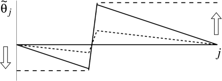
Figure 1: Different configurations of the reduced phase (16) that solve the static equations of motion (10) at the interior points. The ground state is $\tilde{\theta}_{j}\equiv 0$; it solves also the static equations (11)–(12) at the ends. Short dashes represent the saddle point (critical droplet) that sits at the top of the potential barrier responsible for metastability of the ground state. The solid polyline is a state on the other side of the barrier; it is referred to as a state with a $2\pi$ jump. Thermal decay corresponds to a transition through a vicinity of the critical droplet, and tunneling at low currents to transition from the ground state to the state with a $2\pi$ jump. (For tunneling at a high current, the final state needs to be found by the method described in Sec. V.) The state with a $2\pi$ jump does not solve the static equations at the ends, and so will be subject to forces there. Those will induce its evolution, over a longer timescale, towards the state shown by the long dashes (the initial direction of the evolution is shown by the arrows).

For the analysis of linear stability of these various solutions, we will need the Hessian—the matrix of second derivatives of the potential energy (5). It is a symmetric tridiagonal matrix, which we prefer to write in units of $I_{c}$:

$$M_{jj^{\prime}}=I_{c}^{-1}\frac{\partial^{2}U}{\partial\theta_{j}\partial\theta_{j^{\prime}}}\,.$$ (18)

Consistent with the boundary conditions (14)–(15), we restrict variations of $\theta_{j}$ to be supported at the interior points only; thus, in (18), $j,j^{\prime}=1,\dots,N-1$. Then, the diagonal elements of the Hessian are

$$M_{jj}=\cos(\theta_{j+1}-\theta_{j})+\cos(\theta_{j}-\theta_{j-1})\,,$$ (19)

and the off-diagonal ones are

$$M_{j,j+1}=M_{j+1,j}=-\cos(\theta_{j+1}-\theta_{j})\,.$$ (20)

We now consider the different types of solutions in turn.

III.1 Ground states

The simplest solution to (10) is the one where all the phase differences are equal, i.e., $\theta_{j}$ grows linearly with $j$ with some slope $\vartheta_{gs}$:

$$\theta_{j}=\vartheta_{gs}j\,.$$ (21)

This solves also the boundary equations (11)–(12) provided the slope satisfies

$$\sin\vartheta_{gs}=\bm{i}_{b}\,.$$ (22)

As already done previously, for $\bm{i}_{b}<1$, we take $\vartheta_{gs}$ to be the smaller root of (22) on $[0,\pi]$. Eq. (21) would remain a solution if we were to replace $\vartheta_{gs}$ with the larger root, $\pi-\vartheta_{gs}$. As we will see, however, that latter solution is linearly unstable.

We refer to (21) as the ground state (corresponding to a given $\bm{i}_{b}$). As noted earlier, the ground state is at best metastable (i.e., cannot be absolutely stable) for any $\vartheta_{gs}>0$. In terms of the reduced phase (16), the ground state becomes simply

$$\tilde{\theta}_{j}\equiv 0\,.$$

Thus, in general, we can think of the reduced phase as measuring fluctuations relative to the ground state.

Turning to analysis of linear stability, we note that all the cosines in the expressions (19)–(20) are now equal to $\cos\vartheta_{gs}$. The eigenvectors of the Hessian are then readily found: they are

$$\alpha_{j}^{(p)}=\sin(pj)\,,$$

where $p$ is a positive integer multiple of $\pi/N$. The corresponding eigenvalues are

$$\lambda_{p}=2(1-\cos p)\cos\vartheta_{gs}\,.$$ (23)

We see that the ground-state is linearly stable for $0\leq\vartheta_{gs}<\pi/2$. The solution, obtained by replacing $\vartheta_{gs}$ with the larger root of (22), i.e., $\pi-\vartheta_{gs}$, is linearly unstable. For the critical $\vartheta_{gs}=\pi/2$, the Hessian vanishes, and stability is determined by the leading non-linear term. That is cubic, and so the critical solution is unstable.

III.2 $2\pi$ jumps

The equality of the sines in (10) does not require equality of the arguments, and indeed (10) has solutions for which the phase differences across the links are not all equal. The simplest case is when they are all equal except for one, which differs from the rest by $2\pi$. For the phase itself, we then have two segments of linear growth joined together by a jump of approximately $2\pi$ (cf. Fig. 1). In terms of the reduced phase (16), the solution satisfying the boundary conditions (17) is

$$\tilde{\theta}_{j} = -\frac{2\pi j}{N}\,,\hskip 50.00008ptj=0,\dots,k\,,$$

$$\tilde{\theta}_{j} = -\frac{2\pi j}{N}+2\pi\,,\hskip 30.00005ptj=k+1,\dots,N\,.$$ (24)

The jump occurs on the link from $j=k$ to $j=k+1$, where $k$ can be any integer from 0 to $N-1$. We refer to it as a “$2\pi$ jump” even though the actual difference

$$\tilde{\theta}_{k+1}-\tilde{\theta}_{k}=2\pi(1-1/N)$$

is somewhat smaller than $2\pi$.

Analysis of linear stability is completely parallel to that for the ground state, with stability now determined by the sign of $\cos(\vartheta_{gs}-2\pi/N)$. For

$$N>4\,,$$ (25)

the solution is linearly stable for all $0\leq\vartheta_{gs}<\pi/2$. Smaller values of $N$ constitute special cases. For $N=2$, the solution is unstable for any of the above $\vartheta_{gs}$. For $N=3$, it is unstable for $\vartheta_{gs}<\pi/6$, while for $N=4$ it is stable as long as $\vartheta_{gs}\neq 0$ with the Hessian vanishing at $\vartheta_{gs}=0$. In what follows, we do not pursue detailed analysis of these special cases but simply assume that the condition (25) is satisfied.

What is the relevance of these solutions to decay of supercurrent? Our numerical results (a sample of which will be presented later) indicate that at temperatures $T\to 0$ and low currents, the state with a $2\pi$ jump is the final state of the tunneling process, by which the system, originally in a vicinity of the ground state, escapes through the potential barrier. The evolution after tunneling (the second stage in our two-stage description) proceeds in real time, according to the equations of motion (7) and (8)–(9) with $\tilde{\theta}_{j}$ = (24) and $\partial_{t}\tilde{\theta}_{j}\equiv 0$ as the initial conditions. Note that (24) solves the static equations at the interior points but not at the ends. Thus, the initial direction of the evolution is determined by the net forces in the boundary equations (8)–(9). The force at $j=0$ is equal to $I-I_{b}$, where

$$I=I_{c}\sin(\vartheta_{gs}-2\pi/N)$$

is the current on the solution, and $I_{b}=I_{c}\sin\vartheta_{gs}$ is the biasing current; the force at $j=N$ is $I_{b}-I$. For $N>4$ and $0\leq\vartheta_{gs}<\pi/2$, the difference $I-I_{b}$ is negative. This means that the initial direction of the real-time evolution is as indicated by arrows in Fig. 1, that is the system evolves towards the state shown in Fig. 1 by the long dashes.

The state shown by the long dashes has $\tilde{\theta}_{j}=c$ (a constant) for $j\leq k$ and $\tilde{\theta}_{j}=c+2\pi$ for $j\geq k+1$. Because each $\tilde{\theta}_{j}$ is defined modulo $2\pi$, this state differs from the ground state $\tilde{\theta}_{j}\equiv 0$ essentially by a constant shift of the phase. The transition to it from $\tilde{\theta}_{j}\equiv 0$, however, is observable as it generates a voltage pulse in the external circuit and involves work done by an external battery. This transition constitutes a phase slip. The work done by the battery is given by the negative of the second, non-periodic term in the potential energy (5). For instance, for the case shown in Fig. 1, it equals $2\pi I_{b}$.

We wish to reiterate that this special role of (24) as the final state of tunneling is characteristic of the low-current regime. At large currents, the final states need to be found by the method described in Sec. V.

III.3 Saddle points (critical droplets)

One more way to solve the sine equation (10) is to let all $\theta_{j+1}-\theta_{j}$ except one be equal, as in the case of a $2\pi$ jump, but let that one be $\pi$ minus any other. That is, if

$$\theta_{j+1}-\theta_{j}=\vartheta_{gs}+\gamma$$ (26)

for $j\neq k$ (where $\gamma$ is an as yet undetermined constant), then

$$\theta_{k+1}-\theta_{k}=\pi-(\vartheta_{gs}+\gamma)\,.$$ (27)

In terms of the reduced phase (16), the solution corresponding to (26) and satisfying the boundary conditions (14)–(15) is

$$\tilde{\theta}_{j} = \gamma j\,,\hskip 50.00008ptj=0,\dots,k\,,$$

$$\tilde{\theta}_{j} = \gamma(j-N)\,,\hskip 20.00003ptj=k+1,\dots,N\,.$$ (28)

Eq. (27) then becomes an equation for the slope $\gamma$. It has a solution,

$$\gamma=-\frac{\pi-2\vartheta_{gs}}{N-2}$$ (29)

for any $N>2$. Note that $\gamma<0$ for any $0\leq\vartheta_{gs}<\pi/2$ and is zero for the critical $\vartheta_{gs}=\pi/2$. In the latter case, the solution coincides with the ground state.

Even though the solution exists for any $N>2$, we restrict our attention to cases when

$$\cos(\gamma+\vartheta_{gs})=\cos\frac{N\vartheta_{gs}-\pi}{N-2}>0\,,$$ (30)

because then the solution has a special interpretation, discussed below. This inequality is always satisfied for $\vartheta_{gs}<\pi/2$ and $N>4$, a condition we have already imposed.

We will refer to the link form $j=k$ to $k+1$ as the “core” of the solution, even though, as we will see shortly, the energy is by no means concentrated at the core: the difference in the slope from the ground state is essential and leads to a contribution distributed over the entire length of the wire.

The solution is shown in Fig. 1 by the short dashes. The way it appears there implies that the slope $|\gamma|$ is smaller than $2\pi/N$, the slope of the solution with a $2\pi$ jump. One can verify that the condition for that is precisely the same as the condition of linear stability of the latter solution, derived previously.

Given that, as far as the slopes go, the present solution lies between the ground state and the state with a $2\pi$ jump, one may expect that it is a saddle point that sits at the top of the potential barrier separating the two states. We will now see that it is in fact a critical droplet—a saddle point that has exactly one negative mode and mediates thermally activated decay of the ground state.

A negative mode is an eigenvector of the Hessian corresponding to a negative eigenvalue. The cosines in eqs. (19)–(20) now are

$$\cos(\theta_{j+1}-\theta_{j})=\left\{\begin{array}[]{cc}\cos(\vartheta_{gs}+\gamma)\,,&j\neq k\,,\\ -\cos(\vartheta_{gs}+\gamma)\,,&j=k\,.\end{array}\right.$$

Thus, the eigenvalue problem for the Hessian is a discrete version of one-dimensional quantum mechanics with a localized potential. A negative mode corresponds to a bound state. The corresponding eigenvalue is of the form

$$\lambda_{-}=-\Lambda\cos(\vartheta_{gs}+\gamma)\,,$$ (31)

where $\Lambda>0$ depends only on $N$ and $k$.

For given $N$ and $k$, it is straightforward to find eigenvalues of the Hessian by numerical diagonalization. We have done that for a few small values of $N$, to convince ourselves that there is a unique negative mode in those cases. For $N\gg 1$, it is possible to prove existence and uniqueness of a negative mode without resorting to numerics.

As a sample of these results, consider the case when $N$ is odd and $k=\frac{1}{2}(N-1)$, meaning that the core of the solution is directly in the middle of the wire. We find, for instance, $\Lambda=1.303$ for $N=5$ and $\Lambda=1.330$ for $N=7$. The latter value is already close to the asymptotic

$$\Lambda=\frac{4}{3}$$ (32)

which corresponds to $N\to\infty$ and can be found analytically. The eigenvector corresponding to the negative mode is

$$\alpha^{(-)}_{j}=\left\{\begin{array}[]{cc}A\sinh(pj)\,,&j\leq\frac{1}{2}(N-1)\,,\\ -A\sinh[p(N-j)]\,,&j\geq\frac{1}{2}(N+1)\,.\end{array}\right.$$ (33)

where $A$ is a normalization coefficient, and $p$ is related to the eigenvalue by

$$\Lambda=2\cosh p-2\,.$$

For $N\to\infty$, $p=\ln 3$. Moving the core away from the middle causes $\Lambda$ to decrease, but the negative mode persists for all $k$, even $k=0$. In the latter case, the asymptotic value of at $N\to\infty$ is $p=\ln 2$, that is $\Lambda=\frac{1}{2}$.

Note that, unlike the droplet itself, which has linear “tails” extending to the ends of the wire (cf. Fig. 1), the negative mode is tightly localized: for instance, $p=\ln 3$ (in the $N\to\infty$ case) means that the magnitude of (33) decreases by a factor of 3 per link as one moves away from the core. As a consequence, the asymptotic result (32), obtained for a droplet in the middle of a long wire, has exponential accuracy in $N$ and will hold well even for droplets away from the middle, except for very short wires or droplets very near the ends.

When the droplet is strictly in the middle, the negative mode is antisymmetric about the core. This will hold approximately also away from the middle, except when the droplet is close to one of the ends. This antisymmetry has a simple interpretation: as clear from Fig. 1, adding an antisymmetric $\alpha^{(-)}_{j}$ with a small coefficient (i.e., moving along the negative mode) will deform the droplet either towards the ground state or towards the state with a $2\pi$ jump, precisely as expected of motion across the top of the potential barrier separating the two states.

III.4 Activation barrier

The energy of the critical droplet is obtained by substituting (26) and (27) into (5). In units of $I_{c}$, it equals

$${\cal E}_{drop}\equiv E_{drop}/I_{c}=-(N-2)\cos(\gamma+\vartheta_{gs})-\bm{i}_{b}(\theta_{N}-\theta_{0})\,.$$ (34)

This should be compared to the energy of the ground state,

$${\cal E}_{gs}\equiv E_{gs}/I_{c}=-N\cos\vartheta_{gs}-\bm{i}_{b}(\theta_{N}-\theta_{0})\,.$$ (35)

The difference between the two is the activation barrier for thermally activated phase slips (TAPS). Using (30), we obtain

$${\cal E}_{drop}-{\cal E}_{gs}=N\cos\vartheta_{gs}-(N-2)\cos\frac{N\vartheta_{gs}-\pi}{N-2}\,.$$ (36)

A curious property of (36) is that it is independent of $k$, the location of the droplet core. In a continuum model, that would imply existence of a zero mode—a zero eigenvalue of the Hessian—associated with the translational symmetry. In the present case, there is no such mode, as the symmetry with respect to infinitesimal translations is broken by the lattice.

Another convenient expression for the activation energy is obtained by using, instead of $\vartheta_{gs}$, the parameter $\epsilon$ defined by

$$\vartheta_{gs}=\frac{\pi}{2}-\epsilon\,.$$ (37)

Then,

$${\cal E}_{drop}-{\cal E}_{gs}=N\sin\epsilon-(N-2)\sin\frac{N\epsilon}{N-2}\,.$$ (38)

Eq. (36) has two interesting limits. The first is $N\gg 1$ with $\vartheta_{gs}$ fixed. In this case,

$${\cal E}_{drop}-{\cal E}_{gs}=2\cos\vartheta_{gs}-(\pi-2\vartheta_{gs})\sin\vartheta_{gs}+O(1/N)\,.$$ (39)

We see that the activation barrier remains finite in the limit of large length. That does not mean, however, that the energy difference (39) is accumulated locally, around the core of the droplet: the reduction (by the amount $|\gamma|$) of the slope of the droplet’s “tails” relative to the ground state, cf. (26), is essential and leads to a contribution distributed over the entire length of the wire.

Expressing $\vartheta_{gs}$ through the biasing current via (22), we find that, in the limit $N\to\infty$, the activation barrier (39) coincides exactly with that of a Josephson junction whose potential energy, as a function of the phase difference, is

$$U(\phi)=-I_{c}\cos\phi-I_{b}\phi\,.$$ (40)

As we show in the Appendix, this agreement is not limited to sinusoidal currents but extends to a much broader class of current-phase relations. It may not be obvious a priori, given especially that, in the wire, the activation process does not involve any changes of the phase difference between the ends, so in the computation of the activation barrier the last terms in (34) and (35) simply cancel each other. In contrast, in the junction (where the ground state is $\phi_{gs}=\arcsin\bm{i}_{b}$, and the critical droplet is $\phi_{drop}=\pi-\phi_{gs}$), the contribution of the last term in (40) is essential. Nevertheless, in the $N\to\infty$ limit, the agreement between the two cases is not entirely unexpected: it can be seen as an instance of the “theorem of small increments” LL:Stat , as already noted by McCumber McCumber in the context of the continuous GL theory.

The second interesting limit of (36) is $\vartheta_{gs}\to\pi/2$ with $N$ fixed, which corresponds to currents close to the critical. In this case, it is convenient to use the form (38) of the activation energy: the parameter $\epsilon$ is now small, and we can expand (38) in it. We obtain

$${\cal E}_{drop}-{\cal E}_{gs}=\frac{2N(N-1)\epsilon^{3}}{3(N-2)^{2}}+O(\epsilon^{5})\,.$$ (41)

In terms of the biasing current,

$$\epsilon=\sqrt{2}(1-\bm{i}_{b})^{1/2}+O[(1-\bm{i}_{b})^{3/2}]\,.$$ (42)

We see that the activation barrier is higher for smaller $N$, as might be expected, but the scaling at $\bm{i}_{b}\to 1$ is always the same $(1-\bm{i}_{b})^{3/2}$. This is the first of the results we have highlighted in the Introduction.

Finally, we note that, for $N>4$, there is also a double droplet, a state where eq. (27) (with a different value of $\gamma$) is used on two links. Its energy, in the same notation as in (38), is

$${\cal E}_{double}-{\cal E}_{gs}=N\sin\epsilon-(N-4)\sin\frac{N\epsilon}{N-4}$$ (43)

and is always larger than the energy of the single droplet.

IV Euclidean solutions and the crossover temperature

There can be no thermal activation at $T=0$, only quantum tunneling, so as the temperature is lowered past some point one mechanism of phase slips must give precedence to the other. In the semiclassical approximation, tunneling is described by classical solutions (instantons) that depend nontrivially on the Euclidean time $\tau=it$ and are periodic in $\tau$ with period $\beta=1/T$. Following periodic , we consider “periodic instantons”—solutions with two turning points (those are configurations where all the canonical momenta vanish simultaneously), one at $\tau=0$, and the other at half the period, $\tau=\frac{1}{2}\beta$. In the present case, the turning-point conditions are

$$\partial_{\tau}\tilde{\theta}_{j}(0)=\partial_{\tau}\tilde{\theta}_{j}(\beta/2)=0\,.$$ (44)

As discussed in periodic , a periodic instanton is expected to saturate the microcanonical tunneling rate $\Gamma_{micro}$, i.e., to give the most probable tunneling path at a fixed energy $E$; the period of the instanton in that case is determined by the energy. The same instanton will then saturate also the canonical (fixed temperature) tunneling rate

$$\Gamma_{can}(\beta)\sim\int dEe^{-\beta E}\Gamma_{micro}(E)\,,$$ (45)

provided the integrand here is peaked about the corresponding energy. As we discuss in more detail below, such is indeed the case in our present model.

The turning-point conditions (44), together with the spatial boundary conditions (17), define a boundary problem for the rectangle $0<j<N$, $0\leq\tau\leq\frac{1}{2}\beta$. The solution for $\frac{1}{2}\beta<\tau\leq\beta$ is obtained via

$$\tilde{\theta}_{j}(\tau)=\tilde{\theta}_{j}(\beta-\tau)\,.$$

The turning points $\tilde{\theta}_{j}(0)$ and $\tilde{\theta}_{j}(\beta/2)$ correspond, respectively, to the initial and final states of tunneling, that is, the states in which the system enters and leaves the classically forbidden region of the configuration space. The subsequent real-time evolution (the second stage in our two-stage description) proceeds with $\tilde{\theta}_{j}(\beta/2)$ as the initial state. Thus, $\tilde{\theta}_{j}(\beta/2)$ must be real. Since, for $0<j<N$, the Euclidean equations of motion contain no complex coefficients, the entire $\tilde{\theta}_{j}(\tau)$ must then be real, so we concentrate on real-valued solutions in what follows.

As shown in periodic , the main, exponential factor in the microcanonical tunneling rate is determined by the instanton’s “abbreviated” (Maupertuis) action per period, $\widetilde{S}(E)$, as follows:

$$\Gamma_{micro}(E)\sim e^{-\widetilde{S}(E)}\,.$$ (46)

So, the conditions for the integrand in (45) to have a maximum at $E$ are

$$-d\widetilde{S}/dE = \beta\,,$$ (47)

$$d^{2}\widetilde{S}/dE^{2} > 0\,.$$ (48)

If these are satisfied,

$$\Gamma_{can}(\beta)\sim e^{-S_{inst}(\beta)}\,,$$ (49)

where

$$S_{inst}(\beta)=\beta E+\widetilde{S}(E)\,.$$ (50)

Note that the normalization of (45) assumes that the ground state energy is zero; thus, $E$ in (50) is the energy of either turning point (by the Euclidean energy conservation, their energies are equal) relative to the ground state. Also, it is understood that $E$ is expressed through $\beta$ by means of (47). One result of that is the relation periodic

$$dS_{inst}/d\beta=E\,.$$ (51)

By a standard theorem of mechanics LL:Mech (translated to the Euclidean time), the right-hand side of (47) is the period of the solution, so (47) tells us that the period is the same as $\beta$. This is not unexpected but does go to show formally that (50) is the full (non-“abbreviated”) action of the instanton, relative to that of the ground state. Note that the exponential factor (49) accounts both for the suppression of the rate due to the tunneling per se (as represented by $\widetilde{S}$) and for that caused by the need to populate an initial state of energy $E$.

The inequality (48) is less trivial, in the sense that it may or may not be satisfied in a given system for a given range of energies. At small $E$, if the zero-energy instanton is known, one can construct an approximate periodic instanton by alternating instantons and anti-instantons in the $\tau$ direction periodic and check the condition (48) for it. For larger $E$, however, one typically has to resort to numerical studies. For the latter, the condition (48) can be somewhat more conveniently rewritten as

$$\frac{d^{2}S_{inst}}{d\beta^{2}}<0\,.$$ (52)

(By virtue of the relation between $E$ and $\beta$, the left-hand side here is the negative of $(d^{2}\widetilde{S}/dE^{2})^{-1}$.) Cases of varying complexity in the behavior of $S_{inst}(\beta)$ have been described in the literature (as briefly surveyed below), and we now discuss the specifics of the present case.

In general, the critical droplet undergoes a bifurcation at some $\beta=\beta_{bif}$, where it develops, in addition to its single $\tau$-independent negative mode, another, $\tau$-dependent one. The key distinction between different cases is in where that new negative mode leads at $\beta$ just above $\beta_{bif}$: it can lead to a limit cycle (a periodic instanton) in a vicinity of the critical droplet or, alternatively, to an entirely different region of the configuration space. This distinction is analogous to the one between the supercritical and subcritical forms of the usual Hopf bifurcation. For the case at hand, we find (numerically) that the former case (a nearby limit cycle) is realized. In addition, we find that a real-valued periodic instanton exists only for $\beta>\beta_{bif}$, and for all these $\beta$ the condition (52) is satisfied. In these respects, the present system is similar to the 2-dimensional Abelian Higgs model; the periodic instanton for that case was found numerically in Matveev . The behavior is different from that in the various versions of the 2-dimensional $O(3)$ sigma model or in the 4-dimensional SU(2) Yang-Mills-Higgs theory; numerical solutions for those cases were found, respectively, in Habib&al ; Kuznetsov&Tinyakov and Frost&Yaffe:1998 ; Frost&Yaffe:1999 ; Bonini&al .

At the bifurcation point, the condition (51) (recall that $E$ in it is measured from the ground state) implies

$$\frac{dS_{inst}}{d\beta}(\beta_{bif})=E_{drop}-E_{gs}\,.$$ (53)

The right-hand side here is the activation barrier of the preceding section. In other words, at this point, the $S_{inst}(\beta)$ curve touches the straight line

$$S_{drop}(\beta)=(E_{drop}-E_{gs})\beta\,,$$ (54)

corresponding to the thermal activation exponent. The condition (52) being satisfied for all $\beta>\beta_{bif}$ then implies that $S_{inst}$ deviates down from (54), so that, at least in the leading semiclassical approximation (where only the exponential factors count), tunneling has a larger rate than thermal activation. Thus, in the present case, $\beta_{bif}$ is the same as $\beta_{q}$, the point where one mechanism of phase slips overtakes the other. Note that the crossover temperature $T_{q}=1/\beta_{q}$ can be measured experimentally Li&al ; Aref&al ; Belkin&al .

Computation of $\beta_{bif}$ and so, in the present case, also of $T_{q}$ is standard. For the Lagrangian (4), the $\tau$-dependent normal modes are eigenfunctions of the operator

$$\hat{N}_{ij}=-C_{i}\delta_{ij}\partial_{\tau}^{2}+I_{c}M_{ij}\,,$$ (55)

where $i,j=1,\dots,N-1$, and $M_{ij}$ is the Hessian (18). As already mentioned, in this paper, we set all the capacitances $C_{j}$ at the interior points equal, $C_{j}=C$. Then, the eigenfunctions of (55) are of the form

$$\psi_{j}^{(n)}(\tau)=\alpha_{j}\cos(2\pi Tn\tau)\,,$$

where $\alpha_{j}$ is an eigenvector of the Hessian, and $n\geq 0$ is an integer. The choice of the cosine, rather than sine, here respects the boundary conditions (44). In this way, for each eigenvalue $\lambda$ of the Hessian, the $\tau$-dependent problem generates an infinite sequence of eigenvalues:

$$\lambda\to\lambda+\left(\frac{2\pi Tn}{\omega_{c}}\right)^{2}\,,$$ (56)

where

$$\omega_{c}=(I_{c}/C)^{1/2}\to(2eI_{c}/C)^{1/2}\,.$$ (57)

In the last relation, the arrow signifies transition to the physical units via (6). For $\lambda>0$, (56) can never produce a negative eigenvalue. For $\lambda=\lambda_{-}<0$, there is always the original one, corresponding to $n=0$. Another one appears at

$$T<T_{q}=\frac{\omega_{c}|\lambda_{-}|^{1/2}}{2\pi}\,,$$ (58)

which determines the crossover temperature.

Recall that $\lambda_{-}$ depends not only on $N$ and the biasing current $\bm{i}_{b}$, which are the parameters of the system, but also on $k$, the location of the droplet along the wire. The meaning of $T_{q}$ is that of the highest temperature for which tunneling is the main mechanism of phase slips, so in (58) we choose the largest $|\lambda_{-}|$ we can get at given $N$ and $\bm{i}_{b}$. As we have seen in the preceding section, this corresponds to $k$ in the middle of the wire. With this choice, $\lambda_{-}$ is given by (31) where $\Lambda$ now depends only on $N$.

Because $T_{q}$ can be measured experimentally, (58) can be used to estimate $\omega_{c}$. Let us use for this estimate the asymptotic large-$N$ value $\Lambda=4/3$, which, as we have seen, becomes a good approximation already at modest $N$. Setting $N=11$ and the biasing current to 90% of the critical current results in $\omega_{c}=7.5~{}T_{q}$. Since $I_{c}$ is also measurable, we can use (57) to convert this estimate of $\omega_{c}$ into an estimate of $C$. For $I_{c}=10~{}\mu\mbox{A}$ and $T_{q}=0.9~{}\mbox{K}$ (corresponding to the values in the experiment of Belkin&al ), we obtain $C=3.9\times 10^{-14}~{}\mbox{F}$. Note that this is the capacitance of a single segment of length $\Delta x$, not of the entire wire. We attribute this relatively large value of $C$ to the wire being in close proximity to large conductors (e.g., the center conductor strips Belkin&al ).

Next, consider the scaling of various quantities near the critical current. The Hessian matrix of the critical droplet is proportional to $\cos(\gamma+\vartheta_{gs})$. In view of (30), this means that all its eigenvalues, including $\lambda_{-}$, scale at $\bm{i}_{b}\to 1$ as the first power of $\epsilon=\pi/2-\vartheta_{gs}$, i.e., as $(1-\bm{i}_{b})^{1/2}$. Then, according to (58), $T_{q}$ scales as $(1-\bm{i}_{b})^{1/4}$. This implies that the system stays classical longer (i.e., until a lower temperature) as the current gets closer to the critical. The power-$1/4$ dependence, though, is quite weak, and it is not clear if this effect can be observed experimentally.

The Hessian of the ground state is proportional to $\cos\vartheta_{gs}=\sin\epsilon$ and so also scales as $\epsilon$. Thus, at $T\ll T_{q}$ the characteristic frequencies of Euclidean motion near the ground state and near the top of the barrier are both of order $\omega_{0}\sim\omega_{c}\sqrt{\epsilon}$. This suggests that, at these $T$, we can estimate the instanton action $S_{inst}$ by taking the product of the characteristic barrier height, $I_{c}(E_{sph}-E_{gs})$, and the common timescale $2\pi/\omega_{0}$. The result is

$$S_{inst}\sim 2\pi(I_{c}C)^{1/2}(1-\bm{i}_{b})^{5/4}\,.$$ (59)

We will see that the power-$5/4$ scaling law for $S_{inst}$ is well borne out numerically. Note that, due to the “critical slowing down” of the Euclidean dynamics at $\bm{i}_{b}\to 1$, this scaling law is different from the one for the barrier height itself. This is the second of the results highlighted in the introduction.

V Computation of the tunneling exponent

We now turn to a systematic study of periodic instantons in our system. The Euclidean equations of motion at the interior points, with all $C_{j}$ set equal to $C$, read

$$\partial_{\tau}^{2}\tilde{\theta}_{j}+\omega_{c}^{2}\left[\sin(\tilde{\theta}_{j+1}-\tilde{\theta}_{j}+\vartheta_{gs})-\sin(\tilde{\theta}_{j}-\tilde{\theta}_{j-1}+\vartheta_{gs})\right]=0\,,$$ (60)

where $\omega_{c}$ is the frequency (57). Recall that these are to be solved on the rectangle $0<j<N$, $0\leq\tau\leq\frac{1}{2}\beta$ with the boundary conditions (17) and (44). Note that this boundary problem depends only on the following dimensionless parameters: $N$, $\vartheta_{gs}$, and $\omega_{c}\beta$.

The Euclidean action corresponding to this boundary problem is

$$S_{E}=\int_{0}^{\beta}\!\!d\tau\left[\frac{C}{2}\sum_{j=1}^{N-1}(\partial_{\tau}\tilde{\theta}_{j})^{2}-I_{c}\sum_{j=0}^{N-1}\cos(\tilde{\theta}_{j+1}-\tilde{\theta}_{j}+\vartheta_{gs})\right].$$ (61)

The difference between (61) computed for the instanton and that for the ground state $\tilde{\theta}_{j}\equiv 0$ gives the instanton action $S_{inst}$ of the preceding section:

$$S_{inst}=S_{E}+\beta NI_{c}\cos\vartheta_{gs}\,.$$ (62)

Under the conditions stated there, $S_{inst}$ determines the exponential factor in the tunneling rate at temperature $T=1/\beta$, cf. eq. (49).

In the preceding, we concentrated on the dependence of $S_{inst}$ on the inverse temperature $\beta$. More generally, after extracting an overall factor, we can write is as a function of the three dimensionless parameters mentioned earlier and, in addition, of the instanton’s spatial location; the latter is labeled, as in the case of the critical droplet, by an integer $k$:

$$S_{inst}=(I_{c}C)^{1/2}\sigma_{inst}(N,\vartheta_{gs},\omega_{c}\beta;k)\,.$$ (63)

The function $\sigma_{inst}$ will be referred to as the reduced action. In what follows, we present results for it for the case when the instanton is in the middle of the wire; for odd $N$, this corresponds to $k=\frac{1}{2}(N-1)$. We have also found solutions, albeit with larger actions, with cores away from the middle.

Note that the activation exponent (54) can be written, similarly to (63), as

$$S_{drop}=(I_{c}C)^{1/2}\sigma_{drop}(N,\vartheta_{gs},\omega_{c}\beta)\,,$$

where

$$\sigma_{drop}(N,\vartheta_{gs},\omega_{c}\beta)=({\cal E}_{drop}-{\cal E}_{gs})\omega_{c}\beta$$ (64)

and, as in Sec. III, ${\cal E}$ denotes an energy measured in units of $I_{c}$. Thus, a comparison of $S_{inst}$ to $S_{drop}$ amounts to a comparison of $\sigma_{inst}$ to $\sigma_{drop}$.

For numerical work, we discretize eq. (60) on a uniform grid in the $\tau$ direction and solve the resulting difference equation by the Newton-Raphson method. This is the same general approach as used, for instance, in Frost&Yaffe:1999 ; Bonini&al to find periodic instantons in the Yang-Mills-Higgs theory.

V.1 Tunneling at low currents

We take up the case of high biasing currents in the next subsection. Here, we briefly discuss the case

$$\vartheta_{gs}\leq\pi/N\,,$$ (65)

which we refer to as low currents.

The condition (65) is a result of comparing the energy (35) of the ground state to the energy of the state with a $2\pi$ jump, eq. (24). When (65) is satisfied,

$$E_{jump}-E_{gs}=N[\cos\vartheta_{gs}-\cos(\vartheta_{gs}-2\pi/N)]>0\,.$$ (66)

The linear stability analysis in subsec. III.2 and the discussion there of the real-time evolution of the state with a $2\pi$ jump suggest that, for $N>4$, this state is the lowest-energy state in which the system can emerge after tunneling through the potential barrier. We have not rigorously proven this assertion, but it is consistent with the numerical results, and in this subsection we will proceed on the premise that it is correct. Then, (66) implies that, at low currents, a phase slip requires tunneling “up” in energy or, more precisely, that the initial state of tunneling cannot be the ground state but must be thermally activated. This means that (at low currents) the instanton action $S_{inst}$ retains a nontrivial dependence on $\beta$ for arbitrarily large $\beta$ (i.e., low temperatures), namely, that in this limit

$$S_{inst}(\beta)\approx(E_{jump}-E_{gs})\beta\,.$$ (67)

The slope here, given by (66), is not as large as the full barrier height, eq. (36), because the system does not need to activate to the top of the barrier but only to an initial state with enough energy to tunnel to the state with a $2\pi$ jump. This activated behavior can be traced back to the boundary conditions (17) the phase must satisfy during tunneling and so is ultimately an effect of the bulk superconducting leads. As such, it was identified in a different (continuum) model of the wire in Khlebnikov:CG .

An example of numerically found low-current periodic instanton is shown in Fig. 2. The front of the plot ($\tau=0$) corresponds to the initial state of tunneling, and the back ($\tau=\frac{1}{2}\beta$) to the final state. The difference between the initial state and the ground state $\tilde{\theta}_{j}\equiv 0$ represents the thermal excitation required by the argument above. The final state coincides, as far as we can tell, with the state with a $2\pi$ jump.

Figure 2: A low-current periodic instanton. The plot shows the reduced phase $\tilde{\theta}_{j}(\tau)$, which is equal to the difference between the original phase variable $\theta_{j}(\tau)$ and the ground state $\theta_{j}=\vartheta_{gs}j$. The values of the parameters are $N=11$, $\vartheta_{gs}=0.2$, $\omega_{c}\beta=20$, and $k=5$. Recall that $\sin\vartheta_{gs}$ is the biasing current in units of the critical. Only the interior points $j=1,\dots,10$ and half of the period $[0,\frac{1}{2}\beta]$ in the $\tau$ direction are shown; $\tau$ is in units of $\omega_{c}^{-1}$.

V.2 Tunneling at arbitrary currents

A sample result for $\tilde{\theta}_{j}(\tau)$ for a comparatively large current, is shown in Fig. 3. The key distinction between this instanton and the one for small current, Fig. 2, is that now the system tunnels practically from the ground state. That is so, even though the temperature for this plot is only about a factor of 3 smaller than the crossover $T_{q}$. In the final state, the phase still has a characteristic jump at the tunneling location, but the magnitude of the jump is reduced compared to the low-current case.

Figure 3: A high-current periodic instanton. The reduced phase $\tilde{\theta}_{j}(\tau)$ for the instanton with the same $N$, $\omega_{c}\beta$, and $k$ as in Fig. 2, but with a larger $\vartheta_{gs}=1$.

In Fig. 4, we plot the reduced action $\sigma_{inst}$, as defined by (63), as a function of the half-period for several values of $\vartheta_{gs}$. These plots illustrate the crossover from the high-temperature (small $\beta$) regime, where the main mechanism of phase slips is thermal activation, to the low-temperature (large $\beta$) regime, where the main mechanism is tunneling. We see that, after the instanton first appears at $\beta=\beta_{q}$, its action for all $\beta>\beta_{q}$ lies below the straight line representing thermal activation—the behavior announced in Sec. IV. The crossover temperatures for all the curves shown are fairly close to one another and correspond to $\frac{1}{2}\omega_{c}\beta_{q}\approx 3$. For lower values of the current, the crossover leads to a transition from the high-temperature activated behavior to one with a smaller slope, as anticipated in subsec. V.1 (and found for a continuum model in Khlebnikov:CG ). For larger currents, the action quickly saturates at the zero-temperature value.

Figure 4: Solid lines: the reduced instanton actions $\sigma_{inst}$ for $N=11$, $k=5$ (instanton in the middle of the wire), and several values of $\vartheta_{gs}$. These are plotted as functions of the half-period $\frac{1}{2}\beta$, where $\beta$ is units of $\omega_{c}^{-1}$. The values of $\vartheta_{gs}$ increase in increments of 0.1 from top to bottom. Dashed lines: the straight lines (64) representing the over-barrier activation exponents for the same $\vartheta_{gs}$. The three smaller values of $\vartheta_{gs}$ correspond to the low-current regime (cf. subsec. V.1), where the instanton action displays the activated (linear) behavior (67) at large $\beta$ (though with a slope reduced compared to the full barrier height).

Next, consider dependence of the results on $N$, the length of the wire. The low-current condition (65) is obviously sensitive to $N$. The results at higher currents, however, are not particularly so. For instance, for $\vartheta_{gs}\geq 1$, doubling the length from $N=11$ to $N=21$ makes the actions smaller by only a few percent.

Finally, let us discuss the case of currents close to the critical, $\vartheta_{gs}\to\pi/2$. In this regime, we are mostly interested in the scaling law obeyed by the asymptotic value of $\sigma_{inst}$ at $\beta\to\infty$, as a function of $\epsilon=\pi/2-\vartheta_{gs}$. We find that the power-$5/4$ scaling anticipated in (59) is well borne out. Numerically, for $N=11$,

$$\sigma_{inst}(\beta\to\infty)=5.5~{}\epsilon^{5/2}$$ (68)

at $\epsilon\to 0$; for $N=21$, the coefficient changes from 5.5 to 5.2. Substituting (42) for $\epsilon$, we find that (68) corresponds to

$$S_{inst}(T\to 0)\approx 13\left(\frac{\hbar I_{c}C}{8e^{3}}\right)^{1/2}(1-\bm{i}_{b})^{5/4}\,,$$ (69)

where we have also used (6) to convert $(I_{c}C)^{1/2}$ to the physical units. For $I_{c}=10~{}\mu{\mbox{A}}$ and $C=3.9\times 10^{-14}~{}\mbox{F}$ (the estimate obtained at the end of Sec. III), eq. (69) gives $S_{inst}\approx 460(1-\bm{i}_{b})^{5/4}$. This estimate suggests that, even for this large value of $C$, raising the current to within 10% of the critical will make the rate large enough for quantum phase slips to become observable.

VI Discussion

In this paper, we have looked at both classical and quantum mechanisms of decay of supercurrent in superconducting nanowires. These mechanisms correspond, respectively, to over-barrier activation and tunneling. For the former, our main conclusion is that the power-3/2 scaling law (1) for the activation barrier, often observed experimentally, is readily reproduced in a discrete model of the wire. That is so even though we assume that the values of the phase at the ends remain unchanged during the activation process (a boundary condition attributed to the presence of bulk superconducting leads) and keep $N$, the length of the wire, finite and possibly small when sending the current to the critical.

Next, we have found that, in this discrete model, the crossover to the quantum regime occurs in a continuous manner similar to a supercritical Hopf bifurcation. We have found numerically the Euclidean solutions (periodic instantons) that describe tunneling for temperatures ranging from $T$ just below the crossover $T_{q}$ to $T$ close to zero. We have also observed that the slowing down of the Euclidean dynamics near the critical current, leads to the power-5/4 scaling law for the tunneling exponent at $T\ll T_{q}$.

Physically, the discrete model represents the idea that the spatial size of a phase slip is determined by the size of a Cooper pair (Pippard’s coherence length in the clean limit or its counterpart, discussed in Sec. II, in the dirty limit). Such a phase slip will appear point-like in any local theory that deals with the order parameter alone, for instance, in the standard GL theory. In other words, the activation path described here is physically distinct from that mediated by the LA saddle point LA of the GL model (and it is, then, perhaps not surprising that the activation barrier follows a different scaling law).

Finally, let us return to the question asked in the beginning of this paper, namely, whether it is possible to represent the results obtained so far as consequences of the dynamics of a single phase variable. We note at once that this variable cannot be the phase difference between the ends of the wire, because we assume that the phases at the ends do not change at all during either activation or tunneling. A variable that does look suitable is the jump, $\vartheta_{core}=\theta_{k+1}-\theta_{k}$, of the phase across the core of a phase slip. This variable is “emergent,” in the sense that it refers specifically to solutions describing phase slips: critical droplets and periodic instantons. In Sec. V, we have seen that, at large $N$ and low currents, $\vartheta_{core}$ changes during tunneling by nearly the full $2\pi$. On the other hand, it changes by only a small amount at currents near the critical. These properties are consistent with the intuition about how the right variable should behave. We expect that a phenomenological theory of $\vartheta_{core}$, based on a suitable effective potential, will be able to reproduce the various scaling laws discussed in the present paper.

The author thanks A. Bezryadin for comments on the manuscript.

Appendix A Activation barrier in the general case

Here, we generalize the results of Sec. III to the case when the current in each link is a periodic but non-sinusoidal function of the phase difference:

$$I_{j,j+1}=F^{\prime}(\theta_{j+1}-\theta_{j})\,.$$ (70)

We assume that $F^{\prime}(\vartheta)$ is the derivative of a smooth $2\pi$-periodic function $F(\vartheta)$ (the potential) and is subject only to the following two conditions. (i) $F^{\prime}(\vartheta)$ is odd (a consequence of time-reversal invariance). This implies $F^{\prime}(0)=0$ and, due to the periodicity, also $F^{\prime}(\pi)=0$. (ii) $F^{\prime}(\vartheta)$ has exactly one maximum (and no minima) on $(0,\pi)$. The maximum value of $F^{\prime}$ is the critical current $I_{c}>0$.

Condition (ii) implies that for any $0\leq I<I_{c}$, the equation $F^{\prime}(\vartheta)=I$ has exactly two roots on $[0,\pi]$. We will use the following notation: if one of the roots is $\vartheta_{1}$, we will write the other as

$$\vartheta_{2}=\vartheta_{1}^{\vee}$$ (71)

and refer to it as the coroot of $\vartheta_{1}$. As an example, for the sinusoidal $F^{\prime}$, $\vartheta^{\vee}=\pi-\vartheta$.

In the ground state corresponding to biasing current $I_{b}$, all the phase differences $\theta_{j+1}-\theta_{j}$ are equal to $\vartheta_{gs}$, the smaller root of $F^{\prime}(\vartheta_{gs})=I_{b}$. For the critical droplet, all of them except one are equal to $\vartheta_{gs}+\gamma$, and the remaining one to $(\vartheta_{gs}+\gamma)^{\vee}$. By our choice of the boundary conditions, the total phase difference $\theta_{N}-\theta_{0}$ for the droplet must be the same as for the ground state. This leads to the following equation for $\gamma$:

$$(N-1)\gamma+(\vartheta_{gs}+\gamma)^{\vee}=\vartheta_{gs}\,.$$ (72)

In the limit when $N\to\infty$ with $\vartheta_{gs}$ fixed, there is a unique solution:

$$\gamma=-\frac{1}{N}\left(\vartheta_{gs}^{\vee}-\vartheta_{gs}\right)+O(1/N^{2})\,.$$ (73)

We will assume that, even if $N$ is not particularly large, it remains large enough for the solution to exist and be unique. (For the sinusoidal $F^{\prime}$, this leads to the condition $N>2$ mentioned in the main text.)

The energy of the critical droplet, relative to the ground state, is

$$E_{sph}-E_{gs}=(N-1)F(\vartheta_{gs}+\gamma)+F[(\vartheta_{gs}+\gamma)^{\vee}]-NF(\vartheta_{gs})\,.$$ (74)

Special cases arise when $\gamma$ is small, and we can expand (74) in it. Expanding to the second order and using (72) and the definition of the coroot, we obtain

$$E_{sph}-E_{gs}=F(\vartheta_{gs}^{\vee})-F(\vartheta_{gs})+I_{b}(\vartheta_{gs}-\vartheta_{gs}^{\vee})+O(NF^{\prime\prime}\gamma^{2})\,.$$ (75)

The second derivative in the last term is taken at $\vartheta_{gs}$. At $N\gg 1$, $\gamma$ is $O(1/N)$, so in the limit $N\to\infty$ (75) coincides perfectly with the activation energy of a Josephson junction whose potential is $U(\phi)=F(\phi)-I_{b}\phi$.

Next, consider $I_{b}$ close to the critical current $I_{c}$ (with $N$ fixed). In this case, $\vartheta_{gs}^{\vee}-\vartheta_{gs}\equiv 2\epsilon$ is small, and $\gamma$ is of order $\epsilon$. Upon the expansion

$$F(\vartheta_{gs}^{\vee})-F(\vartheta_{gs})=I_{b}(\vartheta_{gs}^{\vee}-\vartheta_{gs})+O(\epsilon^{3})\,,$$ (76)

we see that the $O(\epsilon)$ terms in (75) cancel. The last term in (75) is $O(\epsilon^{3})$, because near the maximum of $F^{\prime}$ the second derivative $F^{\prime\prime}$ is small, here of order $\epsilon$. Since $\epsilon$ scales as $(1-I_{b}/I_{c})^{1/2}$, we obtain, for this general case, the same power-3/2 scaling (1) as found earlier for the sinusoidal $F^{\prime}$.

References

- (1) A. Belkin, M. Belkin, V. Vakaryuk, S. Khlebnikov, and A. Bezryadin, Phys. Rev. X 5, 021023 (2015).
- (2) P. Li, P. M. Wu, Y. Bomze, I. V. Borzenets, G. Finkelstein, and A. M. Chang, Phys. Rev. Lett. 107, 137004 (2011).
- (3) T. Aref, A. Levchenko, V. Vakaryuk, and A. Bezryadin, Phys. Rev. B 86, 024507 (2012); T. Aref, Ph.D. thesis, University of Illinois, 2010.
- (4) T. A. Fulton and L. N. Dunkleberger, Phys. Rev. B 9, 4760 (1974).
- (5) J. S. Langer and V. Ambegaokar, Phys. Rev. 164, 498 (1967).
- (6) M. Tinkham, J. U. Free, C. N. Lau, and N. Markovic, Phys. Rev. B 68, 134515 (2003).
- (7) K. A. Matveev, A. I. Larkin, and L. I. Glazman, Phys. Rev. Lett. 89, 096802 (2002).
- (8) L. D. Landau and E. M. Lifshitz, Statistical Physics, Part 1 (Butterworth-Heinemann, Oxford, 1980), Sec. 15.
- (9) D. E. McCumber, Phys. Rev. 172, 427 (1968).
- (10) S. Y. Khlebnikov, V. A. Rubakov, and P. G. Tinyakov, Nucl. Phys. B 367, 334 (1991).
- (11) R. M. Bradley and S. Doniach, Phys. Rev. B 30, 1138 (1984).
- (12) A. Bezryadin, Superconductivity in Nanowires: Fabrication and Quantum Transport (Wiley-VCH, Weinheim, 2013), Appendix A.
- (13) A. O. Caldeira and A. J. Leggett, Phys. Rev. Lett. 46, 211 (1981).
- (14) L. D. Landau and E. M. Lifshitz, Mechanics (Pergamon Press, Oxford, 1976), Sec. 49.
- (15) V. V. Matveev, Phys. Lett. B 304, 291 (1993) [hep-lat/9302006].
- (16) S. Habib, E. Mottola, and P. Tinyakov, Phys. Rev. D 54, 7774 (1996) [hep-ph/9608327].
- (17) A. N. Kuznetsov and P. G. Tinyakov, Phys. Lett. B 406, 76 (1997) [hep-ph/9704242].
- (18) K. L. Frost and L. G. Yaffe, Phys. Rev. D 59, 065013 (1999) [hep-ph/9807524].
- (19) K. L. Frost and L. G. Yaffe, Phys. Rev. D 60, 105021 (1999) [hep-ph/9905224].
- (20) G. F. Bonini, S. Habib, E. Mottola, C. Rebbi, R. L. Singleton, and P. G. Tinyakov, Phys. Lett. B 474, 113 (2000) [hep-ph/9905243].
- (21) S. Khlebnikov, Phys. Rev. B 77, 014505 (2008) [arXiv: 0709.1820 [cond-mat.supr-con]].