The effect of detector nonlinearity on WFIRST PSF profiles for weak gravitational lensing measurements

Abstract

Weak gravitational lensing (WL) is one of the most powerful techniques to learn about the dark sector of the universe. To extract the WL signal from astronomical observations, galaxy shapes must be measured and corrected for the point spread function (PSF) of the imaging system with extreme accuracy. Future WL missions—such as NASA’s Wide-Field Infrared Survey Telescope (WFIRST)—will use a family of hybrid near-infrared CMOS detectors (HAWAII-4RG) that are untested for accurate WL measurements. Like all image sensors, these devices are subject to conversion gain nonlinearities (voltage response to collected photo-charge) that bias the shape and size of bright objects such as reference stars that are used in PSF determination. We study this type of detector nonlinearity (NL) and show how to derive requirements on it from WFIRST PSF size and ellipticity requirements. We simulate the PSF optical profiles expected for WFIRST  and measure the fractional error in the PSF size ($\Delta R/R$) and the absolute error in the PSF ellipticity ($\Delta e$) as a function of star magnitude and the NL model. For our nominal NL model (a quadratic correction), we find that, uncalibrated, NL can induce an error of $\Delta R/R=1\times 10^{-2}$ and $\Delta e_{2}=1.75\times 10^{-3}$ in the H158 bandpass for the brightest unsaturated stars in WFIRST. In addition, our simulations show that to limit the bias of $\Delta R/R$ and $\Delta e$ in the H158 band to $\sim 10\%$ of the estimated WFIRST error budget, the quadratic NL model parameter $\beta$ must be calibrated to $\sim 1\%$ and $\sim 2.4\%$, respectively. We present a fitting formula that can be used to estimate WFIRST detector NL requirements once a true PSF error budget is established.

1 Introduction

Weak gravitational lensing (WL) has been identified as a powerful probe of the nature and evolution of the components of the Universe. In particular, cosmic shear—the subtle distortions of background galaxy shapes by the large-scale structure of the Universe—constrains the properties of dark matter and dark energy through the measurement of the expansion history and growth of structure of the Universe (Réfrégier, 2003; Hoekstra and Jain, 2008; Kilbinger, 2015). WL measurements also allow the testing of the validity of General Relativity that relates the gravitational potential to the matter-energy distribution. Several surveys in the visible part of the spectrum of $>1000$ deg² of the sky are currently underway and use the WL signal from hundreds of millions of galaxies as one of their central scientific techniques (e.g., the Dark Energy Survey (DES), Diehl and Dark Energy Survey Collaboration 2012, Jarvis et al. 2015; the Kilo-Degree Survey (KiDS), Kuijken et al. 2015; and the Hyper Suprime-Cam Survey (HSC), Miyazaki et al. 2012). In addition, future ground- and space-based surveys and missions in the visible and near infra-red (NIR) are planned to image more than O($10^{9}$) galaxies in the next decade (e.g., the Large Synoptic Survey Telescope (LSST), Ivezic et al. 2008; the Euclid spacecraft, Laureijs et al. 2011; and NASA’s Wide-Field Infrared Survey Telescope (WFIRST), Green et al. 2012, Spergel et al. 2013, Spergel et al. 2015).

The process of extracting the WL signal from images of the sky, in the presence of intrinsic galaxy ellipticity variations that are $\sim$ 0.4 r.m.s, is highly non-trivial. It must be done through a statistical analysis of large galaxy samples, with a careful control of systematic uncertainties. The dominant signal produced by WL can be described by a local linear transformation of the source image that produces a shear (a complex, spin-2 field of components $\gamma_{1}$ and $\gamma_{2}$) and a scalar magnification, both of which have an r.m.s. amplitude of only $\sim 2\%$ in the case of cosmic shear. Most of the background galaxies usable by WL are at hight redshift (with low signal-to-noise (S/N) ratio) and with a size comparable or smaller than the Point Spread Function (PSF) of the imaging system. Incorrect estimation of the size of the PSF induces a modulation in the signal (multiplicative errors), and errors in the estimation of the PSF ellipticity propagate into asymmetries that produce coherent spurious patterns (additive errors) that mimic the WL signal. Bright stars are commonly used to estimate the PSF, and then this information must be interpolated to the observed galaxy positions to deconvolve the PSF contribution and measure the galaxy shape (in the form of a complex ellipticity $e=e_{1}+ie_{2}$) to estimate the shear field. This interpolation step introduces systematic errors if the information inferred from the stars does not fully constrain the PSF at the galaxy position with the required accuracy. In order not to bias the determination of dark energy and other cosmological parameters in Stage IV surveys (in the language of Albrecht et al. 2006), the ellipticity and relative size of the PSF must be known to an accuracy of O(10^-3) (Huterer et al. 2006, Amara and Réfrégier 2008, Paulin-Henriksson et al. 2008, Paulin-Henriksson et al. 2009, Massey et al. 2013, Cropper et al. 2013) or better ($4.7\times 10^{-4}$ for the knowledge of the WFIRST PSF ellipticity, Spergel et al. 2013).

Systematic errors that originate from a telescope’s detectors (image sensors) introduce biases in astronomical observables such as photometry and astrometry that propagate into shear measurement biases. These type of errors have been extensively studied in the case of thick, fully-depleted, high-resistivity Charge Coupled-Devices (CCDs), which are the detectors of choice for many current and planned surveys such as DES, HSC, and LSST (e.g., Stubbs 2014, Plazas et al. 2014, Gruen et al. 2015), as well as in other types of CCDs (e.g., Prod’homme et al. 2014, Niemi et al. 2015). It is of great importance to quantify the impact of these sensor effects on the inference of cosmological parameters, in particular through WL (Jarvis 2014, Mandelbaum 2015, Meyers and Burchat 2014). Future missions such as the James Webb Space Telescope and WFIRST will utilize a family of near-infrared detectors that are also subject to effects such as nonlinearity, reciprocity failure (Bohlin et al. 2005, Biesiadzinski et al. 2011), interpixel capacitance (IPC; McCullough 2008, Kannawadi et al. 2015), and persistence (Smith et al. 2008). These effects can imprint biases on weak lensing shape measurements if not taken into account.

In this paper we study the effect of nonlinear detector conversion gain (voltage response to collected photo-charge) on PSF size and ellipticity in the context of the NIR detectors that will be used by NASA’s WFIRST mission. This type of detector nonlinearity (NL) will tend to attenuate the measured flux in bright stars, broadening the inferred PSF. In other words, NL preferentially depresses the flux in the core of the PSF relative to the wings, thus complicating its deconvolution from the observed galaxy image, which itself is fainter and less subject to the effects of NL. In addition, even though NL does not induce a spurious ellipticity by itself, it modifies the PSF ellipticity if the PSF is anisotropic. Our analysis is also useful to set preliminary requirements on NL for these sensors. Once characterized, NL can be corrected in each image, and remaining residuals will depend on the accuracy in the knowledge of the NL parameters and their spatial variation. We use the python/C++ code GalSim (Rowe et al., 2015) to simulate WFIRST PSF profiles and to analyze the impact of NL on PSF size and ellipticity.

In Section 2 we summarize the main characteristics of the NIR detectors that will be used in WFIRST  and describe NL. In Section 3 we describe the simulations we create to study NL for WFIRST PSF profiles. Section 4 presents our main results on fractional errors in size and absolute errors in ellipticity caused by NL, as function of relevant parameters such as the model parameters and PSF magnitude. We also study the effect of the spatial variability of the NL model across the pixel array. We conclude in Section 5 with a discussion of our results and how they can be used in the derivation of NIR detector specifications to satisfy WL accuracy requirements.

2 Voltage nonlinearity in the NIR detectors of WFIRST

The WFIRST mission will use a 2.4 m telescope equipped with a Wide Field Instrument (WFI) with 6 bandpass filters: Z087, Y106, J129, W149, H158, and F184 (Spergel et al. 2015). The WFI will perform a high-latitude survey (HLS), imaging over an area of 2200 deg² in four NIR ($\sim 0.92$–$2.00\ \mu$m) bands (Y106, J129, H158, and F184) down to a 5$\sigma$ point-source AB magnitude of 26.7 in the J129 band. The weak lensing program in the HLS will measure shapes of about 380 million galaxies in the J129, H158, and F184 bands (Spergel et al. 2015).

The WFI possesses a wide-field channel that has a Focal Plane Assembly (FPA) of 18 $4k\times 4k$ HgCdTe (mercury, cadmium, and telluride) NIR detectors, arranged in a $6\times 3$ layout and with a pixel size and scale of 10 $\mu$m and 0.11 arcseconds per pixel, respectively. The HgCdTe NIR detectors are manufactured by Teledyne Imaging Systems, and are part of a family of detectors known as Hawaii-XRG (HXRG), where X denotes the detector width in thousands of pixels.

The detector arrays are fabricated with a hybrid complementary metal-oxide-semiconductor (CMOS) architecture, which combines the qualities of HgCdTe to detect infra-red light (e.g., altering the relative molar contributions of mercury and cadmium allows one to tune the band gap by up to an order of magnitude) and the advanced readout performance of integrated circuits. Light is absorbed, converted to charge through the photoelectric effect, and collected by electric fields generated by a reverse-biased p-n junction in the detector layer. The charge per pixel is then converted to a voltage and amplified through a source follower. This operation is performed in the silicon readout integrated circuit (ROIC) layer, which is connected to the HgCdTe detection layer by indium interconnects (one indium bump per pixel). Finally, the ROIC transfers the signal (and for this it is also known as “multiplexer”) to the off-chip electronics at the edge of the FPA, where it is digitized through analog-to-digital converters (Beletic et al., 2008).

An ideal detector would produce a measurable signal that is proportional to the detected photons. However, there are several places in the signal chain where this expected linearity is not realized, and the conversion of charge to measured voltage (or digital numbers) becomes non-linear. Each pixel’s p-n junction acts as a parallel-plate capacitor, and as charge accumulates the depletion region narrows, causing a deviation from linearity of the charge-to-voltage conversion relation. Nonlinearity can also be introduced through the electronic gain of the ROIC. Furthermore, the charge accumulation rate might be a function of the photon-accumulation rate, an effect known as count-rate nonlinearity or reciprocity failure (RF) (Smith et al. 2008, Biesiadzinski et al. 2011). The first two types of nonlinearity depend only on fluence (integrated signal) as opposed to RF, which is flux dependent. They can be analyzed together in a single transfer function typically called “nonlinearity” (NL). We study the impacts of NL (more relevant at high signals) on PSF measurements in this paper, while we leave investigations on the consequences of RF (relevant at lower signals) on WL measurements for future work.

Assuming that the dominant contribution to nonlinearity is the varying capacitance of the pixel p-n junction, we find that the correction to the detector signal is well-approximated by a quadratic term:

$$S(Q)=Q-\beta Q^{2}$$ (1)

Here, $Q$ is the true number of elementary charges collected in the pixel, $S$ is the number inferred from the voltage change at the sense node, and $\beta$ is a constant. To estimate $\beta$, we compute $Q(V)=C(V)*V/q_{e}$, where $q_{e}$ is the elementary charge, and the total capacitance is given by the varying junction capacitance plus a constant $C(V)=C_{\rm jn}(V)+C_{\rm fix}$. The junction capacitance varies as (McCaughrean 1987)

$$C_{\rm jn}(V)\propto(1+V/V_{bi})^{-1/2}\;.$$ (2)

Here, $V_{bi}$ is the “built in” potential of the junction and $V=V_{\rm DSUB}-V_{\rm RESET}+\delta V$, where $V_{\rm DSUB}$ is the constant potential at the diode cathode, $V_{\rm RESET}$ is the initial potential at the anode, and $\delta V$ is the change in anode potential due to accumulated photocharge. As an example, we substitute measurements of a 2.4$\mu$m cutoff H2RG by Finger 2006:

$$V_{\rm bi} = 0.412\ {\mbox{V}}$$

$$V_{\rm DSUB} = 1\ {\mbox{V}}$$

$$V_{\rm RESET} = 0.5\ {\mbox{V}}$$

$$C_{\rm fix} = 17.8\ {\mbox{f}F}$$

$$C_{\rm jn}(V=.912\ {\mbox{V}}) = 30\ {\mbox{f}F}$$

Using these parameters to compute $Q(V)$ for $0\leq\delta V\leq 0.3$ V (corresponding to maximum $Q$=60115) and then inverting to find $S(Q)$, we find it is well-fit (to 0.1% or better) by Eq. 1 with $\beta=1.18\times 10^{-6}$. In practice, HXRG calibrations have included additional polynomial parameters which can reduce residuals, extend the range of valid $Q$, and account for additional nonlinear effects (Hilbert 2004, Hilbert 2008, Hilbert 2014); however, the additional parameters are highly degenerate, resulting in large variances in the fitted values. For our purposes, it suffices to analyze the shape-distorting effects of nonlinearity using a single parameter, $\beta$, which encapsulates most of the effect. In this paper we chose a nominal value of $\beta_{0}=5\times 10^{-7}$, which is near the midpoint of the measured range for $\beta$ in Hilbert 2014.

To illustrate the effect of NL on photometry, consider nearly saturated stars in the HLS. Using PSF profiles with a simulated AB magnitude up to 18.3 for an exposure time of 168.1 seconds (expected for the HLS), the total flux in each band is shown in Table 1, along with the peak pixel value. When the profile is drawn on a pixelated postage stamp with a scale of $p=0.11$ arcseconds and placed on the center of the pixel, this particular magnitude produces a peak charge of $\sim 1\times 10^{5}$ e^- (Y106 band, see Table 1), which represents about 90% of the typical pixel full well value of $1.1\times 10^{5}$ e^-. At this level of charge, the signal attenuation due to NL for the nominal $\beta_{0}$ value is about 5% (Eq. 1).

Calculations with the Trilegal galaxy model (Girardi et al., 2012) show that there will be approximately 20 stars at or brighter than this magnitude (18.3) and flux level per detector. We assume that galaxies will have about two orders of magnitude fewer total electrons than bright stars, and therefore for this quadratic model, star shapes are distorted by NL and galaxies are (approximately) not, which would result in an incorrect PSF correction if not accurately calibrated. Thus our goal is apply NL to simulated WFIRST PSF profiles and quantify the impact on PSF properties such as size and shape.

3 Methods

3.1 Simulations

We use the publicly available GalSim code (v1.3) to simulate the impact of NL on the WFIRST PSF shape and size. GalSim is a python/C++ open-source code that allows the user to create simulations of astronomical objects, and it was developed by the weak lensing community to investigate shape measurement algorithms and systematics.

Kannawadi et al. (2015) have developed within GalSim v1.3 a WFIRST module called “galsim.
wfirst”, which allows the simulation of a PSF profile according to the optical design characteristics of the WFIRST WFI (Pasquale et al., 2014)

For this work, we have created simulations in the four bands of the HLS. A central circular obscuration ($30\%$; linear in value) and six support struts are included as well.

The module generates PSF models that do not include pointing jitter nor charge diffusion. These effects could be added to the profile (e.g., by means of an extra convolution with a Gaussian profile in the case of diffusion), but we did not include them in our simulations. Their effect would be to create a slightly larger PSF, reducing the impact of NL. Their omission makes our results slightly conservative.

The ellipticity of the WFI PSF varies over the field of view due to optical aberrations. To make our results conservative, we simulate only detector #18, whose PSF was determined to have the largest ellipticity (see Section 3.2 for a description of the shape measurement method used) across all bands among all the detectors (Table 1). We also evaluate the PSF at the mean wavelength weighted by each bandpass or effective wavelength. We then form an effective PSF by convolving the profile with a 2D top-hat profile of length equal to the nominal angular scale of the WFIRST WFI ($0.11$ arcseconds per pixel).

Band	Min. $\lambda$	Max. $\lambda$	$\lambda_{\text{eff}}$	$b(\lambda)$	peak value	e1	e2	$\sigma$ (pix)
	($\mu$m)	($\mu$m)	($\mu$m)	($\times 10^{5}$) (e-)	($\times 10^{5}$) (e-)	(#18)	(#18)	(#18)
Y106	0.900	1.230	1.061	2.7621	1.00237	-0.0163	0.2035	1.7020
J129	1.095	1.500	1.292	2.8267	0.89742	-0.0127	0.1325	1.717
H158	1.340	1.830	1.577	2.7922	0.38654	-0.0089	0.0802	1.832
F184	1.630	2.060	1.837	1.8346	0.71890	-0.0071	0.0550	1.995

Table 1: The first column lists the four bands that will be used in the HLS. For weak lensing analysis, multi-band shape measurement will be done in bands J129, H158, and F184. Columns 2, 3, and 4 show their minimum, maximum, and effective wavelengths, respectively (from Kannawadi et al. 2015). Column 5 shows the baseline total flux (in electrons) $b(\lambda)$ of Eq. 4 at AB magnitude 18.3 (at 168.1 seconds of exposure time) in each band as calculated in GalSim, while column 6 shows the peak value for each profile when rendered on a postage stamp at the native pixel scale ($p=0.11$ arcseconds per pixel) at that same magnitude and with the PSF centroid at the center of the pixel. The last three columns show the ellipticity components and size of the WFIRST PSF profile (drawn a a resolution of $p/N$, with $N=3$) in detector number 18 as calculated by the adaptive moments routine in GalSim. Chip #18 was found to possess the largest values of absolute PSF ellipticity.

The WFI PSF is undersampled by design. In order to maximize the field of view, detectors in instruments of space missions are usually built with a physical size that results in undersampled images, which fail to satisfy the Nyquist-Shannon criterium for the maximum band limit set by the optical response of the system, and therefore produce aliased images. In general, it is not possible to recover all the information of a continuous function from a discrete sample of points if the image is aliased, and measurements of astronomical object’s properties such as magnitude and shape will be erroneous (Lauer 1999a, Fruchter 2011, Rhodes et al. 2007). Undersampled data can be fit to a model at the risk of introducing model bias. In practice, we find that our shape measurement algorithm (see Section 3.2 below) performs poorly on undersampled images—when most light is concentrated in one or a few pixels, the image ellipticity is poorly constrained. Thus we must simulate the effect of NL on oversampled images.

To overcome the problem of undersampling in real data, multiple dithered exposures are taken, and then processed by an image combination algorithm (Lauer 1999b, Fruchter and Hook 2002, Bertin 2006, Rowe et al. 2011) in order to produce an oversampled image that satisfies the Nyquist-Shannon criterium. To study NL with repeated simulations, however, such external software is computationally expensive. Instead, we approximate oversampled data by rendering the convolved PSF profile—including the pixel response at its native scale—as a GalSim object at a high resolution, setting the parameter scale to $p/N$, where $N$ is a positive integer and $p$ is the native pixel scale. Defining $Q\equiv 1/p\times u_{\text{max}}$ as the sampling factor ($Q<2$, $Q=2$, and $Q\geq 2$ represent under-, critically, and over-sampled images, respectively), we see that in order to produce an over-sampled image ($Q\geq 2$), the Nyquist-Shannon criterium implies that $N$ must be given by (see e.g., Marks 2009, Shapiro et al. 2013)

$$N=\frac{2p}{\lambda_{min}F}$$ (3)

where $p$ is the pixel size, $\lambda_{min}$ is the shortest wavelength in a given filter, and $F$ is the the f-number of the telescope. In the case of the WFIRST telescope, $p=10\ \mu$m and $F=7.8$, resulting in $N\geq 3$ ($N\geq 2$) for the J129 (H158) band. Thus, we have chosen to set $N=3$ in our simulations to ensure oversampling.

Note that the NL effect on the reconstructed image from dithering real exposures will depend on the centroid of the source in the dithered inputs: an exposure where the PSF peaks at a pixel center will have higher NL than an exposure where the peak is spread more evenly over 2-4 pixels. To mimic this behavior in our approximation, we create a PSF profile whose centroid coordinates are random numbers uniformly distributed over the size of a native detector pixel. We then render the profile at a higher resolution $p/N$ and measure its average size and shape over 100 realizations. With $N$=3, the variation of the NL correction in the pixels of the oversampled image should be similar to the variations in the 5-8 exposures combined using the WFIRST dither strategy. In practice, we find that the scatters of the shape measurements over these realizations are negligible relative to the means; therefore, we expect that the effect of NL on the shape of an oversampled image is insensitive to the precise dither pattern.

Notice that this method to approximate oversampled images can only be used in the case of sensor effects such as NL, which depend on each pixel individually. In the case of other effects that correlate the signal in one pixel with the signal of its neighbors (such as IPC), the effect should be applied to the native scale of the detector and then a properly sampled image should be generated through adequate combination of several dithered images before performing any analysis (see for instance the “interleaving” algorithm of Kannawadi et al. 2015, also included in GalSim).

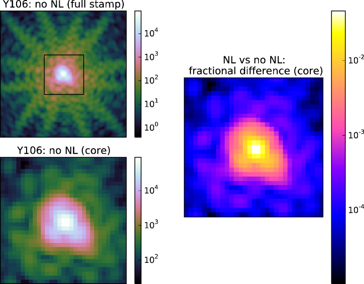
Figure 1: Example of the WFIRST PSF profiles in the Y106 band created by the galsim.wfirst.getPSF method. The profile is drawn on a postage stamp with a size of $1.5k\times 1.5k$ pixels ($k=64$) and a resolution of $p/N$, with $p=0.11$ arcseconds and $N=3$. Before drawing the profiles, they are first convolved with a pixel response of size $p$ and given a flux obtained through the use of the galsim.wfirst.getBandpasses (AB_zeropoint=True) routine at an AB magnitude of 18.3 (at an exposure time of 168.1 seconds). However, to preserve the correct response to NL, the higher-resolution image has $N^{2}$ more total flux. The NL effect is applied at the high-resolution pixel scale $p/N$, but the centroid of the profile is randomized within the native pixel scale $p$ (in this example the centroid and the pixel center coincide). The upper left panel shows the full postage stamp PSF image without the NL applied, while the lower left panel shows a zoom into the core (squared central region in upper left panel) of 30 by 30 high-resolution pixels. The right-hand side image shows the fractional difference between the PSF without the NL applied and a PSF with NL using $\beta_{0}$ for the model parameter.

The PSF profiles are drawn into squared postage stamps of size $1.5k$ pixels ($k=64$), large enough to ensure that most ($\sim 96\%$) of the total PSF flux is contained in the stamp. Each profile object was assigned a total flux of

$$f=b(\lambda)\times 10^{0.4(18.3-m)}\ \mathrm{e^{-}},$$ (4)

Eq. 4 gives the number of source counts per exposure, and $m$ represents the AB magnitude of the object for a given band. $b(\lambda)$ e^- is a baseline flux at AB magnitude $m=18.3$ for a exposure time of $168.1$.

We have neglected the main sources of noise that would affect the HLS—zodiacal background, thermal emission, and read noise—which would make all images slightly more nonlinear. Calculations performed with the WFIRST Exposure Time Calculator v.14 (Hirata et al., 2012) in weak lensing mode (ETC-WL) by Spergel et al. 2015 in the F184 band (a conservative case) show that the combined contribution due to these backgrounds sources would be approximately 130 $e^{-}$ per pixel for a $174$ seconds exposure (comparable to the $168.1$ seconds of exposure time assumed in this work), which creates negligible corrections in our simulations for a NL parameter $\beta$ of order $10^{-6}$.

Total and peak flux values at each filter per postage stamp are shown in Table 1. The peaks are upper limits estimated by assuming the PSF centroid is centered on a pixel. The brightest magnitude used was AB $m=18.3$, based on the peak value of the PSF profile in the Y106 band when rendered into a postage stamp at the native pixel scale and placed at the center of the pixel: $\sim 1.00237\times 10^{5}$ electrons, representing about $90\%$ of the typical full well depth in the pixels of the H4RG detectors—$\ \sim 1.1\times 10^{5}$ electrons. Recall that for each postage stamp, we select a centroid with coordinates randomly chosen from a uniform distributed across the native scale pixel. In addition, since NL is a function of signal, and since GalSim conserves total flux when changing pixel scales, the total flux in the higher resolution image must be multiplied by a factor of $N^{2}$ to preserve the appropriate response per pixel to this effect, correcting for the fact that the new image has a factor of $N^{2}$ more pixels than the one created at the native scale.

For simplicity of analysis, the postage stamps are noiseless and no other sensor effect is applied. After convolving the PSF profile with a pixel of the size of the native scale and rendering the image at the high-resolution scale, NL is applied by using Eq. 1.

Fig. 1 shows an example of the PSF profiles and postage stamps created for our simulations (in the Y106 band). The effect of NL (at the nominal $\beta_{0}$) is small, and the difference image reveals that the attenuation in the flux is of the order of a few percent, mainly for the larger signals found at the core of the PSF. Kannawadi et al. 2015 present more details on the galsim.wfirst module, along with examples of the PSF profiles that can be generated in all 6 WFIRST filters.

3.2 PSF size and shape measurement

The accurate determination of PSF properties such as size and ellipticity is crucial to avoid the propagation of systematic biases in cosmological parameters through the use of weak gravitational lensing (Paulin-Henriksson et al. 2008, Paulin-Henriksson et al. 2009, Massey et al. 2013, Cropper et al. 2013). In general, the problem of galaxy and PSF shape measurements for accurate weak lensing is non-trivial, and even when the PSF is perfectly known, shape measurement algorithms can introduce biases. Several shape measurements algorithms—ranging from model-fitting methods to particular combinations of weighted central moments and bayesian techniques—have been and are being investigated in order to produce accurate shear estimators that satisfy the requirements of current and future WL surveys (Mandelbaum et al., 2015).

To measure the profile shapes and size, we use the adaptive moments method (Bernstein and Jarvis 2002, Hirata and Seljak 2003).. Adaptive moments are effectively weighted by an elliptical Gaussian. At first they are calculated by computing moments weighted by a circular Gaussian with some arbitrary size. Then the output moments are used to define a new elliptical Gaussian that will act as a new weight function. The process is iteratively repeated until the output moments are the same as those of the weight function. The ellipticity $e=e_{1}+ie_{2}$ and size $R$ are then defined as

$$e_{1} =\frac{M_{xx}-M_{yy}}{M_{xx}+M_{yy}}$$ (5)

$$e_{2} =\frac{2M_{xy}}{M_{xx}+M_{yy}}$$ (6)

$$R =\det[\mathbf{M}]^{1/4}$$ (7)

where the centroid $\mathbf{\bar{x}}$ and moment matrix $\mathbf{M}$ of an image are defined as

$$\mathbf{\bar{x}} =\frac{\int d^{2}\mathbf{x}\ w(\mathbf{x})\mathbf{x}I(\mathbf{x})}{\int d^{2}\mathbf{x}\ w(\mathbf{x})I(\mathbf{x})}$$ (8)

$$M_{ij} =\frac{\int d^{2}\mathbf{x}\ (\mathbf{x}-\mathbf{\bar{x}})_{i}(\mathbf{x}-\mathbf{\bar{x}})_{j}w(\mathbf{x})I(\mathbf{x})}{\int d^{2}\mathbf{x}\ w(\mathbf{x})I(\mathbf{x})}$$ (9)

for an elliptical Gaussian weight function $w(\mathbf{x})$. We note that adaptive moments are particularly sensitive to the core of the PSF when the PSF profile is diffraction-limited, and therefore they should be particularly sensitive to NL effects.

3.3 Changes in size and ellipticity induced by NL

We quantify the effect of nonlinearity by measuring the fractional change in size and the absolute change in ellipticity of the PSF profiles, in the 4 filters of the HLS of WFIRST  and for several values of the NL model parameter $\beta$. We calculate the quantities $\Delta e_{1}$, $\Delta e_{2}$, and $\frac{\Delta R}{R}$, which are defined as the difference between the measured ellipticity or size after the effect (NL) is applied and the reference values measured before (represented by the subscript “$0$”) the application of NL:

$$\Delta e_{i} \equiv e_{i}-e_{i,0},\ \ \ i\in[1,2]$$ (10)

$$\frac{\Delta R}{R} \equiv\frac{{R}-R_{0}}{R_{0}}$$ (11)

In this way, we are less sensitive to the details (and possible biases) of the shape measurement algorithm, since we only care about relative changes induced by the detector effect.

The basic simulation process is summarized by the following steps:

• Create a WFIRST PSF surface brightness profile with a given flux as prescribed by Eq. 4, and convolve the PSF profile with a top-hat pixel response with the size of the native scale of the WFIRST FPA ($p=0.11$ arcseconds per pixel) to produce an effective PSF.

• Sample the effective PSF profile on a 2D grid to draw a noiseless postage stamp of size $1.5k$ by $1.5k$ ($k=64$) pixels at a higher resolution of of $p/N$, with $N=3$, and multiply the resulting image by $N^{2}$. In this step, NL is not yet applied, but it will be done so in a later step, so the flux still needs to be adjusted. The centroid of the profile is randomly selected from a uniform 2D distribution within the size of a native pixel.

• Create another image of the effective PSF at a higher resolution and with the flux adjusted as in step 2. Apply the nonlinearity to the postage stamps according to the transformation $I\mapsto I-\beta I^{2}$ (c.f. Eq. 1).

• Use the adaptive moments algorithm to measure the shape $e_{0}=(e_{1,0},e_{2,0})$ and size $R_{0}$ of the profile without NL to have as baseline reference.

• Measure the shape and size of the object with the sensor effect applied, and calculate the quantities $\Delta e_{1}$, $\Delta e_{2}$, and $\frac{\Delta R}{R}$, as defined in Eqs. 10 and 11.

• Repeat steps 1 to 5, averaging over 100 centroid realizations. The size and ellipticity values reported will be the mean and the standard deviation over these realizations (see Fig. 2 and Fig. 3).

• To study the impact of spatial variability in $\beta$, repeat steps 1 to 6 and assume that the model parameter $\beta$ for each high-resolution pixel can be drawn from a Gaussian distribution with a particular mean $\beta$ and variance $\sigma_{\beta}^{2}$. Over $M$ realizations (for a fixed centroid), calculate the dispersion values $\sigma_{\Delta e_{1}}$, $\sigma_{\Delta e_{2}}$, and $\sigma_{\Delta R/R}$ as a function of $\sigma_{\beta}$. In our simulations we use $M=100$ (see Fig. 4 and Fig. 5).

4 Results

4.1 Biases in ellipticity and size

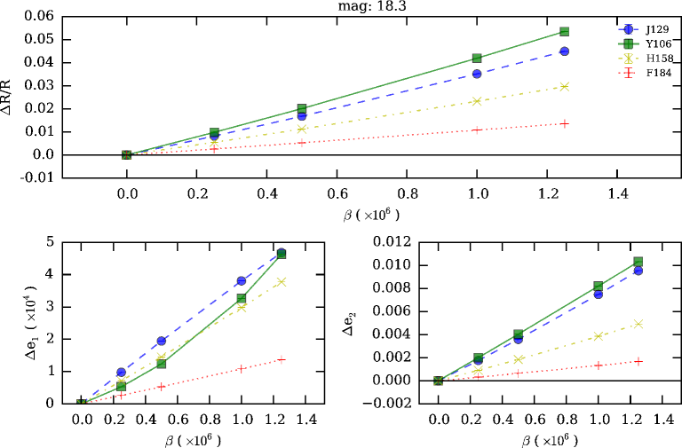
Figure 2: Fractional error in PSF size (upper panel) and absolute error in PSF ellipticity components (lower panels) as a function of the mean nonlinearity parameter $\beta$ for the WFIRST PSF, in four the four HSL filters (J129, Y106, H158, and F184), and an AB magnitude of 18.3 at 168.1 seconds of exposure time. Each point is the mean over 100 realizations of uniformly distributed random centroid shifts within the high resolution images ($N=3$). The standard deviations of the realizations are negligible.

Fig. 2 shows the fractional change in PSF size and the absolute error in PSF ellipticity as a function of the mean nonlinearity parameter $\beta$, for different bandpass filters at fixed AB magnitude of 18.3 in each band, consistent with the magnitude of nearly saturated stars in the HLS. We note that the flux in each band will depend on the particular stellar spectral energy distribution (SED), and we would need to specify a particular SED to go from one reference band to other bands. For simplicity, we are performing our calculations based on a grid of AB magnitudes in different filters.

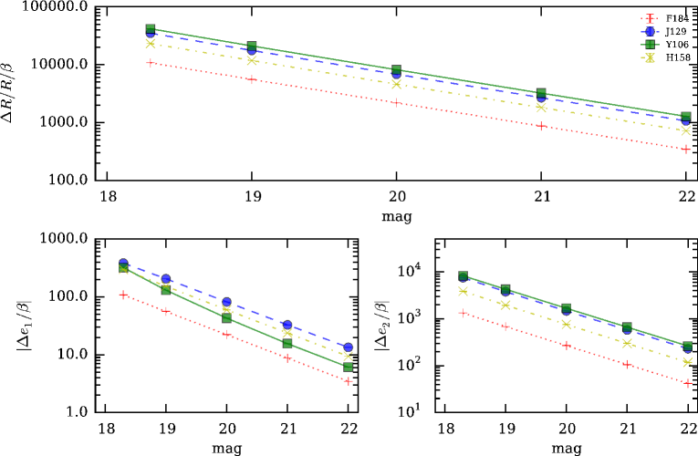
Figure 3: Fractional error in PSF size and absolute error in PSF ellipticity components normalized by the NL model parameter $\beta$, as a function of magnitude for the four HSL filters (J129, Y106, H158, and F184). The ordinate axis in each plot represents the slope of the linear relationships in Fig. 2, derived by linear fitting of points around the vicinity of $\beta_{0}$ in each curve of that figure.

In the H158 band, the mean nominal value of $\beta_{0}=5\times 10^{-7}/\mathrm{e^{-}}$ induces errors in the size and ellipticity of about $1\times 10^{-2}$ and $2\times 10^{-3}$ respectively, larger than the required values of $10^{-3}$ and $4.5\times 10^{-4}$ on the knowledge of the size and ellipticity of the PSF in order not to bias cosmological parameter inferences from WL experiments (Section1). As the $\beta$ parameter is increased, the amplitude of the errors increases approximately in a linear manner within the domain of $\beta$ values considered.

Since $\Delta R/R$ and $\Delta e$ are approximately linear in $\beta$, we can condense this information by simply plotting the slope for various filters and star magnitudes. This is shown in Fig. 3, which presents $\Delta R/R/\beta$ and $\Delta e/\beta$ (the slopes in Fig. 2) vs $m$ for each of the four filters of the HLS. From Fig. 3, it is possible to estimate the precision to which $\beta$ would have to be calibrated in order to limit the relative size and ellipticity bias of a star with a given magnitude. In particular, letting $(\beta-\beta_{0})/\beta_{0}\equiv\Delta\beta/\beta_{0}$ represent the fractional error in the measurement of a given value of $\beta_{0}$, we have:

$$\frac{\Delta R/R}{\Delta\beta}=c\ \ \ \ \Rightarrow\ \ \ \ \frac{\Delta\beta}{\beta_{0}}=\frac{\Delta R/R}{c\beta_{0}}$$ (12)

In Eq. 12, $c$ represents the ordinate value in Fig. 3 for a given magnitude, and we have replaced $\Delta R/R/\beta$ by $\Delta R/R/\Delta\beta$ since the linearity in the bias in $\Delta R/R$ and $\Delta e$ vs $\beta$ for all magnitudes makes the choice of the expansion point of the approximation by Taylor expansion unimportant (i.e., it does not matter if the expansion is around $\beta=0$ or $\beta=\beta_{0}$). An analogous equation to Eq. 12 can be written for the error in the ellipticity if $\Delta R/R$ is replaced by $\Delta e$.

Under these conditions, Fig. 3 shows that for the brightest stars in our range, to limit the bias of $\Delta R/R$ ($\Delta e$) in the H158 band to $10^{-4}$ ($4.7\times 10^{-5}$)—about $10\%$ of the estimated WFIRST error budgets, $\beta$ must be calibrated to $\sim 1\%$ ($\sim 2.4\%$) (using $c\sim 2\times 10^{4}$ at $m=18.3$ from the upper panel of Fig. 3, $c\sim 4000$ at $m=18.3$ from the lower right panel of the same figure, and $\beta_{0}=5\times 10^{-7}$). Alternatively, this calculation can be used to convert between NL calibration requirements, shape measurement error requirements, and the minimum useable star magnitude: given any two of these, we can obtain the third. E.g., if NL calibration precision reaches some practical limit, then given a tolerance on shape measurement error, one can find the star magnitude for which the shape measurement bias due to NL matches the tolerance (brighter stars cannot be used to measure the PSF). Our choice of error tolerance here is only for illustration, and Eq. 12 and Fig. 3 should be used to derive detector requirements once true PSF requirements are known.

The trends in Fig. 3 are clearly well-described by a power law with a common slope for the various filters. We fit a function only to the PSF size trend since it will be a more robust characteristic of the survey, whereas ellipticity can have relatively wide spatial variations. For a power law of the form

$$\frac{\Delta R/R}{\beta}=A_{\text{F}}10^{B_{\text{F}}(m-m_{0})}\ (m_{0}=20),$$ (13)

the parameters $A_{\text{F}}$ and $B_{\text{F}}$ for each filter F are listed in Table 2.

4.2 Impacts of spatial variability of $\beta$

We also studied the impact on $\Delta e$ and $\Delta R/R$ due to the dispersion in the $\beta$ parameter. Due to non-uniformities in fabrication, each pixel can have a different NL coefficient, and biases in the measurement of PSF properties could be introduced if a mean response curve is used to calibrate NL instead of a single curve per pixel. Fig. 4 shows the dispersion over $M=100$ realizations (for a fixed centroid) in the metrics $\Delta e_{1}$, $\Delta e_{2}$, and $\Delta R/R$ as a function of the standard deviation $\sigma_{\beta_{0}}$, assuming that the coefficient $\beta$ is drawn from a distribution of the form $\mathcal{N}\sim(\beta_{0},\sigma_{\beta_{0}})$. We have verified that the mean value of the metrics over all the realizations are consistent with the case where a fixed $\beta_{0}$ is considered, and therefore our stochastic beta model simply introduces scatter around the shape measurement biases computed in Section 4.1.

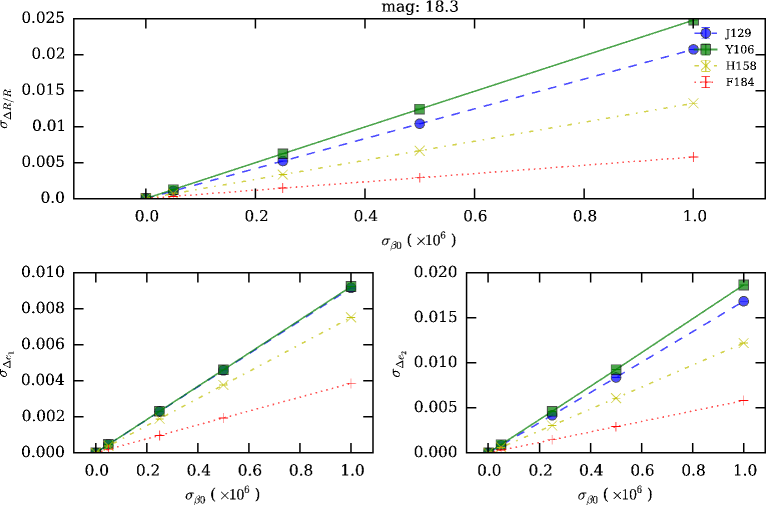
Figure 4: Impact of spatial variability in the $\beta_{0}$ parameter, quantified as the standard deviation over $M=100$ realizations (for a fixed centroid) in $\Delta e_{1}$, $\Delta e_{2}$, and $\Delta R/R$ as a function of the standard deviation $\sigma_{\beta_{0}}$. The source magnitude is fixed at 18.3.

We found that the results in Fig. 4 are insensitive to the nominal $\beta$ and therefore, in general, $\sigma_{\beta}$ can be treated as an error on $\beta$ estimation. The linear relationships in Fig. 4 also allows us to plot the slope of each curve for different magnitudes, as was done in Fig. 3, and therefore analogous equations to Eq. 12 can be used to convert between the dispersion in errors on $\beta$ and the dispersions of errors in size and ellipticity measurements. This computation may also be useful for deriving calibration requirements, although weak lensing analyses are much more sensitive to shape measurement biases than to small random errors. The results are shown in Fig. 5. We also fitted a model of the form

$$\frac{\sigma_{\Delta R/R}}{\sigma_{\beta}}=A_{\text{F}}10^{B_{\text{F}}(m-m_{0})}\ (m_{0}=20)$$ (14)

for the PSF size trends in Fig. 5, as was done above for Fig. 3 (c.f., Eq. 13). The fit parameters are presented in Table 2 as well.

Band	size bias (Fig. 3)		size scatter (Fig. 5)
	$A_{\text{F}}$	$B_{\text{F}}$	$\ A_{\text{F}}$	$B_{\text{F}}$
Y106	8322	-0.4086	5057	-0.4045
J129	6958	-0.4089	4215	-0.4050
H158	4668	-0.4069	2711	-0.4038
F184	2209	-0.4035	1194	-0.4018

Table 2: Parameters resulting from fitting the curves in the upper panel of Figs. 3 and 5 to power-law functions of the form $\Delta R/R/\beta=A_{\text{F}}\ 10^{B_{\text{F}}(m-20)}$ and $\sigma_{\Delta R/R}/\sigma_{\beta}=A_{\text{F}}\ 10^{B_{\text{F}}(m-20)}$, respectively.

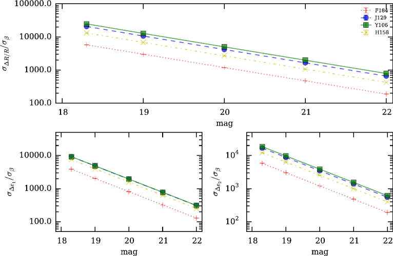
Figure 5: Standard deviation of the fractional error in PSF size and of the absolute error in PSF ellipticity components normalized by the error in the NL parameter $\sigma_{\beta}$, as a function of magnitude for the four HSL filters (J129, Y106, H158, and F184).

5 Conclusion

We have used the WFIRST module in GalSim to study the impact on PSF measurement for weak lensing science due to the nonlinearity in the conversion of charge to voltage in near-infrared hybrid CMOS detectors (such as those that will be used in the Wide Field Imager of the WFIRST mission). The PSF profiles created by the galsim.wfirst module posses several of the design characteristics of the expected PSF of the mission, such as optical aberrations and pixel scale. The module can also be used to assign the PSF profiles fluxes per pixel consistent with the expected brightness of the HLS.

Voltage nonlinearity—as studied in this work—encompasses the linearity due to the shrinking of the depletion region at the p-n junction as charge accumulates, and the deviation from linearity originating in the multiplexer gain. It depends on the total integrated signal (fluence), and it is more dominant at high signals than other types of nonlinearity such as reciprocity failure, which dominates at lower signals. As such, NL will tend to depresses the flux in the core of the PSF relative to the wings in bright stars that are usually used for PSF estimation, introducing errors when deconvolving the PSF at the interpolated galaxy positions.

To model NL, we have used a single, one-parameter transfer function quadratic in the charge $Q$ (Eq. 1). We have studied the consequences of NL in isolation by using the relationship in Eq.1, not considering other sensor effects, and neglecting sources of noise such as zodiacal background, thermal emission, and read noise (which would produce a negligible contribution). We have used the metrics $\Delta R/R$ and $\Delta e$ to assess the impact of NL on PSF size and ellipticity, which have to be controlled to $\sim O(10^{-4})$ or better, for different values of the parameter space at hand ($\beta$, PSF magnitude, and bandpass filters to be used in WFIRST WL analyses). We have also studied the effects of spatial variation of the $\beta$ coefficient along the pixel array, by assuming that it follows a Gaussian distribution.

For the nominal value $\beta_{0}$ assumed in this work, we find that NL induces errors in PSF size and shape larger to what is tolerable by accurate WL measurements. For an example set of assumed requirements on PSF size and ellipticity ($10^{-4}$ and $4.7\times 10^{-5}$, respectively), we find that $\beta$ should be calibrated to about $1\%$ to $2.4\%$ (H158 band). However, the results derived in this study (Eq. 12, Fig. 3, and Fig. 5) can be used to derive requirements on NL for the WFIRST detectors for a different set of tolerances on PSF properties. It is important to note that new measurements on the actual H4RG detector that will be used by the WFIRST imager will have to be performed in order to determine the mean value of $\beta$ and its dispersion.

Nonlinearity measurements are usually performed by looking at signal as a function of exposure time at a constant flux (and subtracting dark frames at the appropriate times), which is sensible to any gain dependence on fluence. These measurements are normally subject to other effects such as inaccuracies in the readout time, persistence, reciprocity failure, and time-dependent changes in the electronic offset due to self-heating effects in the multiplexer. Despite these challenges, the mean non-linearity signal can usually be characterized to a precision of 5–10$\%$. Thus it is not obvious that a typical NL calibration program will be sufficient for WL with WFIRST without more careful study and error budgeting. To ensure that voltage nonlinearity in the WFIRST H4RG detectors can be calibrated to the levels demanded by WL science, NL characterization will be crucial through the use of facilities such as the Detector Characterization Laboratory for rigorous calibration studies and the Precision Projector Laboratory (PPL, Seshadri et al. 2013, Shapiro et al. 2013) for validating the impact of NL on shape measurement.

We thank Chris Hirata, Jeff Kruk, Dave Content, and the WFIRST detector requirements working group for useful discussions. AAP is supported by the Jet Propulsion Laboratory. CS and JR are being supported in part by the Jet Propulsion Laboratory. The research was carried out at the Jet Propulsion Laboratory, California Institute of Technology, under a contract with the National Aeronautics and Space Administration.

© 2016. All rights reserved.

References

- Albrecht et al. [2006] A. Albrecht, G. Bernstein, R. Cahn, W. L. Freedman, J. Hewitt, W. Hu, J. Huth, M. Kamionkowski, E. W. Kolb, L. Knox, J. C. Mather, S. Staggs, and N. B. Suntzeff. Report of the Dark Energy Task Force. ArXiv Astrophysics e-prints, September 2006.
- Alsing et al. [2016] J. Alsing, A. Heavens, A. H. Jaffe, A. Kiessling, B. Wandelt, and T. Hoffmann. Hierarchical cosmic shear power spectrum inference. MNRAS, 455:4452–4466, February 2016. 10.1093/mnras/stv2501.
- Amara and Réfrégier [2008] A. Amara and A. Réfrégier. Systematic bias in cosmic shear: extending the Fisher matrix. MNRAS, 391:228–236, November 2008. 10.1111/j.1365-2966.2008.13880.x.
- Beletic et al. [2008] James W. Beletic, Richard Blank, David Gulbransen, Donald Lee, Markus Loose, Eric C. Piquette, Thomas Sprafke, William E. Tennant, Majid Zandian, and Joseph Zino. Teledyne imaging sensors: infrared imaging technologies for astronomy and civil space, 2008.
- Bernstein and Armstrong [2014] G. M. Bernstein and R. Armstrong. Bayesian lensing shear measurement. MNRAS, 438:1880–1893, February 2014. 10.1093/mnras/stt2326.
- Bernstein and Jarvis [2002] G. M. Bernstein and M. Jarvis. Shapes and Shears, Stars and Smears: Optimal Measurements for Weak Lensing. AJ, 123:583–618, February 2002. 10.1086/338085.
- Bernstein et al. [2015] G. M. Bernstein, R. Armstrong, C. Krawiec, and M. C. March. An accurate and practical method for inference of weak gravitational lensing from galaxy images. ArXiv e-prints, August 2015.
- Bertin [2006] E. Bertin. Automatic Astrometric and Photometric Calibration with SCAMP. In C. Gabriel, C. Arviset, D. Ponz, and S. Enrique, editors, Astronomical Data Analysis Software and Systems XV, volume 351 of Astronomical Society of the Pacific Conference Series, page 112, July 2006.
- Biesiadzinski et al. [2011] T. Biesiadzinski, W. Lorenzon, R. Newman, M. Schubnell, G. Tarlé, and C. Weaverdyck. Measurement of Reciprocity Failure in Near-Infrared Detectors. PASP, 123:179–186, February 2011. 10.1086/658282.
- Bohlin et al. [2005] R. C. Bohlin, D. J. Lindler, and A. Riess. Grism Sensitivities and Apparent Non-Linearity. Technical report, May 2005.
- Cropper et al. [2013] M. Cropper, H. Hoekstra, T. Kitching, R. Massey, J. Amiaux, L. Miller, Y. Mellier, J. Rhodes, B. Rowe, S. Pires, C. Saxton, and R. Scaramella. Defining a weak lensing experiment in space. MNRAS, 431:3103–3126, June 2013. 10.1093/mnras/stt384.
- Diehl and Dark Energy Survey Collaboration [2012] T. Diehl and Dark Energy Survey Collaboration. The Dark Energy Survey Camera (DECam). Physics Procedia, 37:1332–1340, 2012. 10.1016/j.phpro.2012.02.472.
- Fruchter [2011] A. S. Fruchter. A New Method for Band-limited Imaging with Undersampled Detectors. PASP, 123:497–502, April 2011. 10.1086/659313.
- Fruchter and Hook [2002] A. S. Fruchter and R. N. Hook. Drizzle: A Method for the Linear Reconstruction of Undersampled Images. PASP, 114:144–152, February 2002. 10.1086/338393.
- Girardi et al. [2012] L. Girardi, M. Barbieri, M. A. T. Groenewegen, P. Marigo, A. Bressan, H. J. Rocha-Pinto, B. X. Santiago, J. I. B. Camargo, and L. N. da Costa. TRILEGAL, a TRIdimensional modeL of thE GALaxy: Status and Future. Astrophysics and Space Science Proceedings, 26:165, 2012. 10.1007/978-3-642-18418-5_17.
- Green et al. [2012] J. Green, P. Schechter, C. Baltay, R. Bean, D. Bennett, R. Brown, C. Conselice, M. Donahue, X. Fan, B. S. Gaudi, C. Hirata, J. Kalirai, T. Lauer, B. Nichol, N. Padmanabhan, S. Perlmutter, B. Rauscher, J. Rhodes, T. Roellig, D. Stern, T. Sumi, A. Tanner, Y. Wang, D. Weinberg, E. Wright, N. Gehrels, R. Sambruna, W. Traub, J. Anderson, K. Cook, P. Garnavich, L. Hillenbrand, Z. Ivezic, E. Kerins, J. Lunine, P. McDonald, M. Penny, M. Phillips, G. Rieke, A. Riess, R. van der Marel, R. K. Barry, E. Cheng, D. Content, R. Cutri, R. Goullioud, K. Grady, G. Helou, C. Jackson, J. Kruk, M. Melton, C. Peddie, N. Rioux, and M. Seiffert. Wide-Field InfraRed Survey Telescope (WFIRST) Final Report. ArXiv e-prints, August 2012.
- Gruen et al. [2015] D. Gruen, G. M. Bernstein, M. Jarvis, B. Rowe, V. Vikram, A. A. Plazas, and S. Seitz. Characterization and correction of charge-induced pixel shifts in DECam. Journal of Instrumentation, 10:C05032, May 2015. 10.1088/1748-0221/10/05/C05032.
- Hilbert [2004] B. Hilbert. Non-Linearity Correction Algorithm for the WFC3 IR Channel. Technical report, May 2004.
- Hilbert [2008] B. Hilbert. WFC3 TV3 Testing: IR Channel Nonlinearity Correction. Technical report, 2008.
- Hilbert [2014] B. Hilbert. Updated non-linearity calibration method for WFC3/IR. Technical report, July 2014.
- Hirata and Seljak [2003] C. Hirata and U. Seljak. Shear calibration biases in weak-lensing surveys. MNRAS, 343:459–480, August 2003. 10.1046/j.1365-8711.2003.06683.x.
- Hirata et al. [2012] C. M. Hirata, N. Gehrels, J.-P. Kneib, J. Kruk, J. Rhodes, Y. Wang, and J. Zoubian. The WFIRST Galaxy Survey Exposure Time Calculator. ArXiv e-prints, April 2012.
- Hoekstra and Jain [2008] H. Hoekstra and B. Jain. Weak gravitational lensing and its cosmological applications. Annual Review of Nuclear and Particle Systems, 58:99–123, 2008.
- Huterer et al. [2006] D. Huterer, M. Takada, G. Bernstein, and B. Jain. Systematic errors in future weak-lensing surveys: requirements and prospects for self-calibration. MNRAS, 366:101–114, February 2006. 10.1111/j.1365-2966.2005.09782.x.
- Ivezic et al. [2008] Z. Ivezic, J. A. Tyson, B. Abel, E. Acosta, R. Allsman, Y. AlSayyad, S. F. Anderson, J. Andrew, R. Angel, G. Angeli, R. Ansari, P. Antilogus, K. T. Arndt, P. Astier, E. Aubourg, T. Axelrod, D. J. Bard, J. D. Barr, A. Barrau, J. G. Bartlett, B. J. Bauman, S. Beaumont, A. C. Becker, J. Becla, C. Beldica, S. Bellavia, G. Blanc, R. D. Blandford, J. S. Bloom, J. Bogart, K. Borne, J. F. Bosch, D. Boutigny, W. N. Brandt, M. E. Brown, J. S. Bullock, P. Burchat, D. L. Burke, G. Cagnoli, D. Calabrese, S. Chandrasekharan, S. Chesley, E. C. Cheu, J. Chiang, C. F. Claver, A. J. Connolly, K. H. Cook, A. Cooray, K. R. Covey, C. Cribbs, W. Cui, R. Cutri, G. Daubard, G. Daues, F. Delgado, S. Digel, P. Doherty, R. Dubois, G. P. Dubois-Felsmann, J. Durech, M. Eracleous, H. Ferguson, J. Frank, M. Freemon, E. Gangler, E. Gawiser, J. C. Geary, P. Gee, M. Geha, R. R. Gibson, D. K. Gilmore, T. Glanzman, I. Goodenow, W. J. Gressler, P. Gris, A. Guyonnet, P. A. Hascall, J. Haupt, F. Hernandez, C. Hogan, D. Huang, M. E. Huffer, W. R. Innes, S. H. Jacoby, B. Jain, J. Jee, J. G. Jernigan, D. Jevremovic, K. Johns, R. L. Jones, C. Juramy-Gilles, M. Juric, S. M. Kahn, J. S. Kalirai, N. Kallivayalil, B. Kalmbach, J. P. Kantor, M. M. Kasliwal, R. Kessler, D. Kirkby, L. Knox, I. Kotov, V. L. Krabbendam, S. Krughoff, P. Kubanek, J. Kuczewski, S. Kulkarni, R. Lambert, L. Le Guillou, D. Levine, M. Liang, K. Lim, C. Lintott, R. H. Lupton, A. Mahabal, P. Marshall, S. Marshall, M. May, R. McKercher, M. Migliore, M. Miller, D. J. Mills, D. G. Monet, M. Moniez, D. R. Neill, J. Nief, A. Nomerotski, M. Nordby, P. O’Connor, J. Oliver, S. S. Olivier, K. Olsen, S. Ortiz, R. E. Owen, R. Pain, J. R. Peterson, C. E. Petry, F. Pierfederici, S. Pietrowicz, R. Pike, P. A. Pinto, R. Plante, S. Plate, P. A. Price, M. Prouza, V. Radeka, J. Rajagopal, A. Rasmussen, N. Regnault, S. T. Ridgway, S. Ritz, W. Rosing, C. Roucelle, M. R. Rumore, S. Russo, A. Saha, B. Sassolas, T. L. Schalk, R. H. Schindler, D. P. Schneider, G. Schumacher, J. Sebag, G. H. Sembroski, L. G. Seppala, I. Shipsey, N. Silvestri, J. A. Smith, R. C. Smith, M. A. Strauss, C. W. Stubbs, D. Sweeney, A. Szalay, P. Takacs, J. J. Thaler, R. Van Berg, D. Vanden Berk, K. Vetter, F. Virieux, B. Xin, L. Walkowicz, C. W. Walter, D. L. Wang, M. Warner, B. Willman, D. Wittman, S. C. Wolff, W. M. Wood-Vasey, P. Yoachim, H. Zhan, and for the LSST Collaboration. LSST: from Science Drivers to Reference Design and Anticipated Data Products. ArXiv e-prints, May 2008.
- Jarvis [2014] M Jarvis. Challenges for precision shape measurements. Journal of Instrumentation, 9(03):C03017, 2014. URL http://stacks.iop.org/1748-0221/9/i=03/a=C03017.
- Jarvis et al. [2015] M. Jarvis, E. Sheldon, J. Zuntz, T. Kacprzak, S. L. Bridle, A. Amara, R. Armstrong, M. R. Becker, G. M. Bernstein, C. Bonnett, C. Chang, R. Das, J. P. Dietrich, A. Drlica-Wagner, T. F. Eifler, C. Gangkofner, D. Gruen, M. Hirsch, E. M. Huff, B. Jain, S. Kent, D. Kirk, N. MacCrann, P. Melchior, A. A. Plazas, A. Refregier, B. Rowe, E. S. Rykoff, S. Samuroff, C. Sánchez, E. Suchyta, M. A. Troxel, V. Vikram, T. Abbott, F. B. Abdalla, S. Allam, J. Annis, A. Benoit-Lévy, E. Bertin, D. Brooks, E. Buckley-Geer, D. L. Burke, D. Capozzi, A. Carnero Rosell, M. Carrasco Kind, J. Carretero, F. J. Castander, M. Crocce, C. E. Cunha, C. B. D’Andrea, L. N. da Costa, D. L. DePoy, S. Desai, H. T. Diehl, P. Doel, A. Fausti Neto, B. Flaugher, P. Fosalba, J. Frieman, E. Gaztanaga, D. W. Gerdes, R. A. Gruendl, G. Gutierrez, K. Honscheid, D. J. James, K. Kuehn, N. Kuropatkin, O. Lahav, T. S. Li, M. Lima, M. March, P. Martini, R. Miquel, J. J. Mohr, E. Neilsen, B. Nord, R. Ogando, K. Reil, A. K. Romer, A. Roodman, M. Sako, E. Sanchez, V. Scarpine, M. Schubnell, I. Sevilla-Noarbe, R. C. Smith, M. Soares-Santos, F. Sobreira, M. E. C. Swanson, G. Tarle, J. Thaler, D. Thomas, A. R. Walker, and R. H. Wechsler. The DES Science Verification Weak Lensing Shear Catalogs. ArXiv e-prints, July 2015.
- Kannawadi et al. [2015] A. Kannawadi, C. A. Shapiro, R. Mandelbaum, C. M. Hirata, J. W. Kruk, and J. D. Rhodes. The Impact of Interpixel Capacitance on WFIRST PSFs. ArXiv e-prints, December 2015.
- Kilbinger [2015] M. Kilbinger. Cosmology with cosmic shear observations: a review. Reports on Progress in Physics, 78(8):086901, July 2015. 10.1088/0034-4885/78/8/086901.
- Kuijken et al. [2015] K. Kuijken, C. Heymans, H. Hildebrandt, R. Nakajima, T. Erben, J. T. A. de Jong, M. Viola, A. Choi, H. Hoekstra, L. Miller, E. van Uitert, A. Amon, C. Blake, M. Brouwer, A. Buddendiek, I. F. Conti, M. Eriksen, A. Grado, J. Harnois-Déraps, E. Helmich, R. Herbonnet, N. Irisarri, T. Kitching, D. Klaes, F. La Barbera, N. Napolitano, M. Radovich, P. Schneider, C. Sifón, G. Sikkema, P. Simon, A. Tudorica, E. Valentijn, G. Verdoes Kleijn, and L. van Waerbeke. Gravitational lensing analysis of the Kilo-Degree Survey. MNRAS, 454:3500–3532, December 2015. 10.1093/mnras/stv2140.
- Lauer [1999a] T. R. Lauer. The Photometry of Undersampled Point-Spread Functions. PASP, 111:1434–1443, November 1999a. 10.1086/316460.
- Lauer [1999b] T. R. Lauer. Combining Undersampled Dithered Images. PASP, 111:227–237, February 1999b. 10.1086/316319.
- Laureijs et al. [2011] R. Laureijs, J. Amiaux, S. Arduini, J. . Auguères, J. Brinchmann, R. Cole, M. Cropper, C. Dabin, L. Duvet, A. Ealet, and et al. Euclid Definition Study Report. ArXiv e-prints, October 2011.
- Mandelbaum [2015] R. Mandelbaum. Instrumental systematics and weak gravitational lensing. Journal of Instrumentation, 10(05):C05017, 2015. URL http://stacks.iop.org/1748-0221/10/i=05/a=C05017.
- Mandelbaum et al. [2015] R. Mandelbaum, B. Rowe, R. Armstrong, D. Bard, E. Bertin, J. Bosch, D. Boutigny, F. Courbin, W. A. Dawson, A. Donnarumma, I. Fenech Conti, R. Gavazzi, M. Gentile, M. S. S. Gill, D. W. Hogg, E. M. Huff, M. J. Jee, T. Kacprzak, M. Kilbinger, T. Kuntzer, D. Lang, W. Luo, M. C. March, P. J. Marshall, J. E. Meyers, L. Miller, H. Miyatake, R. Nakajima, F. M. Ngolé Mboula, G. Nurbaeva, Y. Okura, S. Paulin-Henriksson, J. Rhodes, M. D. Schneider, H. Shan, E. S. Sheldon, M. Simet, J.-L. Starck, F. Sureau, M. Tewes, K. Zarb Adami, J. Zhang, and J. Zuntz. GREAT3 results - I. Systematic errors in shear estimation and the impact of real galaxy morphology. MNRAS, 450:2963–3007, July 2015. 10.1093/mnras/stv781.
- Marks [2009] R. J. Marks. Handbook of Fourier Analysis and Its Applications. Oxford University Press, 1 edition, 2009.
- Massey et al. [2013] R. Massey, H. Hoekstra, T. Kitching, J. Rhodes, M. Cropper, J. Amiaux, D. Harvey, Y. Mellier, M. Meneghetti, L. Miller, S. Paulin-Henriksson, S. Pires, R. Scaramella, and T. Schrabback. Origins of weak lensing systematics, and requirements on future instrumentation (or knowledge of instrumentation). MNRAS, 429:661–678, February 2013. 10.1093/mnras/sts371.
- McCaughrean [1987] M. J. McCaughrean. The astronomical application of infrared array detectors. PhD thesis, Edinburgh Univ. (Scotland)., 1987.
- McCullough [2008] P. McCullough. Inter-pixel capacitance: prospects for deconvolution. Technical report, August 2008.
- Meyers and Burchat [2014] J E Meyers and P R Burchat. Impact of chromatic effects on galaxy shape measurements. Journal of Instrumentation, 9(03):C03037, 2014. URL http://stacks.iop.org/1748-0221/9/i=03/a=C03037.
- Miller et al. [2013] L. Miller, C. Heymans, T. D. Kitching, L. van Waerbeke, T. Erben, H. Hildebrandt, H. Hoekstra, Y. Mellier, B. T. P. Rowe, J. Coupon, J. P. Dietrich, L. Fu, J. Harnois-Déraps, M. J. Hudson, M. Kilbinger, K. Kuijken, T. Schrabback, E. Semboloni, S. Vafaei, and M. Velander. Bayesian galaxy shape measurement for weak lensing surveys - III. Application to the Canada-France-Hawaii Telescope Lensing Survey. MNRAS, 429:2858–2880, March 2013. 10.1093/mnras/sts454.
- Miyazaki et al. [2012] S. Miyazaki, Y. Komiyama, H. Nakaya, Y. Kamata, Y. Doi, T. Hamana, H. Karoji, H. Furusawa, S. Kawanomoto, T. Morokuma, Y. Ishizuka, K. Nariai, Y. Tanaka, F. Uraguchi, Y. Utsumi, Y. Obuchi, Y. Okura, M. Oguri, T. Takata, D. Tomono, T. Kurakami, K. Namikawa, T. Usuda, H. Yamanoi, T. Terai, H. Uekiyo, Y. Yamada, M. Koike, H. Aihara, Y. Fujimori, S. Mineo, H. Miyatake, N. Yasuda, J. Nishizawa, T. Saito, M. Tanaka, T. Uchida, N. Katayama, S.-Y. Wang, H.-Y. Chen, R. Lupton, C. Loomis, S. Bickerton, P. Price, J. Gunn, H. Suzuki, Y. Miyazaki, M. Muramatsu, K. Yamamoto, M. Endo, Y. Ezaki, N. Itoh, Y. Miwa, H. Yokota, T. Matsuda, R. Ebinuma, and K. Takeshi. Hyper Suprime-Cam. In Society of Photo-Optical Instrumentation Engineers (SPIE) Conference Series, volume 8446 of Society of Photo-Optical Instrumentation Engineers (SPIE) Conference Series, page 0, September 2012. 10.1117/12.926844.
- Niemi et al. [2015] S.-M. Niemi, M. Cropper, M. Szafraniec, and T. Kitching. Measuring a charge-coupled device point spread function. Euclid visible instrument CCD273-84 PSF performance. Experimental Astronomy, 39:207–231, June 2015. 10.1007/s10686-015-9440-7.
- Pasquale et al. [2014] Jeffrey Kruk David Vaughnn Qian Gong Joseph Howard Alden Jurling Len Seals Eric Mentzell Nerses Armani Gary Kuan Pasquale et al., David Content. Optical design of the wfirst-afta wide-field instrument. Proc. SPIE 9293, International Optical Design Conference 2014, 2014.
- Paulin-Henriksson et al. [2008] S. Paulin-Henriksson, A. Amara, L. Voigt, A. Refregier, and S. L. Bridle. Point spread function calibration requirements for dark energy from cosmic shear. A&A, 484:67–77, June 2008. 10.1051/0004-6361:20079150.
- Paulin-Henriksson et al. [2009] S. Paulin-Henriksson, A. Refregier, and A. Amara. Optimal point spread function modeling for weak lensing: complexity and sparsity. A&A, 500:647–655, June 2009. 10.1051/0004-6361/200811061.
- Plazas et al. [2014] A. A. Plazas, G. M. Bernstein, and E. S. Sheldon. On-Sky Measurements of the Transverse Electric Fields’ Effects in the Dark Energy Camera CCDs. PASP, 126:750–760, September 2014. 10.1086/677682.
- Prod’homme et al. [2014] T. Prod’homme, P. Verhoeve, R. Kohley, A. Short, and N. Boudin. A comparative study of charge transfer inefficiency value and trap parameter determination techniques making use of an irradiated ESA-Euclid prototype CCD. In High Energy, Optical, and Infrared Detectors for Astronomy VI, volume 9154 of Proc. SPIE, page 915409, July 2014. 10.1117/12.2054862.
- Réfrégier [2003] A. Réfrégier. Weak gravitational lensing by large-scale structure. Annual Review of Astronomy and Astrophysics, 41:645–668, 2003.
- Rhodes et al. [2007] J. D. Rhodes, R. J. Massey, J. Albert, N. Collins, R. S. Ellis, C. Heymans, J. P. Gardner, J.-P. Kneib, A. Koekemoer, A. Leauthaud, Y. Mellier, A. Refregier, J. E. Taylor, and L. Van Waerbeke. The Stability of the Point-Spread Function of the Advanced Camera for Surveys on the Hubble Space Telescope and Implications for Weak Gravitational Lensing. ApJS, 172:203–218, September 2007. 10.1086/516592.
- Rowe et al. [2011] B. Rowe, C. Hirata, and J. Rhodes. Optimal Linear Image Combination. ApJ, 741:46, November 2011. 10.1088/0004-637X/741/1/46.
- Rowe et al. [2015] B. T. P. Rowe, M. Jarvis, R. Mandelbaum, G. M. Bernstein, J. Bosch, M. Simet, J. E. Meyers, T. Kacprzak, R. Nakajima, J. Zuntz, H. Miyatake, J. P. Dietrich, R. Armstrong, P. Melchior, and M. S. S. Gill. GALSIM: The modular galaxy image simulation toolkit. Astronomy and Computing, 10:121–150, April 2015. 10.1016/j.ascom.2015.02.002.
- Schneider et al. [2015] M. D. Schneider, D. W. Hogg, P. J. Marshall, W. A. Dawson, J. Meyers, D. J. Bard, and D. Lang. Hierarchical Probabilistic Inference of Cosmic Shear. ApJ, 807:87, July 2015. 10.1088/0004-637X/807/1/87.
- Seshadri et al. [2013] S. Seshadri, C. Shapiro, T. Goodsall, J. Fucik, C. Hirata, J. D. Rhodes, B. T. P. Rowe, and R. M. Smith. Initial Results from a Laboratory Emulation of Weak Gravitational Lensing Measurements. PASP, 125:1065–1086, September 2013. 10.1086/673318.
- Shapiro et al. [2013] C. Shapiro, B. T. P. Rowe, T. Goodsall, C. Hirata, J. Fucik, J. Rhodes, S. Seshadri, and R. Smith. Weak Gravitational Lensing Systematics from Image Combination. PASP, 125:1496–1513, December 2013. 10.1086/674415.
- Smith et al. [2008] R. M. Smith, M. Zavodny, G. Rahmer, and M. Bonati. A theory for image persistence in HgCdTe photodiodes. In Society of Photo-Optical Instrumentation Engineers (SPIE) Conference Series, volume 7021 of Society of Photo-Optical Instrumentation Engineers (SPIE) Conference Series, page 0, July 2008. 10.1117/12.789372.
- Spergel et al. [2013] D. Spergel, N. Gehrels, J. Breckinridge, M. Donahue, A. Dressler, B. S. Gaudi, T. Greene, O. Guyon, C. Hirata, J. Kalirai, N. J. Kasdin, W. Moos, S. Perlmutter, M. Postman, B. Rauscher, J. Rhodes, Y. Wang, D. Weinberg, J. Centrella, W. Traub, C. Baltay, J. Colbert, D. Bennett, A. Kiessling, B. Macintosh, J. Merten, M. Mortonson, M. Penny, E. Rozo, D. Savransky, K. Stapelfeldt, Y. Zu, C. Baker, E. Cheng, D. Content, J. Dooley, M. Foote, R. Goullioud, K. Grady, C. Jackson, J. Kruk, M. Levine, M. Melton, C. Peddie, J. Ruffa, and S. Shaklan. Wide-Field InfraRed Survey Telescope-Astrophysics Focused Telescope Assets WFIRST-AFTA Final Report. ArXiv e-prints, May 2013.
- Spergel et al. [2015] D. Spergel, N. Gehrels, C. Baltay, D. Bennett, J. Breckinridge, M. Donahue, A. Dressler, B. S. Gaudi, T. Greene, O. Guyon, C. Hirata, J. Kalirai, N. J. Kasdin, B. Macintosh, W. Moos, S. Perlmutter, M. Postman, B. Rauscher, J. Rhodes, Y. Wang, D. Weinberg, D. Benford, M. Hudson, W.-S. Jeong, Y. Mellier, W. Traub, T. Yamada, P. Capak, J. Colbert, D. Masters, M. Penny, D. Savransky, D. Stern, N. Zimmerman, R. Barry, L. Bartusek, K. Carpenter, E. Cheng, D. Content, F. Dekens, R. Demers, K. Grady, C. Jackson, G. Kuan, J. Kruk, M. Melton, B. Nemati, B. Parvin, I. Poberezhskiy, C. Peddie, J. Ruffa, J. K. Wallace, A. Whipple, E. Wollack, and F. Zhao. Wide-Field InfrarRed Survey Telescope-Astrophysics Focused Telescope Assets WFIRST-AFTA 2015 Report. ArXiv e-prints, March 2015.
- Stubbs [2014] C. W. Stubbs. Precision astronomy with imperfect fully depleted CCDs: an introduction and a suggested lexicon. Journal of Instrumentation, 9:C03032, March 2014. 10.1088/1748-0221/9/03/C03032.