A solution with free boundary for non-Newtonian fluids with Drucker-Prager plasticity criterion

Abstract

We study a free boundary problem which is motivated by a particular case of the flow of a non-Newtonian fluid, with a pressure depending yield stress given by a Drucker-Prager plasticity criterion. We focus on the steady case and reformulate the equation as a variational problem. The resulting energy has a term with linear growth while we study the problem in an unbounded domain. We derive an Euler-Lagrange equation and prove a comparison principle. We are then able to construct a subsolution and a supersolution which quantify the natural and expected properties of the solution; in particular we show that the solution has in fact compact support, the boundary of which is the free boundary.

The model describes the flow of a non-Newtonian material on an inclined plane with walls, driven by gravity. We show that there is a critical angle for a non-zero solution to exist. Finally, using the sub/supersolutions we give estimates of the free boundary.

MSC 2010: 76A05; 49J40; 35R35

Keywords: Non-Newtonian fluid; Drucker-Prager plasticity; Variational inequality; Free boundary

1 Introduction

Setting of the problem

We study non-negative solutions $u(y,z)$ of the equation

(1.1) $$\begin{cases}\hbox{div}(\nabla u+|z|q)=-\lambda&\text{ in }(-1,1)\times(-\infty,0),\\ q\in\partial(|\cdot|)(\nabla u),&\text{ }\end{cases}$$

with $u(\pm 1,z)=0$, $q=q(y,z)$, $\lambda\geq 0$ and for a function $f:\mathbb{R}^{N}\rightarrow\mathbb{R}$, $N\in\mathbb{N}$ we define the subdifferential of $f$ at a point $y\in\mathbb{R}^{N}$ as

(1.2) $$(\partial f)(y):=\{z\in\mathbb{R}^{N}:\,f(x)-f(y)\geq z\cdot(x-y)\,\forall x\in\mathbb{R}^{N}\}.$$

The variational formulation of (1.1) consists in minimizing the functional

(1.3) $$E_{\lambda}(u)=\displaystyle\int_{\Omega}\frac{|\nabla u|^{2}}{2}+|z||\nabla u|-\lambda u,$$

in the space

(1.4) $$\mathcal{X}=\mathcal{X}(\Omega):=\{u\in W^{1,2}_{0L}(\Omega),\,z\nabla u\in L^{1}(\Omega,\mathbb{R}^{2})\},$$

with

$$W_{0L}^{1,2}(\Omega):=\{u\in W^{1,2}(\Omega):\,u(\pm 1,\cdot)=0\},$$

$\Omega=(-1,1)\times(-\infty,0)$. Note that by Remark 2.1 the functional $E_{\lambda}$ is well defined in $\mathcal{X}$. Before we explain the physical interpretation of the mathematical model, we present some of the particularities of the problem.

Since we study the equation (1.1) in an unbounded domain, the variational problem (1.3) is no longer trivial because it is not clear if the linear term $-\int_{\Omega}\lambda u$ is lower semicontinuous or if the minimizing sequence obtained by the direct method will have a converging subsequence in $\mathcal{X}$. Using Lemma 3.3, we show that the linear term is lower semicontinuous and the well posedness of the problem is established in Theorem 2.2 (i). Also, despite the fact that the energy $E$ includes a term with linear growth (in the gradient variable), a comparison principle still holds for equation (1.1). Using this comparison principle we construct sub/supersolutions and show that in fact the solution of (1.1) is compactly supported.

For the construction of these barriers we use the “curvature like” equation

(1.5) $$-\hbox{div}(|z|q)=\lambda,$$

which is the first variation of the energy $\int_{\Omega}|z||\nabla u|-\lambda u$, with $q=\frac{\nabla u}{|\nabla u|}$ when $\nabla u\neq 0$ and $|q|\leq 1$; then the vector $\frac{\nabla u}{|\nabla u|}$ is the normal to the level sets of $u$. If we suppose that these level sets are given by $-z=\phi(y)$ we are led to study the first variation of the 1-D functional

(1.6) $$\int_{-1}^{1}-\phi(y)\sqrt{1+|\phi^{\prime}(y)|^{2}}+\lambda\phi.$$

Non-Newtonian fluids

The model (1.1) is motivated by the motion of non-Newtonian fluids. Let $\Omega\subset\mathbb{R}^{3}$, open and $v:\Omega\rightarrow\mathbb{R}^{3}$ be the velocity of the fluid, assumed incompressible,

(1.7) $$\hbox{div}\,v=0.$$

Let $f:\Omega\rightarrow\mathbb{R}^{3}$ be the external force, then the relevant equation reads as

(1.8) $$\hbox{div}\,\sigma+f=(\nabla\cdot v)v+\partial_{t}v$$

where $\sigma$ is the stress tensor and using the usual summation convention we write $(\nabla\cdot v)v=(v_{j}\partial_{j}v_{i})_{1\leq i\leq 3}$. Let $\sigma_{\mathrm{dev}}$ be the stress deviator defined by $\mathrm{tr}(\sigma_{\mathrm{dev}})=0$ and

(1.9) $$\sigma_{\mathrm{dev}}:=\sigma+pI,$$

where $p$ is the pressure and $I$ is the unit matrix.

We are interested in the flow of rigid visco-plastic fluids, which unlike Newtonian fluids can sustain shear stress. The stress tensor in this case is characterized by a flow/no flow condition, namely when the stress tensor belongs to a certain convex set the fluid behaves like a rigid body, whereas outside this set the material flows like a regular Newtonian fluid. For a matrix $B=(b_{ij})_{1\leq i,j\leq 3}$ we denote the norm $||B||=\sqrt{\frac{1}{2}\displaystyle\sum_{i,j=1}^{3}b_{ij}^{2}}$. Following [10] and [5] we define the stress deviator as

(1.10) $$\begin{cases}\sigma_{\mathrm{dev}}=2\nu D(v)+k(p)\frac{D(v)}{||D(v)||}&\text{ if }D(v)\neq 0,\\ ||\sigma_{\mathrm{dev}}||\leq k(p)&\text{ if }D(v)=0\end{cases}$$

where we assume that the viscosity $\nu>0$ is constant and $k(p)$ is the pressure-dependent yield stress and $D(v)=(\nabla v+(\nabla v)^{T})/2$. The above constituent law is a result of a superposition of the viscous contribution $2\nu D(v)$ and a contribution related to plasticity effects $k(p)\frac{D(v)}{||D(v)||}$, which is independent of the norm of the strain rate $||D(v)||$. For constant yield limit $k(p)$ we retrieve the regular Bingham model, which is a generalized Newtonian problem, i.e. the constituent law in this case is described by a dissipative potential, see [6], [8, Chapter 3] and references therein. In this paper we will assume the Drucker-Prager plasticity criterion

(1.11) $$k(p)=\mu_{s}p,$$

where $\mu_{s}=\tan\delta_{s}$, with $\delta_{s}$ the internal friction (static) angle. The existence of a dissipative potential in the case of Bingham flows allows for a variational formulation and in tern the well-posedeness of the problem; for quasi-static Bingham flows see for example [8]. The case of a Drucker-Prager criterion, however, falls in a wider class of constituent laws called “$\mu(I)-$rheology” which are known to be ill-posed, see [1] and [17]. The strong geophysical interest in the model (1.11) supports however our study. A main result of the present work is that for one-directional steady flows the model is well-posed.

Flow in one direction

We study the well-posedeness and certain quantitative properties of quasi-static solutions of (1.7)-(1.8), (1.10)-(1.11), for a material which flows on an inclined plane with sidewalls. We assume that the inclination angle is constant $\theta$ and the material moves only in the direction $x$ under the effect of gravity, see Figure 1.

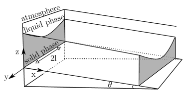
Figure 1: Steady flow on an inclined plane.

In what follows, we will assume that the velocity field is of the form $v(x,y,z)=(u(y,z),0,0)$ for $(x,y,z)\in\{(x,y,z):\,0\leq x,\,-l\leq y\leq l,\,b\leq z\leq h(y)\}$ where $h(y)$ is the interface separating the fluid and the air and $z=b$ is the surface of the inclined plane, the width of which is equal to $2l$. Although the well posedness of similar problems have been studied in more generality in a bounded domain, as it will become clear later, in order to study the interface between the solid and the liquid phase, as we increase the inclination angle, we will need to take $b=-\infty$. By the form of $v$, the incompressibility condition (1.7) is trivially satisfied and equation (1.8) with $\partial_{t}v=0$ becomes

(1.12) $$\hbox{div}\sigma_{\mathrm{dev}}=-f+\nabla p,$$

with $\sigma_{\mathrm{dev}}$ given by (1.10) and

(1.13) $$f=(g_{0}\sin\theta,0,-g_{0}\cos\theta),$$

with $g_{0}$ the gravitational constant. We also assume that $p=p(y,z)$. We calculate

(1.14) $$D(v)=\frac{1}{2}\left(\begin{array}[]{ccc}0&\partial_{y}u&\partial_{z}u\\ \partial_{y}u&0&0\\ \partial_{z}u&0&0\end{array}\right)$$

and $||Du||=\frac{1}{2}|\nabla u|$, with $\nabla u=(\partial_{y}u,\partial_{z}u)$. If we substitute (1.14) in (1.10), equations (1.12) become, for $D(v)\neq 0$ or equivalently $\nabla u\neq 0$,

(1.15) $$[left=\empheqlbrace]\nu\hbox{div}(\nabla u)+\mu_{s}\hbox{div}\left(p\frac{\nabla u}{|\nabla u|}\right) =-g_{0}\sin\theta$$

(1.16) $$0 =\partial_{y}p$$

(1.17) $$0 =g_{0}\cos\theta+\partial_{z}p$$

Where the divergence is taken for the coordinates $(y,z)$. If we integrate equation (1.17) from $z$ to $h(y)$ we get $p(y,z)=(h(y)-z)g_{0}\cos\theta,$ but because of equation (1.16) and because $\theta\in\left[0,\frac{\pi}{2}\right)$ we have $h(y)=h\equiv\text{ constant}$. For simplicity we take $h=0$; then the pressure is given by

(1.18) $$p(y,z)=|z|g_{0}\cos\theta.$$

We are lead to study the following equation

(1.19) $$\begin{cases}\nu\,\hbox{div}(\nabla u)+\mu_{s}g_{0}\cos\theta\,\hbox{div}(|z|q)=-g_{0}\sin\theta&\text{ in }(-l,l)\times(b,0),\\ q\in\partial(|\cdot|)(\nabla u)&\text{ }\end{cases}$$

where $\partial(|\cdot|)$ is the subdifferential of the absolute value. If $(u,q)$ is such that (1.19) holds, with $q=q(y,z)=(q_{1}(y,z),q_{2}(y,z))$, then $|q|\leq 1$ and $q=\frac{\nabla u}{|\nabla u|}$ for $\nabla u\neq 0$ and therefore the stress deviator defined by

(1.20) $$\sigma_{\mathrm{dev}}:=\nu\left(\begin{array}[]{ccc}0&\partial_{y}u&\partial_{z}u\\ \partial_{y}u&0&0\\ \partial_{z}u&0&0\end{array}\right)+\mu_{s}|z|g_{0}\cos\theta\left(\begin{array}[]{ccc}0&q_{1}&q_{2}\\ q_{1}&0&0\\ q_{2}&0&0\end{array}\right)$$

is of the form (1.10) with $v(x,y,z)=(u(y,z),0,0)$ and solves equations (1.12) with $f$ given by (1.13) and $p$ by (1.18).

Boundary conditions

On the surface of the material $z=0$ we assume a no stress condition, i.e. $\sigma\cdot(0,0,1)=0$; since the pressure is zero on the surface near the atmosphere, this condition becomes $\sigma_{\mathrm{dev}}\cdot(0,0,1)=0$. Here we assume that the stress deviator is given by (1.20). Then the stress free condition becomes (since $z=0$)

(1.21) $$\partial_{z}u(y,0)=0.$$

On the lateral boundary $y=\pm 1$ we assume the Dirichlet conditions $u=0$ (no slip), while at the bottom $z=b$, where the material is in contact with the inclined plane, a natural assumption is the friction condition

$$\begin{cases}\sigma n-(\sigma n\cdot n)n=\mu_{C}v&\text{ }\\ v\cdot n=0&\text{ }\end{cases}$$

where $v,\sigma,n,\mu_{C}$ are the velocity, stress, normal to the plane and a friction coefficient respectively. In our case the friction condition reads as follows

(1.22) $$\nu\partial_{z}u+\mu_{s}|b|g_{0}(\cos\theta)q_{2}=\mu_{C}u.$$

Variational formulation

The variational formulation of equation (1.19) with boundary conditions (1.21), (1.22) and the homogeneous Dirichlet conditions on the lateral boundary constitutes in minimizing the energy

(1.23) $$\int_{(-l,l)\times(b,0)}\nu\frac{|\nabla u|^{2}}{2}+\mu_{s}|z|g_{0}\cos\theta|\nabla u|-(g_{0}\sin\theta)u+\mu_{C}\int_{\{z=b\}}\frac{|u|^{2}}{2}$$

with zero lateral boundary conditions, i.e. $u(\pm 1,\cdot)=0$. Since the energy (1.23) is convex and the domain is bounded we can easily get a non-negative minimizer via the direct method.

We are interested in the properties of the minimizer as we increase the inclination angle $\theta$. We call solid and liquid phases the sets $\{(y,z):u(y,z)=0\}$ and $\{(y,z):u(y,z)>0\}$ respectively (often abbreviated as $\{u=0\}$, $\{u>0\}$ resp.), while their common boundary we call a yield curve. We note that usually in the literature the yield curve is defined, for our setting, as the set $\partial\{\nabla u\neq 0\}$, but approximating this set would require different methods and more regularity of the solution.

For $|b|$ small we expect that for a sufficiently large angle $\theta$ all of the material will move due to the gravity, namely there is no solid phase, whereas, if $|b|$ is large enough, even if the inclination is large we expect that there will be a solid phase. In order to study the behaviour and shape of the liquid/solid phases as we increase the inclination angle, we fix $b=-\infty$. However, there is still one more free boundary remaining, the yield curve, i.e. the curve that separates the solid from the liquid phase. Since we study (1.23) in an unbounded domain we drop the friction condition. Let $\tilde{u}$ be a solution of (1.19)-(1.21) with $b=-\infty$, in order to simplify further the equation (1.19) we set

(1.24) $$u(y,z)=\frac{\nu}{\mu_{s}g_{0}\cos\theta}\frac{\tilde{u}\left(ly,lz\right)}{l^{2}},\quad(y,z)\in(-1,1)\times(-\infty,0)$$

we also define

(1.25) $$\lambda:=\frac{\tan\theta}{\mu_{s}},$$

then $\partial|\cdot|(\nabla u(y,z))=\partial|\cdot|(\nabla\tilde{u}(ly,lz))$ and therefore, $u$ given by (1.24) solves the equation (1.1) if and only if $\tilde{u}$ solves (1.19)

As we will see in Theorem 2.3, the minimizer has compact support, therefore, it trivially satisfies the friction condition (1.22) on the solid phase as long as the level of the plane is taken far enough from the support of the minimizer.

We also show that the critical angle for an non-zero minimizer to exist is $\arctan\mu_{s}$, namely for $\theta>\arctan\mu_{s}$ there exists a non-zero solution with a yield curve while for $0\leq\theta\leq\arctan\mu_{s}$ the solution is zero. This angle is known in the literature by experimental study, see for example [16]. The time dependent, one dimensional analogue of our case is studied in [4]; the authors prove that for $\theta>\arctan\mu_{s}$ there is no solution with solid phase while in our case the solution always has a solid phase. The difference of course lies in our two dimensional setting of the problem in which the existence of the walls where the velocity vanishes is crucial, not just for the physical relevance of the problem. Indeed since we study minimizers of (1.3) in an unbounded domain we will often need to apply Poincaré’s inequality, for this reason we need that the projection of the domain in one of the coordinate axes is bounded. In [13] the authors also prove that for $\theta\leq\arctan\mu_{s}$ the flowing material stops moving in finite time.

Review of the literature

For an extensive review of non-Newtonian fluids see [6], also [8] and references therein and [15] for evolutionary problems. The flow of a viscoplastic material with “$\mu(I)-$rheology” is relatively new in the literature, see for example [10]. The inviscid case, i.e. for $\nu=0$ is similar to another scalar model with applications in image processing, the total variation flow, see for example [18] and [2]. Although the total variation bears more similarities with the Bingham case, many of the tools used to study our problem are similar. In fact the total variation is more difficult to study because of the lack of the quadratic term in the energy which leads to lack of regularity of the solution. For the inviscid case our energy (1.3) falls into a wider class, the “total variation functionals” see [3, Hypothesis 4.1]. We refer to [14] for simulations of a regularized Drucker-Prager model with application to granular collapse. Concerning the case of the inclined plane see [11] and [16].

Organization of the paper

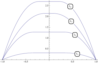
Figure 2: $L_{i},\,i=1,2,3,4$ are the graph of $w$ for $(m,A)=(0.5,0.5),(2,2),(3,0.5),(4,2)$ respectively.

In Section 2 we state our main results, Theorems 2.2 and 2.3. In Subsection 3.1 we study the 1-dimensional analogue of (1.3) which we use in Lemma 3.3; this Lemma is the crucial step in order to prove that the linear term $-\lambda\int_{\Omega}u$ is lower semicontinuous. In Subsection 3.3 we study an approximate problem of the minimizer of (1.3) which helps us to prove certain regularity properties of the solution; we also note that since the minimizer is studied in the half stripe $\Omega$ the regularity holds up to the interface seperating the solid from the liquid phase (the support of the minimizer). Using the approximate minimizer we can also calculate the first variation of (1.3). Finally, in Lemma 4.4 we construct a solution of (1.5) which we use together with the comparison principle from Subsection 4.1, in Subsections 4.3 and 4.4 in order to construct a subsolution and supersolution respectively. The Figures 2-7 as well as the simulations in Table 1 have been made with Mathematica.

2 Main results

We begin with a technical remark.

Remark 2.1.

We have $\mathcal{X}(\Omega)\subset W^{1,1}(\Omega)$, which justifies the choice of the space $\mathcal{X}$ as natural functional space for the functional (1.3). Indeed,

$$\int_{\{|z|\geq 1\}\cap\Omega}|\nabla u|\leq\int_{\{|z|\geq 1\}\cap\Omega}|z||\nabla u|<\infty,$$

from which get that $u\in L^{1}(\Omega)$ by Poincaré’s inequality, see [12, Theorem 12.17]; note also that in our case the proof of Poincaré’s inequality requires only that elements of the space $W^{1,2}(\Omega)$ are zero on the lateral boundary of $\Omega$ (i.e. on $\{\pm 1\}\times(0,\infty)$). In fact, since the width of the walls is $2$ we have $\int_{\Omega}|u|^{p}\leq\frac{2^{p}}{p}\int_{\Omega}|\nabla u|^{p}$ for $p=1,2$.

Let

(2.1) $$\Lambda:=\{q:\,q\in L_{loc}^{2}(\Omega,\mathbb{R}^{2}),\,|q|\leq 1\,\text{ a.e.}\}.$$

Let $\hat{\Omega}=(-1,1)\times\mathbb{R}$, $u\in W^{1,2}_{0L}(\Omega)$, we denote by $\hat{u}\in W^{1,2}_{0L}(\hat{\Omega})$ the reflection of $u$ with respect the $z=0$ axes, i.e.

(2.2) $$\hat{u}(y,z):=\begin{cases}u(y,z)&\text{ if }(y,z)\in\Omega,\\ u(y,-z)&\text{ if }y,z)\in\hat{\Omega}\setminus\Omega.\end{cases}$$

Throughout the paper we will denote the space $\mathcal{X}(\Omega)$ simply by $\mathcal{X}$. Only in Lemma 3.4 we will use the explicit notation, this time for the space $\mathcal{X}(\hat{\Omega})$. The weak formulation of (1.1) is

(2.3) $$\begin{cases}\displaystyle\int_{\Omega}\nu\nabla u\cdot\nabla\varphi+|z|q\cdot\nabla\varphi=\lambda\int_{\Omega}\varphi&\text{for all }\varphi\in\mathcal{X}\\ q\cdot\nabla u=|\nabla u|&\text{a.e.}\end{cases}$$

for some $\lambda\geq 0$, $q\in\Lambda$. We can now state our first main Theorem.

Theorem 2.2.

(Existence and uniqueness of minimizers of (1.3))
Let $\lambda\geq 0$, $E_{\lambda}$ be given by (1.3), then the following hold

1. there exists a unique $0\leq u_{\lambda}\in\mathcal{X}$ such that

   (2.4) $$E_{\lambda}(u_{\lambda})=\inf_{v\in\mathcal{X}}E_{\lambda}(v),$$

   moreover, $u_{\lambda}\equiv 0$ if $\lambda\in[0,1]$ and $u_{\lambda}\not\equiv 0$ if $\lambda\in(1,+\infty)$,

2. there exists $q\in\Lambda$ such that $(u_{\lambda},q)$ solves (2.3),

3. $u_{\lambda}\in C^{0,\alpha}_{\mathrm{loc}}(\Omega)$ for all $\alpha\in(0,1)$, in fact $\hat{u}_{\lambda}\in W^{2,2}_{\mathrm{loc}}(\hat{\Omega})$ and $\partial_{z}u_{\lambda}(y,0)=0$ for $y\in(-1,1)$,

4. if $\lambda>1$, the pair $(u_{\lambda},q)$ obtained in (ii) is unique in the sense that if $(\bar{u}_{\lambda},\bar{q})\in\mathcal{X}\times\Lambda$ is another pair satisfying (2.3) then

   $$u=\bar{u}\text{ in }\Omega,\,\,\text{ and }q=\bar{q},\text{ a.e. in }\{\nabla u\neq 0\}.$$

We set

$$I_{m}:=\inf_{v\in\mathcal{X}}E_{\lambda}(v).$$

Note that by the continuity of the non-negative function $u_{\lambda}$ in Theorem 2.2 we can define the yield curve as the common boundary $\partial\{u_{\lambda}>0\}=\partial\{u_{\lambda}=0\}$. Moreover, the critical value $\lambda=1$ in the previous Theorem is also a critical value of the physical solution by (1.24), (1.25) and it does not depend on the viscosity constant $\nu$ or the width of the walls.

We will give some notations in order to present our second result, the motivation for this notation will become clear in the proofs of the relevant Propositions. Let $\lambda>1$ for $Z\in[\frac{1}{\lambda},\frac{1}{\lambda-1}]$ we define

(2.5) $$f_{\lambda}(Z):=\frac{1}{(\lambda^{2}-1)^{3/2}}\left\{\mathrm{Arcsin}\left[(\lambda^{2}-1)Z-\lambda\right]-\lambda\sqrt{1-\left((\lambda^{2}-1)Z-\lambda\right)^{2}}\right\}.$$

As we will see in the proof of Lemma 4.4, the function $f_{\lambda}$ is strictly increasing in the interval $[\frac{1}{\lambda},\frac{1}{\lambda-1}]$, i.e. $f_{\lambda}(Z_{1})<f_{\lambda}(Z_{2})$ for $Z_{1}<Z_{2}$, with $Z_{1},Z_{2}\in[\frac{1}{\lambda},\frac{1}{\lambda-1}]$; we can therefore define the following function

(2.6) $$\phi_{K(\lambda)}(y):=K(\lambda)f_{\lambda}^{-1}\left(f_{\lambda}\left(\frac{1}{\lambda-1}\right)+\frac{|y|}{K(\lambda)}\right)\quad\text{ }y\in[-1,1],$$

where

(2.7) $$K(\lambda):=\frac{1}{f_{\lambda}\left(\frac{1}{\lambda}\right)-f_{\lambda}\left(\frac{1}{\lambda-1}\right)}.$$

Note that by the monotonicity of $f_{\lambda}$ it is $K(\lambda)<0$. We also define the half cone

(2.8) $$\mathcal{C}_{\lambda}:=\{(y,z)\in\mathbb{R}^{2}:\,0<|y|<z\frac{\lambda}{K(\lambda)}\}$$

and

(2.9) $$\mathrm{Epi}^{\smallsmile}(\lambda):=\{(y,z)\in\Omega:z>\phi_{K(\lambda)}(y)\}.$$

In Lemma 4.4 we show that the sets in (2.9) are increasing in $\lambda$ in the sense that $\mathrm{Epi}^{\smallsmile}(\lambda)\subsetneq\mathrm{Epi}^{\smallsmile}(\bar{\lambda})$ for $\bar{\lambda}>\lambda$, see Figure 3a. For $\lambda_{1}>\lambda$ we set

(2.10) $$\vartheta_{\lambda,\lambda_{1}}:=\frac{\lambda_{1}-\lambda}{2\left(1+\left(\frac{\lambda_{1}}{K(\lambda_{1})}\right)^{2}\right)},$$

(2.11) $$b(\lambda,\lambda_{1}):=1+\sqrt{\frac{\lambda_{1}}{2\vartheta_{\lambda,\lambda_{1}}}},$$

(2.12) $$\Pi(\lambda,\lambda_{1}):=\frac{-K(\lambda_{1})}{\lambda_{1}-1}b(\lambda,\lambda_{1})+\frac{K(\lambda)}{\lambda-1}.$$

and

(2.13) $$\mathrm{Epi}_{\smallsmile}(\lambda_{1}):=\{(y,z)\in\Omega:\,z>b(\lambda,\lambda_{1})\phi_{K(\lambda_{1})}\left(\frac{y}{b(\lambda,\lambda_{1})}\right)\}.$$

In Lemma 4.4 we see that $\displaystyle\min_{|y|\leq 1}\phi_{K(\lambda)}(y)=\phi_{K(\lambda)}(0)=\frac{K(\lambda)}{\lambda-1}$ for all $\lambda>1$, and therefore, the function $\Pi$ in (2.12) is the distance of the projections on the $z-$axes of the epigraphs $\mathrm{Epi}^{\smallsmile}(\lambda)$ and $\Omega\setminus\mathrm{Epi}_{\smallsmile}(\lambda_{1})$. Using (2.7) we calculate

$$\frac{K(\lambda_{1})}{\lambda_{1}-1}=\frac{2(\lambda_{1}+1)\sqrt{\lambda_{1}^{2}-1}}{2\sqrt{\lambda_{1}^{2}-1}+\pi+2\mathrm{Arcsin}\left(\frac{1}{\lambda_{1}}\right)},$$

then $\displaystyle\lim_{\lambda_{1}\rightarrow+\infty}\frac{K(\lambda_{1})}{\lambda_{1}-1}=+\infty$, and similarly one can see that $\displaystyle\lim_{\lambda_{1}\rightarrow+\infty}\frac{K(\lambda_{1})}{\lambda_{1}}=+\infty$; if we combine the above two limits, one can check that for all $\lambda>1$,

(2.14) $$\lim_{\lambda_{1}\rightarrow+\infty}\Pi(\lambda,\lambda_{1})=+\infty.$$

We also have

(2.15) $$\lim_{\lambda_{1}\rightarrow\lambda}\Pi(\lambda,\lambda_{1})=+\infty.$$

If we combine (2.14), (2.15) and the fact that $\Pi$ is continuous and we get that for every fixed $\lambda>1$ the function $\Pi(\lambda,\cdot)$ attains a minimum for some $\lambda^{\star}_{1}>\lambda$. In fact numerical simulations (see Figure 6) suggest the function $\Pi(\lambda,\cdot)$ attains the minimum at a unique $\lambda^{\star}_{1}>\lambda$, but the analytical calculations are too complicated to check.

In the following Theorem we gather the main properties of the solution obtained in Theorem 2.2.

Theorem 2.3.

(Main properties)
Let $\lambda>1$, $\mathcal{X}$ as in (1.4), $(u_{\lambda},q)\in\mathcal{X}\times\Lambda$ be a solution of (2.3). Also let $\lambda_{1}>\lambda$, $\mathrm{Epi}_{\smallsmile}(\lambda_{1})$ be as in (2.13), then then function $u_{\lambda}$ has compact support and it’s support can be estimated as follows

(2.16) $$\mathrm{Epi}^{\smallsmile}(\lambda)\subset\mathrm{supp}\,u_{\lambda}\subset\mathrm{Epi}_{\smallsmile}(\lambda_{1}).$$

Moreover, we can optimize estimate (2.16) by choosing $\lambda_{1}=\lambda^{\star}_{1}$.

Remark 2.4.

(Consequences of Theorem 2.3)

1. In Lemma 4.4 we show that the function $\phi_{K(\lambda)}$ has a strictly negative maximum, therefore estimate (2.16) implies that the yield curve $\partial\{u_{\lambda}>0\}$ never reaches the surface of the atmosphere $\{z=0\}$.

2. Notice that the sets $\mathrm{Epi}^{\smallsmile}(\lambda)$ and $\mathrm{Epi}_{\smallsmile}(\lambda_{1})$ can also estimate the support of the physical solution, by (1.24) and they are independent of the viscosity $\nu$.

3 Existence/Uniqueness

3.1 $1D$-problem

Let $A>0$ and for $w\in W^{1,2}_{0}(-1,1)$ we consider the energy

(3.1) $$\epsilon_{A}(w)=\int_{-1}^{1}\left(\frac{|w^{\prime}(y)|^{2}}{2}+A|w^{\prime}(y)|\right)dy.$$

Using the direct method of calculus of variations it is not difficult to show the following Proposition.

Proposition 3.1.

(Minimizer of $1D$-problem)
Let $A>0$ and $m>0.$ Then there exists a unique function $w$ solving

$$\epsilon_{A}(w)=\inf_{\begin{subarray}{c}\overline{w}\in W^{1,2}_{0}(-1,1)\\ \int_{-1}^{1}\overline{w}=m\end{subarray}}\epsilon_{A}(\overline{w}).$$

We set

(3.2) $$I^{A}_{m}:=\inf_{\begin{subarray}{c}\overline{w}\in W^{1,2}_{0}(-1,1)\\ \int_{-1}^{1}\overline{w}=m\end{subarray}}\epsilon_{A}(\overline{w}).$$

The uniqueness of the minimizer of $\epsilon_{A}$ in the above Proposition follows by the strict convexity of the functional or by using similar arguments as in the proof of Step 1 of Theorem 2.2 (i).

We define the set theoretic sign function as

$$\mathrm{sign}(r):=\begin{cases}\left\{\frac{r}{|r|}\right\}&\text{ if }r\neq 0,\\ (-1,1)&\text{ else.}\end{cases}$$

Proposition 3.2.

(Characterization of the $1D$ minimizer)
Let $A,\,m>0$. If $\lambda_{A}=\lambda_{A,m}$ is the non-negative root of

(3.3) $$2\lambda_{A}^{3}-3\lambda_{A}^{2}(A+m)+A^{3}=0,$$

with $\lambda_{A}>A+m$,

(3.4) $$a=\frac{A}{\lambda_{A}}<1,$$

(3.5) $$w(y)=\begin{cases}A\left(-\frac{y^{2}}{2a}+|y|+\frac{1}{2a}-1\right)&a<|y|<1,\\ \\ A\frac{(a-1)^{2}}{2a}&|y|\leq a.\end{cases}$$

$$q(y)=\begin{cases}-\frac{y}{|y|}&a<|y|<1,\\ \\ -\frac{y}{a}&|y|\leq a,\end{cases}$$

then $(w,q,\lambda_{A})$ solves the equation

(3.6) $$-w^{\prime\prime}(y)-A(q(y))^{\prime}=\lambda_{A},\quad\text{for a.e. }y\in(-1,1),$$

and $\int_{-1}^{1}w=m$. In particular $w$ is the unique minimizer of (3.1) corresponding to the volume constraint $m$.

Proof of Theorem 3.2 
Step 1. The trinomial (3.3)

First we will show that the trinomial (3.3) has a unique non-negative root $\lambda_{A}\geq A+m$. A simple calculation shows that the trinomial (3.3) is increasing in the interval $[A+m,+\infty)$ with values $A^{3}\left(1-\left(1+\frac{m}{A}\right)^{3}\right)\leq 0$ and $+\infty$ for $\lambda_{A}=A+m$ and $\lambda_{A}=+\infty$ respectively, hence there exist a root for $\lambda\geq A+m$.
Step 2. The equation (3.6)

For a.e. $y\in(-1,1)$ we have

(3.7) $$w^{\prime\prime}(y)=\begin{cases}-\frac{A}{a}&a<|y|<1,\\ 0&|y|<a\end{cases}$$

and

(3.8) $$q^{\prime}(y)=\begin{cases}0&a<|y|<1,\\ -\frac{1}{a}&|y|<a.\end{cases}$$

Using (3.7), (3.8) and (3.4) we deduce that $(w,q,\lambda_{A})$ solves (3.6).
Step 3. Volume constraint

It remains to show that $\int_{-1}^{1}w=m$. It is

$$\int_{-1}^{1}w =2\left(\frac{A}{2}(1-a)^{2}+\int_{a}^{1}w\right)$$

$$=2\left(\frac{A}{2}(1-a)^{2}-\frac{A}{2a}\int_{a}^{1}(y-a)^{2}-(1-a)^{2}\,dy\right)$$

$$=\frac{A(1-a)^{2}}{a}-\frac{A}{a}\int_{0}^{1-a}y^{2}\,dy$$

$$=\frac{A}{3a}(1-a)^{2}(2+a),$$

using equation (3.4) and (3.3) we get

(3.9) $$\int_{-1}^{1}w=\frac{A}{3a}(1-a)^{2}(2+a)=\frac{(\lambda_{A}-A)^{2}(2\lambda_{A}+A)}{3\lambda_{A}^{2}}=m.$$

Step 3. Minimizer

It remains to show that $w$ is the minimizer of $\epsilon_{A}$ in $W^{1,2}_{0}(-1,1)$ which corresponds to the constraint $m$. First we notice that $q(x)\in\mathrm{sign}(w^{\prime}(x))=\partial(|\cdot|)(w^{\prime}(x))$ for $x\in(-1,1)$ and the subdifferential is given by (1.2). Let $v\in W^{1,2}_{0}(-1,1)$ with $\int_{-1}^{1}v=m$, it is

$$\epsilon_{A}(v)-\epsilon_{A}(w) \geq\int_{-1}^{1}w^{\prime}(v-w)^{\prime}+Aq(v-w)^{\prime}$$

$$=-\int_{-1}^{1}(w^{\prime\prime}+Aq^{\prime})(v-w)=\lambda_{A}\int_{-1}^{1}(v-w)=0.$$

$\Box$

3.2 A variational problem

The lower semicontinuity of the term $-\int_{\Omega}\lambda u$ in (1.3) under the weak topology of $W^{1,2}$ is not trivial since the integral is not evaluated in a bounded domain. The following Lemma shows that the $L^{1}$-tails of a sequence of functions will converge to zero if the respective values of the functional $E_{\lambda}$ are uniformly bounded.

Lemma 3.3.

(Compensation of the mass)
Let $\{v_{k}\}_{k\in\mathbb{N}}\subset\mathcal{X}$, suppose that there exists a non-negative constant $c$ independent of $k$ such that $E_{\lambda}(v_{k})<c$ for all $k\in\mathbb{N}$, then

(3.10) $$\lim_{l\rightarrow+\infty}\left(\sup_{k}\left(\int_{l}^{+\infty}\int_{-1}^{1}v_{k}(y,-A)\,dydA\right)\right)=0.$$

Proof of Lemma 3.3
  Step 1: An estimate for the minimum of $\epsilon_{A}$

Let $A>0$ and define

(3.11) $$m_{A}=m^{k}_{A}=\int_{-1}^{1}v_{k}(y,-A)\,dy$$

Let $\epsilon_{A}$ be given by (3.1) and $I_{m_{A}}^{A}$ be the minimum of $\epsilon_{A}$ corresponding to the constraint $m_{A}$. Then for $\lambda_{A}$ the root of the trinomial in (3.3), it is

$$m_{A}=\frac{(\lambda_{A}-A)^{2}(2\lambda_{A}+A)}{3\lambda_{A}^{2}}.$$

Using (3.5) we calculate

(3.12) $$I_{m_{A}}^{A}=\frac{A^{2}}{a}\left(\frac{2}{3}\frac{(1-a)^{3}}{a}+(1-a)^{2}\right)=\frac{(\lambda_{A}-A)^{2}(2\lambda_{A}+A)}{3\lambda_{A}}=m_{A}\lambda_{A}.$$

By Step 1 of the proof of Proposition 3.2 we have $\lambda_{A}\geq A+m_{A}$ hence equation (3.12) becomes

(3.13) $$I_{m_{A}}^{A}\geq m_{A}(A+m_{A})\geq Am_{A}.$$

Step 2: The tails of $v_{k}$ converge uniformly to $0$

We argue by contradiction, suppose that

$$\sup_{k}\left(\int_{l}^{+\infty}m^{k}_{A}\,dA\right)\nrightarrow 0\text{ as }l\rightarrow+\infty$$

then, there are $\varepsilon>0$ and a sequence $l_{j}\rightarrow+\infty$ as $j\rightarrow+\infty$ such that

(3.14) $$\sup_{k}\left(\int_{l_{j}}^{+\infty}m^{k}_{A}\,dA\right)\geq\varepsilon$$

By Fubini’s Lemma we have for $l_{j}>\lambda$

(3.15) $$E_{\lambda}(v_{k}) =\int_{0}^{+\infty}\int_{-1}^{1}\frac{|\nabla v_{k}|^{2}}{2}+A|\nabla v_{k}|-\lambda v_{k}\,\mathrm{d}y\mathrm{d}A$$

$$\geq\int_{0}^{+\infty}\int_{-1}^{1}\frac{|\partial_{y}v_{k}|^{2}}{2}+A|\partial_{y}v_{k}|-\lambda v_{k}\,\mathrm{d}y\mathrm{d}A$$

$$\geq\int_{l_{j}}^{+\infty}I_{m^{k}_{A}}^{A}-\lambda m_{A}^{k}\,dA\geq\int_{l_{j}}^{+\infty}m^{k}_{A}(l_{j}-\lambda)\,dA,$$

where in the last inequality we used (3.11), (3.2) and (3.13). Taking the supremum over $k\in\mathbb{N}$ we get, using (3.14)

$$c\geq\sup_{k}E_{\lambda}(v_{k})\geq\sup_{k}\left(\int_{l_{j}}^{+\infty}m^{k}_{A}(l_{j}-\lambda)\,dA\right)\geq(l_{j}-\lambda)\varepsilon\rightarrow+\infty\quad\text{ as }l_{j}\rightarrow+\infty,$$

a contradiction.
$\Box$

We have the following Lemma.

Lemma 3.4.

(Approximation by smooth functions)
Let $v\in\mathcal{X}(\hat{\Omega})$. Then, there is a sequence $v_{A}\in W^{1,2}_{0}(\hat{\Omega})$ such that

(3.16) $$v_{A}\rightarrow v\text{ in }W^{1,2}(\hat{\Omega})\cap L^{1}(\hat{\Omega}),$$

and

(3.17) $$\lim_{A\rightarrow+\infty}\int_{\hat{\Omega}}|z||\nabla v_{A}-\nabla v|=0.$$

Proof of Lemma 3.4
  First we note that $v\in L^{1}(\hat{\Omega})$ by Remark 2.1. Let $A>1$ we define the cut off functions $\eta_{A}\in W^{1,\infty}_{0}(\mathbb{R})$ by

$$\eta_{A}(z):=\begin{cases}1&\text{ if }|z|\leq A,\\ 1-\frac{1}{A}(|z|-A)&\text{ if }A\leq|z|\leq 2A,\\ 0&\text{ if }2A\leq|z|.\end{cases}$$

Then

(3.18) $$|\eta^{\prime}_{A}(z)|\leq\frac{2}{|z|}\text{ a.e. }$$

The functions $v_{A}(y,z):=\eta_{A}(z)v(y,z)$ belong to $W^{1,2}(\hat{\Omega})$, they have compact support in $\hat{\Omega}_{A}=(-1,1)\times(-2A,2A)$ and zero trace on $\partial\hat{\Omega}_{A}$. Since the boundary of each $\hat{\Omega}_{A}$ is Lipschitz and bounded we have by [12, Theorem 15.29] that $v_{A}\in W^{1,2}_{0}(\hat{\Omega}_{A})$. It is not difficult to see that $v_{A}\rightarrow v$ in $W^{1,2}(\hat{\Omega})$, we will show that $\displaystyle\lim_{A\rightarrow+\infty}|z||\nabla v_{A}-\nabla v|=0$.
We have

$$\int_{\hat{\Omega}}|z||\nabla v_{A}-\nabla v| \leq\int_{\hat{\Omega}}|z|(|\eta^{\prime}_{A}v|+|\eta_{A}-1||\nabla v|)$$

$$\leq\int_{\hat{\Omega}\cap\{A<|z|<2A\}}2|v|+\int_{\hat{\Omega}\cap\{A<|z|\}}|z||\nabla v|$$

then, using (3.18) and the fact that $|z||\nabla v|,|v|\in L^{1}(\hat{\Omega})$ the right hand side of the above estimate converges to zero as $A\rightarrow+\infty$.
The convergence in $L^{1}(\hat{\Omega})$ in (3.16) follows by Remark 2.1. $\Box$

For two sets $U,U^{\prime}\subset\mathbb{R}^{2}$, by $U\subset\subset U^{\prime}$ we mean that $U$ is relatively compact in $U^{\prime}$, i.e. $\overline{U}\subset U^{\prime}$ and $\overline{U}$ is compact. Also for a function $u(y,z)$ we define the positive part $u^{+}(y,z)=\max\{u(y,z),0\}$.

Proof of Theorem 2.2 (i)
  Step 1. Boundedness of $E_{\lambda}$ from below

We focus in the cases $\lambda>0$ since for $\lambda=0$ the minimizer of $E_{\lambda}$ is trivially the zero function. We fix $\lambda>0$, let $u\in\mathcal{X}$, using Poincaré’s inequality in $\Omega$ (Remark 2.1) we get

$$E_{\lambda}(u) =\int_{\Omega}\frac{|\nabla u|^{2}}{2}+|z||\nabla u|-\lambda\int_{\Omega}u$$

$$\geq\int_{\Omega}\frac{|\nabla u|^{2}}{2}+(|z|-2\lambda)|\nabla u|.$$

We split the last integral in the domains $\{|z|\geq 2\lambda\}\cap\Omega$ and $\{|z|\leq 2\lambda\}\cap\Omega$ and get

$$E_{\lambda}(u) \geq\int_{\{|z|\leq 2\lambda\}\cap\Omega}\frac{|\nabla u|^{2}}{2}-2\lambda|\nabla u|$$

$$\geq\int_{\{|z|\leq 2\lambda\}\cap\Omega}-2\lambda^{2}>-\infty.$$

Step 2. Minimizing sequence

Let $u_{k}\in\mathcal{X}$ with $\displaystyle\lim_{k\rightarrow+\infty}E_{\lambda}(u_{k})=\inf_{v\in\mathcal{X}}E_{\lambda}(v)$. We will denote by $c$ a generic positive constant which does not depend on the parameter $k$. There is a positive constant $c$ such that $\displaystyle\sup_{k\in\mathbb{N}}E_{\lambda}(u_{k})\leq c$, then as in Step 1 we use Poincare’s inequality to get

$$c \geq\int_{\{|z|\leq 2\lambda\}\cap\Omega}\frac{|\nabla u_{k}|^{2}}{2}+(|z|-2\lambda)|\nabla u_{k}|+\int_{\{|z|\geq 2\lambda\}\cap\Omega}\frac{|\nabla u_{k}|^{2}}{2}$$

$$\geq\int_{\{|z|\leq 2\lambda\}\cap\Omega}\frac{|\nabla u_{k}|^{2}}{2}-\frac{|\nabla u_{k}|^{2}}{4}-(|z|-2\lambda)^{2}+\int_{\{|z|\geq 2\lambda\}\cap\Omega}\frac{|\nabla u_{k}|^{2}}{2},$$

where in the second inequality we used Young’s inequality$\left(|a||b|\leq\frac{b^{2}}{4}+a^{2}\right)$. Is is easy now to see that

(3.19) $$\int_{\Omega}|\nabla u_{k}|^{2}\leq c.$$

Then by Poincare’s inequality and compactness there is $u\in W^{1,2}_{0L}(\Omega)$ such that $u_{k}\rightharpoonup u$ as $k\rightarrow+\infty$.

Using similar arguments we get $c\geq\int_{\Omega}(|z|-2\lambda)|\nabla u_{k}|$, or if we split the integral in the domains $\{|z|\geq 4\lambda\}\cap\Omega=\{|z|-2\lambda\geq|z|/2\}\cap\Omega$ and $\{|z|\leq 4\lambda\}\cap\Omega$ we get

(3.20) $$\frac{1}{2}\int_{\{|z|-2\lambda\geq|z|/2\}\cap\Omega}|z||\nabla u_{k}|\leq\int_{\{|z|\geq 4\lambda\}\cap\Omega}(|z|-2\lambda)|\nabla u_{k}|\leq c-\int_{\{|z|\leq 2\lambda\}\cap\Omega}(|z|-2\lambda)|\nabla u_{k}|,$$

since $\int_{\{2\lambda\leq|z|\leq 4\lambda\}\cap\Omega}(|z|-2\lambda)|\nabla u_{k}|\geq 0$. We can now bound the right hand side of (3.20) using Hölders inequality and (3.19) and get eventually that $\int_{\{|z|\geq 4\lambda\}\cap\Omega}|z||\nabla u_{k}|\leq c$. Using Hölders inequality and (3.19), one can also bound the quantity $\int_{\{|z|\leq 4\lambda\}\cap\Omega}|z||\nabla u_{k}|$ uniformly in $k$, we can therefore conclude that

(3.21) $$\int_{\Omega}|z||\nabla u_{k}|\leq c,$$

where again $c$ is a positive constant independent of $k$.
Step 3. Lower semicontinuity

We will show that

(3.22) $$\int_{\Omega}\frac{|\nabla u|^{2}}{2}+|z||\nabla u|\leq\liminf_{k\rightarrow+\infty}\int_{\Omega}\frac{|\nabla u_{k}|^{2}}{2}+|z||\nabla u_{k}|,$$

and

(3.23) $$-\lambda\int_{\Omega}u\leq\liminf_{k\rightarrow+\infty}\left(-\lambda\int_{\Omega}u_{k}\right).$$

Equations (3.19), (3.21) and (3.22) imply that $u\in\mathcal{X}$ and then $u\in L^{1}(\Omega)$ by Remark 2.1. Whereas, equations (3.22) and (3.23) together imply that $E_{\lambda}(u)\leq\displaystyle\liminf_{k\rightarrow+\infty}E_{\lambda}(u_{k})$, which shows that $u$ is a minimizer of $E_{\lambda}$ in $\mathcal{X}$. Since the integrand in (3.22) is non-negative convex in the gradient variable and measurable in the $z$ variable, the inequality (3.22) follows from [9, Chapter I, Theorem 2.5].

For $l>0$ fixed we have

(3.24) $$\int_{\Omega}u_{k} =\int_{l}^{+\infty}\int_{-1}^{1}u_{k}(y,-A)\,dydA+\int_{0}^{l}\int_{-1}^{1}u_{k}(y,-A)\,dydA$$

(3.25) $$\leq\sup_{k}\left(\int_{l}^{+\infty}\int_{-1}^{1}u_{k}(y,-A)\,dydA\right)+\int_{0}^{l}\int_{-1}^{1}u_{k}(y,-A)\,dydA.$$

Since $E_{\lambda}(u_{k})$ is uniformly bounded we can apply Lemma 3.3 and get that (3.10) holds for the sequence $u_{k}$. Using (3.10) and the fact that $u\in L^{1}(\Omega)$, we can take the $\limsup$ in (3.24), as $k\rightarrow+\infty$ and then $l\rightarrow+\infty$ and get $\displaystyle\limsup_{k\rightarrow+\infty}\int_{\Omega}u_{k}\leq\int_{\Omega}u$ or else (3.23), which completes the proof of the lower semi-continuity of $E_{\lambda}$ and hence the existence of a minimizer $u\in\mathcal{X}$.
Step 4. Uniqueness

Let $u,\tilde{u}\in\mathcal{X}$ be two minimizers, then using similar arguments as in [6, Section 3.5.4, p.36] one can show that

(3.26) $$\int_{\Omega}\nabla u\cdot(\nabla\tilde{u}-\nabla u)+\int_{\Omega}|z||\nabla\tilde{u}|-\int_{\Omega}|z||\nabla u|\geq\lambda\int_{\Omega}\tilde{u}-u,$$

(3.27) $$\int_{\Omega}\nabla\tilde{u}\cdot(\nabla u-\nabla\tilde{u})+\int_{\Omega}|z||\nabla u|-\int_{\Omega}|z||\nabla\tilde{u}|\geq\lambda\int_{\Omega}u-\tilde{u}.$$

If we add equations (3.26) and (3.27) we get

$$\int_{\Omega}|\nabla u-\nabla\tilde{u}|^{2}\leq 0,$$

hence $u=\tilde{u}$ in $\Omega$ since they also have the same lateral boundary conditions.
Step 5. Non-negative minimizer

We have by [19, Corollary 2.1.8, page 47] that $\nabla u^{+}=(\nabla u)\cdot\chi_{\{u>0\}}$, where by $\chi_{\{u>0\}}$ we denote the characteristic function of the set $\{(y,z):u(y,z)>0\}$. Since also $-\lambda\int_{\Omega}u^{+}\leq-\lambda\int_{\Omega}u$ we have $E_{\lambda}(u^{+})\leq E_{\lambda}(u)$, hence $u=u^{+}$ by the uniqueness of minimizers.
Step 6. $\lambda\in[0,1]$

Our goal is to show that

(3.28) $$E_{\lambda}(u)\geq 0,\quad\text{ for all }u\in\mathcal{X},$$

then because $0\in\mathcal{X}$ and $E_{\lambda}(0)=0$ we get that the unique minimizer of $E_{\lambda}$ is the zero function. In view of Lemma 3.4, it is enough to prove (3.28) for functions $u$ with $\hat{u}\in W^{1,2}_{0}(\hat{\Omega})$. Let $u$ be such a function, then as in Step 5 we have

(3.29) $$E_{\lambda}(u^{+})\leq E_{\lambda}(u).$$

Suppose that the compact support of $\hat{u}^{+}$ is contained in $[-1,1]\times(-A,A)$ where $A$ is large enough, then we have

$$\int_{\Omega}|z||\nabla u^{+}| \geq\int_{-1}^{1}\int_{0}^{A}|z|\left|\frac{\partial u^{+}}{\partial z}\right|\,dzdy$$

$$\geq\left|\int_{-1}^{1}\int_{0}^{A}z\frac{\partial u^{+}}{\partial z}\,dzdy\right|$$

$$=\int_{\Omega}u^{+}$$

in the last equality we used integration by parts. This estimate together with (3.29) and the fact that $\lambda\leq 1$ gives

$$E_{\lambda}(u)\geq E_{\lambda}(u^{+})\geq(1-\lambda)\int_{\Omega}u^{+}\geq 0.$$

Step 7. $\lambda\in(1,+\infty)$

Our goal is to prove that there is $u\in\mathcal{X}$ with $E_{\lambda}(u)<0$. Let $\varphi\in C^{\infty}(-1,1)$, $\varphi\geq 0$ with $\varphi(-1)=0=\varphi(1)$ and $\int_{-1}^{1}\varphi=1$ (for example $\varphi(y)=\frac{3}{4}(1-y^{2})$). We define

$$u(y,z):=k^{-3}e^{kz}\varphi(y)$$

where $k>0$ is large enough, to be chosen later. It is $u\in\mathcal{X}$ and

(3.30) $$\int_{\Omega}\frac{|\nabla u|^{2}}{2} =\frac{1}{2}\int_{-1}^{1}\left[k^{-2}(\varphi^{\prime}(y))^{2}+\varphi^{2}(y)\right]dy\int_{-\infty}^{0}(k^{-2}e^{kz})^{2}\,dz$$

$$=\frac{A_{k}}{4}k^{-5}$$

where we set $A_{k}=\int_{-1}^{1}\left[k^{-2}(\varphi^{\prime}(y))^{2}+\varphi^{2}(y)\right]\,dy$. Also

(3.31) $$\int_{\Omega}|z||\nabla u| =\int_{-1}^{1}\sqrt{k^{-2}(\varphi^{\prime}(y))^{2}+\varphi^{2}(y)}\,dy\int_{-\infty}^{0}|z|k^{-2}e^{kz}\,dz$$

$$=B_{k}\int_{-\infty}^{0}|z|k^{-2}e^{kz}\,dz$$

where $B_{k}=\int_{-1}^{1}\sqrt{k^{-2}(\varphi^{\prime}(y))^{2}+\varphi^{2}(y)}\,dy$. If we integrate by parts the second product component of the right hand side of (3.31) we get

$$\int_{-\infty}^{0}|z|k^{-2}e^{kz}\,dz=\int_{-\infty}^{0}k^{-3}e^{kz}=\int_{-\infty}^{0}k^{-3}e^{kz}\int_{-1}^{1}\varphi=\int_{\Omega}u,$$

then (3.31) becomes

(3.32) $$\int_{\Omega}|z||\nabla u|=B_{k}\int_{\Omega}u.$$

We also have $\int_{\Omega}u=k^{-4}$, then we can write $E_{\lambda}(u)$ using (3.30) and (3.32) as

(3.33) $$E_{\lambda}(u)=\frac{A_{k}}{4}k^{-5}+(B_{k}-\lambda)k^{-4}.$$

Next we note that $B_{k}\geq 1$, is decreasing in $k$ (and so is $A_{k}$) and $B_{k}\rightarrow 1$ as $k\rightarrow+\infty$. Since $\lambda>1$ we can find $k_{0}$ large enough such that $B_{k_{0}}<\lambda$, then (3.33) becomes

$$E_{\lambda}(u)\leq\frac{A_{k_{0}}}{4}k^{-5}+(B_{k_{0}}-\lambda)k^{-4},$$

for all $k\geq k_{0}$. We can now conclude if we choose $k\geq k_{0}$ large enough, since the function $k^{-5}$ decreases faster than $k^{-4}$, for example $k>\max\{k_{0},\frac{A_{k_{0}}}{4(\lambda-B_{k_{0}})}\}$. $\Box$

3.3 The $\varepsilon$-approximation

Let $\lambda>0$, $u_{\lambda}$ be the minimizer of $E_{\lambda}$ given by Theorem 2.2 (i). For $A>0$ we define $\hat{\Omega}_{A}=\{(y,z)\in\hat{\Omega}:\,|z|\leq A\}$, $\Omega_{A}=\Omega\cap\hat{\Omega}_{A}$ and

$$\mathcal{H}_{A}=\{v\in W^{1,2}(\Omega_{A}),\,v=u_{\lambda},\text{ on }\partial\Omega_{A}\setminus\{z=0\}\},$$

We are interested in approximate minimizers of (1.3), for this we study the minimizers in $\mathcal{H}_{A}$ of the approximate functional

(3.34) $$E^{A}_{\varepsilon,\lambda}(u)=\int_{\Omega_{A}}\frac{|\nabla u|^{2}}{2}+|z|\sqrt{\varepsilon^{2}+|\nabla u|^{2}}-\lambda u,$$

where $\varepsilon>0$.
Since we have mixed boundary conditions, an easy way to describe the space of test functions for the weak formulation of the first variation of (3.34) is to use reflection in the domain $\hat{\Omega}_{A}$. We will simply write $\hat{\phi}\in W^{1,2}_{0}({\hat{\Omega}_{A}})$ for the test functions. We have the following Proposition.

Proposition 3.5.

($W^{2,2}_{\mathrm{loc}}$ regularity of approximate problem)
Let $A,\varepsilon,\lambda>0$, then there exists a unique minimizer $u_{\varepsilon,A}\in\mathcal{H}_{A}$ of $E^{A}_{\varepsilon,\lambda}$. Moreover, $\hat{u}_{\varepsilon,A}\in W^{2,2}_{\mathrm{loc}}(\hat{\Omega}_{A})$ and the following equation holds

(3.35) $$\int_{\Omega_{A}}\nabla u_{\varepsilon,A}\cdot\nabla\varphi+|z|\frac{\nabla u_{\varepsilon,A}\cdot\nabla\varphi}{\sqrt{\varepsilon^{2}+|\nabla u_{\varepsilon,A}|^{2}}}=\lambda\int_{\Omega_{A}}\varphi,\quad\text{ for all }\hat{\varphi}\in W^{1,2}_{0}(\Omega_{A}),$$

and $\partial_{z}u_{\varepsilon,A}(y,0)=0$ for $y\in(-1,1)$.

The existence of a minimizer is a consequence of the direct method in the bounded domain $\Omega_{A}$, while the regularity results are standard. We give a sketch of the Proof of Proposition 3.5 in Appendix A.

Proof of Theorem 2.2 (ii)-(iv)
  Step 1. Solutions of E-L equation are minimizers of (1.3)

First we will show that for any pair $(u,q)\in\mathcal{X}\times\Lambda$ that satisfies equation (2.3), $u$ is a minimizer of $E_{\lambda}$. Let $v\in\mathcal{X}$, using (2.3) and the fact that $|q|\leq 1$ it is easy to check that $q\in\partial|\cdot|(\nabla u)$ in $\Omega$. By the definition of the subdifferential we have

(3.36) $$E_{\lambda}(v)-E_{\lambda}(u)\geq\int_{\Omega}\nabla u\cdot\nabla(v-u)+|z|q\cdot\nabla(v-u)-\lambda\int_{\Omega}(v-u)=0,$$

where we used (2.3) with test function $\varphi=v-u\in\mathcal{X}$.
Step 2. Approximating solutions

As usual we will focus in the case $\lambda>0$. Let $u=u_{\lambda}$ be the minimizer of $E_{\lambda}$ given by Theorem 2.2 (i). For $\varepsilon>0$ let $u_{\varepsilon,A}$ be the minimizer of $E^{A}_{\varepsilon,\lambda}$ given by Proposition 3.5, then for all $A>0$ we will show that $u_{\varepsilon,A}\rightarrow u$ strongly as $\varepsilon\rightarrow 0$, in $W^{1,2}(\Omega_{A})$ up to a subsequence. Extending $u_{\varepsilon,A}$ by $u_{\lambda}$ outside $\Omega_{A}$, we can write the following variational inequalities as in the Step 1 of the proof of Theorem 2.2 (i)

(3.37) $$\int_{\Omega_{A}}\nabla u\cdot(\nabla u_{\varepsilon,A}-\nabla u)+\int_{\Omega_{A}}|z||\nabla u_{\varepsilon,A}|-\int_{\Omega_{A}}|z||\nabla u|\geq\lambda\int_{\Omega_{A}}u_{\varepsilon,A}-u$$

and

(3.38) $$\int_{\Omega_{A}}\nabla u_{\varepsilon,A}\cdot(\nabla u-\nabla u_{\varepsilon,A})+\int_{\Omega_{A}}|z|\sqrt{\varepsilon^{2}+|\nabla u|^{2}}-\int_{\Omega_{A}}|z|\sqrt{\varepsilon^{2}+|\nabla u_{\varepsilon,A}|^{2}}\geq\lambda\int_{\Omega_{A}}u-u_{\varepsilon,A}.$$

Adding inequalities (3.37) and (3.38), we get

$$\int_{\Omega_{A}}|\nabla u_{\varepsilon,A}-\nabla u|^{2} \leq\int_{\Omega_{A}}|z|(|\nabla u_{\varepsilon,A}|-\sqrt{\varepsilon^{2}+|\nabla u_{\varepsilon,A}|^{2}})+|z|(\sqrt{\varepsilon^{2}+|\nabla u|^{2}}-|\nabla u|)$$

$$\leq\int_{\Omega_{A}}|z|(\sqrt{\varepsilon^{2}+|\nabla u|^{2}}-|\nabla u|)$$

$$=\int_{\Omega_{A}}|z|\frac{\varepsilon^{2}}{\sqrt{\varepsilon^{2}+|\nabla u|^{2}}+|\nabla u|}\leq A|\Omega_{A}|\varepsilon,$$

Then using also Poincare’s inequality we get for all $A>0$ and up to a subsequence

(3.39) $$\nabla u_{\varepsilon,A}\rightarrow\nabla u,\,u_{\varepsilon,A}\rightarrow u\text{ a.e. in }\Omega_{A}\text{ as }\varepsilon\rightarrow 0.$$

Step 3. The function $q$

For $q_{\varepsilon,A}=\frac{\nabla u_{\varepsilon,A}}{\sqrt{\varepsilon^{2}+|\nabla u_{\varepsilon,A}|^{2}}}$, we have $q_{\varepsilon,A}\cdot\nabla u_{\varepsilon,A}\leq|\nabla u_{\varepsilon,A}|$, then using (3.39) it is not difficult to see that

(3.40) $$q_{\varepsilon,A}\cdot\nabla u_{\varepsilon,A}\rightarrow|\nabla u|\text{ a.e. in }\Omega_{A}\text{ as }\varepsilon\rightarrow 0.$$

Since $q_{\varepsilon,A}\in L_{\mathrm{loc}}^{2}(\Omega_{A},\mathbb{R}^{2})$ with $|q_{\varepsilon,A}|\leq 1$, there exists $q_{A}\in L_{\mathrm{loc}}^{2}(\Omega_{A},\mathbb{R}^{2})$ with $|q_{A}|\leq 1$ and such that $q_{\varepsilon,A}$ converges weakly to $q_{A}$ in $L^{2}(U,\mathbb{R}^{2})$, as $\varepsilon\rightarrow 0$, for every $U\subset\subset\Omega_{A}$. Then using also (3.39) we have $\displaystyle\lim_{\varepsilon\rightarrow 0}\int_{U}q_{\varepsilon,A}\cdot\nabla u_{\varepsilon,A}=\int_{U}q_{A}\cdot\nabla u$ for all $U\subset\subset\Omega_{A}$ and by (3.40) we get that $q_{A}\cdot\nabla u=|\nabla u|$ a.e. in $\Omega_{A}$. Extending $q_{A}$ by zero outside $\Omega_{A}$ we may wright $q_{A}\in L^{2}_{\mathrm{loc}}(\Omega,\mathbb{R}^{2})$ and as before we can find $q\in L^{2}_{\mathrm{loc}}(\Omega,\mathbb{R}^{2})$, with $|q|\leq 1$ and such that $q_{A}$ converges weakly to $q$ in $L^{2}(U,\mathbb{R}^{2})$, as $A\rightarrow+\infty$, for every $U\subset\subset\Omega_{A}$, and hence $q\cdot\nabla u=|\nabla u|$ a.e.
Step 4. Passing to the limit $\varepsilon\rightarrow 0,A\rightarrow+\infty$

Let $\varphi$ with $\hat{\varphi}\in W^{1,2}_{0}(\hat{\Omega})$, then equation (3.35) with $A$ large enough holds for this test function and since $q_{\varepsilon,A}$ is bounded we can pass to the limit as $\varepsilon\rightarrow 0$ and get

$$\int_{\Omega}\nabla u\cdot\nabla\varphi+|z|q_{A}\cdot\nabla\varphi=\lambda\int_{\Omega}\varphi.$$

We can now pass to the limit as $A\rightarrow+\infty$ and using also Lemma 3.4 we get (2.3).
Step 5. Uniqueness

Let $(u,q)$, $(\bar{u},\bar{q})$ be two solutions of (2.3) then by Step 1 we have $u=\bar{u}$, since minimizers of (1.3) in $\mathcal{X}$ are unique by Theorem 2.2 (i). Then in the set $\{\nabla u\neq 0\}$ the vectors $q,\bar{q}$ are parallel to $\nabla u$ and so is $q-\bar{q}$, but since $(q-\bar{q})\cdot\nabla u=0$ by (2.3) we have $q=\bar{q}$ a.e. in $\{\nabla u\neq 0\}$.
Step 6. Neumann condition

We denote by $\partial_{x_{i}}$, $i=1,2$ respectively the derivatives $\partial_{y},\,\partial_{z}$. Let $i,j\in\{1,2\}$, $\hat{U}\subset\subset\hat{\Omega}_{A}$, by Proposition 3.5 we have that $\hat{u}_{\varepsilon,A}\in W^{2,2}_{\mathrm{loc}}(\hat{U})$, by Lemma A.1 the second derivatives of $\hat{u}_{\varepsilon,A}$ are uniformly bounded in $L^{2}(\hat{U})$, hence for $\varphi\in W^{1,2}_{0}(\hat{U})$ we have (up to a subsequence)

$$\int_{\hat{U}}\partial_{x_{i}}\hat{u}\partial_{x_{j}}\varphi=\lim_{\varepsilon\rightarrow 0}\int_{\hat{U}}\partial_{x_{i}}\hat{u}_{\varepsilon,A}\partial_{x_{j}}\varphi=-\lim_{\varepsilon\rightarrow 0}\int_{\hat{U}}\partial_{x_{j}}\partial_{x_{i}}\hat{u}_{\varepsilon,A}\varphi=-\int_{\hat{U}}g\varphi,$$

for some function $g\in L^{2}(\hat{U})$. We have proved that $\hat{u}\in W^{2,2}_{\mathrm{loc}}(\hat{\Omega})$, then applying a Sobolev embedding Theorem ([7, Section 5.6.3]) we get that $\hat{u}\in C^{0,\alpha}_{\mathrm{loc}}(\hat{\Omega})$ for all $\alpha\in(0,1)$. As in the proof of Proposition 3.5 we can now define the trace of the derivative of $u$ on $\{z=0\}$ and $\partial_{z}u(y,0)=0$ for $y\in(-1,1)$. $\Box$

4 Properties of the solution

4.1 Comparison Principle

In view of Theorem 2.2 (i) we will assume that $\lambda>1$ for the rest of the paper.

Definition 4.1.

Sub/supersolution
Let $u\in\mathcal{X}$ be non-negative and $q\in\Lambda$, $\Lambda$ as in (2.1), we call the pair $(u,q)$ a subsolution (resp. a supersolution) of the equation (2.3) if

(4.1) $$\begin{cases}\int_{\Omega}\nabla u\cdot\nabla\varphi+|z|q\cdot\nabla\varphi\leq\lambda\int_{\Omega}\varphi\,\,(\text{resp.}\geq\lambda\int_{\Omega}\varphi)&\text{for all }\varphi\in\mathcal{X},\varphi\geq 0,\\ q\cdot\nabla u=|\nabla u|&\text{a.e. in }\Omega.\end{cases}$$

Proposition 4.2.

Comparison principle
Let $u,v\in\mathcal{X}$, $q_{u},q_{v}\in\Lambda$ with $(u,q_{u}),(v,q_{v})$ a subsolution and a supersolution respectively of (2.3), with $0=u\leq v$ on $\{-1,1\}\times(-\infty,0)$ in the sense of traces, then

$$u\leq v,\quad\text{ in }\Omega.$$

Proof of Proposition 4.2 
Let $\varphi=(u-v)_{+}$, then $\varphi\in\mathcal{X}$. If we write the inequalities (4.1) for $u,v$ with this test function and subtract the one from the other we get

$$\int_{\Omega}\nabla(u-v)\cdot\nabla(u-v)_{+}+|z|(q_{u}-q_{v})\cdot\nabla(u-v)_{+}\leq 0,$$

or if we use [19, Corollary 2.1.8, page 47] we can write it as

(4.2) $$\int_{\Omega}|\nabla(u-v)|^{2}\chi_{\{u-v\geq 0\}}\leq-\int_{\Omega}|z|\left[(q_{u}-q_{v})\cdot\nabla(u-v)\right]\chi_{\{u-v\geq 0\}}.$$

Next we calculate, using the properties of $q_{u},q_{v}$ in Definition 4.1

$$(q_{u}-q_{v})\cdot(\nabla u-\nabla v) =|\nabla u|-q_{u}\cdot\nabla v-q_{v}\cdot\nabla u+|\nabla v|$$

$$\geq|\nabla u|-|\nabla u|+|\nabla v|-|\nabla v|=0,\,\text{ a.e.}$$

then (4.2) implies

$$\nabla(u-v)=0,\quad\text{ a.e. in }\{u-v\geq 0\}$$

or $\nabla(u-v)_{+}=0$ almost everywhere. Using the boundary conditions we can conclude that $(u-v)_{+}=0$ and hence $u\leq v$ a.e. in $\Omega$. $\Box$

Remark 4.3.

(Monotonicity in $\lambda$)
For $u_{\lambda}$ the minimizer of $E_{\lambda}$ in $\mathcal{X}$ and $m(\lambda)=\int_{\Omega}u_{\lambda}$ the volume rate, using the comparison principle from Proposition 4.2 it is not difficult to see that $m(\lambda)$ is increasing in $\lambda$. Unfortunately, the physical volume rate is given, using the rescaling (1.24), by $m_{0}=(l^{2}\mu_{s}g_{0}\cos\theta)m$, which does not allow us to directly study the monotonicity with respect the inclination angle $\theta$ ($\cos\theta$ is decreasing for $\theta\in[0,\pi/2)$ and $\lambda(\theta)$ is increasing by (1.25)).

4.2 Some explicit profiles

As we explained in the introduction, we study the first variation of the functional (1.6), i.e.

(4.3) $$\frac{\phi\phi^{\prime\prime}}{(1+|\phi^{\prime}|^{2})^{3/2}}-\frac{1}{\sqrt{1+|\phi^{\prime}|^{2}}}+\lambda=0,\quad y\in(-1,1).$$

Lemma 4.4.

(An explicit solution of 4.3)
Let $\lambda>1$, $K(\lambda)$ be given by (2.7) and $\phi_{K(\lambda)}$ defined in (2.6). Then the function $\phi_{K(\lambda)}\in C^{\infty}(-1,1)\cap C([-1,1])$ is non-positive and the following properties hold

(4.4) $$\lim_{y\rightarrow-1}\phi_{K(\lambda)}^{\prime}(y)=-\infty,\,\displaystyle\lim_{y\rightarrow 1}\phi_{K(\lambda)}^{\prime}(y)=+\infty.$$

Moreover the function $\phi_{K(\lambda)}$ is convex with minimum $\phi_{K(\lambda)}(0)=\frac{K(\lambda)}{\lambda-1}$ and maximum $\phi_{K(\lambda)}(\pm 1)=\frac{K(\lambda)}{\lambda}$ and if $\bar{\lambda}>\lambda$ then $\phi_{K(\bar{\lambda})}(y)<\phi_{K(\lambda)}(y)$, for $y\in[-1,1]$.

Proof of Lemma 4.4
  Step 1. The inverse function

Let $\lambda>1$ and $Z\in[\frac{1}{\lambda},\frac{1}{\lambda-1}]$, $f_{\lambda}(Z)$ be given by (2.5). Notice that $f_{\lambda}$ is smooth in $(\frac{1}{\lambda},\frac{1}{\lambda-1})$ and that it has been chosen so that

(4.5) $$f^{\prime}_{\lambda}(Z)=\frac{(\lambda Z-1)\sqrt{\lambda^{2}-1}}{\sqrt{1-((\lambda^{2}-1)Z-\lambda)^{2}}},$$

from which we get that $f_{\lambda}$ is strictly increasing in $[\frac{1}{\lambda},\frac{1}{\lambda-1}]$. We set

(4.6) $$A_{\lambda}:=f_{\lambda}\left(\frac{1}{\lambda-1}\right)-f_{\lambda}\left(\frac{1}{\lambda}\right)=\frac{\pi}{2(\lambda^{2}-1)^{3/2}}+\frac{1}{\lambda^{2}-1}\left(1+\frac{\mathrm{Arcsin}\left(\frac{1}{\lambda}\right)}{\sqrt{\lambda^{2}-1}}\right),$$

by the monotonicity of $f$ we can define the positive function $\phi$ implicitly in the intervals $[-A_{\lambda},0]$ and $[0,A_{\lambda}]$ as follows

(4.7) $$f_{\lambda}(\phi(y))=f_{\lambda}\left(\frac{1}{\lambda-1}\right)-|y|,\quad y\in[-A_{\lambda},A_{\lambda}],$$

then $f_{\lambda}(\phi(y))=f_{\lambda}(\phi(-y))$ for $y\in[0,A_{\lambda}]$, which means that $\phi$ is an even function thanks to the monotonicity of $f_{\lambda}$. Also by (4.7) we have $\phi(0)=1/(\lambda-1)$ and by (4.5) we can calculate the limit $\displaystyle\lim_{Z\rightarrow 1/(\lambda-1)}f^{\prime}(Z)$ and get $\displaystyle\lim_{y\rightarrow 0^{+}}\phi^{\prime}(y)=0$. Since $\phi$ is even and smooth in the intervals $[-A_{\lambda},0)$ and $(0,A_{\lambda}]$ we eventually get $\phi^{\prime}(0)=0$. We have concluded that $\phi\in C^{1}(-A_{\lambda},A_{\lambda})$.

Relation (4.7) gives also for $y\in[-A_{\lambda},A_{\lambda}]$

(4.8) $$1/\lambda=\phi(\pm A_{\lambda})\leq\phi(y)\leq\phi(0)=1/(\lambda-1)$$

and by (4.5)

(4.9) $$\phi^{\prime}(-A_{\lambda})=+\infty,\,\phi^{\prime}(A_{\lambda})=-\infty.$$

Step 2. $\phi$ satisfies (4.3)

Using (4.5) we can differentiate (4.7) and taking the squares in both sides of the equation, we get for $y\in(-A_{\lambda},A_{\lambda}),$

$$|\phi^{\prime}|^{2}\frac{(\lambda\phi-1)^{2}(\lambda^{2}-1)}{1-((\lambda^{2}-1)\phi-\lambda)^{2}}=1$$

or after a few simplifications

$$|\phi^{\prime}|^{2}=\frac{1}{(\lambda-\frac{1}{\phi})^{2}}-1.$$

Noting that $\phi\geq 1/\lambda>0$, the above equation can be rewritten as

(4.10) $$\phi\left(\lambda-\frac{1}{\sqrt{1+|\phi^{\prime}|^{2}}}\right)=1.$$

Let $K_{0}<0$, we define

(4.11) $$\phi_{K_{0}}(y):=K_{0}\phi(\frac{y}{K_{0}}),\quad y\in[A_{\lambda}K_{0},-A_{\lambda}K_{0}],$$

by (4.10), the negative function $\phi_{K_{0}}$ satisfies

(4.12) $$\phi_{K_{0}}(y)\left(\lambda-\frac{1}{\sqrt{1+|\phi_{K_{0}}^{\prime}(y)|^{2}}}\right)=K_{0},\quad y\in(A_{\lambda}K_{0},-A_{\lambda}K_{0}).$$

In particular, if $K(\lambda)$ is given by (2.7), differentiating (4.12) with respect to $y$ we get

(4.13) $$\phi_{K(\lambda)}^{\prime}\left(\frac{\phi_{K(\lambda)}\phi_{K(\lambda)}^{\prime\prime}}{(1+|\phi_{K(\lambda)}^{\prime}|^{2})^{3/2}}-\frac{1}{\sqrt{1+|\phi_{K(\lambda)}^{\prime}|^{2}}}+\lambda\right)=0,\quad y\in(-1,0)\cup(0,1).$$

Using equation (4.13) we calculate for $y\in(-1,0)\cup(0,1)$

(4.14) $$\phi_{K(\lambda)}^{\prime\prime}=\frac{(1+|\phi_{K(\lambda)}^{\prime}|^{2})(\lambda\sqrt{1+|\phi_{K(\lambda)}^{\prime}|^{2}}-1)}{-\phi_{K(\lambda)}}>0,$$

here we have also used equation (4.12) in order to get the sign of the second derivative. Since $\phi_{K(\lambda)}\in C^{1}(-1,1)$ we get from (4.14) that in fact $\phi_{K(\lambda)}\in C^{2}((-1,1))$. Differentiating further (4.14) and using (4.8) we get by iteration $\phi_{K(\lambda)}\in C^{\infty}(-1,1)$.
Step 3. Extrema

By (4.8) and (4.11) we have

(4.15) $$\left\{\begin{aligned} &\min_{|y|\leq 1}\phi_{K(\lambda)}=\phi_{K(\lambda)}(0)=\frac{K(\lambda)}{\lambda-1}=\frac{1}{(\lambda-1)(f_{\lambda}(\frac{1}{\lambda})-f_{\lambda}(\frac{1}{\lambda-1}))},\\ &\max_{|y|\leq 1}\phi_{K(\lambda)}=\phi_{K(\lambda)}(-1)=\phi_{K(\lambda)}(1)=\frac{K(\lambda)}{\lambda}=\frac{1}{\lambda(f_{\lambda}(\frac{1}{\lambda})-f_{\lambda}(\frac{1}{\lambda-1}))}.\end{aligned}\right.$$

It is

(4.16) $$\frac{\mathrm{d}}{\mathrm{d}\lambda}\phi_{K(\lambda)}(1)=-\frac{4(2\lambda^{2}+1)\mathrm{Arcsin}\left(\frac{1}{\lambda}\right)\sqrt{\lambda^{2}-1}+2\pi(2\lambda^{2}+1)\sqrt{\lambda^{2}-1}+4(\lambda^{2}-1)(\lambda^{2}+2)}{\lambda^{2}\left(2\sqrt{\lambda^{2}-1}+\pi+2\mathrm{Arcsin}\left(\frac{1}{\lambda}\right)\right)^{2}}<0$$

and

(4.17) $$\frac{\mathrm{d}}{\mathrm{d}\lambda}\phi_{K(\lambda)}(0)=-\frac{4\left(\lambda-\frac{1}{2}\right)(\lambda-1)\sqrt{\lambda^{2}-1}\left(\pi+2\mathrm{Arcsin}\left(\frac{1}{\lambda}\right)\right)+4(\lambda^{2}-1)\left[(\lambda-1)^{2}+\frac{\lambda-1}{\lambda}\right]}{(\lambda-1)^{2}\left(2\sqrt{\lambda^{2}-1}+\pi+2\mathrm{Arcsin}\left(\frac{1}{\lambda}\right)\right)^{2}}<0.$$

Figure 3b is the graph of the function $\phi_{K(\lambda)}(1)$ in terms of the variable $\lambda.$
Step 4. Monotonicity of the graphs in $\lambda$

Let $\bar{\lambda}>\lambda$ we will show that $\phi_{K(\bar{\lambda})}(y)<\phi_{K(\lambda)}(y)$, for $y\in[0,1]$. Since the functions are even and we already have the monotonicity of the boundary points by Step 3, we will focus in the interval $(0,1)$. If we use equation (4.13), we get that the function $w(y)=\phi_{K(\bar{\lambda})}(y)-\phi_{K(\lambda)}(y)$ satisfies the elliptic equation

$$-a_{1}(y)w^{\prime\prime}(y)+a_{2}(y)w^{\prime}(y)+a_{3}(y)w(y)=\lambda-\bar{\lambda},$$

with

$$a_{1}(y)=\frac{-\phi_{K(\bar{\lambda})}(y)}{(1+|\phi^{\prime}_{K(\bar{\lambda})}(y)|^{2})^{3/2}},\quad a_{3}(y)=\frac{\phi^{\prime\prime}_{K(\lambda)}(y)}{(1+|\phi^{\prime}_{K(\bar{\lambda})}|^{2})^{3/2}},$$

and

$$a_{2}(y)=\int_{0}^{1}G_{1}(p(t,y))dt+\phi^{\prime\prime}_{K(\lambda)}(y)\phi_{K(\lambda)}(y)\int_{0}^{1}G_{2}(p(t,y))dt,$$

with $p(t,y)=\phi^{\prime}_{K(\lambda)}(y)+t(\phi^{\prime}_{K(\bar{\lambda})}(y)-\phi^{\prime}_{K(\lambda)}(y))$, $G_{1}(p)=\frac{-p}{(1+|p|^{2})^{3/2}}$ and $G_{2}(p)=\frac{-3p}{(1+|p|^{2})^{5/2}}$. It is $a_{i}\in C(0,1)$, $i=1,2,3$ with $a_{1},a_{3}>0$ in $(0,1)$ and $w\in C^{2}((0,1))\cap C([0,1])$ with $w(0),w(1)<0$ by (4.16), (4.17). We can now conclude that $w<0$ by a maximum principle. $\Box$

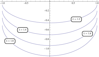
(a)

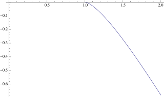
(b)

Figure 3:

Using the function $\phi_{K(\lambda)}$ constructed in Lemma 4.4 we can define a diffeomorphism in $\mathcal{C}_{\lambda}\cap\Omega$, with $\mathcal{C}_{\lambda}$ as in (2.8). Let $L\in(0,+\infty)$, we define

$$\phi_{L}(y):=L\phi_{K(\lambda)}\left(\frac{y}{L}\right),\quad y\in[-L,L].$$

We have the following Lemma.

Lemma 4.5.

(A diffeomorphism)
Let $\phi_{K(\lambda)}$ be as in (2.6), then for $(y,z)\in\overline{\mathcal{C}_{\lambda}\cap\Omega}\setminus\{(0,0)\}$ there is a unique $L=L(y,z)\in(0,+\infty)$ implicitly defined by

(4.18) $$z=L\phi_{K(\lambda)}\left(\frac{y}{L}\right)=\phi_{L}(y),$$

and $L\in C^{\infty}(\mathcal{C}_{\lambda}\cap\Omega)\cap C(\overline{\mathcal{C}_{\lambda}\cap\Omega}\setminus\{(0,0)\})$.

Proof of Lemma 4.5
  Since the family of curves $\{(y,\phi_{L}(y))\}_{L\in(0,+\infty)}$ are obtained as a rescaling of the function $\phi_{K(\lambda)}$ we have that the mapping $(y,L)\mapsto(y,z)$ is a surjection; it is also an injection since the family of curves $\{(y,\phi_{L}(y))\}_{L\in(0,+\infty)}$ do not intersect. On the other hand the same bijective correspondence can be established locally by the implicit function theorem since $\frac{y}{L}\phi_{K(\lambda)}^{\prime}\left(\frac{y}{L}\right)-\phi_{K(\lambda)}\left(\frac{y}{L}\right)>0$ (since $\phi_{K(\lambda)}$ is even and negative), from which we also get the smoothness of $L(y,z)$ in $\mathcal{C}_{\lambda}\cap\Omega$ because $\phi_{K(\lambda)}$ is smooth. The continuity of $L$ up to the boundary follows from the definition and the continuity of $\phi_{K(\lambda)}$. $\Box$

Using the diffeomorphism from Lemma 4.5 we can define $q=q_{\lambda}(y,z)\in C^{\infty}(\mathcal{C}_{\lambda}\cap\Omega,\mathbb{R}^{2})\cap C(\overline{\mathcal{C}_{\lambda}\cap\Omega}\setminus\{(0,0)\},\mathbb{R}^{2})$ as follows

(4.19) $$q(y,z):=\frac{(-\phi^{\prime}_{L(y,z)}(y),1)}{\sqrt{1+|\phi^{\prime}_{L(y,z)}(y)|^{2}}},\quad(y,z)\in\overline{\mathcal{C}_{\lambda}\cap\Omega}\setminus\{(0,0)\},$$

where $\phi^{\prime}_{L(y,z)}(y)=\phi^{\prime}_{K(\lambda)}\left(\frac{y}{L(y,z)}\right)$. Note that the boundary values of $q$ make sense because of the boundary values of $\phi^{\prime}_{K(\lambda)}$ by Lemma (2.6). We have the following Lemma

Lemma 4.6.

(An equation for $q$)
Let $\lambda>1$, $q$ as in (4.19) then

(4.20) $$-\mathrm{div}(|z|q(y,z))=\lambda,\quad\text{for }(y,z)\in(\mathcal{C}_{\lambda}\cap\Omega).$$

Proof of Lemma 4.6
  All the equations in this proof hold for $(y,z)\in\mathcal{C}_{\lambda}\cap\Omega$. Having in mind the diffeomorphism $(y,z)\mapsto(\bar{y},L(y,z))$, with $\bar{y}(y)=y$ from Lemma 4.5, we can write $q=q(\bar{y},L(y,z))=(q_{1}(\bar{y},L(y,z)),q_{2}(\bar{y},L(y,z)))$. Since $|z|=-z$ in $\Omega$, we have

(4.21) $$\mathrm{div}_{(y,z)}(|z|q)=|z|\mathrm{div}_{(y,z)}(q)-q_{2}$$

and

(4.22) $$\partial_{y}q_{1} =\partial_{\bar{y}}q_{1}+\partial_{L}(q_{1})\partial_{y}L$$

$$\partial_{z}q_{2} =\partial_{L}(q_{2})\partial_{z}L.$$

In order to simplify the notation we set $\psi=\phi_{K(\lambda)}$, then using (4.18) we can write $q_{1}=\frac{-\psi^{\prime}(y/L)}{\sqrt{1+|\psi^{\prime}(y/L)|^{2}}}$ and $q_{2}=\frac{1}{\sqrt{1+|\psi^{\prime}(y/L)|^{2}}}$, from which we can calculate

(4.23) $$\partial_{L}q_{1} =\frac{\psi^{\prime\prime}\left(\frac{y}{L}\right)\left(\frac{y}{L^{2}}\right)}{\left(1+|\psi^{\prime}\left(\frac{y}{L}\right)|^{2}\right)^{3/2}},$$

$$\partial_{L}q_{2} =\frac{\psi^{\prime\prime}\left(\frac{y}{L}\right)\psi^{\prime}\left(\frac{y}{L}\right)\left(\frac{y}{L^{2}}\right)}{\left(1+|\psi^{\prime}\left(\frac{y}{L}\right)|^{2}\right)^{3/2}}.$$

Differentiating (4.18) in $y$ and $z$ we get

(4.24) $$\partial_{z}L =\frac{-1}{\frac{y}{L}\psi^{\prime}\left(\frac{y}{L}\right)-\psi\left(\frac{y}{L}\right)},$$

$$\partial_{y}L =\frac{\psi^{\prime}\left(\frac{y}{L}\right)}{\frac{y}{L}\psi^{\prime}\left(\frac{y}{L}\right)-\psi\left(\frac{y}{L}\right)}.$$

Using (4.23), (4.24) we get $\partial_{L}(q_{1})\partial_{y}L+\partial_{L}(q_{2})\partial_{z}L=0$ and hence we get from (4.22)

(4.25) $$\mathrm{div}_{(y,z)}q=\partial_{\bar{y}}q_{1}=\frac{d}{d\bar{y}}\frac{-\phi_{L}^{\prime}(\bar{y})}{\sqrt{1+|\phi_{L}^{\prime}(\bar{y})|^{2}}}=\frac{-\phi_{L}^{\prime\prime}(\bar{y})}{(1+|\phi_{L}^{\prime}(\bar{y})|^{2})^{3/2}}.$$

Using the fact that $\bar{y}=y$, $z<0$, (4.18) and (4.25), equation (4.21) becomes

$$-\mathrm{div}_{(y,z)}(|z|q)=-\frac{\phi_{L}(y)\phi_{L}^{\prime\prime}(y)}{(1+|\phi_{L}^{\prime}(y)|^{2})^{3/2}}+\frac{1}{\sqrt{1+|\phi_{L}^{\prime}(y)|^{2}}},\quad$$

and finally using the above equation together with (4.13) and the definition of $\phi_{L}$ we conclude

$$-\mathrm{div}_{(y,z)}(|z|q)=\lambda,\quad(y,z)\in\mathcal{C}_{\lambda}\cap\Omega.$$

$\Box$

Note also that by (4.24) and the boundary conditions of $\phi^{\prime}_{K(\lambda)}$ we can extend $L\in C^{1}(\overline{\mathcal{C}_{\lambda}\cap\Omega}\setminus\{(0,0)\})$.

Lemma 4.7.

(Bound on the Laplacian)
Let $L$ be as in (4.18), then there are positive constants $C_{1},C_{2}$ such that if

(4.26) $$C=C(\lambda):=1+\left(\frac{\lambda-1}{K(\lambda)}\right)^{2}$$

we have

(4.27) $$(\partial_{y}L(y,z))^{2}+(\partial_{z}L(y,z))^{2}\leq C\quad \text{ for }(y,z)\in\mathcal{C}_{\lambda}\cap\Omega,$$

(4.28) $$L(y,z)\Delta_{(y,z)}L(y,z)\leq C_{1}+C_{2}\quad \text{ for }(y,z)\in\mathcal{C}_{\lambda}\cap\Omega,$$

in particular we have

(4.29) $$0\leq\Delta_{(y,z)}(L(y,z))^{2}\leq 2(C+C_{1}+C_{2}),\quad(y,z)\in\mathcal{C}_{\lambda}\cap\Omega.$$

Proof of Lemma 4.7
  As in the proof of Lemma 4.6 we simplify the notation by setting $\psi=\phi_{K(\lambda)}$.
Step 1. Bound on $\partial_{z}L$ and $\partial_{y}L$

By (4.14) we have $\psi^{\prime\prime}>0$ in $(-1,1)$, then, using also (4.15) we can estimate by the maximum

(4.30) $$\frac{1}{y\psi^{\prime}(y)-\psi(y)}\leq\frac{\lambda-1}{-K(\lambda)},\quad\text{ for }y\in(-1,1).$$

Let $(y,z)\in\mathcal{C}_{\lambda}\cap\Omega$, by the diffeomorphism in Lemma 4.5 we have $\frac{|y|}{L(y,z)}\leq 1$, hence using (4.30) and the formula of $\partial_{z}L$ by (4.24) we have $|\partial_{z}L(y,z)|\leq\frac{\lambda-1}{-K(\lambda)}$.

Similarly for $\partial_{y}L$ given by the formula (4.24), since

$$\frac{d}{dy}\left(\frac{\psi^{\prime}(y)}{y\psi^{\prime}(y)-\psi(y)}\right)=\frac{-\psi(y)\psi^{\prime\prime}(y)}{(y\psi^{\prime}(y)-\psi)^{2}}>0\,\quad\text{ for }y\in(-1,1),$$

and $\displaystyle\lim_{y\rightarrow 1}\frac{\psi^{\prime}(y)}{y\psi^{\prime}(y)-\psi(y)}=1$, we have $|\partial_{y}L(y,z)|\leq 1$ for $(y,z)\in\mathcal{C}_{\lambda}\cap\Omega$. Combining the bounds of $\partial_{z}L$ and $\partial_{y}L$ we get (4.27).
Step 2. Bound on second derivatives

If we differentiate (4.18) twice in $z$ and $y$ respectively and use (4.24) we get

(4.31) $$L\partial^{2}_{zz}L=\frac{\psi^{\prime\prime}\left(\frac{y}{L}\right)\left(\frac{y}{L}\right)^{2}}{\left(\frac{y}{L}\psi^{\prime}\left(\frac{y}{L}\right)-\psi\left(\frac{y}{L}\right)\right)^{3}}$$

and

(4.32) $$L\partial^{2}_{yy}L=\frac{\psi^{\prime\prime}\left(\frac{y}{L}\right)\psi^{2}\left(\frac{y}{L}\right)}{\left(\frac{y}{L}\psi^{\prime}\left(\frac{y}{L}\right)-\psi\left(\frac{y}{L}\right)\right)^{3}}.$$

We estimate in $\mathcal{C}_{\lambda}\cap\Omega$

$$L\partial^{2}_{zz}L\leq\max\left\{\max_{\frac{|y|}{L}\leq\frac{1}{2}}L\partial^{2}_{zz}L,\sup_{\frac{1}{2}<\frac{|y|}{L}<1}L\partial^{2}_{zz}L\right\}.$$

Using the fact that $y\psi^{\prime}(y)\geq 0$ and the maximum of $\psi$ by (4.15) we estimate

(4.33) $$\max_{\frac{|y|}{L}\leq\frac{1}{2}}L\partial^{2}_{zz}L\leq\frac{1}{4}\left(\frac{\lambda}{-K(\lambda)}\right)^{3}\displaystyle\max_{|y|\leq\frac{1}{2}}\psi^{\prime\prime}(y).$$

For $1/2<|y/L|<1$ it is $\psi^{\prime}\neq 0$ and we can rewrite (4.31) as

(4.34) $$L\partial^{2}_{zz}L=\frac{\psi^{\prime\prime}\left(\frac{y}{L}\right)}{\left|\psi^{\prime}\left(\frac{y}{L}\right)\right|^{3}}\cdot\frac{\left(\frac{y}{L}\right)^{2}}{\left(\left|\frac{y}{L}\right|+\frac{-\psi\left(\frac{y}{L}\right)}{\left|\psi^{\prime}\left(\frac{y}{L}\right)\right|}\right)^{3}},$$

and by equation (4.14) we calculate in the same interval

(4.35) $$\frac{\psi^{\prime\prime}}{|\psi^{\prime}|^{3}}=\frac{\lambda\left(\frac{1}{|\psi^{\prime}|^{2}}+1\right)^{3/2}-\frac{1}{|\psi^{\prime}|^{3}}-\frac{1}{|\psi^{\prime}|}}{-\psi}.$$

Substituting (4.35) in (4.34) and using properties of $\psi$ and the monotonicity of $\psi^{\prime}$ we get the bound

(4.36) $$\sup_{\frac{1}{2}<\frac{|y|}{L}<1}L\partial^{2}_{zz}L\leq\frac{2\lambda^{2}}{-K(\lambda)}\left(\frac{1}{\left|\psi^{\prime}\left(\frac{1}{2}\right)\right|^{2}}+1\right)^{3/2}.$$

Finally by (4.36) and (4.33) we get $\displaystyle\sup_{\mathcal{C}_{\lambda}\cap\Omega}L\partial^{2}_{zz}L\leq C_{1}$, with $C_{1}$ a positive constant. Similarly one can show that $\displaystyle\sup_{\mathcal{C}_{\lambda}\cap\Omega}L\partial^{2}_{yy}L\leq C_{2}$ with

$$C_{2}=\max\left\{\frac{\lambda}{-K(\lambda)}\max_{|y|\leq\frac{1}{2}}\psi^{\prime\prime}(y),8\left(\frac{\lambda}{\lambda-1}\right)^{2}(-K(\lambda))\left(\frac{1}{\left|\psi^{\prime}\left(\frac{1}{2}\right)\right|^{2}}+1\right)^{3/2}\right\}.$$

$\Box$

4.3 A subsolution

Remark 4.8.

Let $\sigma:\Omega_{1}\cup\Omega_{2}\rightarrow\mathbb{R}^{2}$, with $\Omega_{1},\Omega_{2}\subset\mathbb{R}^{2}$, two bounded domains with Lipschitz boundary and a common smooth boundary $\partial\Omega$, with surface measure $dS$. Suppose that $\sigma\in\displaystyle\bigcap_{i=1}^{2}(C^{1}(\Omega_{i},\mathbb{R}^{2})\cap C(\overline{\Omega_{i}},\mathbb{R}^{2}))$, $\mathrm{div}\sigma\in L^{2}(\Omega_{1})\cap L^{2}(\Omega_{2})$, we denote by $\mathrm{Tr}\mid_{\Omega_{i}}\sigma$, $i=1,2$, the limit value of $\sigma$ from the sides $\Omega_{i}$ respectively. Then for $\phi\in W^{1,2}_{0}(\Omega_{1}\cup\Omega_{2})$ with $\mathrm{supp}(\phi)\cap\partial\Omega\neq\emptyset$ it is

(4.37) $$\int_{\Omega_{1}\cup\Omega_{2}}\sigma\cdot\nabla\phi=-\int_{\Omega_{1}\cup\Omega_{2}}\mathrm{div}(\sigma)\phi+\int_{\partial\Omega}n\cdot(\mathrm{Tr}\mid_{\Omega_{1}}\sigma-\mathrm{Tr}\mid_{\Omega_{2}}\sigma)\phi\,dS$$

where $n$ is the normal to $\partial\Omega$ pointing at the direction of $\Omega_{2}$.

We can now construct a subsolution. In what follows we will favour intuition over mathematical elegance, as far as the notation is concerned, and we will instead denote the set $\mathrm{Epi}^{\smallsmile}(\lambda)$ defined in (2.9), simply by $\{z>\phi_{K(\lambda)}\}$. Let $\zeta>0$, using the diffeomorfism from Lemma 4.5 we can define the continuous function (see Figure 4)

(4.38) $$u_{\zeta,\lambda}(y,z):=\begin{cases}-\zeta y^{2}+\zeta&\text{ in }\Omega\setminus\mathcal{C}_{\lambda},\\ -\zeta L^{2}(y,z)+\zeta&\text{ in }\mathcal{C}_{\lambda}\cap\{z\geq\phi_{K(\lambda)}\},\\ 0&\text{ in }\{z<\phi_{K(\lambda)}\},\end{cases}$$

and for $q_{\lambda}$ as in (4.19) we define

(4.39) $$d^{\mathrm{ext}}_{\lambda}(y,z):=\begin{cases}\left(-\frac{y}{|y|},0\right)&\text{ in }\Omega\setminus\mathcal{C}_{\lambda},\\ q_{\lambda}(y,z)&\text{ in }\mathcal{C}_{\lambda}\cap\Omega.\end{cases}$$

Then we have that $u_{\zeta,\lambda}\in\mathcal{X}$ with $\partial_{z}u_{\zeta,\lambda}(y,0)=0$ for $y\in(-1,1)$ and $d^{\mathrm{ext}}_{\lambda}\in\Lambda$. In the set $\mathcal{C}_{\lambda}\cap\{z>\phi_{K(\lambda)}\}$ we have $\nabla u_{\zeta,\lambda}=-2\zeta L(\partial_{y}L,\partial_{z}L)$, then using also (4.24), (4.38), (4.39), definition (4.19) and the properties of $\phi_{K(\lambda)}$ by Lemma 4.4 we have that $d^{\mathrm{ext}}_{\lambda}\cdot\nabla u_{\zeta,\lambda}=|\nabla u_{\zeta,\lambda}|$ a.e. in $\Omega$.

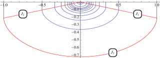
(a)

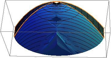
(b)

Figure 4:

Proposition 4.9.

(Subsolution)
Let $\lambda>1$, then there is $1<\lambda_{0}<\lambda$ such that for $0<\zeta_{0}\leq\frac{\lambda-\lambda_{0}}{2(C+C_{1}+C_{2})}$, with $C,C_{1},C_{2}$ given by Lemma 4.7, the pair $(u_{\zeta_{0},\lambda_{0}},d^{\mathrm{ext}}_{\lambda_{0}})$ given by (4.38)-(4.39), is a subsolution of the equation (2.3).

Proof of Proposition 4.9
  Step 1. The subsolution inequalities

We will first show the subsolution inequalities in the set

$$\Omega_{1}\cup\Omega_{2}\cup\Omega_{3}:=\left(\Omega\setminus\overline{\mathcal{C}_{\lambda_{0}}}\right)\cup\left(\mathcal{C}_{\lambda_{0}}\cap\{z>\phi_{K(\lambda_{0})}\}\right)\cup\left(\mathcal{C}_{\lambda_{0}}\setminus\{z\geq\phi_{K(\lambda_{0})}\}\right)$$

where the functions $u_{\zeta_{0},\lambda_{0}},\,d^{\mathrm{ext}}_{\lambda_{0}}$ are smooth. Using (4.20) and (4.39) we calculate

(4.40) $$-\mathrm{div}(|z|d^{\mathrm{ext}}_{\lambda_{0}}(y,z))=\begin{cases}0&\text{ in }\Omega\setminus\overline{\mathcal{C}_{\lambda_{0}}},\\ \lambda_{0}&\text{ in }\mathcal{C}_{\lambda_{0}}\cap\Omega.\end{cases}$$

Also

(4.41) $$-\Delta u_{\zeta_{0},\lambda_{0}}=\begin{cases}2\zeta_{0}&\text{ in }\Omega\setminus\overline{\mathcal{C}_{\lambda_{0}}},\\ 0&\text{ in }\Omega\cap\{z<\phi_{K(\lambda_{0})}\}.\end{cases}$$

and using Lemma 4.7 we get in $\mathcal{C}_{\lambda_{0}}\cap\{z>\phi_{K(\lambda_{0})}\}$

(4.42) $$-\Delta u_{\zeta_{0},\lambda_{0}}=\zeta_{0}\Delta L^{2}\leq 2\zeta_{0}(C+C_{1}+C_{2})$$

If we now combine (4.40)-(4.42), use the fact that the positive constant $2(C+C_{1}+C_{2})$ depends only on $\lambda_{0}$, we can choose $\zeta_{0}\leq\frac{\lambda-\lambda_{0}}{2(C+C_{2}+C_{2})}$($<\lambda/2$ since $C+C_{1}+C_{2}>1$ by (4.26)) and get

(4.43) $$-\Delta u_{\zeta_{0},\lambda_{0}}-\mathrm{div}(|z|d^{\mathrm{ext}}_{\lambda_{0}})\leq\lambda\quad\text{ in }\Omega_{1}\cup\Omega_{2}\cup\Omega_{3}.$$

It remains to show that inequality (4.43) holds in the rest of $\Omega$. We will use Remark 4.8 for $\sigma=\nabla u_{\zeta_{0},\lambda_{0}}+|z|d^{\mathrm{ext}}_{\lambda_{0}}$. Note that $\sigma$ is not defined at $(0,0)$ but we still have that it is bounded near $z=0$ by Lemma 4.7.
Step 2. The Dirac masses

Note that since $\partial_{z}u_{\zeta_{0},\lambda_{0}}(y,0)=0$ and therefore $\sigma(y,0)=0$, for $y\in(-1,1)\setminus\{(0,0)\}$, in view of (4.37), we do not need to take into account the boundary $\{z=0\}$. We denote by $J=J_{1}\cup J_{2}\cup J_{3}$ the three parts of the boundary of $\Omega_{1}\cup\Omega_{2}\cup\Omega_{3}$ as in Figure (4a). We will show the subsolution inequalities on $J$. We need to estimate for $(i,j)\in\{(1,2),(2,3)\}$, the terms

(4.44) $$n_{j}\cdot\left(\mathrm{Tr}\mid_{\Omega_{i}}\sigma-\mathrm{Tr}\mid_{\Omega_{j}}\sigma\right),$$

where $n_{j}$ is the normal of the common boundary pointing in the direction of $\Omega_{j}$. For $J_{1}$, the right common boundary of $\Omega_{1}$ and $\Omega_{2}$ we have $n_{1}=\left(\frac{K(\lambda_{0})}{\lambda_{0}},-1\right)$, using (4.4) and (4.19) one can see that that $d^{\mathrm{ext}}_{\lambda}$ is continuous in $\Omega$, therefore using (4.38) we get

(4.45) $$\mathrm{Tr}\mid_{\Omega_{1}}\sigma-\mathrm{Tr}\mid_{\Omega_{2}}\sigma=(-2\zeta_{0}y,0)+2\zeta_{0}L(\partial_{y}L,\partial_{z}L)=0,\quad(y,z)\in J_{1},$$

where we used the fact that $y=L$ on $J_{1}$ and $(\partial_{y}L,\partial_{z}L)=(1,0)$ by the Neumann conditions in (4.4). In a similar way we can write (4.44) on $J_{2}$ as

(4.46) $$-n_{2}\cdot\left(\mathrm{Tr}\mid_{\Omega_{1}}\sigma-\mathrm{Tr}\mid_{\Omega_{2}}\sigma\right)=0.$$

where $n_{2}=\left(\frac{-K(\lambda_{0})}{\lambda_{0}},-1\right)$. On $J_{3}$ we simplify the notation and set $\psi=\phi_{K(\lambda_{0})}$, then (4.44) becomes

(4.47) $$n_{3}\cdot\left(\mathrm{Tr}\mid_{\Omega_{2}}\sigma-\mathrm{Tr}\mid_{\Omega_{3}}\sigma\right) =\left(\frac{\psi^{\prime}}{\sqrt{1+|\psi^{\prime}|^{2}}},\frac{-1}{\sqrt{1+|\psi^{\prime}|^{2}}}\right)\cdot\left(-2\zeta_{0}L(\partial_{y}L,\partial_{z}L)\right)$$

$$=-2\zeta_{0}\frac{\sqrt{1+|\psi^{\prime}|^{2}}}{y\psi^{\prime}-\psi}\leq 0,$$

where in the last equality we used equations (4.24) and that $L=1$ on $J_{3}$. We can now conclude from estimates (4.45), (4.46) and (4.47). $\Box$

Proof of Theorem 2.3 (lower bound)
  If we compare the subsolution $u_{\zeta_{0},\lambda_{0}}$ by Proposition 4.9 with the solution $u_{\lambda}$ of (2.3) using Proposition 4.2, we get $0\leq u_{\zeta_{0},\lambda_{0}}\leq u_{\lambda}$ in $\Omega$ for all $\lambda_{0}\in(1,\lambda)$, hence by definitions (4.38) and (2.9) we get

(4.48) $$\{u_{\zeta_{0},\lambda_{0}}>0\}=\{z>\phi_{K(\lambda_{0})}\}=\mathrm{Epi}^{\smallsmile}(\lambda_{0})\subset\{u_{\lambda}>0\},\quad\text{ for all }\lambda_{0}\in(1,\lambda).$$

We set $\psi(y,\lambda)=\phi_{K(\lambda)}(y)$ for $(y,\lambda)\in[0,1]\times(1,+\infty)$. By definition (2.6) we have that $\psi$ satisfies the equation $F(y,\lambda,\psi(y,\lambda))=0$ with

$$F:\{(y,\lambda,z):\,y\in(0,1),\,\lambda\in(1,+\infty),\,z\in\left(\frac{K(\lambda)}{\lambda-1},\frac{K(\lambda)}{\lambda}\right)\}\rightarrow\mathbb{R}$$

given by

$$F(y,\lambda,z)=K(\lambda)f_{\lambda}\left(\frac{z}{K(\lambda)}\right)-K(\lambda)f_{\lambda}\left(\frac{1}{\lambda-1}\right)-y.$$

The using the formulas (2.5), (2.7) and (4.6) one can check that $F$ is smooth in the domain of it’s definition. Since $f^{\prime}_{\lambda}\left(\frac{\psi(y,\lambda)}{K(\lambda)}\right)>0$ for $(y,\lambda)\in(0,1)\times(1,+\infty)$ we have by the implicit function theorem that $\psi\in C^{\infty}((0,1)\times(1,+\infty))$. Since $\phi_{K(\lambda)}$ is even, we get that for fixed $y\in(-1,0)\cup(0,1)$ the function $\phi_{K(\lambda)}(y)$ is continuous in $\lambda$ in $(1,+\infty)$. By the formulas of $\phi_{K(\lambda)}(\pm 1)$, $\phi_{K(\lambda)}(0)$ by Lemma (4.4) and the continuity of the function $K(\lambda)$ we get that $\displaystyle\lim_{\lambda_{0}\uparrow\lambda}\phi_{K(\lambda_{0})}(y)=\phi_{K(\lambda)}(y)$ for all $y\in[-1,1]$. We can now pass to the limit in (4.48) and conclude. $\Box$

4.4 A supersolution

Let $\lambda>1$, $\lambda_{1}>\lambda$ and $\vartheta,b,\Pi$ given by (2.10), (2.11), (2.12) respectively. Using the diffeomorphism from Lemma 4.5 with $\phi_{K(\lambda_{1})}$ in (4.18) we can consider sets of the form $\{(y,z)\in\mathcal{C}_{\lambda}\cap\Omega:\,1\leq L(y,z)\leq b\}$, where the level set $\{(y,z)\in\mathcal{C}_{\lambda}\cap\Omega:\,L(y,z)=1\}$ is the graph $\{z=\phi_{K(\lambda_{1})}\}$; we will simply denote by $\{1\leq L(y,z)\leq b\}$ these sets. We define

(4.49) $$u_{1}^{\lambda_{1}}(y,z):=\frac{\lambda_{1}}{2}(1-y^{2}),\quad(y,z)\in\Omega,$$

(4.50) $$u_{2}^{\lambda_{1},\vartheta}(y,z):=\begin{cases}+\infty&\text{ in }\{z>\phi_{K(\lambda_{1})}\},\\ \vartheta(L(y,z)-b)^{2}&\text{ in }\{1\leq L(y,z)\leq b\},\\ 0&\text{ in }\{b\leq L(y,z)\}.\end{cases}$$

where we simply write $\vartheta$ for $\vartheta_{\lambda,\lambda_{1}}$. Also, we define

(4.51) $$U^{\lambda_{1},\vartheta}=\min\{u_{1}^{\lambda_{1}},u_{2}^{\lambda_{1},\vartheta}\},\quad\text{ in }\Omega.$$

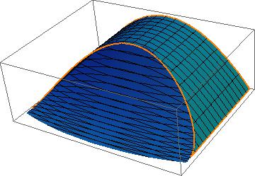
Figure 5: $U^{\lambda_{1},\vartheta}$

We note that the intersection of the graphs of the functions $u_{2}^{\lambda_{1},\vartheta}$ and $u_{1}^{\lambda_{1}}$ lies in the domain $\Omega\cap\{L(y,z)<b\}$ and is given by the equation

(4.52) $$\vartheta(L(y,z)-b)^{2}=\frac{\lambda_{1}}{2}(1-y^{2}),\quad(y,z)\in\Omega\cap\{L(y,z)<b\},$$

or else since $L<b$

$$L(y,z)=b-\sqrt{\frac{\lambda_{1}}{2\vartheta}(1-y^{2})}\geq b-\sqrt{\frac{\lambda_{1}}{2\vartheta}}=1,$$

by the definition of $b$. Also, since $\partial_{z}L<0$ in $\mathcal{C}_{\lambda}\cap\Omega$ the curve defined by the contour (4.52) is the graph of a function which lies in fact in the set $\{1\leq L(y,z)\leq b\}$, and therefore, the function $U^{\lambda_{1},\vartheta}$ is continuous, see Figure 5. For $q_{\lambda_{1}}$ as in (4.19) we define for a.e. $y\in\Omega$ the vector field

(4.53) $$q^{\mathrm{ext}}_{\lambda_{1}}(y,z):=\left\{\begin{aligned} &\left(-\frac{y}{|y|},0\right)&\text{ in }&(\{1\leq L(y,z)<b-\sqrt{\frac{\lambda_{1}}{2\vartheta}(1-y^{2})}\}\cup\{z>\phi_{K(\lambda_{1})}\})\cap\{y\neq 0\}\\ &q_{\lambda_{1}}(y,z)&\text{ in }&\{b-\sqrt{\frac{\lambda_{1}}{2\vartheta}(1-y^{2})}<L(y,z)\}.\end{aligned}\right.$$

We have the following Proposition.

Proposition 4.10.

(Supersolution)
Let $\lambda>1$, then the function $U^{\lambda_{1},\vartheta}$ defined in (4.51) is a supersolution of (2.3).

Proof of Proposition 4.10
  A straightforward calculation shows that $\nabla U^{\lambda_{1},\vartheta}\cdot q^{\mathrm{ext}}_{\lambda_{1}}=|\nabla U^{\lambda_{1},\vartheta}|$, a.e. in $\Omega$. We also have $\partial_{z}U^{\lambda_{1},\vartheta}(y,0)=\partial_{z}u_{1}^{\lambda_{1}}(y,0)=0$.
Step 1. Supersolution inequalities

It is

$$-\Delta U^{\lambda_{1},\vartheta}=\left\{\begin{aligned} &\lambda_{1}&\text{ in }&\{1\leq L(y,z)<b-\sqrt{\frac{\lambda_{1}}{2\vartheta}(1-y^{2})}\}\cup\{z>\phi_{K(\lambda_{1})}\}\\ &-2\vartheta((\partial_{y}L)^{2}+(\partial_{z}L)^{2})&&\\ &\quad+2\vartheta(b-L)(\partial^{2}_{yy}L+\partial^{2}_{zz}L)&\quad\text{ in }&\{b-\sqrt{\frac{\lambda_{1}}{2\vartheta}(1-y^{2})}<L(y,z)<b\}\\ &0&\quad\text{ in }&\{b<L(y,z)\},\end{aligned}\right.$$

and as in (4.40) we have

$$-\mathrm{div}(|z|q^{\mathrm{ext}}_{\lambda_{1}})=\left\{\begin{aligned} &0&\quad\text{ in }&(\{1\leq L(y,z)<b-\sqrt{\frac{\lambda_{1}}{2\vartheta}(1-y^{2})}\}\cup\{z>\phi_{K(\lambda_{1})}\})\cap\{y\neq 0\}\\ &\lambda_{1}&\quad\text{ in }&\{b-\sqrt{\frac{\lambda_{1}}{2\vartheta}(1-y^{2})}<L(y,z)\}.\end{aligned}\right.$$

Therefore if $C$ is as in (4.26), we have $\vartheta=\frac{\lambda_{1}-\lambda}{2C}$ and

$$-\Delta U_{\lambda_{1},\vartheta}-\mathrm{div}(|z|q^{\mathrm{ext}}_{\lambda_{1}})\geq\lambda,\quad\text{ in }\Omega\setminus(\{L(y,z)=b-\sqrt{\frac{\lambda_{1}}{2\vartheta}(1-y^{2})}\}\cup\{0\}\times\left(\frac{K(\lambda_{1})}{\lambda_{1}-1},0\right)).$$

Note that the solution of the equation $L(0,z)=1$ is $z=\frac{K(\lambda_{1})}{\lambda_{1}-1}$. We also note that by (4.31), (4.32) and Step 2 of the proof of Lemma 4.7 we have that $\Delta U_{\theta,\lambda_{1}}$ is bounded.
Step 2. Dirac masses

The discontinuities of the vector fields $\nabla U_{\lambda_{1},\vartheta}$ and $q^{\mathrm{ext}}_{\lambda_{1}}$ lie on the intersection given by the contour (4.52) and on $\{0\}\times\left(\frac{K(\lambda_{1})}{\lambda_{1}-1},0\right)$. For the second set only the vector field $q^{\mathrm{ext}}_{\lambda_{1}}$ is discontinuous and the Dirac mass it creates is

$$|z|(1,0)\cdot((1,0)-(-1,0))\geq 0.$$

For the intersection, eq. (4.52), we suppress the indices $\lambda_{1},\vartheta$ and we write the Dirac mass as

(4.54) $$n\cdot\left[(\nabla u_{1}-\nabla u_{2})+|z|\left(\frac{\nabla u_{1}}{|\nabla u_{1}|}-\frac{\nabla u_{2}}{|\nabla u_{2}|}\right)\right],$$

where $n$ is the normal to the intersection pointing at the direction of $\{L(y,z)>b-\sqrt{\frac{\lambda_{1}}{2\vartheta}(1-y^{2})}\}$. Then the $z-$component of $n$ is negative, and since $L_{z}<0$ by (4.24) we have

$$n=\frac{\nabla u_{1}-\nabla u_{2}}{|\nabla u_{1}-\nabla u_{2}|}.$$

Clearly we have $n\cdot(\nabla u_{1}-\nabla u_{2})\geq 0$. The second term of (4.54) is

$$\frac{|z|}{|\nabla u_{1}-\nabla u_{2}|}\left(|\nabla u_{1}|+|\nabla u_{2}|-\nabla u_{1}\cdot\nabla u_{2}\frac{|\nabla u_{1}|+|\nabla u_{2}|}{|\nabla u_{1}||\nabla u_{2}|}\right)\geq 0$$

by the Cauchy-Schwartz inequality. This concludes the proof. $\Box$

Proof of Theorem 2.3 (upper bound)
  We will estimate $\mathrm{supp}\,u$ from above. By Propositions 4.10 and 4.2 we get $0\leq u_{\lambda}\leq U_{\lambda_{1},\vartheta}$ in $\Omega$ and since $\mathrm{supp}\,U_{\lambda_{1},\vartheta}=\mathrm{Epi}_{\smallsmile}(\lambda_{1})$ we get the desired estimate. $\Box$

Let $\lambda^{\star}_{1}=\lambda^{\star}_{1}(\lambda)>\lambda$ be a minimizer of $\Pi(\lambda,\cdot)$ (see discussion before Theorem 2.3). In Figure 6 we give the graph of $\Pi(\lambda,\lambda^{\star}_{1})$ for different values of $\lambda$ and in Table 1 the corresponding minimizers and minimal values. In fact one notices that the difference $\lambda^{\star}_{1}-\lambda$ increases as $\lambda\rightarrow+\infty$, see Figure 7a.

$\lambda=1.2$	$\lambda^{\star}_{1}=1.59451$	$\Pi=3.20584$
$\lambda=1.4$	$\lambda^{\star}_{1}=1.84198$	$\Pi=3.66274$
$\lambda=1.6$	$\lambda^{\star}_{1}=2.09337$	$\Pi=4.16455$
$\lambda=1.8$	$\lambda^{\star}_{1}=2.34819$	$\Pi=4.69225$

Table 1: Optimal $\lambda^{\star}_{1}$

Figure 6: $\Pi(\lambda,\lambda^{\star}_{1})$ for $\lambda=1.2,\,1.4,\,1.6,\,1.8$

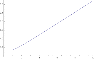
(a)

(b)

Figure 7:

A Regularity of $\varepsilon$-minimizers

In what follows we will denote by $c$ a generic constant which does not depend on the $\varepsilon$ mentioned in Proposition 3.5.

Proof of Proposition 3.5
  Step 1. Existence/Uniqueness

The uniqueness of the minimizer follows by the strict convexity of the functional or using similar arguments as in the proof of Step 1 of Theorem 2.2 (i). The existence is also similar, in fact the lower semicontinuity of the linear term $-\lambda\int_{\Omega_{A}}u$ is trivial since the domain $\Omega_{A}$ is bounded. We set

(A.1) $$F(z,p)=\frac{|p|^{2}}{2}+|z|\sqrt{\varepsilon^{2}+|p|^{2}},$$

for $(z,p)\in\Omega_{A}\times\mathbb{R}^{2}$. It is

(A.2) $$|\xi|^{2}\leq\frac{\partial^{2}F}{\partial p_{i}\partial p_{j}}\xi_{i}\xi_{j}$$

for $\xi=(\xi_{1},\xi_{2})\in\mathbb{R}^{2}$, and

(A.3) $$\left|\frac{\partial^{2}F}{\partial p_{i}\partial p_{j}}\right|\leq c\left(1+\frac{A}{\varepsilon}\right),\text{ for all }i,j\in\{1,2\},$$

we set $c_{2}:=c\left(1+\frac{A}{\varepsilon}\right)$.
Step 3. Regularity

Since the proof of regularity is standard we are only going to emphasize the particularities of the problem, i.e. the fact that $F$ is only Lipschitz continuous in the $z$ variable. We will simply write $F(z,\nabla u)$ for $F(z,\nabla u(y,z))$. Let $\varphi$ with $\hat{\varphi}\in W^{1,2}_{0}(\hat{\Omega}_{A})$, then equation (3.35) holds as the first variation of the functional $E^{A}_{\varepsilon,\lambda}$. Moreover, using a change of variables one can see that the function $w:=\hat{u}_{\varepsilon,A}$ satisfies

(A.4) $$\int_{\hat{\Omega}_{A}}\nabla w\cdot\nabla\varphi+|z|\frac{\nabla w\cdot\nabla\varphi}{\sqrt{\varepsilon^{2}+|\nabla w|^{2}}}=\lambda\int_{\hat{\Omega}_{A}}\varphi.$$

We study the regularity properties of (A.4). Let $|h|<\mathrm{dist}(\mathrm{supp}\,\varphi,\partial\hat{\Omega}_{A})$, we define $\varphi_{k,h}(y,z):=\varphi((y,z)-he_{k}),\,k=1,2$, with $e_{k},\,k=1,2$ the unit vectors on the axes $y$ and $z$ respectively. We use $\varphi_{k,h}$ as a test function in (A.4) and estimate the derivative of the difference quotient

(A.5) $$\Delta_{h}^{k}w(y,z)=\frac{w((y,z)+he_{k})-w(y,z)}{h}.$$

Since the proof is similar we will only present the estimate for $e_{2}$. Using $\varphi_{2,h}=\varphi_{h}$ as a test function in (A.4) and after changing the variables in the integral we get

(A.6) $$\int_{\hat{\Omega}_{A}}\partial_{p_{i}}F(z+h,(\nabla w)_{h})\partial_{x_{i}}\varphi=\lambda\int_{\hat{\Omega}_{A}}\varphi,$$

where $\partial_{p_{i}}F=\frac{\partial F}{\partial p_{i}}$, $(\nabla w)_{h}(y,z)=\nabla w(y,z+h)$ and $\partial_{x_{i}}\varphi$, $i=1,2$ is the partial derivative of $\varphi$ in the directions $y,z$ respectively. As usual subtracting (A.4) from (A.6) we get after a few calculations

(A.7) $$\int_{\hat{\Omega}_{A}}\frac{1}{h}(\partial_{p_{i}}F(z+h,(\nabla w)_{h})-\partial_{p_{i}}F(z+h,\nabla w))\partial_{x_{i}}\phi=-\int_{\hat{\Omega}_{A}}\frac{1}{h}(\partial_{p_{i}}F(z+h,\nabla w)-\partial_{p_{i}}F(z,\nabla w))\partial_{x_{i}}\phi.$$

The right hand side of (A.7) can be estimated using the Lipschitz continuity of $\nabla_{p}F$ in the $z$ variable, we have

$$\frac{1}{|h|}|\nabla_{p}F(z+h,\nabla w)-\nabla_{p}F(z,\nabla w)|=\frac{|\nabla w|}{\sqrt{\varepsilon^{2}+|\nabla w|^{2}}}\frac{||z+h|-|z||}{|h|}\leq 1.$$

It is now a standard process to use (A.2) and (A.3) in order to bound the quantity $\int|\nabla\Delta_{h}w|^{2}$ uniformly in $h$, we have

(A.8) $$\int_{\Omega^{\prime}}|\nabla\Delta_{h}w|^{2}\leq 2c_{3}(1+2c_{2})\int_{\Omega_{A}}|\nabla w|^{2},$$

with $c_{3}$ a constant independent of $h$ and $\Omega^{\prime}\subset\subset\Omega^{\prime\prime}\subset\subset\Omega_{A}$. We then have $w\in W^{2,2}(\Omega^{\prime\prime})$ by standard arguments.
Step 4. Neumann condition

Since $\hat{u}_{\varepsilon}\in W^{2,2}_{\mathrm{loc}}(\hat{\Omega}_{A})$ we can define $\partial_{z}u_{\varepsilon}(y,0)$ for a.e. $y\in(-1,1)$ and since $\hat{u}$ is symmetric with respect to $\{z=0\}$, it is in fact $\partial_{z}u_{\varepsilon}(y,z)=-\partial_{z}u_{\varepsilon}(y,-z)$ for $(y,z)\in\hat{\Omega}_{A}$; setting $z=0$ we get the desired result. $\Box$

The constant $c_{2}$ in the estimate (A.8) depends on $\varepsilon$. Using an argument similar to the proof of [8, Theorem 3.3.4] we can show that the second derivative of $u_{\varepsilon}$ is bounded in $L^{2}$, uniformly in $\varepsilon$. We have the following Lemma.

Lemma A.1.

(Uniform bound on $|\nabla^{2}u_{\varepsilon}|$)
Let $A>0$, $u_{\varepsilon}$ as in Proposition 3.5 and $\Omega^{\prime}\subset\subset\Omega^{\prime\prime}\subset\subset\hat{\Omega}_{A}$. Then there exists a positive constant $C=C(A,\mathrm{dist}(\Omega^{\prime},\partial\hat{\Omega}_{A}))$ such that

(A.9) $$\int_{\Omega^{\prime}}|\nabla\partial_{x_{i}}\hat{u}_{\varepsilon}|^{2}\leq C(1+\int_{\hat{\Omega}_{A}}|\partial_{x_{i}}\hat{u}_{\varepsilon}|^{2}),\quad i=1,2.$$

Proof of Lemma A.1
  Since the proof is similar to the proof of Proposition 3.5, we will only give a sketch of it. We will only show the proof of the estimate (A.9) for $|\nabla\partial_{z}\hat{u}_{\varepsilon}|$ because the term with the partial derivative in the $y$ variable is easier to estimate, since the integrand $F$ from (A.1) does not depend on $y$. Let $\varphi$ be a smooth function with compact support in $\Omega^{\prime\prime}$; using $\partial_{z}\varphi$ as a test function in (A.4) and integrating by parts we can write, using the usual summation convention and the same notation as in the proof of Proposition 3.5

(A.10) $$\int_{\Omega^{\prime\prime}}\partial_{p_{i}}\partial_{z}F(z,\nabla\hat{u}_{\varepsilon})\partial_{x_{i}}\varphi=0.$$

Or if we notice that $\partial_{z}\left(F(z,\nabla\hat{u}_{\varepsilon}(y,z))\right)=\partial_{\bar{z}}F(\bar{z},\nabla\hat{u}_{\varepsilon}(y,z))\mid_{\bar{z}=z}+\partial_{p_{j}}F(z,\nabla\hat{u}_{\varepsilon}(y,z))\partial_{x_{j}}\partial_{z}\hat{u}_{\varepsilon}(y,z)$ and if $\partial_{z}|z|=\chi_{(0,+\infty)}-\chi_{(-\infty,0)}$, we may rewrite (A.10) as

(A.11) $$\int_{\Omega^{\prime\prime}}\partial_{z}|z|\frac{\partial_{x_{i}}\hat{u}_{\varepsilon}}{\sqrt{\varepsilon^{2}+|\nabla\hat{u}_{\varepsilon}|^{2}}}\partial_{x_{i}}\varphi+\int_{\Omega^{\prime\prime}}\left(\partial_{p_{i}}\partial_{p_{j}}F(z,\nabla\hat{u}_{\varepsilon})\partial_{x_{j}}\partial_{z}\hat{u}_{\varepsilon}\right)\partial_{x_{i}}\varphi=0.$$

As usual we choose a function $\eta\in C^{2}_{0}(\Omega^{\prime\prime})$ with $\eta=1$ in $\Omega^{\prime}$ , $0\leq\eta\leq 1$, $|\nabla\eta|\leq\frac{c}{\mathrm{dist}(\Omega^{\prime},\partial\Omega_{A})}$ and $||\nabla^{2}\eta||\leq\frac{c}{(\mathrm{dist}(\Omega^{\prime},\partial\Omega_{A})^{2}}$. We set $\varphi=\eta^{3}\partial_{z}\hat{u}_{\varepsilon}$ in (A.11), use the convexity property (A.2) and the fact that

$$\partial_{p_{i}}\partial_{p_{j}}F(z,\nabla\hat{u}_{\varepsilon})\partial_{x_{j}}\partial_{z}\hat{u}_{\varepsilon}=\partial_{x_{i}}\partial_{z}\hat{u}_{\varepsilon}+|z|\partial_{z}\left(\frac{\partial_{x_{i}}\hat{u}_{\varepsilon}}{\sqrt{\varepsilon^{2}+|\nabla\hat{u}_{\varepsilon}|^{2}}}\right),$$

we get as in the proof of Proposition 3.5

(A.12) $$\int_{\Omega^{\prime\prime}}\eta^{3}|\nabla\partial_{z}\hat{u}_{\varepsilon}|^{2}\leq-\int_{\Omega^{\prime\prime}}\partial_{x_{i}}\partial_{z}\hat{u}_{\varepsilon}\partial_{x_{i}}(\eta^{3})\partial_{z}\hat{u}_{\varepsilon}-\int_{\Omega^{\prime\prime}}\partial_{z}|z|\partial_{x_{i}}(\eta^{3})\frac{\partial_{x_{i}}\hat{u}_{\varepsilon}}{\sqrt{\varepsilon^{2}+|\nabla\hat{u}_{\varepsilon}|^{2}}}\partial_{z}\hat{u}_{\varepsilon}$$

$$\quad\quad\quad\quad\quad\quad\quad\quad\quad-\int_{\Omega^{\prime\prime}}\partial_{z}|z|\eta^{3}\frac{\partial_{x_{i}}\hat{u}_{\varepsilon}}{\sqrt{\varepsilon^{2}+|\nabla\hat{u}_{\varepsilon}|^{2}}}\partial_{x_{i}}\partial_{z}\hat{u}_{\varepsilon}-\int_{\Omega^{\prime\prime}}|z|\partial_{z}\left(\frac{\partial_{x_{i}}\hat{u}_{\varepsilon}}{\sqrt{\varepsilon^{2}+|\nabla\hat{u}_{\varepsilon}|^{2}}}\right)\partial_{x_{i}}(\eta^{3})\partial_{z}\hat{u}_{\varepsilon}.$$

The first three terms of the right hand side of (A.12) can be estimated as in the proof of Proposition 3.5 using Young’s inequality, the fact that $\partial_{z}|z|\leq 1$ and $\frac{|\partial_{x_{i}}\hat{u}_{\varepsilon}|}{\sqrt{\varepsilon^{2}+|\nabla\hat{u}_{\varepsilon}|^{2}}}\leq 1$, for $i=1,2$ uniformly in $\varepsilon$. We will only show the estimate of the last term of (A.12), which we denote by $J$. Integrating by parts $J$ we get

(A.13) $$J =\int_{\Omega^{\prime\prime}}\partial_{z}|z|\frac{\partial_{x_{i}}\hat{u}_{\varepsilon}}{\sqrt{\varepsilon^{2}+|\nabla\hat{u}_{\varepsilon}|^{2}}}\partial_{x_{i}}(\eta^{3})\partial_{z}\hat{u}_{\varepsilon}+\int_{\Omega^{\prime\prime}}|z|\frac{\partial_{x_{i}}\hat{u}_{\varepsilon}}{\sqrt{\varepsilon^{2}+|\nabla\hat{u}_{\varepsilon}|^{2}}}\partial_{z}\partial_{x_{i}}(\eta^{3})\partial_{z}\hat{u}_{\varepsilon}$$

$$+\int_{\Omega^{\prime\prime}}|z|\frac{\partial_{x_{i}}\hat{u}_{\varepsilon}}{\sqrt{\varepsilon^{2}+|\nabla\hat{u}_{\varepsilon}|^{2}}}\partial_{z}(\eta^{3})\partial_{z}\partial_{z}\hat{u}_{\varepsilon}.$$

It is a standard process now to estimate the right hand side of the above equality using Young’s inequality with weight $\gamma>0$, for example the last term of (A.13) can be estimated from above by

$$c\int_{\Omega^{\prime\prime}}\eta^{1/2}\eta^{3/2}|\nabla\partial_{z}\hat{u}_{\varepsilon}|\leq\tilde{c}(\frac{1}{\gamma}+\gamma\int_{\Omega^{\prime\prime}}\eta^{3}|\nabla\partial_{z}\hat{u}_{\varepsilon}|^{2}).$$

Finally, putting all the estimates together and choosing $\gamma$ small enough we can absorb the terms $\gamma\int_{\Omega^{\prime\prime}}\eta^{3}|\nabla\partial_{z}\hat{u}_{\varepsilon}|^{2}$ on the right hand side of (A.12) by it’s left hand side and by noticing that $\eta=1$ on $\Omega^{\prime}$ we end up with the desired estimate. $\Box$

References

- [1] T. Barker, D. G. Schaeffer, P. Bohorquez, and J. M. N. T. Gray. Well-posed and ill-posed behaviour of the -rheology for granular flow. Journal of Fluid Mechanics, 779:794–818, 9 2015.
- [2] G. Bellettini, V. Caselles, and M. Novaga. The total variation flow in . J. Differential Equations, 184(2):475–525, 2002.
- [3] F. Bouchut, R. Eymard, and A. Prignet. Convergence of conforming approximations for inviscid incompressible Bingham fluid flows and related problems. Journal of Evolution Equations, 14(3):635–669, 2014.
- [4] F. Bouchut, I .R. Ionescu, A. Mangeney An analytic approach for the evolution of the static/flowing interface in viscoplastic granular flows. Communications in Mathematical Sciences 14, 2016.
- [5] O. Cazacu and I. R. Ionescu. Compressible rigid viscoplastic fluids. Journal of the Mechanics and Physics of Solids, 54(8):1640 – 1667, 2006.
- [6] G. Duvaut and J.-L. Lions. Inequalities in mechanics and physics. Springer-Verlag, Berlin-New York, 1976. Translated from the French by C. W. John, Grundlehren der Mathematischen Wissenschaften, 219.
- [7] L. C. Evans. Partial differential equations, volume 19 of Graduate Studies in Mathematics. American Mathematical Society, Providence, RI, second edition, 2010.
- [8] M. Fuchs and G. Seregin. Variational methods for problems from plasticity theory and for generalized Newtonian fluids, volume 1749 of Lecture Notes in Mathematics. Springer-Verlag, Berlin, 2000.
- [9] M. Giaquinta. Multiple integrals in the calculus of variations and nonlinear elliptic systems, volume 105 of Annals of Mathematics Studies. Princeton University Press, Princeton, NJ, 1983.
- [10] I. R. Ionescu, A. Mangeney, F. Bouchut, and O. Roche. Viscoplastic modeling of granular column collapse with pressure-dependent rheology. Journal of Non-Newtonian Fluid Mechanics, 219:1 – 18, 2015.
- [11] P. Jop, Y. Forterre, and O. Pouliquen. A constitutive law for dense granular flows. Nature, 441(7094):727–730, 06 2006.
- [12] G. Leoni. A first course in Sobolev spaces, volume 105 of Graduate Studies in Mathematics. American Mathematical Society, Providence, RI, 2009.
- [13] C. Lusso, F. Bouchut, A. Ern, A. Mangeney. A simplified model for static/flowing dynamics in thin-layer flows of granular materials with yield. Preprint. https://hal-upec-upem.archives-ouvertes.fr/hal-00992309.
- [14] C. Lusso, A. Ern, F. Bouchut, A. Mangeney, M. Farin, and O. Roche. Two-dimensional simulation by regularization of free surface viscoplastic flows with Drucker-Prager yield stress and application to granular collapse. Preprint. https://hal-upec-upem.archives-ouvertes.fr/hal-01133786.
- [15] J. Málek, J. Nečas, M. Rokyta, and M. Ružička. Weak and measure-valued solutions to evolutionary PDEs, volume 13 of Applied Mathematics and Mathematical Computation. Chapman & Hall, London, 1996.
- [16] O. Pouliquen, C. Cassar, P. Jop, Y. Forterre, and M. Nicolas. Flow of dense granular material: towards simple constitutive laws. Journal of Statistical Mechanics: Theory and Experiment, 2006(07):P07020, 2006.
- [17] D. G Schaeffer. Instability in the evolution equations describing incompressible granular flow. Journal of Differential Equations, 66(1):19 – 50, 1987.
- [18] F. A. Vaillo, V. Caselles, and J. M. Mazón. Parabolic quasilinear equations minimizing linear growth functionals, volume 223 of Progress in Mathematics. Birkhäuser Verlag, Basel, 2004.
- [19] W. P. Ziemer. Weakly differentiable functions, volume 120 of Graduate Texts in Mathematics. Springer-Verlag, New York, 1989. Sobolev spaces and functions of bounded variation.